Wiring Network Diagnosis Using Reflectometry and Twin Support Vector Machines

Abstract

The identification and resolution of faults, along with the proactive maintenance of wiring networks, are essential for ensuring the reliable, safe, and energy-efficient operation of industrial systems. Research in this domain advances fault detection and prevention, thereby enhancing overall safety, reliability, efficiency, and cost-effectiveness. Time-domain reflectometry (TDR) responses are extensively utilized for this purpose; however, their inherent nonlinearity and complexity pose significant challenges in interpretation. We propose an innovative solution to this problem that is aimed at diagnosing the state of the wiring network: integrating TDR responses with twin support vector machines (TWSVMs) by utilizing kernel functions. The effectiveness and feasibility of the TDR and TWSVM-based fault diagnosis methodology are substantiated through its application to two prevalent wiring network configurations, demonstrating superior performance compared to other fault diagnosis techniques.

1. Introduction

Wiring networks are crucial to the functionality of contemporary infrastructure and technology, acting as the main framework for the transmission of electricity, data, and signals, as well as linking various elements and subsystems. Due to their complexity and interconnected nature, these networks are prone to different faults that could lead to serious issues if not detected and addressed promptly. For instance, the crashes involving TWA Flight 800 in 1996 and Swissair Flight 111 in 1998 serve as examples of the potential dangers. Subsequent investigations have pointed to faulty wiring within the aircraft as the primary cause of these accidents [1]. Faults in wiring networks can be divided into two types: a soft fault involves slight changes in impedance indicating minor and localized deterioration, whereas a worsening soft fault may escalate into a hard fault, manifesting as either an open or a short circuit. These fault types may lead to critical failures, especially in systems where wiring security and optimized performance are essential. Effective and preventive maintenance of these networks is vital not only for safety, but also for energy efficiency and sustainability. By ensuring that wiring systems operate optimally, we can reduce energy losses and improve overall system performance, contributing to a more sustainable and reliable infrastructure.

The wiring network diagnosis is essential to guarantee the effective and reliable operation of various systems, including power grids and communication networks, as well as the automotive and aerospace sectors. A robust diagnostic process enhances system reliability by facilitating the early detection and swift rectification of potential faults, thereby reducing interruptions and minimizing downtime. Precision in diagnostics advances network performance by accurately identifying defective areas, thereby enabling targeted repairs or replacements to optimize functionality and efficiency. This proactive methodology results in cost savings by diminishing downtime, eliminating unnecessary maintenance activities, and averting severe failures, hence reducing repair expenses and improving resource management. Such a comprehensive strategy ensures that industrial systems function reliably and efficiently, while concurrently fostering sustainability by minimizing environmental impact.

Numerous methodologies have been suggested for the diagnosis of wiring networks. The most proficient and effective techniques are dependent on reflectometry responses, which involve the introduction of a test signal into the wire configuration to analyze the resulting echoes [1]. These techniques are relatively easy to comprehend and implement, as the test signal is administered at one terminal of the Wiring Network Under Test (WNUT). In the event that the signal encounters an anomaly or an impedance irregularity, such as a branch, a fraction of its energy is reflected back to the point of origin, while the remaining portion proceeds through the wiring network [1]. Reflectometry methods encompass several categories: time-domain reflectometry (TDR) [2], sequence TDR [3], spectrum TDR [4], multicarrier TDR [5], frequency-domain reflectometry [6], and joint time-frequency domain reflectometry [7]. The variations among these techniques are characterized by the nature of the injected signal. In this study, we chose TDR due to its simplicity, speed, versatility, accuracy, and cost-effectiveness. TDR is straightforward to execute and provides expedient results, making it suitable for practical applications. Furthermore, TDR furnishes high-resolution measurements, essential for the accurate detection and localization of faults. The apparatus required for TDR is generally more affordable than other methods, improving its accessibility. These aspects contribute to its extensive adoption across various industries and validate our selection for this study. TDR responses can be acquired through experimental means or simulations. In fact, TDR responses can be replicated using numerical or analytical models. Numerical models utilize the RLGC (R: resistance, L: inductance, C: capacitance, and G: conductance) circuit framework with numerical methods, like the finite-difference time-domain method, which allows for access to various points along the transmission line to model impedance variations and to account for losses. Analytical models, on the other hand, are constructed on the scattering parameters and the reflection coefficient of the wiring setup, and they can be analyzed in both time and frequency domains. For further details on these models, the reader is directed to references [8,9,10,11].

It is imperative to acknowledge that TDR responses alone may be insufficient for the precise diagnosis of a wiring network. The interpretation of TDR responses can be intricate without employing advanced methodologies. This complexity arises due to reflections that may originate from junctions, terminations, and defects, as well as from multiple and intermediate reflections. Therefore, for an effective diagnosis of the wiring network using TDR responses, it is advisable to integrate these responses with other diagnostic techniques. These techniques are generally classified into two categories: (1) techniques that utilize the forward model in an iterative optimization process to mitigate the disparities between the measured and simulated TDR responses, and (2) techniques that employ the forward model in conjunction with machine learning algorithms to develop ‘offline’ models, incorporating a database of the wiring network topology for real-time diagnostic applications. In the first category, a variety of optimization algorithms have been implemented, including genetic algorithm [12] and particle swarm optimization [13]. The deployment of optimization algorithms in diagnosing wiring networks introduces several challenges, notably the computational complexity involved. Accurate modeling of the network’s behavior and the calibration of model parameters can be arduous tasks. Furthermore, selecting the most appropriate optimization algorithm and adjusting its parameters for a specific network requires expertise and comprehensive experimentation. Optimization algorithms are also susceptible to sensitivity to initial conditions, which can yield variable results and affect the accuracy and consistency of the diagnosis. Additionally, the adaptability of optimization-based diagnostic methods to different fault scenarios or network configurations may be limited, necessitating adjustments or reconfigurations. One of the limitations of this diagnostic methodology is its unsuitability for real-time diagnostics and onboard applications. This is due to the significant amount of time required to identify the state of the wiring network that is undergoing testing, which reduces its applicability in real-time scenarios. In the second category, the machine learning algorithms employed in conjunction with TDR for diagnosing wiring networks include neural network [14,15], random forest [16], linear support vector machine [17,18,19], and k-nearest neighbor [20]. The utilization of machine learning algorithms is more frequently exploited for complex wiring networks, and it is particularly suited for real-time diagnostic applications.

This paper presents an innovative methodology for diagnosing wiring networks by integrating time-domain reflectometry (TDR) responses with twin support vector machine (TWSVM) algorithms. The motivation behind this research arises from the necessity to augment the reliability, efficiency, and sustainability of industrial systems through the advancement of fault detection and diagnosis techniques. Traditional support vector machines (SVMs) address a single, extensive quadratic programming problem, which can be computationally demanding and time consuming. Conversely, TWSVM algorithms tackle two smaller problems, thereby improving computational speed and classification accuracy. Originally described by Jayadeva et al. in [21], TWSVM are distinguished by their utilization of non-parallel supporting hyperplanes, facilitating a more adaptable and precise classification process.

The methodology proposed herein is delineated in three sequential stages. Initially, a forward model is employed to simulate the behavior of the wiring network under a variety of fault scenarios, yielding TDR responses and an ‘off-line’ dataset. This dataset is subsequently integrated with various variants of twin support vector machine (TWSVM) algorithms, including multiclass TWSVM, binary TWSVM, and twin support vector regression (TWSVR), to optimize the parameters of the non-parallel supporting hyperplanes (TWSVM and TWSVR models). In the final stage, these models were deployed ‘on-line’ to facilitate the diagnosis of wiring networks. This approach confers numerous advantages over conventional optimization and machine learning diagnostic methodologies by curtailing computational demands while preserving diagnostic precision. In contrast to traditional techniques that necessitate intricate mathematical modeling and substantial computational resources, the TWSVM-based approach exhibits enhanced efficiency and scalability. Moreover, the deployment of TWSVM algorithms, adept at managing complex nonlinear relationships through the application of kernel functions, significantly augments the effectiveness of wiring network diagnostics. This not only enhances system reliability and performance, but also fosters energy efficiency and sustainability by ensuring optimal operation and minimizing energy losses. The paper is structured as follows: Section 2 delineates the selected forward model, Section 3 provides an exhaustive overview of TWSVM algorithms, Section 4 elaborates on the research methodology, Section 5 discusses the numerical results, and Section 6 offers the conclusion of this study.

2. Forward Model

The initial step of the proposed method focuses on creating a model for the wiring network’s response. A numerical model was employed, which involves discretizing the cable into sections of length $dz$. Each section is then represented by an RLCG circuit. By applying the fundamental circuit laws to each elementary cell, a set of telegraph equations is generated (1).

$$\begin{array}{cc}\hfill & {\displaystyle \frac{\mathsf{\partial }}{\mathsf{\partial }z}}\left[V(z,t)\right]=-\left[R\right]·[I(z,t]-\left[L\right]·{\displaystyle \frac{\mathsf{\partial }}{\mathsf{\partial }z}}\left[I(z,t)\right]\hfill \\ \hfill & {\displaystyle \frac{\mathsf{\partial }}{\mathsf{\partial }z}}\left[I(z,t)\right]=-\left[G\right]·[V(z,t]-\left[C\right]·{\displaystyle \frac{\mathsf{\partial }}{\mathsf{\partial }z}}\left[V(z,t)\right],\hfill \end{array}$$

(1)

where $\left[V\right]$ and $\left[I\right]$ are n × 1 vectors of line voltages and currents, respectively.

These equations govern the behavior of the electrical signals propagating through the wiring network. To solve these equations numerically, the finite-difference time-domain (FDTD) method was utilized. This method allows for an accurate and efficient simulation of the propagation equation over time and space. The proposed model offers several advantages as it enables the simulation of various wiring network topologies and the different types of faults that can affect a wiring network configuration. This capability allows for a comprehensive exploration of different scenarios and fault conditions. To validate the accuracy of the forward model, a comparison is made between a simulated TDR signal of a wiring network and an experimental measurement. This comparison serves as a means to assess the reliability and effectiveness of the forward model in replicating real-world behavior.

The results of this comparison are visually presented in Figure 1, where the simulated TDR signal and the corresponding experimental measurement are juxtaposed. By observing the level of agreement between the two curves, the success of the forward model can be ascertained.

It should be emphasized that the TDR signals alone do not offer adequate information to determine the wire configuration or its current state (affected or unaffected). Attempting to extract such details solely from the signals poses considerable challenges, and, in some cases, it may even be deemed impossible. As a result, it becomes necessary to augment the analysis of the wiring network’s time response with an inversion method. This integration is designed to enhance the understanding and provide deeper insights into the wire configuration under examination. By utilizing an inversion method, it becomes feasible to extract additional information, enabling a more comprehensive comprehension of the wire configuration and its associated characteristics.

3. Twin Support Vector Machines

The TWSVM represents an advancement in support vector machines techniques [22]. The objective of TWSVM is to identify two hyperplanes, each positioned close to one class of data and maximally distant from the other [23].

Consider the training set $D=\{(x_i,y_i)\mid x_i\in {\mathbb{R}}^n,y_i\in \{-1,+1\},i=1,2,\dots ,N\}$. Suppose that there are ${\mathrm{n}}_1$ instances in class +1 and ${\mathrm{n}}_2$ instances in class −1, where ${\mathrm{n}}_1+{\mathrm{n}}_2=N$. Two distinct hyperplanes can then be defined as follows:

$$\begin{array}{c}\hfill x^{\top }{\mathbf{w}}_1+b_1=0,\\ \hfill x^{\top }{\mathbf{w}}_2+b_2=0,\end{array}$$

(2)

where x denotes the data point; ${\mathbf{w}}_1$ and ${\mathbf{w}}_2$ are the coefficients for the first and second hyperplanes, respectively; and $b_1$ and $b_2$ are the respective bias terms. The matrix $A\in {\mathbb{R}}^{{\mathrm{n}}_1\times \mathrm{n}}$ is constructed using data points from class +1, while the matrix $B\in {\mathbb{R}}^{{\mathrm{n}}_2\times \mathrm{n}}$ is constructed using data points from class −1. The TWSVM method entails solving a series of quadratic programming problems (QPPs) as follows:

• TWSVM 1:

$$\left\{\begin{array}{c}\underset{{\mathbf{w}}_1,b_1,{\xi }_2}{min}{\displaystyle \frac{1}{2}}{∥A{\mathbf{w}}_1+{\mathrm{e}}_1{b}_1∥}^2+{\mathrm{c}}_1{\mathrm{e}}_2^{\top }{\xi }_2\hfill \\ \\ \mathrm{subject}\mathrm{to}-\left(B{\mathbf{w}}_1+e_2{b}_1\right)\ge e_2-{\xi }_2\hfill \\ \\ \mathrm{and}{\xi }_2\ge 0.\hfill \end{array}\right.$$

(3)

• TWSVM 2:

$$\left\{\begin{array}{c}\underset{{\mathbf{w}}_2,b_2,{\xi }_1}{min}{\displaystyle \frac{1}{2}}{∥B{\mathbf{w}}_2+{\mathrm{e}}_2{b}_2∥}^2+{\mathrm{c}}_2{\mathrm{e}}_1^{\top }{\xi }_1\hfill \\ \\ \mathrm{subject}\mathrm{to}-\left(A{\mathbf{w}}_2+e_1{b}_2\right)\ge e_1-{\xi }_1\hfill \\ \\ \mathrm{and}{\xi }_1\ge 0,\hfill \end{array}\right.$$

(4)

where $c_1>0$ and $c_2>0$ denote penalty parameters, ${\xi }_1$ and ${\xi }_2$ represent slack variables, and $e_1$ and $e_2$ are vectors composed entirely of ones. Introducing Lagrangian multipliers allows for the representation of the dual quadratic programming problems that are referred to as (3) and (4), as described in [22]:

• TWSVM 1:

$$\left\{\begin{array}{c}\underset{\alpha }{max}{e}_2^T\alpha -{\displaystyle \frac{1}{2}}{\alpha }^{T}G{\left(H^{T}H\right)}^{-1}{G}^T\alpha \hfill \\ \mathrm{subject}\mathrm{to}0\le \alpha \le c_1.\hfill \end{array}\right.$$

(5)

• TWSVM 2:

$$\left\{\begin{array}{c}\underset{\beta }{max}{e}_1^T\beta -{\displaystyle \frac{1}{2}}{\beta }^{T}H{\left(G^{T}G\right)}^{-1}{H}^T\beta \hfill \\ \mathrm{subject}\mathrm{to}0\le \beta \le c_2,\hfill \end{array}\right.$$

(6)

where H is defined as $H=\left[A{e}_1\right]$ and G as $G=\left[B{e}_2\right]$. Upon resolving the dual problems numbered (5) and (6), it is possible to generate two nonparallel hyperplanes as follows:

$$\left[\begin{array}{c}{w}_1\hfill \\ b_1\hfill \end{array}\right]=-{\left(H^{T}H\right)}^{-1}{G}^T\alpha ,\left[\begin{array}{c}{w}_2\hfill \\ b_2\hfill \end{array}\right]={\left(G^{T}G\right)}^{-1}{H}^T\beta .$$

(7)

TWSVM can straightforwardly assign a label “+1” or “−1” to a test instance x using the following expression:

$$\mathrm{Class}i=\underset{k=1,2}{argmin}|w_k{x}^T+b_k|.$$

(8)

To enable non-linearity in TWSVM, the kernel functions listed in

Table 1. Kernel functions used in SVM training.

Kernel Name	Mathematical Function
Linear	$K\left(x_i,x_j\right)=x\left(i\right)x\left(j\right)$
Polynomial	$K\left(x_i,x_j\right)={(\gamma x\left(i\right)x\left(j\right)+L)}^D$
RBF	$K\left(x_i,x_j\right)=exp\left({-\gamma |x\left(i\right)-x\left(j\right)|}^2\right)$
Sigmoid	$K\left(x_i,x_j\right)=tanh(\gamma x\left(i\right)x\left(j\right)+L)$
Laplace	$K\left(x_i,x_j\right)=exp(-\gamma \parallel x\left(i\right)-x\left(j\right)\parallel )$

can be applied to map the original data into a new non-linear feature space, modifying the decision function in Equation (8).

$$\mathrm{Class}i=\underset{k=1,2}{argmin}\left|w_{k}K(x_i,x_j)+b_k\right|.$$

(9)

During the past decade, researchers have introduced numerous versions of TWSVM [24,25,26,27]. For additional information on these versions, readers are directed to the review references [23,28]. TWSVMs were originally designed for binary classification tasks, and they have seen adaptations due to the prevalence of multiclass classification in real-world scenarios. Consequently, various variants have been made to accommodate multiclass classification and regression issues. Specifically, in [29], the authors adapted TWSVMs for multiclass scenarios by introducing a one-versus-all method that addresses k-category problems through the development of k TWSVMs. Other multiclass classification variants were also suggested in [30,31]. A summary of multiclass TWSVM developments prior to 2017 can be found in [32].

Inspired by the TWSVM framework, the authors in [33] introduced a method to develop a twin support vector regression (TWSVR) model. This approach involves adapting a TWSVM-like formulation to TWSVR, mirroring the relationship between SVM and support vector regression (SVR), as described in [33]. Specifically, each quadratic programming problem (QPP) in this setup focuses on either the upper or lower bound regressor, while the constraints address the opposite bound. This leads to the resolution of two separate QPPs, each smaller than those used in traditional SVR. The effectiveness of TWSVR, as reported in [33], surpasses that of conventional SVR across various regression datasets.

4. Methodology

This section presents a novel methodology for the diagnosis of wiring networks, which integrates TDR responses with TWSVM classifiers and a TWSVR regressor. The methodology is structured into offline and online phases. The aim of the offline phase is to develop and validate a variety of TWSVM classification models and TWSVR regression models, as depicted in Figure 2. Specifically, the forward model generates the TDR response dataset required for the training of the TWSVM classifiers and the TWSVR regressor. This dataset encompasses examples that associate reflectometry responses with fault types, fault locations, and the lengths of impacted branches. The dataset is partitioned into two segments: a training set and a validation set. The training phase begins with the TWSVM classifier and TWSVR regressor to formulate the TWSVM classification models and the TWSVR regression models. Subsequently, the validation sets are used to verify the accuracy of the TWSVM classification models and the TWSVR regression models. In the offline phase, it is essential to have at least two types of TWSVM classification models and at least one type of TWSVR regression model

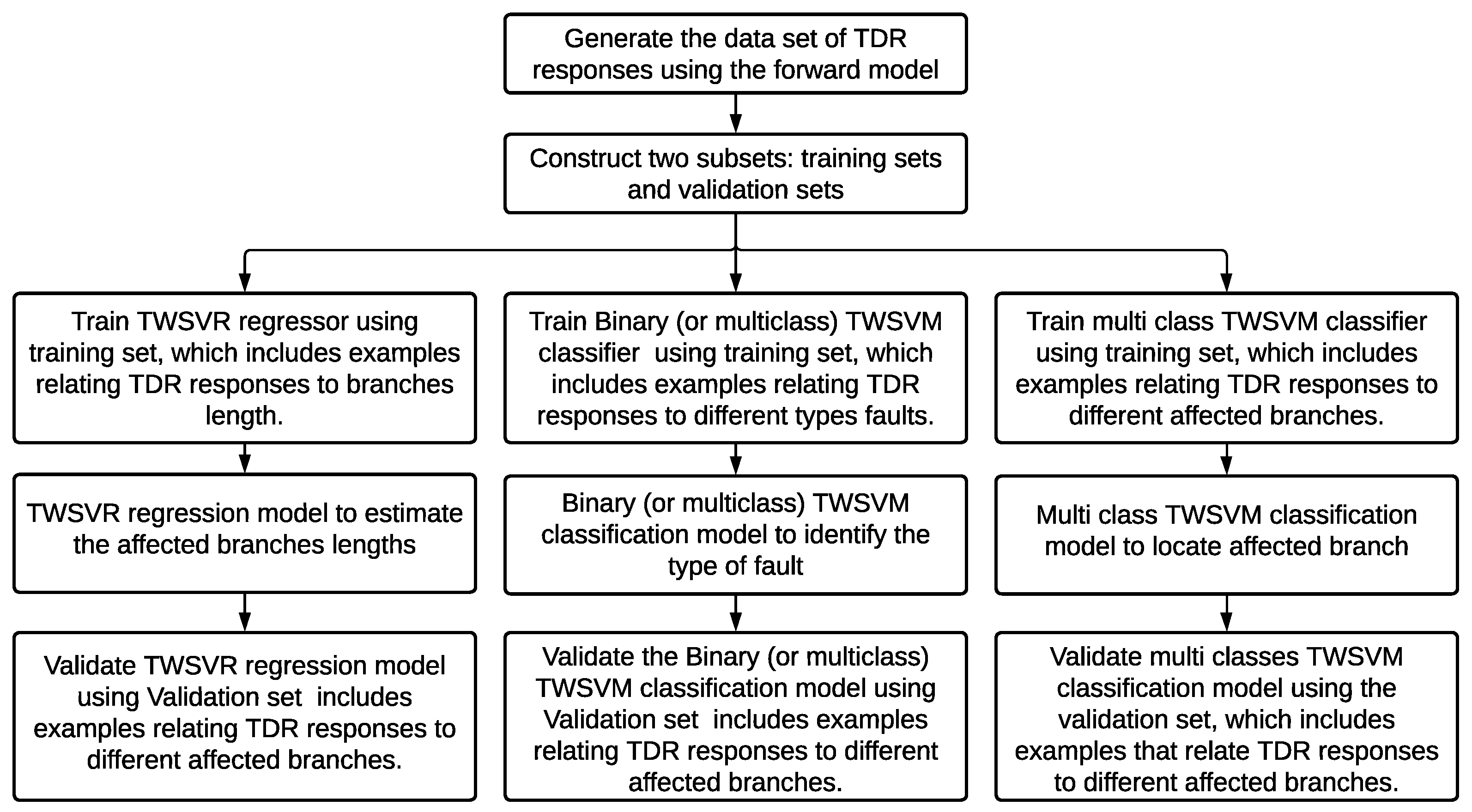
• A multiclass TWSVM classifier was formulated to determine the locations of affected branches. The dataset necessary for this multiclass TWSVM classification model comprises examples that relate TDR responses to various affected branches.
• Depending on the number of affected branches, a binary TWSVM classifier or multiclass TWSVM classifier is formulated to detect the type of fault:

  −

  In the case of the presence of only one fault in the wiring network under test, a binary TWSVM classier is sufficient to detect the type of the fault, which is either short circuit or open circuit

  −

  In the case of the presence of two or plus faults in the wiring network under test, a multiclass TWSVM classier is necessary to detect the type of the fault (short circuit faults, open circuit faults, or mix faults).

  The dataset necessary for this binary or multiclass TWSVM classification model comprises examples that relate TDR responses to the fault types.
• A TWSVR regressor is formulated to estimate the lengths of the affected branches. The dataset necessary for this TWSVR regressor model comprises examples that links TDR responses to branch lengths.

Figure 2. Flowchart of the offline process.

Figure 2. Flowchart of the offline process.

The online phase addresses the inverse problem by dividing it into three stages: detection, localization, and characterization. It is important to note that the design parameters for the localization and characterization stages vary based on the type of fault. In cases of soft faults within the wiring network, the fault impedance and location are considered design parameters. Conversely, for hard faults (open circuit or short circuit conditions), the design parameters include the lengths of branches and the loads on these branches. This study focuses solely on hard faults. The implementation of these three stages is illustrated in Figure 3 and further detailed subsequently.

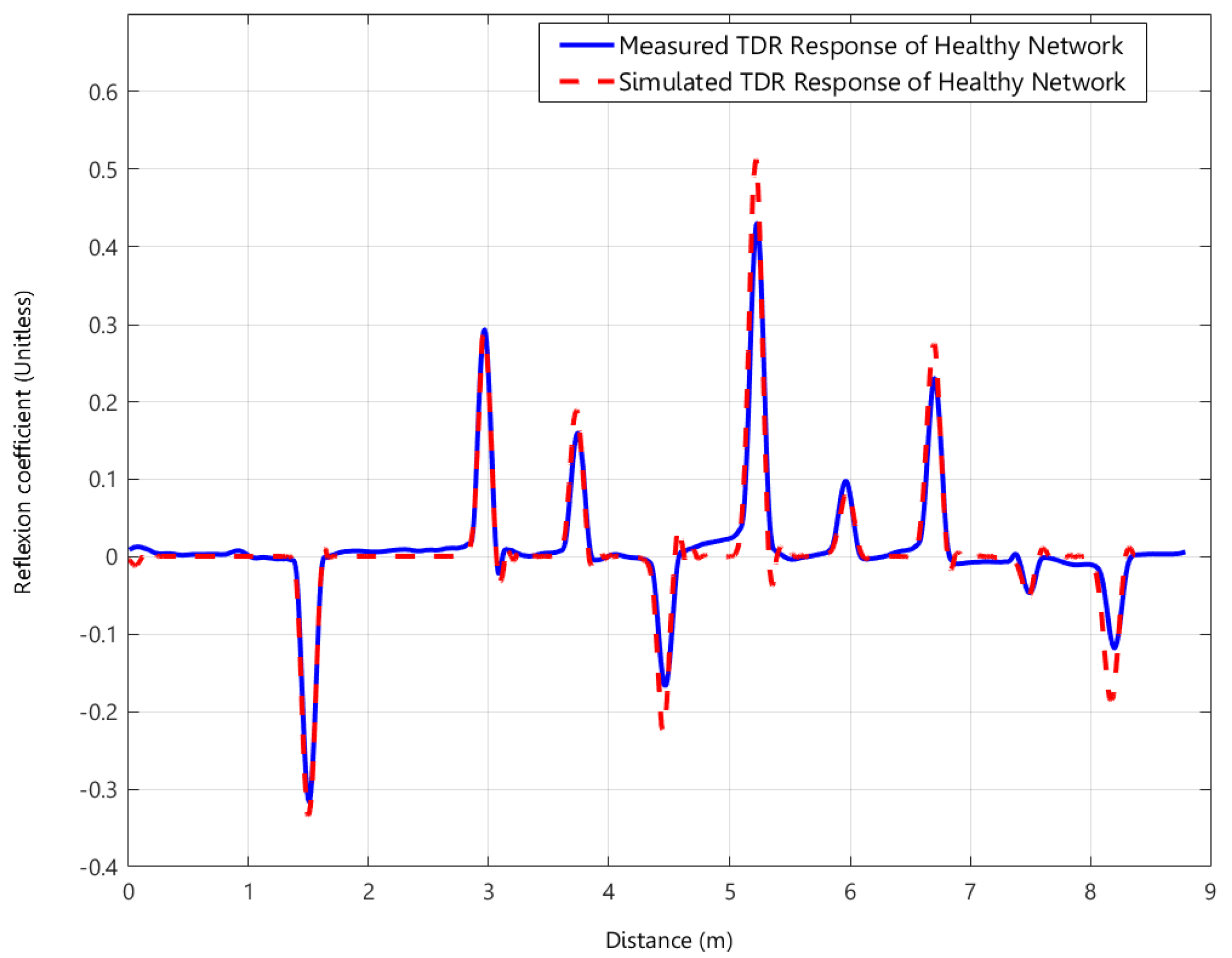
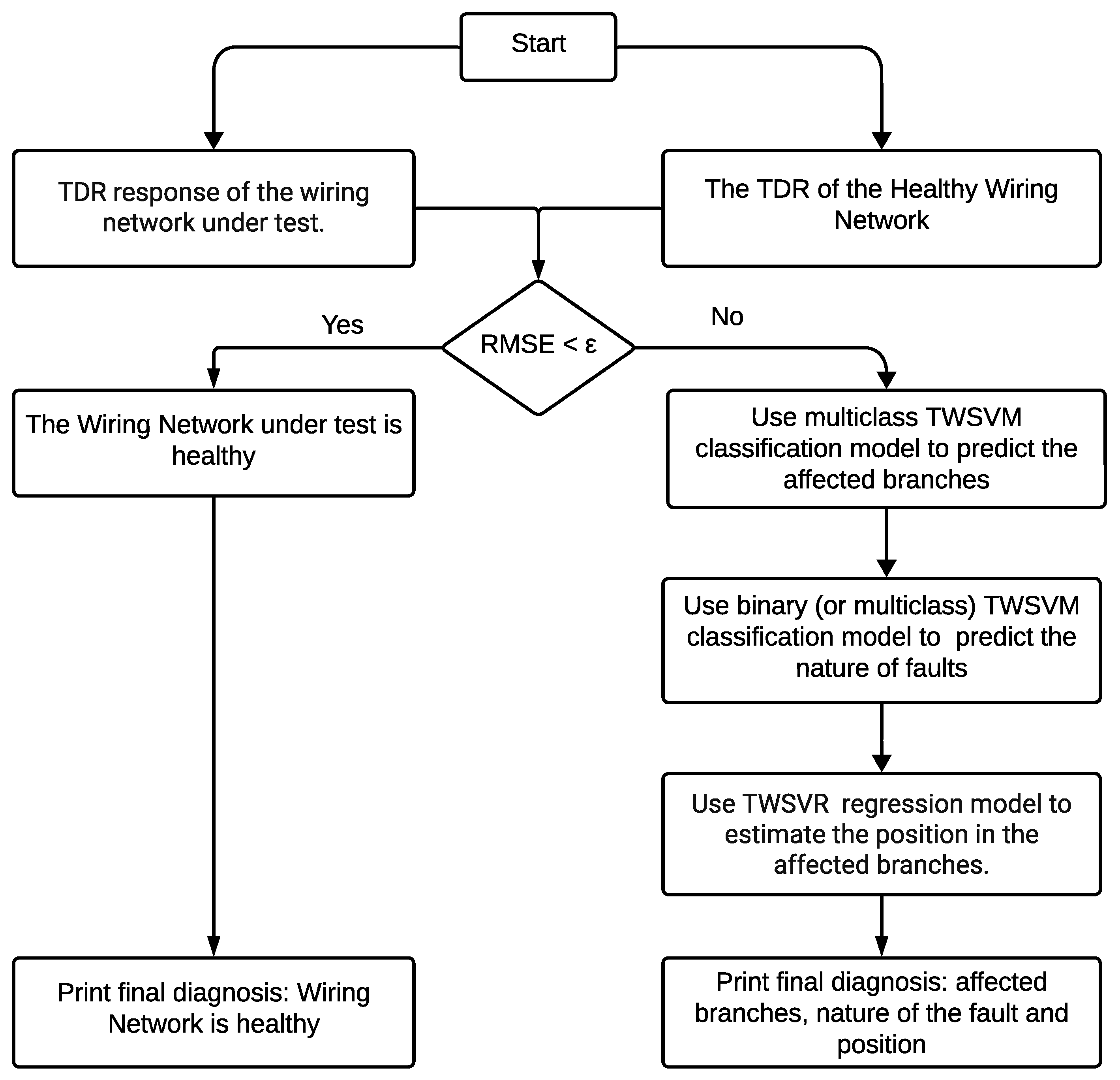
• In the detection stage, the TDR response from the WNUT, which is experimentally derived, is compared with a healthy network’s response (which is modeled forwardly). This comparison involve calculating the root mean square error (RMSE) between the WNUT’s response and that of a healthy network. If the RMSE falls below a predefined error threshold, the WNUT is deemed healthy; otherwise, it is considered compromised, prompting a progression to subsequent stages.
• The stages of localization and characterization involve (1) identifying the branches that are affected and ascertaining the type of faults and (2) estimating the lengths of these branches. The localization and characterization phases utilize the TWSVM classification and TWSVR models developed offline. Initially, the multiclass TWSVM classification model pinpoints the affected branches. Subsequently, the binary or multiclass TWSVM classification model determines the fault type. Lastly, the lengths of the impacted branches are estimated using the TWSVR model.

Remark 1. 

Depending on the complexity of the network, it is feasible to construct multiple classification and regression models. For a simple network, such as a Y-shaped network experiencing a single fault, it is sufficient to develop two classification models (alongside a single regression model to estimate the fault location within the affected branches): one to predict the affected branches and another to ascertain the fault type. In the case of a more complex network, such as a Y-Y-shaped network with two faults, it is advisable to partition the diagnostic challenge into various sub-problems and create classification and regression models for each. Both configurations, namely the Y-shaped network with a single fault and the Y-Y-shaped network with two faults, will be examined in the Numerical Results section.

5. Numerical Results

In this section, we explore three test configurations. The initial configuration comprises a Y-shaped wiring network with a single hard fault, while the second configuration also presents a Y-shaped network, this time with two hard faults located on distinct branches. The third configuration, more complex in nature, constitutes a YY-shaped wiring network in which two hard faults appear on separate branches. It should be noted that these configurations are already described in [16,17]. The objective of this paper is to reiterate these configurations as they represent common network configurations and to highlight the increased effectiveness of our proposed method in handling them.

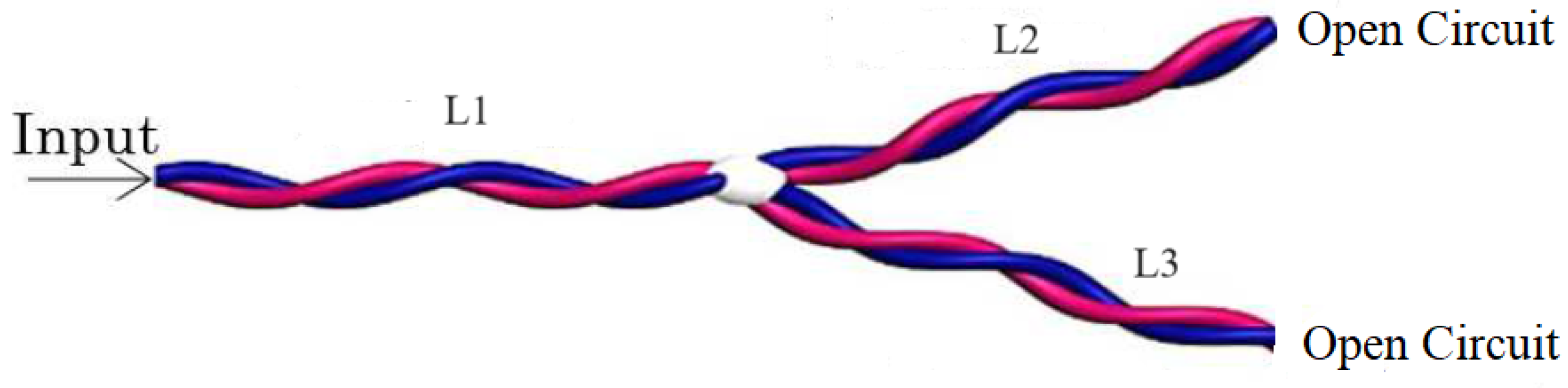
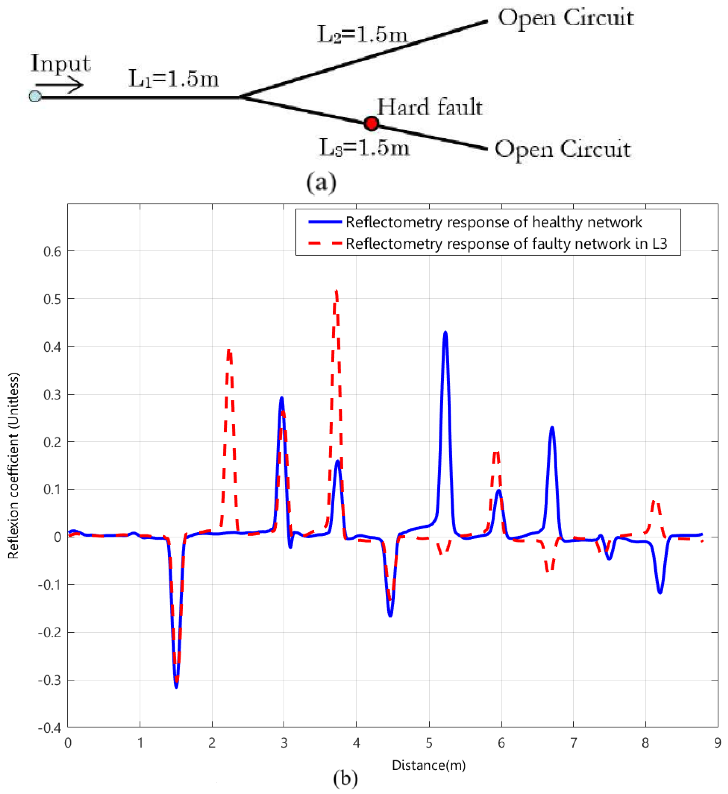
5.1. Diagnosis of a Y-Shaped Network Affected by One Hard Fault

The initial scenario under investigation involves a Y-shaped wiring network that consists of three wires with the following lengths: $L_1$ = 1.5 m, $L_2=1.5$ m, and $L_3=1.5$ m. The $L_2$ and $L_3$ branches were loaded with open circuits, as illustrated by Figure 4.

5.1.1. Offline Training and Evaluation of TWSVM for the Classification

The dataset for training the multiclass TWSVM classifier is generated using the forward model of the Y-shaped network configuration. This dataset comprises examples that associate TDR responses with the impacted branches. The specifics of the dataset employed for both training and validation of the multiclass TWSVM classifier include the following:

• Class 1: Indicates a hard fault on $L_1$, with 170 labeled responses.
• Class 2: Indicates a hard fault on $L_2$, with 60 labeled responses.
• Class 3: Indicates a hard fault on $L_3$, with 60 labeled responses.
• Class 4: Indicates a hard fault on $L_2$ and $L_3$, with 200 labeled responses.

The dataset was partitioned into training and testing subsets, with 80% assigned to training and 20% allocated for testing. Subsequently, a multiclass TWSVM classifier was developed using various kernel functions. This procedure was iterated 10 times, with the dataset randomly partitioned into training and testing subsets for each iteration. To assess the performance of the multiclass TWSVM classifier and identify the best kernel function, we employed metrics such as accuracy and macro average sensitivity.

$$\mathrm{Accuracy}\%={\displaystyle \frac{\mathrm{Number}\mathrm{of}\mathrm{Correct}\mathrm{Predictions}}{\mathrm{Total}\mathrm{Number}\mathrm{of}\mathrm{Predictions}}}\%$$

(10)

$$\mathrm{Macro}\mathrm{Average}\mathrm{Sensitivity}\%={\displaystyle \frac{1}{M}}\sum _{i=1}^M{\mathrm{Sensitivity}}_i\%,$$

(11)

where M represents the number of classes, and ${\mathrm{Sensitivity}}_i$ denotes the sensitivity for an individual class i, which is defined as follows:

$${\mathrm{Sensitivity}}_i\%={\displaystyle \frac{\mathrm{True}{\mathrm{Positives}}_{clas{s}_i}}{\mathrm{True}{\mathrm{Positives}}_{clas{s}_i}+\mathrm{False}{\mathrm{Negatives}}_{clas{s}_i}}}\%.$$

(12)

True Positives refer to labels correctly identified as belonging to class i, whereas False Negatives refer to labels incorrectly classified as belonging to class i when they do not.

Table 2. Accuracy and sensitivity as a function of kernel functions.

Kernel Functions	Accuracy %	Macro Average Sensitivity %
Linear	98.60 ± 0.035	97.33 ± 0.039
Polynomial	97.84 ± 0.051	96.25 ± 0.064
RBF	97.28 ± 0.062	95.03 ± 0.083
Sigmoid	95.92 ± 0.070	93.29 ± 0.131
Laplace	94.56 ± 0.121	91.12 ± 0.176

displays the accuracy and macro average sensitivity based on the kernel functions used. It was shown that the multiclass TWSVM classifier with the linear kernel function effectively differentiated between classes.

Remark 2. 

The TWSVM classifier, utilizing a linear kernel, has proven effective in resolving classification challenges related to the diagnosis of Y-shaped wiring networks. However, this efficacy may not be applicable to more complex wiring network configurations. Therefore, for more complex wiring network configurations, it is recommended to perform a new cross-validation with different kernels and to select the most suitable kernel based on the results obtained.

Remark 3. 

It is important to note that the class corresponding to a fault in $L_1$ and in the secondary $L_2$ or $L_3$ branches cannot be considered, as a hard fault in the main $L_1$ branch inhibits the propagation of the test signal to $L_2$ and $L_3$.

The proposed approach was comparatively assessed against the conventional SVM classifier by employing various kernels, random forest, and KNN classifiers. This study was conducted on an identical Y-shaped wiring network that was experiencing a hard fault in one branch. The dataset was once more partitioned into a training set and a validation set, with $80\%$ assigned for training and $20\%$ for validation. Subsequently, the multiclass TWSVM classifier with a linear kernel function, along with the multiclass SVM classifiers employing diverse kernel functions, random forest, and KNN classifiers, were trained. This process was iterated 10 times, with each iteration involving a random partitioning of the dataset into training and validation sets. To quantitatively evaluate the performance of the multiclass TWSVM classifier in comparison to other classifiers, the metrics of “accuracy and macro average sensitivity” were utilized. The outcomes are presented in

Table 3. TWSVM against conventional SVM, random forest, and k-nearest neighbor.

Methods	Accuracy (%)	Macro Average Sensitivity (%)
SVM-Laplacian	89.20%	85.34%
SVM-Linear	96.21%	93.20%
SVM-Polynomial	97.67%	96.17%
SVM-Sigmoid	56.38%	54.45%
SVM-RBF	94.85%	92.19%
TWSVM-Linear	98.60%	97.33%
Random Forest	97.56%	95.83%
K-Nearest Neighbor	91.84%	86.6%

. The table reveals that the multiclass TWSVM classifier with a linear kernel attained a notable accuracy of $98.60\%$ and a macro average sensitivity of $97.33\%$. The multiclass SVM classifier with a polynomial kernel ranked closely, achieving an accuracy of $97.66\%$ and a macro average sensitivity of $96.17\%$, followed by random forest. Other kernel types used with multiclass SVM classifiers and KNN classifiers demonstrated reduced competitiveness. Consequently, the TWSVM classifier with a linear kernel was validated as effective in addressing classification challenges in wiring network diagnostics for a Y-shaped network.

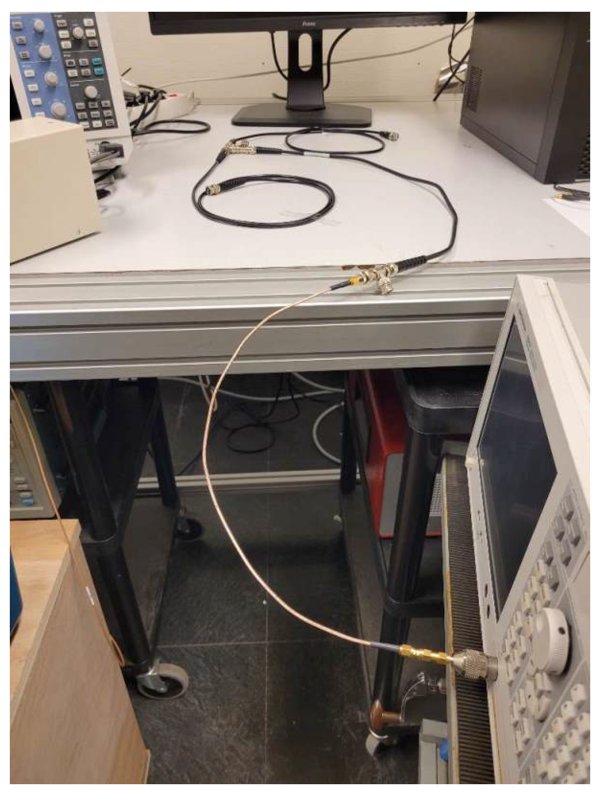
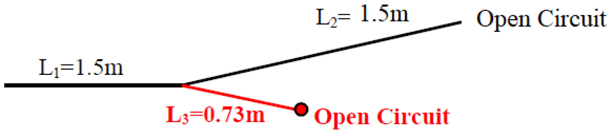
5.1.2. Online Diagnosis of the WNUT

Consider the Y-shaped wiring network, where a specific branch is impacted by a hard fault. The experimental setup, illustrated in Figure 5, involves the use of an Agilent Technologies (E5071C) Vector Network Analyzer (VNA) operating in the frequency domain, specifically ranging from 100 KHz to 4.5 GHz. Figure 6a shows a hard fault scenario in which an open circuit occurred in $L_3$. To illustrate the impact of this fault, Figure 6b presents a comparison between the experimentally obtained TDR response of the WNUT and the TDR response of the healthy network.

Initially, a comparison of the WNUT’s responses with those of a healthy reference was performed using the RMSE calculation. The RMSE value surpassed the set error threshold, suggesting faults in the WNUT. This led the algorithm to move into the phases of localization and characterization.

To pinpoint the defective branch, we utilized the multiclass TWSVM classifier model, which was developed and validated in the offline phase. This model can produce four output classes: Class 1 for a defect in $L_1$, Class 2 for a defect in $L_2$, Class 3 for a defect in $L_3$, and Class 4 for defects in both $L_2$ and $L_3$. The input for this classifier is the experimental TDR response from the WNUT, and it outputs the class of the affected branch. In this case, the classifier outputted Class 3, identifying $L_3$ as the defective branch. Following this identification, the binary TWSVM classifier model was used to ascertain the fault’s nature. The input was again the measured TDR response, and the output determined the fault type as either an open or a short circuit. For this instance, the classifier determined an ‘open circuit’ fault in $L_3$. After identifying the affected branch as $L_3$ and the fault as an open circuit, the next step was to estimate $L_3$’s new length using the TWSVR regressor model. Figure 7 illustrates the reconstructed network.

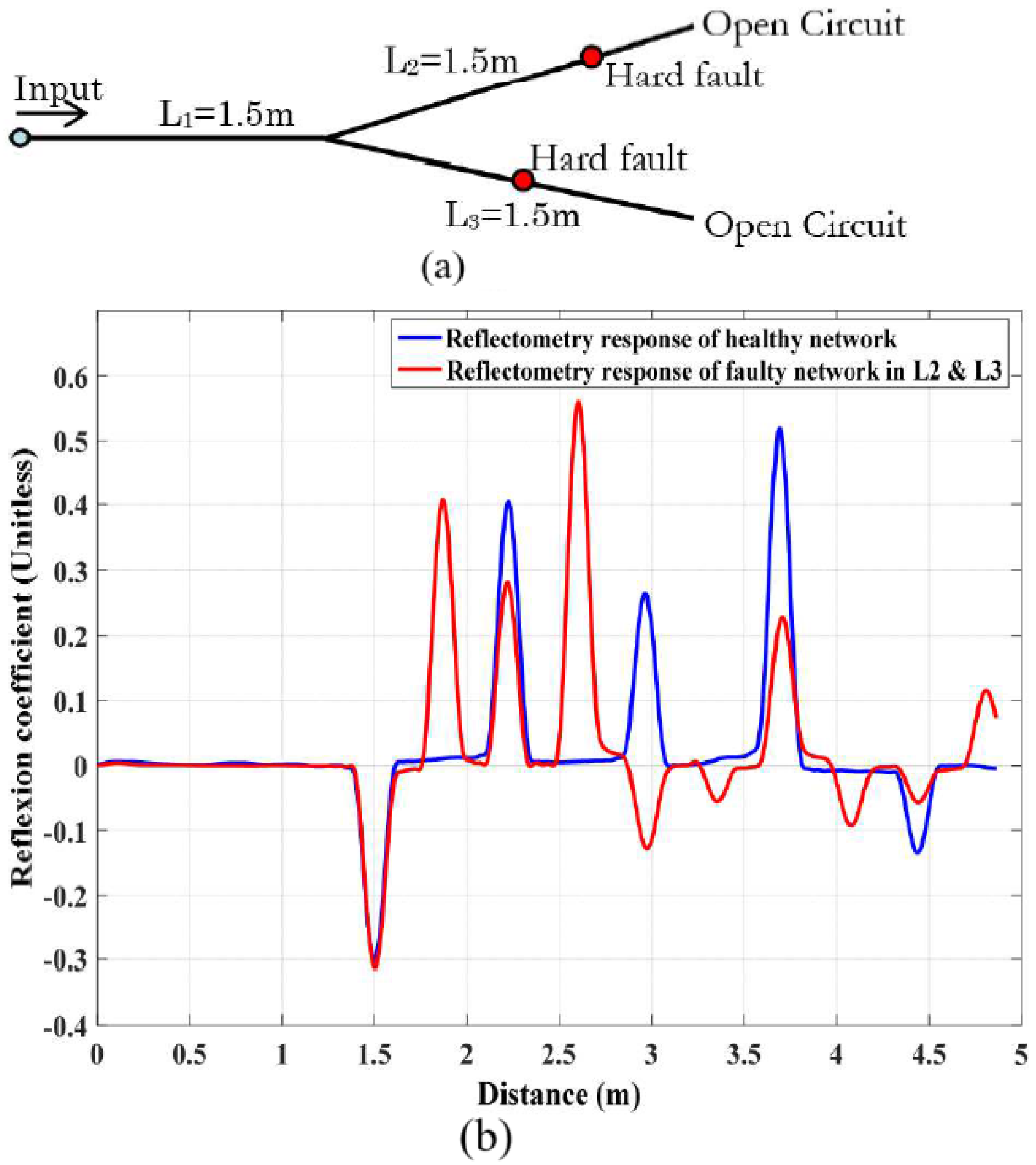
5.2. Diagnosis of the Y-Shaped Network Affected by Two Hard Faults

In this scenario, a Y-configured wiring network encountered two hard faults on distinct branches. This network comprises three wires, each measuring $L_1=1.5$ m, $L_2=1.5$ m, and $L_3=1.5$ m, where the $L_2$ and $L_3$ branches are loaded with open circuits. Figure 8a illustrates the situation where the two hard faults occur on $L_2$ and $L_3$. Figure 8b presents a comparison of the TDR responses for both healthy and faulty networks.

Similar to the first case studied, the calculation of the RMSE metric between the TDR response of the WNUT and the TDR response of the healthy network indicated that the wiring network was faulty.

To determine the affected branches of the wiring network due to the defect, we employed the multiclass TWSVM classifier model, which was developed and validated offline. It is important to note that this model can be classified into four categories: Class 1 for a hard fault on $L_1$, Class 2 for a hard fault on $L_2$, Class 3 for a hard fault on $L_3$, and Class 4 for a hard fault on both $L_2$ and $L_3$. In our case, the output from the multiclass TWSVM classifier model was Class 4, indicating that the $L_2$ and $L_3$ branches were compromised. After recognizing which branches were affected, we used the binary TWSVM classifier model to specifically identify the fault type. The binary TWSVM classifier model, which takes the measured TDR of the faulty network as input and outputs the fault type, indicated an open circuit hard fault in both $L_2$ and $L_3$. After determining the affected branches and the type of fault, the next step was to locate the fault. This was achieved using the TWSVR model, which outputted the new lengths for $L_2$ and $L_3$. The updated network configuration is illustrated in Figure 9.

Remark 4. 

In order to simplify and effectively demonstrate the workings of our approach, we made an assumption that when two hard faults occur, they are of an identical type. However, our method can be adapted to manage cases where two different types of faults occur by incorporating a multiclass TWSVM classifier rather than a binary TWSVM classifier to determine the types of faults.

5.3. Diagnosis of a YY-Shaped Network Affected by One or Two Hard Faults

Consider a YY-Shaped wiring network, where a pair of specific branches are affected by a hard fault. Figure 10 presents a scenario of hard faults, where an open circuit is evident in $L_2$ and $L_5$. To demonstrate the consequences of these faults, Figure 11 offers a comparative analysis between the experimentally obtained TDR response of the WNUT and the TDR response of the healthy network.

Given the intricate nature of the wiring network, we propose to perform the diagnostic process by decomposing the offline learning process into distinct sub-problems. This approach aims to facilitate the construction of various binary and multiclass TWSVM classification models, as well as TWSVR regression models.

• A first binary TWSVM classification model was created to identify the number of faults in the network (either one fault or two faults). To construct this model offline, the dataset was divided into two parts. One part includes the TDR responses that represent a single fault in the Y-Y network, while the other part consists of TDR responses that are affected by two faults.
• A second multiclass TWSVM classification model was created for the case of a single fault, following a similar approach to the model described in the Section 5.1 but with additional branches (we had $L_1$, $L_2$, $L_3$, $L_4$, and $L_5$ in this case). The construction of this model in an offline setting involves utilizing TDR responses that depict the occurrence of a single fault within the Y-Y network across various branches.
• A third binary TWSVM classification model was created for the case of a single fault in order to identify the nature of the fault (open or short).
• A fourth multiclass TWSVM classification model was created specifically for scenarios involving two faults. In order to construct this model offline, TDR responses representing the occurrence of two faults in various branches of the Y-Y network were utilized.
• A fifth multiclass TWSVM classification model was created for the case of two faults in order to identify the nature of the faults (i.e., whether both faults are open or both faults are short, as well as whether the first fault is a short circuit, the second an open circuit, or vice versa).
• Two TWSVR regression models were developed, one for the case of a single fault and another for the case of two faults, with the aim of estimating the lengths of the impacted branches.

Remark 5. 

It is crucial to emphasize that the scenarios depicting the occurrence of dual faults—one afflicting $L_1$ and the other found within the secondary branches of $L_2$, $L_3$, $L_4$, or $L_5$ are inherently unfeasible. This impossibility extends to cases where a fault is placed on $L_3$ simultaneously with another on the subsequent $L_4$ or $L_5$ branches. The rationale lies in the severe disruption that a hard fault imposes on the main $L_1$ branch, rendering it utterly impossible for the test signal to propagate through $L_2$, $L_3$, $L_4$, and $L_5$. Similarly, in the event where $L_3$ succumbs to a hard fault, the obstruction is such that it completely inhibits the test signal from reaching both $L_4$ and $L_5$.

Initially, the detection phase, which involves calculating the RMSE between the WNUT response and the healthy reference, indicated that the YY-wiring network was compromised. To ascertain the number of faults present, the first binary TWSVM classifier, which was developed and validated in an offline setting, was employed. This classifier revealed the existence of two hard faults. Subsequently, the second multiclass TWSVM classifier, also validated offline, was utilized to identify the affected branches. Its analysis revealed that the $L_2$ and $L_5$ branches were affected. Consequently, the fourth multiclass TWSVM classifier was employed to determine the nature of the faults. The results indicate that the $L_2$ and $L_5$ branches were afflicted with an open circuit hard fault. This validates the characterization step. Following the identification of the affected branches and the fault type, the final step entailed locating the fault positions using a TWSVM regression model, which was also validated offline. This model provided the new lengths for the $L_2$ and $L_5$ branches. The reconfigured network is depicted in Figure 12.

6. Conclusions

In this paper, we introduced a novel methodology for diagnosing wiring networks, which employs a combination of TDR responses and TWSVM. In the initial phase, the forward model, based on a numerical approach, was utilized to simulate the wiring network’s response under various fault conditions, thereby generating TDR responses. These TDR responses were then subsequently incorporated into the TWSVM models with kernel functions to accurately ascertain the condition of the network. The efficacy of this method was rigorously assessed, achieving a notable accuracy of 98.60% and a macro average sensitivity of 97.33%. This methodology presents several enhancements over conventional diagnostic techniques by improving computational speed and classification precision while preserving high diagnostic accuracy. By effectively addressing the complexity and nonlinearity of TDR responses, the proposed approach ensures optimized performance and the reliability of wiring network diagnoses. This comprehensive strategy not only augments system reliability and performance, but it also fosters the long-term sustainability of industrial systems by reducing environmental impact and improving operational efficiency.

References

1. Furse, C.; Chung, Y.; Lo, C.; Pendayala, P. A critical comparison of reflectometry methods for location of wiring faults. Smart Struct. Syst. 2006, 2, 25–46. [Google Scholar] [CrossRef]
2. Furse, C.; Haupt, R. Down to the wire: Aging, brittle wiring within aircraft poses a hidden hazard that emerging technologies aim to address. IEEE Spectr. 2001, 28, 34–39. [Google Scholar] [CrossRef]
3. Sharma, C.; Furse, C.; Harrison, R. Low-power STDR CMOS sensor for locating faults in aging aircraft wiring. IEEE Sens. J. 2006, 7, 43–50. [Google Scholar] [CrossRef]
4. Furse, C.; Smith, P.; Safavi, M.; Lo, C. Feasibility of spread spectrum sensors for location of arcs on live wires. IEEE Sens. J. 2005, 5, 1445–1450. [Google Scholar] [CrossRef]
5. Lelong, A.; Carrion, M. On line wire diagnosis using multicarrier time domain reflectometry for fault location. In Proceedings of the SENSORS, 2009, Canterbury, New Zealand, 25–28 October 2009; IEEE: Piscataway, NJ, USA, 2009; pp. 751–754. [Google Scholar]
6. Furse, C.; Chung, Y.C.; Dangol, R.; Nielsen, M.; Mabey, G.; Woodward, R. Frequency-domain reflectometry for on-board testing of aging aircraft wiring. IEEE Spectr. 2003, 45, 306–315. [Google Scholar]
7. Shi, Y.J. Theory and Application of Time-Frequency Analysis to Transient Phenomena in Electric Power and Other Physical Systems. Ph.D. Thesis, University of Texas, Austin, TX, USA, 2004. [Google Scholar]
8. Cheng, J.; Zhang, Y.; Yun, H.; Wang, L.; Taylor, N. A Study of Frequency Domain Reflectometry Technique for High-Voltage Rotating Machine Winding Condition Assessment. Machines 2023, 11, 883. [Google Scholar] [CrossRef]
9. Chilan, M.; Pirhadi, A.; Asadi, S.; Helfert, S. Analysis of multiconductor transmission lines using the time domain method of lines. AEU-Int. J. Electron. Commun. 2021, 138, 153863. [Google Scholar] [CrossRef]
10. Honarbakhsh, B.; Asadi, S. Analysis of multiconductor transmission lines using the CN-FDTD method. IEEE Trans. Electromagn. Compat. 2017, 1, 184–192. [Google Scholar] [CrossRef]
11. Paul, C.R. Analysis of Multiconductor Transmission Lines; John Wiley & Sons: Hoboken, NJ, USA, 2007. [Google Scholar]
12. Osman, O.; Sallem, S.; Sommervogel, L.; Carrion, M.; Bonnet, P.; Paladian, F. Distributed reflectometry for soft fault identification in wired networks using neural network and genetic algorithm. IEEE Sens. J. 2020, 20, 4850–4858. [Google Scholar] [CrossRef]
13. Zhang, L.; Zhao, Z.; Zhang, D.; Luo, C.; Li, C. Particle swarm optimization pattern recognition neural network for transmission lines faults classification. Intell. Data Anal. 2022, 26, 189–203. [Google Scholar] [CrossRef]
14. Chang, S.; Park, J. Wire mismatch detection using a convolutional neural network and fault localization based on time–frequency-domain reflectometry. IEEE Trans. Ind. Electron. 2018, 66, 2102–2110. [Google Scholar] [CrossRef]
15. Laib, A.; Terriche, Y.; Melit, M.; Su, C.L.; Mutarraf, M.; Bouchekara, H.; Guerrero, J.; Boudjefdjouf, H. Enhanced artificial intelligence technique for soft fault localization and identification in complex aircraft microgrids. Eng. Appl. Artif. Intell. 2024, 127, 107289. [Google Scholar] [CrossRef]
16. Smail, M.; Sellami, Y.; Bouchekara, H.; Boubezoul, A. Wiring Diagnosis using Time Domain Reflectometry and Random Forest. In Proceedings of the 2019 22nd International Conference on the Computation of Electromagnetic Fields (COMPUMAG), Paris, France, 15–19 July 2019; pp. 1–4. [Google Scholar]
17. Smail, M.; Boubezoul, A.; Bouchekara, H.; Sellami, Y. Wiring networks diagnosis using time-domain reflectometry and support vector machines. IET Sci. Meas. Technol. 2020, 14, 220–224. [Google Scholar] [CrossRef]
18. Banerjee, R.; Jamshed, A.; Haque, N. Localization of Faults in Coaxial Cables using Time-Domain Reflectometry and Support Vector Machine. In Proceedings of the 2023 IEEE 3rd Applied Signal Processing Conference (ASPCON), Haldia, India, 24–25 November 2023; pp. 242–245. [Google Scholar]
19. Laib, A.; Chelabi, M.; Terriche, Y.; Melit, M.; Boudjefdjouf, H.; Ahmed, H.; Chedjara, Z. Enhanced complex wire fault diagnosis via integration of time domain reflectometry and particle swarm optimization with least square support vector machine. IET Sci. Meas. Technol. 2024, 18, 417–428. [Google Scholar] [CrossRef]
20. Goudjil, A.; Smail, M.; Pichon, L.; Bouchekara, H.; Javaid, M. Wiring networks diagnosis using K-Nearest neighbour classifier and dynamic time warping. Nondestruct. Test. Eval. 2024, 39, 1–18. [Google Scholar] [CrossRef]
21. Jayadeva; Khemchandani, R.; Chandra, S. Twin support vector machines for pattern classification. IEEE Trans. Pattern Anal. Mach. Intell. 2007, 29, 905–910. [Google Scholar] [CrossRef] [PubMed]
22. Jayadeva; Khemchandani, R.; Chandra, S. Twin Support Vector Machines: Models, Extensions and Applications; Springer Publishing Company, Incorporated: Berlin/Heidelberg, Germany, 2018. [Google Scholar]
23. Tanveer, M.; Rajani, T.; Rastogi, R.; Shao, Y.H.; Ganaie, M. Comprehensive review on twin support vector machines. Ann. Oper. Res. 2024, 339, 1223–1268. [Google Scholar] [CrossRef]
24. Tanveer, M.; Tiwari, A.; Choudhary, R.; Jalan, S. Sparse pinball twin support vector machines. Appl. Soft Comput. 2019, 78, 164–175. [Google Scholar] [CrossRef]
25. Shao, Y.H.; Chen, W.J.; Zhang, J.J.; Wang, Z.; Deng, N.Y. An efficient weighted Lagrangian twin support vector machine for imbalanced data classification. Pattern Recognit. 2014, 47, 3158–3167. [Google Scholar] [CrossRef]
26. Wang, Z.; Shao, Y.H.; Wu, T.R. A GA-based model selection for smooth twin parametric-margin support vector machine. Pattern Recognit. 2013, 46, 2267–2277. [Google Scholar] [CrossRef]
27. Rastogi, R.; Sharma, S. Fast Laplacian twin support vector machine with active learning for pattern classification. Appl. Soft Comput. 2019, 74, 424–439. [Google Scholar] [CrossRef]
28. Tanveer, M.; Gautam, C.; Suganthan, P. Comprehensive evaluation of twin SVM based classifiers on UCI datasets. Appl. Soft Comput. 2019, 83, 105617. [Google Scholar] [CrossRef]
29. Xie, J.; Hone, K.; Xie, W.; Gao, X.; Shi, Y.; Liu, X. Extending twin support vector machine classifier for multi-category classification problems. Intell. Data Anal. 2013, 17, 649–664. [Google Scholar] [CrossRef]
30. Shao, Y.H.; Chen, W.J.; Huang, W.B.; Yang, Z.M.; Deng, N.Y. The best separating decision tree twin support vector machine for multi-class classification. Procedia Comput. Sci. 2013, 17, 1032–1038. [Google Scholar] [CrossRef]
31. Xu, Y. K-nearest neighbor-based weighted multi-class twin support vector machine. Neurocomputing 2016, 205, 430–438. [Google Scholar] [CrossRef]
32. Ding, S.; Zhao, X.; Zhang, J.; Zhang, X.; Xue, Y. A review on multi-class TWSVM. Artif. Intell. Rev. 2017, 52, 775–801. [Google Scholar] [CrossRef]
33. Jayadeva; Khemchandani, R.; Chandra, S. TWSVR: Twin support vector machine based regression. In Twin Support Vector Machines. Studies in Computational Intelligence; Springer: Cham, Switzerland, 2017; pp. 63–101. [Google Scholar]
Figure 1. Comparison of the simulation results and measurements for the TDR responses.
Sustainability 17 01836 g001
Figure 3. Flowchart of the online process.
Sustainability 17 01836 g003
Figure 4. Y-shaped wiring network.
Sustainability 17 01836 g004
Figure 5. The experimental setup.
Sustainability 17 01836 g005
Figure 6. (a) A Y-shaped network with a single hard fault, and (b) the TDR responses of the healthy network compared to the fault-affected network.
Sustainability 17 01836 g006
Figure 7. The reconstructed wiring network.
Sustainability 17 01836 g007
Figure 8. (a) A Y-shaped network with two hard faults, and (b) the TDR responses for the healthy and faulty networks.
Sustainability 17 01836 g008
Figure 9. The reconstructed wiring network.
Sustainability 17 01836 g009
Figure 10. A YY-shaped network exhibiting two hard faults (represented as open circuits).
Sustainability 17 01836 g010
Figure 11. The TDR response measurement of the faulty network in comparison to the TDR response of the healthy network.
Sustainability 17 01836 g011
Figure 12. The reconstructed YY-shaped network.
Sustainability 17 01836 g012