Article

Lagged and Instantaneous Effects Between Vegetation and Surface Water Storage in the Yellow River Basin

1
Collage of Geography and Environment, Shandong Normal University, Jinan 250358, China
2
Shandong Institute of Territorial and Spatial Planning, Jinan 250014, China
*
Author to whom correspondence should be addressed.
Sustainability 2025, 17(4), 1709; https://doi.org/10.3390/su17041709
Submission received: 9 January 2025 / Revised: 8 February 2025 / Accepted: 15 February 2025 / Published: 18 February 2025

Abstract

:
In recent years, large-scale afforestation in the Yellow River Basin (YRB) has attracted widespread attention due to its significant impact on surface water, playing a crucial role in the ecological sustainability and high-quality development of the basin. In this study, we used a combination of Theil–Sen and Mann–Kendall trend analysis to detect the spatiotemporal dynamic changes of NDVI, surface water storage (SWS), and its components in the YRB from 2001 to 2020, and explored the time lag and instantaneous effects between them using methods such as cross-correlation. The results show that from 2001 to 2020, NDVI and SWS in the YRB increased at rates of 0.41%/year and 1.95 mm/year, respectively, with fluctuations. Spatially, NDVI exhibited a significant upward trend in most areas of the YRB, while regions with significant increases in SWS, canopy surface water (CSW), snow water equivalent (SWE), and soil moisture (SM) were primarily located in the upper reaches. There was a time lag effect of about 2 months between NDVI and SWS in the YRB, and the time lags between SWE, SM, and NDVI were 5 months and 2 months, respectively. Except for CSW, the lag between NDVI and SWE was longer than that between NDVI and SWS or SM across all land cover types. Regarding the instantaneous effect, we found that the effect of vegetation on SWS in the upstream area is mainly the water storage function. In some areas of the middle and lower reaches, vegetation intensifies the consumption of SWS. Our study provides valuable insights into the response mechanism between vegetation restoration and SWS changes, facilitating better coordination between water resource management and ecological conservation in the YRB, thereby achieving sustainable regional economic and ecological development.

1. Introduction

Terrestrial water constitutes a crucial determinant and a pivotal factor influencing vegetation growth. Nearly half of the global vegetation growth is under the direct influence of water, profoundly shaping the worldwide carbon and oxygen balance [1,2]. Simultaneously, as an integral component of terrestrial ecosystems, vegetation assumes a substantial role in regulating and harmonizing both regional and global water resources [3]. Additionally, vegetation changes caused by natural environmental fluctuations and human activities have profound effects on surface water circulation and the ecological environment. Therefore, clarifying the dynamic changes of surface water and vegetation, as well as the impact of vegetation changes on surface water, is crucial for regulating regional water resource balance. This will help promote the coordination of water resource conservation and ecological protection, achieving sustainable economic and ecological development in the YRB.
Currently, research on the relationship between water and vegetation primarily focuses on two dimensions: precipitation and soil moisture (SM). Wu et al. delved into the global-scale relationship between vegetation and precipitation, revealing a discernible lag effect of P on vegetation changes [4]. Papagiannopoulou et al. expanded this exploration by investigating the response of vegetation to both precipitation and SM [5]. They found that water, as the predominant factor influencing vegetation growth, played a leading role in approximately 61% of global vegetation changes. While precipitation serves as a common indicator for studying terrestrial water, it offers only indirect observations of water. In arid regions with limited water resources, SM has proven effective in monitoring vegetation conditions [6,7]. Unlike precipitation, vegetation can directly utilize SM, obtaining moisture from the top layer of soil through remote sensing observations. However, the accuracy of estimating moisture at the roots of vegetation constrains the investigation of their relationship, impeding effective monitoring of vegetation root moisture status [8].
Moreover, alterations in vegetation also indirectly modify precipitation and SM conditions through changes in vegetation transpiration and terrestrial water circulation, consequently impacting terrestrial water dynamics [9,10]. Pertinent studies reveal that the augmentation of global surface vegetation contributes to 55% and 28% of the total evapotranspiration (ET) and precipitation, respectively [11]. At the watershed scale, vegetation changes exert significant effects on terrestrial water [12]. Feng et al. examined the impact of vegetation restoration on the Loess Plateau on watershed moisture and determined that vegetation transpiration exhibited a gradual increase with vegetation restoration, profoundly influencing regional hydrological conditions [13]. Changes in regional surface water, encompassing alterations in water storage within snow, vegetation canopy, soil, and other components, offer an effective means to estimate regional water shortages [14,15]. However, existing research on the impact of vegetation growth on land surface hydrology predominantly relies on single hydrological elements, lacking a comprehensive depiction of changes in regional surface water.
Presently, the Global Land Data Assimilation System (GLDAS), a terrestrial surface model system capable of providing real-time optimal land surface conditions at high resolution, is frequently employed for monitoring and assessing changes in surface water storage (SWS), drought, and SM content [16]. The GLDAS dataset offers global land surface data, encompassing precipitation, ET, SM content, and other hydrological elements. These data have undergone rigorous evaluation for suitability and enjoy widespread usage in China [17]. Consequently, the accuracy of SWS, calculated by extracting hydrological elements and employing the GLDAS land hydrological model, surpasses that of other products. Moreover, it exhibits superior spatiotemporal continuity compared to meteorological station observation data [18]. The normalized difference vegetation index (NDVI) proves to be a more accurate indicator of surface vegetation changes, offering a precise representation of vegetation dynamics [19]. Currently, medium- and long-term NDVI data primarily include AVHRR NDVI and MODIS NDVI. Among these, MODIS possesses higher spatial resolution than AVHRR, and the product quality of MODIS NDVI surpasses GIMMS NDVI. Consequently, MODIS NDVI finds extensive use in regional-scale and short- to medium-term time series research [20].
The Yellow River Basin (YRB) holds significance not only as a crucial economic and energy region but also as a vital ecological barrier in the country [21]. As one of China’s core food production areas, the region is rich in coal, natural gas, and hydroelectric resources. At the same time, the YRB plays a key role in wind and sand control, water conservation, and climate regulation, making it vital for the sustainable development of the region’s ecology and economy. The natural geographical environment of the YRB exhibits marked diversity, characterized by a fragile ecological environment, intricate habitats, and the pervasive occurrence of drought as a fundamental feature in the basin. The over-exploitation and utilization of water resources have led to water scarcity emerging as the most pressing issue in ecological environment management within the YRB [22]. In recent years, extensive implementation of vegetation restoration projects in the YRB has, to some extent, improved the regional ecological environment. However, this endeavor has also brought about profound changes in the spatial distribution and availability of water resources across the basin. Moreover, against the backdrop of escalating global warming, particularly the increasingly pronounced trend of warming and humidification in the northwest, there exists a substantial impact on the dynamic changes of water resources and vegetation within the YRB.
Currently, most studies focus on the dynamic monitoring of NDVI at the basin scale in the YRB and its relationship with climate and SM [19]. However, research on the relationship between vegetation and SWS is relatively scarce and cannot systematically reveal the connection between vegetation and SWS. This study, based on GLDAS SWS and MODIS NDVI data, addresses the following issues: 1) The spatiotemporal variation trend of vegetation and the components of surface SWS; and 2) the lag and instantaneous effects between vegetation and the components of SWS. The research findings reveal the relationship between vegetation and SWS in the YRB, which is helpful for better coordinating water resource management and ecological protection in the region, thus achieving sustainable economic and ecological development.

2. Materials and Methods
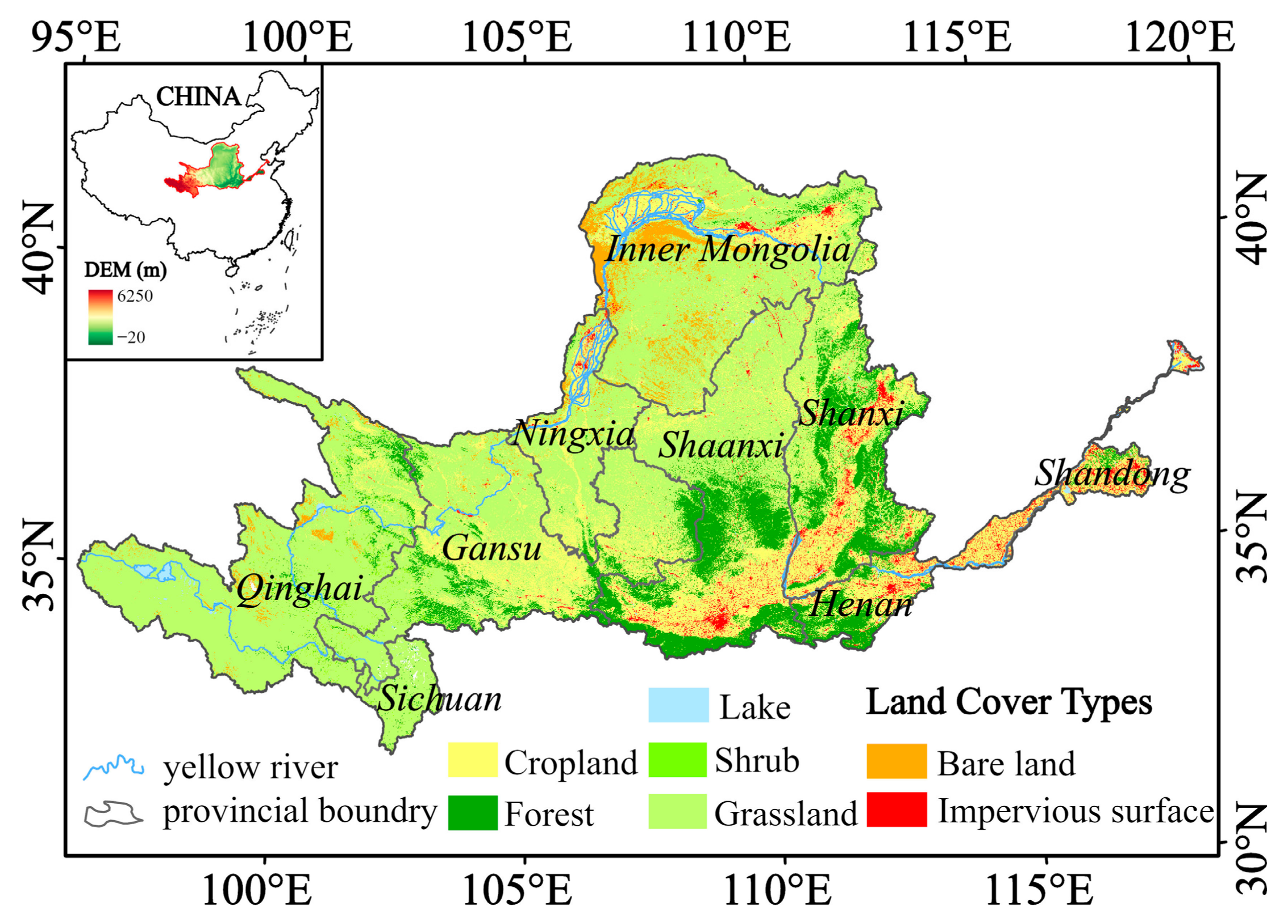
2.1. Study Area

The YRB (96°~119° E, 32°~42° N) is situated in northern China, covering an approximate area of 795,000 km2 [23]. The basin’s terrain forms a ladder shape from west to east. The precipitation and ET capacity in the YRB are influenced by ocean circulation and monsoon climate, displaying evident spatial variations and seasonal characteristics. Climate types within the basin predominantly include temperate monsoon, temperate continental, and plateau mountain climates. The primary vegetation cover types in the basin comprise forests, grasslands, shrubs, and farmland (Figure 1).

2.2. Data

The SWS data utilized in this study were sourced from the GLDAS, available at (https://disc.gsfc.nasa.gov/datasets?page=1&keywords=GLDAS (accessed on 2 February 2024). The GLDAS system is grounded in global terrestrial surface assimilation data derived from satellites, terrestrial surface models, and ground observation data [24]. It incorporates four terrestrial surface models, that is, Noah, VIC, CLM, and Mosaic. These models offer comprehensive data on temperature, ET, SM, snow water equivalent (SWE), canopy surface water (CSW), and other variables spanning from 1979 to the present. GLDAS provides two spatial resolutions (0.25° and 1°) and three temporal resolutions (3 h, daily, and monthly).
For this paper, the Noah model within the GLDAS assimilation data model (Table 1) is employed, encompassing 0~200 cm SM, SWE, and CSW, with subsequent computation of SWS data. The original Noah model data possess a spatial resolution of 0.25° and a temporal resolution of 1 month. In this study, the mean method is applied to derive interannual and seasonal data for SWS.
NDVI serves as a remote sensing indicator, reflecting vegetation activity and productivity [25]. It effectively expresses the status and characteristics of surface vegetation coverage. In this study, the data product MOD13Q1, supplied by NASA and available at https://disc.gsfc.nasa.gov, is utilized. This product features a spatial resolution of 250 m and a temporal resolution of 16 days. The maximum value composite method (MVC) is applied in this paper to derive monthly and annual NDVI data.
The land cover data utilized in this article were sourced from the inaugural Landsat-based China Land Cover Annual Dataset (CLCD), created by Yang et al. This dataset provides 30 m of annual land cover information and dynamic changes in China spanning from 1990 to 2022. It exhibits strong consistency with global forest change, global surface water, and three impervious surface products, underscoring its potential application value in global change research [26]. In alignment with the specific characteristics of the study area, this paper categorizes land cover types into the following six classes: farmland, forest, shrub, grassland, bare land, and impervious surface. The dataset is freely accessible at https://doi.org/10.5281/zenodo.4417810 (accessed on 14 September 2024).

2.3. Methodology

2.3.1. Calculation of SWS Based on GLDAS

Changes in regional surface water storage, including SWE, CSW, SM, and other elements, are important information for assessing regional SWS conditions [15,16]. Existing research suggests that vegetation growth in the YRB is directly related to CSW, SWE, and SM [27]. Therefore, this paper sums CSW, SWE, and SM to obtain the SWS value. The specific calculation formula is as follows:
S W S = S M + S W E + C S W
S M = S M 1 + S M 2 + S M 3 + S M 4
where SM1 represents SM content in the 0~10 cm depth interval, SM2 represents SM content in the 10~40 cm depth interval, SM3 represents SM content in the 40~100 cm depth interval, and SM4 represents SM content in the 100~200 cm depth interval.

2.3.2. Trend Analysis of Vegetation NDVI and SWS

To quantify the changing trends of SWS and vegetation in the YRB from 2001 to 2020, this paper employs a method that combines Theil–Sen median and Mann–Kendall. This approach facilitates the estimation and verification of trends in both SWS and vegetation NDVI in the YRB.
The Theil–Sen median trend analysis is employed for the estimation of slopes in long time series data [28]. The magnitude of the time series change trend is assessed by estimating the linear rate of change through the slope and intercept [29]. The calculation is as follows:
S V = m e d i a n V j V i j i , 2001 i < j 2020
where V represents the time series of a specific pixel. When SV > 0, it indicates an upward trend in the variable SV, otherwise it signifies a downward trend. The absolute value of SV provides an indication of the speed of change.
However, the Theil–Sen median trend analysis alone cannot ascertain the significance of time series trends [30]. Therefore, this paper employs the Mann–Kendall trend test for significance testing. This method is well-suited for the long-term trend analysis of variables, including hydrology, meteorology, and vegetation [2,31].
In this method, it is assumed that H0 (x1, x2, …, xn) is a sample set composed of n independent and identically distributed random variables, where Z represents the time series change, and its formula is as follows:
Z = S 1 V a r S > S > 0                   0               S = 0   S + 1 V a r S   S < 0
where
s = i = 1 n 1 j = i + 1 n s g n x j x i
V a r S = n n 1 2 n + 5 18
and
s g n x j x i = 1               x j x i > 0 0               x j x i = 0 1       x j x i < 0
In Equations (5) and (6), xi and xj refer to the sample time series datasets; n denotes the length of time, sgn represents the symbolic function; Z > 0 indicates an upward trend in the time series, Z < 0 indicates a downward trend, and Z = 0 denotes no change.

2.3.3. Time-Lag and Correlation Analysis Between Vegetation NDVI and SWS

This article employs lagged cross-correlation analysis with NDVI data and data on SWS and its components to calculate the maximum correlation coefficient between vegetation NDVI and SWS and its components, as well as the lag time between them in the YRB. The formula for lagged cross-correlation is as follows:
r k x , y = i = 1 n k x i x ¯ i y i + k y ¯ i + k i = 1 n k x i x ¯ i i = 1 n k y i + k y ¯ i + k
where   r k ( x , y ) represents the correlation coefficient series between NDVI and SWS and its components at lag time; k, x i , y i   are the correlation coefficient series between SWS and its components and NDVI; n is the length of the time series; and k is the time lag.
This paper employs Pearson’s correlation analysis to examine the spatiotemporal correlation between SWS and vegetation NDVI in the YRB. Additionally, the time lag of SWS on vegetation NDVI is quantified. The correlation analysis formula is calculated as follows:
R x y = i = 1 n x i x ¯ y i y ¯ i = 1 n x i x ¯ 2 i = 1 n y i y ¯ 2
where n refers to the total sample size; xi and yi represent the values of the variables x and y in the i-th year; and x ¯ and y ¯   denote the means of the two variables.

3. Results

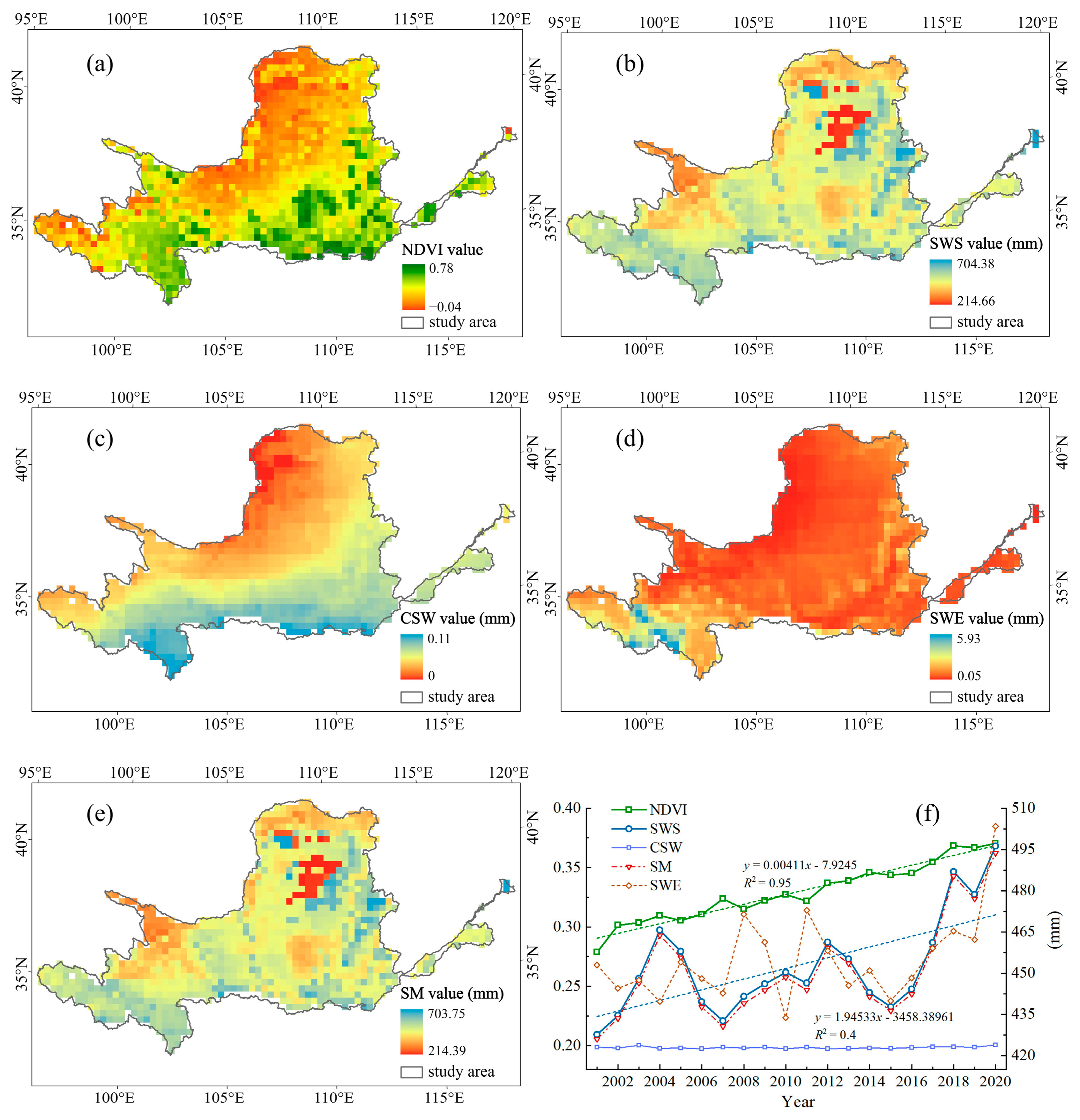
3.1. The Spatiotemporal Distribution Patterns of Vegetation NDVI, SWS, and Its Components

We, respectively, take the averaged values of vegetation NDVI, SWS, and its components accumulated from 2001 to 2020 in the YRB as the values of each factor for the 20-year study area, and obtain the spatiotemporal distribution patterns of NDVI, SWS, and its components (Figure 2) [32]. This study found that the NDVI and SWS in the YRB exhibit significant spatial heterogeneity. Overall, both NDVI and SWS show a decreasing distribution from southeast to northwest, and the reasons for this difference may be related to differences in climatic factors causing variations in water-thermal conditions and natural geographical environments. Specifically, the low NDVI values are mainly distributed in the northwest, while the areas with scarce SWS are distributed in the inland areas of the middle reaches of the Yellow River (MYR), among other places. In addition, regarding the spatial distribution of SWS components, CSW, SWE, and SM exhibit distinct spatial differences, each with its own characteristics. CSW shows a similar distribution pattern to vegetation NDVI, with a high-to-low distribution pattern from southeast to northwest. The high-value areas of SWE are concentrated in the river source area of the upper reaches of the Yellow River (UYR), while the remaining areas exhibit scarcity. It is noteworthy that the spatial distribution of SM is quite similar to that of SWS, and we found that SM is the main component of SWS in the YRB, which may be related to the loess soil in the basin. The loose structure of loess soil leads to severe infiltration of vegetation canopies and snowmelt, making SM content the main component of surface water.
This study also found that from 2001 to 2020, the overall trends of NDVI and SWS in the YRB exhibited fluctuating upward trends, with growth rates of approximately 0.41% per year and 1.95 mm per year, respectively. The fluctuation amplitude of SWS was much greater than that of NDVI, and SWS showed three distinct upward phases (2001–2004, 2007–2012, and 2015–2020) and two distinct downward phases (2004–2007 and 2012–2015). In addition, it was observed that CSW showed relatively stable overall changes over the 20 years, and it remained lower than other surface water components. The trend of SM changes was highly similar to that of SWS, indicating that SM in the YRB changes in accordance with SWS variations. Compared to CSW and SM, the fluctuation amplitude of SWE change was the most pronounced, which may be related to climate change and precipitation variability in the YRB. In summary, from 2001 to 2020, vegetation cover in the YRB significantly improved, while surface water, although fluctuating greatly, showed slight overall improvement; this change is significantly associated with SM.

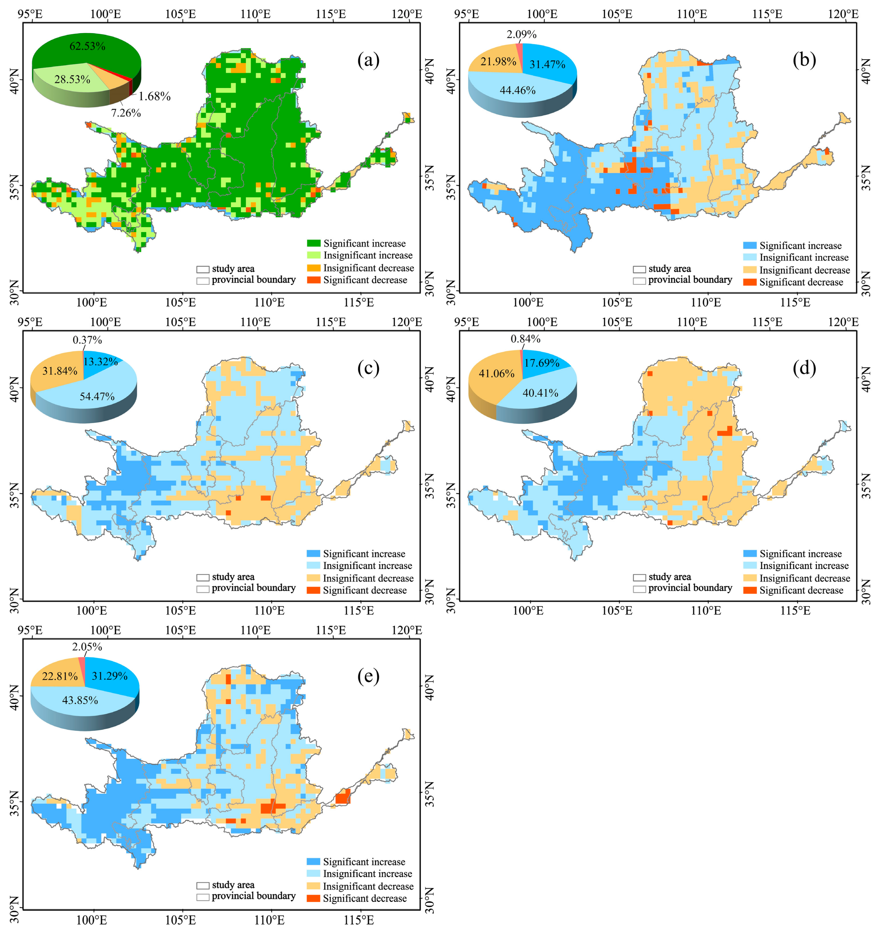
3.2. The Change Trends of Vegetation NDVI, SWS, and Its Components

At the pixel scale, we conducted trend analysis on the interannual changes of NDVI and SWS, along with its components, in the YRB from 2001 to 2020. This analysis allowed us to obtain the spatial distribution of the changing trends of each factor within the study area. Based on a 90% confidence level, we classified the significance of the results into four levels to obtain the spatial distribution of the significance of SWS change trends (Figure 3).
This study found that the trends and significance distributions of NDVI and SWS in the YRB from 2001 to 2020 exhibited significant spatial heterogeneity. In particular, the vegetation NDVI in the MYR and UYR showed a significant increasing trend, covering an area of 62.53%, while the areas with non-significant changes accounted for 35.79%; only 1.68% of sporadic regions exhibited a significant decreasing trend. Thus, overall, there was a significant increasing trend in vegetation NDVI in the YRB, indicating a gradual improvement in vegetation cover over the 20-year period. Regarding SWS, we found that in 31.47% of the YRB, surface water resources showed an increasing trend, mainly distributed in the UYR in Gansu and Qinghai provinces. Additionally, 66.44% of the area showed no significant change in SWS, mainly distributed in the MYR and LYR. This suggests that although there is no significant change in surface water resources in the MYR and lower reaches of the Yellow River (LYR), there appears to be a decreasing trend in the downstream areas.
In addition, we also investigated the changes in CSW, SWE, and SM in the YRB separately. This study found that there were significant spatial differences in the trends of CSW, SWE, and SM during the period from 2001 to 2020, and these spatial differences exhibited certain similarities. In terms of trend changes, the areas where CSW, SWE, and SM significantly increased are mainly distributed in the UYR, accounting for 13.32%, 17.69%, and 31.29% of the total area, respectively, while the MYR and LYR showed non-significant trend changes. Furthermore, we found that compared to CSW and SWE, the spatial distribution characteristics of SM trend changes are most similar to those of SWS, showing mainly increasing trends in the UYR, while some areas in the MYR and LYR exhibited decreasing trends. From the above results, it can be inferred that in most areas of the UYR from 2001 to 2020, surface water resources and their components showed a significant increasing trend, with SM exhibiting the most pronounced increase compared to CSW and SWE. Therefore, we attribute the main driving force behind the increase in surface water resources in the UYR to the increase in SM. Additionally, in the MYR and LYR, especially in the downstream areas, a decreasing trend was observed, highlighting the increasingly prominent issue of water scarcity.
In combination with land cover data, we also explored the trends of NDVI, SWS, CSW, SWE, and SM for different land cover types (Table 2). Among all land cover types, NDVI exhibited increasing trends, with the strongest and weakest positive trends observed in forests (0.039 century−1) and shrubs (0.021 century−1), respectively. Except for impervious surfaces, all land cover types showed increasing trends in SWS and its components (CSW, SWE, and SM). Compared to other land cover types, shrubs exhibited the strongest increasing trends in SWS and its components, with growth rates of 3.3 mm Year−1, 2.12 mm Year−1, 1.85 mm Year−1, and 3.29 mm Year−1, respectively. This indicates that shrubs play a more significant role in surface water retention. In other words, planting shrubs seems to be more beneficial for improving the regional surface water resources.

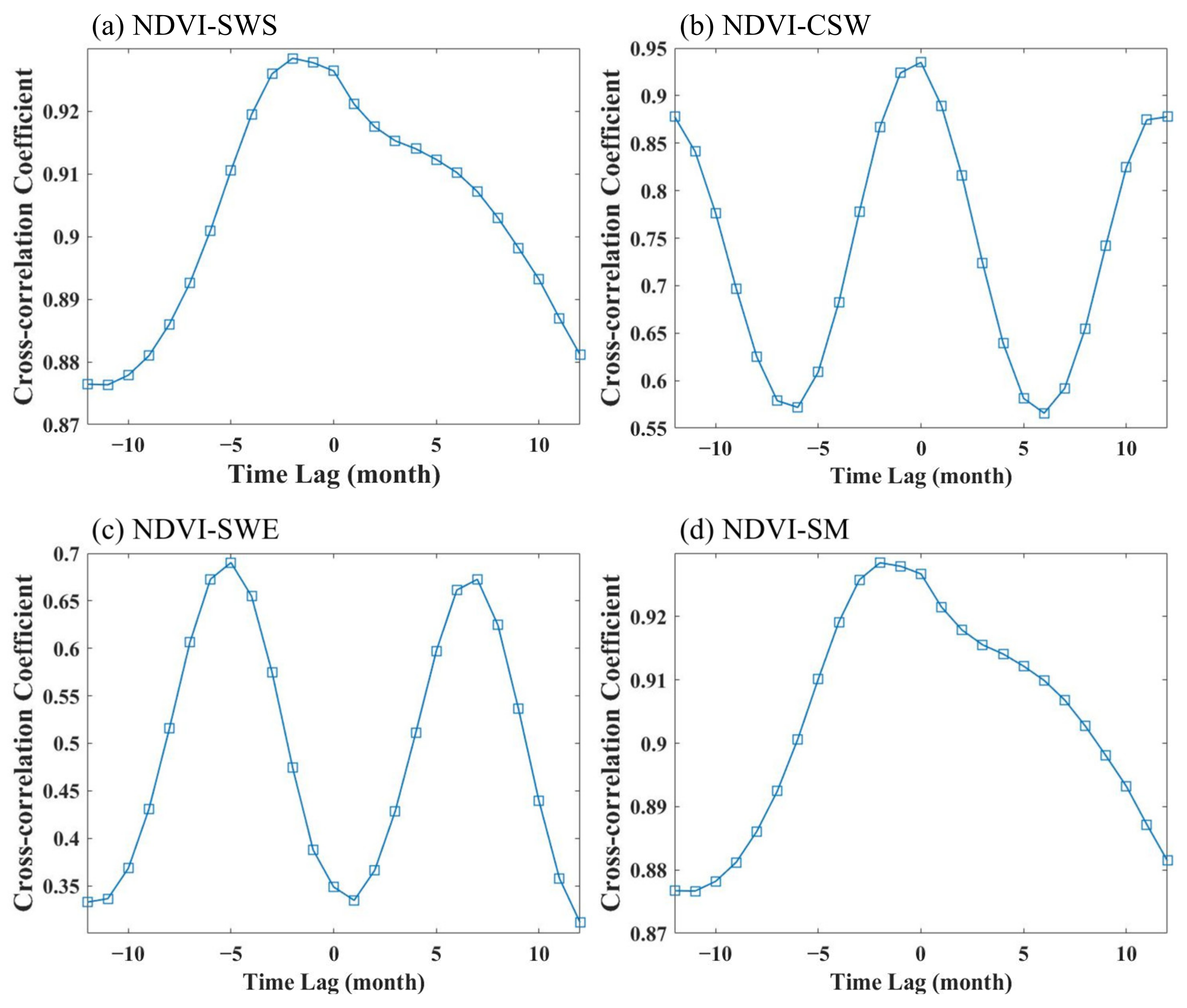
3.3. The Time Lag Effect of NDVI, SWS, and Its Components

To investigate the lag effect between vegetation and water, we conducted lag correlation analysis on the NDVI of vegetation and the components of SWS (CSW, SWE, and SM) in the YRB for lags ranging from 1 to 12 months, obtaining the maximum correlation coefficients at different lag times (Figure 4). The results indicate significant variations in the lag correlation between NDVI and SWS and its components in the YRB. Regarding the lag correlation between NDVI and SWS, we found that when the lag time T_SWE = 2, the correlation coefficient between NDVI and SWS was at its maximum. This suggests that SWS lags behind vegetation NDVI by approximately 2 months. With the extension of lag time, the lag correlation between NDVI and SWS gradually weakened, which may be related to the absorption of water by vegetation during the growth cycle.
Additionally, we observed different characteristics in the lagged correlations between vegetation NDVI and CSW, SWE, and SM. Specifically, when the lag times were T_CSW = 0, T_SWE = −5, and T_SM = −2, the lagged correlation between NDVI and CSW, SWE, and SM reached their maximum, respectively. This suggests that the lagged correlation between NDVI and CSW is not particularly significant. However, SWE lags behind vegetation NDVI by 5 months, while SM lags by 2 months. This lag difference may be related to the infiltration process of surface snow water and the availability of SM to vegetation roots. Furthermore, through comparison, we found that the lagged correlation between NDVI and SWS is highly similar to that with SM, not only in terms of the range of maximum correlation coefficients but also in the variation of lagged correlation. This indicates that the lagged correlation between NDVI and SWS is primarily associated with SM content.
The lagged correlations between NDVI and SWS, as well as its components, exhibit significant differences across different land cover types (Table 3). We found that, in terms of lag time, the lagged relationships between NDVI and SWS, as well as SM, are remarkably similar across different land cover types. This further confirms the assertion that the lagged correlation between NDVI and SWS in the YRB is primarily related to soil moisture content. Additionally, among all land cover types, the lagged relationship between NDVI and SM is shorter than that between NDVI and SWE, which is also associated with surface water infiltration and the availability of vegetation root zone moisture. In terms of the lagged relationship between NDVI and SWS, as well as SM, the lag times across different land cover types are as follows: forest (−3) = shrubland (−3) > farmland (−2) = impervious surface (−2) > grassland (−1) > bare land (0). This can be explained by the different structural characteristics among vegetation types.

3.4. The Instantaneous Effects of NDVI and SWS and its Components

The spatial correlation between NDVI and SWS along with its components is illustrated in Figure 5a. This study reveals significant spatial variations in the correlation between NDVI and SWS, with correlation coefficients between SWS and NDVI ranging from −0.65 to 0.94. Among these, approximately 84.08% of the area shows a positive correlation between SWS and vegetation NDVI, primarily distributed in the MYR and UYR. Approximately 15.92% of the area exhibits a negative correlation, mainly concentrated in the MYR and LYR, especially in the southern parts of Shaanxi, Shanxi, Ningxia, and some areas of Inner Mongolia. Furthermore, through a significant T-test for the correlation between NDVI and SWS, it is observed that the area passing the significance test accounts for approximately 36.87% of the total study area. Within this, 36.13% of the area demonstrates a significant positive correlation, mainly concentrated in Qinghai, Gansu, and the southern part of Ningxia in the UYR, as well as the northeastern part of Inner Mongolia.
Figure 5b–d, respectively, depict the spatial distribution of the correlation between NDVI and CSW, SWE, and SM. Overall, the spatial patterns of correlation between NDVI and CSW, SWE, and SM exhibit similarities, with the highest correlations appearing in areas such as Gansu and Qinghai in the UYR, while weak or even negative correlations are observed in the MYR and LYR. The proportions of positive correlation areas between NDVI and CSW, SWE, and SM are 67.6%, 60.8%, and 84.17%, respectively, among which the proportions passing significance tests are 15.74%, 11.92%, and 36.22%, respectively. Furthermore, it is observed that the correlation coefficients and significance levels between NDVI and SM, as well as SWS, not only exhibit similar spatial distributions but also have the closest range of correlation coefficients. It is noteworthy that in Qinghai in the UYR, there are significant differences in the correlation between NDVI and SWS and its components. Unlike CSW and SM, the correlation between NDVI and SWE shows a significant negative correlation, which may be related to regional snowmelt due to global warming.
To explore the differences in the correlation between NDVI and SWS and its components across various land cover types, we conducted a statistical analysis based on land cover data (Figure 6). We found that, except for bare land, the proportion of positive correlations between NDVI and SWS and its components is higher than that of negative correlations across other land cover types. Specifically, the maximum correlation coefficients between NDVI and SWS occur in forests (0.94), grasslands (0.92), farmland (0.89), bare land (0.8), impervious surfaces (0.7), and shrubs (0.64), respectively. Additionally, through comparison, we observed significant differences in the sensitivity of different land cover types to surface water. Among them, approximately 53.2% of grassland areas exhibit a positive correlation with surface water, while only 6% show a negative correlation. Therefore, compared to other land cover types, grasslands demonstrate the highest sensitivity, followed by farmland, forests, bare land, impervious surfaces, and shrubs. It is noteworthy that among the limited shrub vegetation in the YRB, its correlation with SWS and its components (CSW, SWE, and SM) is positive. This suggests that planting shrubs appears to be the most effective approach for improving regional surface water conditions during the vegetation restoration process.

4. Discussion

4.1. Drivers of Vegetation Changes and SWS

The variation trend of SWS in the YRB exhibits significant spatial heterogeneity (Figure 3b). Specifically, the SWS in the UYR shows a noticeable increasing trend throughout the study period, which may be associated with increased precipitation, glaciers, and snowmelt resulting from recent warming and humidification in the northwest region [33]. On the one hand, with regional climate warming and increased humidity, variables associated with snowfall in the UYR show a decreasing trend, leading to an increase in the total runoff in the Yellow River source area [34]. On the other hand, it may also be related to the increase in precipitation in the UYR, leading to the melting of ice and snow and the expansion of lake areas [35]. Relevant studies indicate that from 2000 to 2013, the glacier area in the Yellow River source area continuously retreated, and most lakes in this region exhibited a trend of rising water levels and expanding areas [36]. This further contributes to the increase in SWS in the UYR. In summary, the increased precipitation and melting of glacier and snow water in the Yellow River source area may be the primary reasons for the significant increase in SWS. Additionally, we found that there is no distinct spatial distribution pattern in the variation trend of SWS in the MYR, and this trend change is not significant, which may be related to the dual effects of vegetation restoration on surface water in the Loess Plateau region. Specifically, while extensive vegetation restoration enhances the water storage capacity of vegetation to some extent, it also leads to a sharp increase in vegetation water demand. In some areas, the water consumption of vegetation even exceeds its water storage capacity [37].
Moreover, the NDVI in the YRB generally showed a fluctuating increasing trend during the study period (Figure 2f); we found that regions with increasing trends in vegetation NDVI are concentrated in the MYR (Figure 3a). Specifically, areas with significantly increased vegetation NDVI are mainly located in parts of Shaanxi, Shanxi, Inner Mongolia, Ningxia, and Gansu. This increase is closely related to large-scale government-led projects, such as large-scale reforestation, grassland restoration, and ecological governance [38]. Meanwhile, we also observed that the vegetation change trend in some areas of the UYR is not significant. This is mainly due to the fact that these areas are adjacent to deserts and Gobi regions, where vegetation coverage was either previously poor or belonged to areas with relatively high vegetation coverage. Areas showing a trend of vegetation NDVI degradation are concentrated in the northern part of Ningxia, the southern part of Shaanxi, and the downstream areas of the Yellow River, which are densely populated by human activities. Specifically, as urbanization continues to develop, the urban land area expands significantly, leading to a reduction in vegetation land area and its conversion into construction land [39].

4.2. The Time-Lag Relationship Between NDVI and SWS and Its Components in Different Land Cover Types

We utilized cross-correlation analysis to compute the lagged correlation coefficients between NDVI and SWS along with its components (Figure 4). We found that there is an approximately 2-month lag between SWS and vegetation NDVI in the YRB. This lag is primarily associated with SM content, and the duration of the lag between SM and NDVI is influenced by the depth of vegetation roots. As the depth of vegetation roots increases, this lag period will exhibit significant variability [40]. In addition, we found significant differences in the lagged relationship between NDVI and SWS and its components across different land cover types (Table 3). Specifically, the response of forests and shrubs to surface water is slower compared to farmland and grasslands. Research has shown that woody plants have robust root systems capable of absorbing deep groundwater [41]. On the contrary, herbaceous plants have shallow root systems, making it difficult for them to access deep SM [42]. Additionally, the lower water and carbon reserves of herbaceous plants may also contribute to their shorter lag times [43]. We also found that, except for CSW, the lag effects of grassland in NDVI with SWS and its components are shorter than those of forests by 1 to 2 months. Research has shown that the reason for this difference is related to the regional level of aridity [44]. In arid regions dominated by grassland vegetation, the lag period is shorter, while in humid regions dominated by forests, the lag period is longer [45]. Therefore, it can be concluded that differences in vegetation root depth and land cover types may be important factors leading to the lag between SWS and vegetation NDVI in the YRB.

4.3. The Response Relationship Between NDVI and SWS Along with Its Components

We found that the impact of vegetation changes on SWS in the YRB from 2001 to 2020 exhibited significant spatial heterogeneity (Figure 5a). Specifically, there was a clear positive correlation between SWS and NDVI in the UYR, and both SWS and vegetation NDVI showed increasing trends in the Yellow River source area. However, the significance of the trend changes varies. On the one hand, this is related to the increase in soil moisture under the scenario of vegetation conservation and the enhanced interception of surface runoff under vegetation restoration conditions. On the other hand, due to the continuous exacerbation of global warming, the frequency of precipitation and the volume of snow and ice meltwater are gradually increasing [33]. This, to some extent, positively contributes to the increase in SWS in the Yellow River source area. Furthermore, by exploring the correlation between NDVI and SM (Figure 5d), we found that changes in SM, induced by vegetation restoration, are also one of the reasons for the positive effect of vegetation changes on SWS. For example, in the northeastern part of Inner Mongolia, soil moisture content within the depth range of 0 to 100 cm gradually increases during the process of vegetation restoration [33]. It is worth noting that changes in SWS also have a certain feedback effect on vegetation growth. For example, in arid and semi-arid regions, vegetation growth is heavily constrained by soil moisture, and insufficient soil moisture limits photosynthesis, thus affecting regional vegetation cover [7]. Therefore, in some areas, the relationship between NDVI and SWS is not a simple unidirectional one, but rather a result of their interaction.
In contrast to the “reservoir” role that vegetation plays in the UYR, vegetation changes in most areas of the MYR and LYR have more of a pumping effect on SWS. The Loess Plateau serves as a notable example of the complex interplay between vegetation alteration and its influence on SWS. Studies indicate that the primary cause of the rise in ET on the Loess Plateau is the greening of vegetation [9]. In arid and semi-arid regions, the water consumed by vegetation growth can even surpass the water production and storage of vegetation [46]. The Loess Plateau, particularly affected by the large-scale “conversion of farmland to forest project”, exemplifies this, resulting in an increase in ET for the region [47]. Simultaneously, ET plays a crucial role in the impact of vegetation on SM. Research indicates that the conversion of farmland to forest projects increases plant coverage and the duration of deep root coverage, leading to elevated soil water consumption [48]. In semi-arid regions of the Loess Plateau, the restoration of vegetation results in a significant decrease in SM content, leading to the excessive consumption of SM by the vegetation [49]. In arid and semi-arid areas, vegetation recovery is controlled by SM, and natural vegetation and artificial vegetation respond differently to SM. Studies show that plantations in the Loess Plateau consume more SM than natural grasslands and cultivated crops [48,49]. The water-pumping effect of artificial trees reduces deep SM and groundwater, leading to artificial trees consuming more water than natural trees [50].
Furthermore, we found that different land cover types exhibit varying spatial responses between NDVI and surface water (Figure 6). In terms of sensitivity, grasslands show the strongest response, followed by forests. Different types of vegetation can elicit different responses to rainfall–runoff, thereby resulting in temporal changes in SM and ultimately influencing the dynamic variation of SWS [51,52]. Additionally, the effect of vegetation changes on SWS seems to be strongly influenced by regional agricultural activities, with farmland in the YRB showing a significant correlation with surface water, exhibiting both positive and negative associations. Negative correlations are mainly concentrated in some agricultural irrigation areas in the MYR and LYR. This is primarily due to the fact that surface water and groundwater are the main sources of water for agricultural irrigation in these areas. Therefore, when vegetation coverage increases in agricultural irrigation areas, it tends to exacerbate the consumption of SWS in these regions [53,54]. In summary, different land cover types play different roles in regional surface water during the process of vegetation restoration.
In summary, during vegetation restoration, the relationship between vegetation and surface water in the YRB shows significant spatial heterogeneity. In the UYR, vegetation restoration promotes surface water through mechanisms such as retaining surface moisture and reducing evaporation. In contrast, in the MYR and LYR, vegetation restoration decreases surface water by increasing water evaporation. Additionally, influenced by factors such as root depth, there is an overall two-month lag between vegetation changes and surface water in the YRB, with different responses observed under various land cover types.

4.4. Limitations and Prospects

This study uses GLDAS SWS and MODIS NDVI data to investigate the temporal and spatial variation trends of NDVI and SWS in the YRB and their response relationships. We found that there is an approximate 2-month lag effect between NDVI and SWS in the YRB. However, due to the time series limitations of available GLDAS data, this study only explores SWS conditions from 2001 to 2020. Additionally, the lower spatial resolution of the SWS data may affect the precision of the results. Furthermore, when exploring the lag effect between vegetation and surface water, regional differences were not fully considered. This study only examines SM to a depth of 0–200 cm, overlooking the role of groundwater on vegetation. Previous studies have shown that there is a relationship between NDVI and groundwater levels in certain regions [54]. Compared to shallow-rooted vegetation, deep-rooted vegetation requires more groundwater to sustain growth [55]. Therefore, in future research, we plan to further investigate the response relationship between groundwater and vegetation, using downscaling and other methods to better analyze the lag effects and their mechanisms in different seasons and regions. Additionally, we will aim to improve the spatial resolution and accuracy of surface water data.

5. Conclusions

From 2001 to 2020, the NDVI and SWS in the YRB exhibited fluctuating increasing trends at rates of 0.41% per year and 1.95 mm per year, respectively. Spatially, NDVI, SWS, and its components all demonstrated a decreasing distribution from southeast to northwest, with SM showing the most similar spatial distribution to SWS. Furthermore, there was evident spatial heterogeneity in the trends and significance of changes in NDVI, SWS, and its components. In most areas of the YRB, NDVI showed a significant increasing trend, particularly pronounced in the Loess Plateau region. The spatial distribution of trends in SWS, CSW, SWE, and SM exhibited similarities, with significantly increasing areas mainly located in the UYR, with SM exhibiting the most pronounced increase trend.
From 2001 to 2020, there was an overall lag effect of approximately 2 months between NDVI and SWS in the YRB. Specifically, the lag between SWE and NDVI was 5 months, while the lag between SM and NDVI was 2 months. Significant differences in lag effects between NDVI and SWS and its components were observed across different land cover types. Except for CSW, the lag of NDVI with SWE was longer than that with SWS and SM for all land cover types. In the instantaneous effect, the spatial distribution patterns of correlation between NDVI and CSW, SWE, and SM showed similarities, with the highest correlations occurring in areas such as Gansu and Qinghai. At the biome scale, grasslands exhibited the strongest sensitivity to SWS, followed by farmlands, forests, bare land, impervious surfaces, and shrubs. It is noteworthy that there is a positive correlation between shrubs and SWS spatially, indicating that planting shrubs may be the most effective ecological restoration method for improving regional surface water conditions. Furthermore, we conclude that large-scale vegetation restoration in the YRB had a dual effect on regional SWS, with significant spatial heterogeneity. In the UYR, vegetation changes primarily acted as a “reservoir”, with vegetation’s role in SWS mainly focused on water retention. Conversely, in some areas of the MYR and LYR, vegetation changes played more of a “water pump” role, exacerbating SWS consumption.

Author Contributions

Conceptualization, J.T., J.C. and W.L.; methodology, J.T., J.C. and Z.Y.; software, J.T. and Z.Y.; validation, Y.Z. and L.G.; formal analysis, X.Q.; investigation, Y.Z.; data curation, X.Q. and L.G.; writing—original draft preparation, J.T.; writing—review and editing, J.C. and W.L.; visualization, J.T.; supervision, W.L.; funding acquisition, W.L. All authors have read and agreed to the published version of the manuscript.

Funding

This research was funded by the National Natural Science Foundation of China (grant number 72104130).

Institutional Review Board Statement

Not applicable.

Informed Consent Statement

Not applicable.

Data Availability Statement

Dataset available on request from the authors.

Acknowledgments

We thank NASA for providing the land surface hydrological data simulated by the GLDAS model. Furthermore, we extend our appreciation to the MODIS science team for their contribution of NDVI data.

Conflicts of Interest

The authors declare no conflicts of interest.

References

  1. Liu, W.; Zhan, J.; Zhai, Y.; Zhao, F.; Asiedu Kumi, M.; Wang, C.; Bai, C.; Wang, H. Linking Ecosystem Service Supply and Demand to Evaluate the Ecological Security in the Pearl River Delta Based on the Pressure-State-Response Model. Int. J. Environ. Res. Public Health 2023, 20, 4062. [Google Scholar] [CrossRef] [PubMed]
  2. Zou, J.; Ding, J.; Welp, M.; Huang, S.; Liu, B. Using MODIS data to analyse the ecosystem water use efficiency spatial-temporal variations across Central Asia from 2000 to 2014. Environ. Res. 2020, 182, 108985. [Google Scholar] [CrossRef] [PubMed]
  3. Zhang, X.; Wang, G.; Xue, B.; A, Y. Changes in vegetation cover and its influencing factors in the inner Mongolia reach of the yellow river basin from 2001 to 2018. Environ. Res. 2022, 215, 114253. [Google Scholar] [CrossRef]
  4. Wu, D.; Zhao, X.; Liang, S.; Zhou, T.; Huang, K.; Tang, B.; Zhao, W. Time-lag effects of global vegetation responses to climate change. Glob. Change Biol. 2015, 21, 3520–3531. [Google Scholar] [CrossRef]
  5. Papagiannopoulou, C.; Miralles, D.G.; Dorigo, W.A.; Verhoest, N.E.C.; Depoorter, M.; Waegeman, W. Vegetation anomalies caused by antecedent precipitation in most of the world. Environ. Res. Lett. 2017, 12, 074016. [Google Scholar] [CrossRef]
  6. Chen, B.; Xu, G.; Coops, N.C.; Ciais, P.; Innes, J.L.; Wang, G.; Myneni, R.B.; Wang, T.; Krzyzanowski, J.; Li, Q.; et al. Changes in vegetation photosynthetic activity trends across the Asia–Pacific region over the last three decades. Remote Sens. Environ. 2014, 144, 28–41. [Google Scholar] [CrossRef]
  7. Wang, H.; He, B.; Zhang, Y.; Huang, L.; Chen, Z.; Liu, J. Response of ecosystem productivity to dry/wet conditions indicated by different drought indices. Sci. Total Environ. 2018, 612, 347–357. [Google Scholar] [CrossRef]
  8. Chen, Y.; Yang, K.; Qin, J.; Zhao, L.; Tang, W.; Han, M. Evaluation of AMSR-E retrievals and GLDAS simulations against observations of a soil moisture network on the central Tibetan Plateau. J. Geophys. Res. Atmos. 2013, 118, 4466–4475. [Google Scholar] [CrossRef]
  9. Jin, Z.; Liang, W.; Yang, Y.; Zhang, W.; Yan, J.; Chen, X.; Li, S.; Mo, X. Separating Vegetation Greening and Climate Change Controls on Evapotranspiration trend over the Loess Plateau. Sci. Rep. 2017, 7, 8191. [Google Scholar] [CrossRef]
  10. Wei, Z.; Yoshimura, K.; Wang, L.; Miralles, D.G.; Jasechko, S.; Lee, X. Revisiting the contribution of transpiration to global terrestrial evapotranspiration. Geophys. Res. Lett. 2017, 44, 2792–2801. [Google Scholar] [CrossRef]
  11. Zeng, Z.; Piao, S.; Li, L.Z.X.; Wang, T.; Ciais, P.; Lian, X.; Yang, Y.; Mao, J.; Shi, X.; Myneni, R.B. Impact of Earth Greening on the Terrestrial Water Cycle. J. Clim. 2018, 31, 2633–2650. [Google Scholar] [CrossRef]
  12. Xu, X.; Yang, D.; Yang, H.; Lei, H. Attribution analysis based on the Budyko hypothesis for detecting the dominant cause of runoff decline in Haihe basin. J. Hydrol. 2014, 510, 530–540. [Google Scholar] [CrossRef]
  13. Feng, X.; Fu, B.; Piao, S.; Wang, S.; Ciais, P.; Zeng, Z.; Lü, Y.; Zeng, Y.; Li, Y.; Jiang, X.; et al. Revegetation in China’s Loess Plateau is approaching sustainable water resource limits. Nat. Clim. Change 2016, 6, 1019–1022. [Google Scholar] [CrossRef]
  14. Andrew, R.; Guan, H.; Batelaan, O. Estimation of GRACE water storage components by temporal decomposition. J. Hydrol. 2017, 552, 341–350. [Google Scholar] [CrossRef]
  15. Xie, Z.; Huete, A.; Restrepo-Coupe, N.; Ma, X.; Devadas, R.; Caprarelli, G. Spatial partitioning and temporal evolution of Australia’s total water storage under extreme hydroclimatic impacts. Remote Sens. Environ. 2016, 183, 43–52. [Google Scholar] [CrossRef]
  16. Wang, W.; Cui, W.; Wang, P. Comparision of GLDAS Noah Model Hydrological Outputs with Ground Observations and Satellite Observations in China. Water Resour. Power 2017, 35, 1–6. [Google Scholar]
  17. Ghazanfari, S.; Pande, S.; Hashemy, M.; Sonneveld, B. Diagnosis of GLDAS LSM based aridity index and dryland identification. J. Environ. Manag. 2013, 119, 162–172. [Google Scholar] [CrossRef]
  18. Wang, W.; Wang, X.; Wang, P. Assessing the applicability of GLDAS monthly precipitation data in China. Adv. Water Sci. 2014, 25, 769–778. [Google Scholar] [CrossRef]
  19. He, H.; Zhang, B.; Hou, Q.; Li, S.; Ma, B.; Ma, S. Variation Characteristic of NDVI and Its Response to Climate Change in Northern China From 1982 to 2015. J. Ecol. Rural Environ. 2020, 36, 70–80. [Google Scholar] [CrossRef]
  20. Jin, K.; Wang, F.; Han, J.; Shi, S.; Ding, W. Contribution of climatic change and human activities to vegetation NDVI change over China during 1982–2015. Acta Geogr. Sin. 2020, 75, 961–974. [Google Scholar] [CrossRef]
  21. Deng, H.; He, W.; Liu, Q.; Chen, X. Response of terrestrial water storage to vegetation change on the Qinghai-Tibet Plateau. Sci. Geogr. Sin. 2023, 43, 952–960. [Google Scholar] [CrossRef]
  22. Yang, F.; Zhang, C.; Li, J.; Song, Z.; Guo, T. Temporal and spatial changes of terrestrial water storage in Yellow River Basin based on GRACE. Coal Geol. Explor. 2022, 52, 106–112. [Google Scholar] [CrossRef]
  23. Ren, L.; Wang, Y.; Jiang, S.; Wei, L.; Wang, M.; Zhang, Y. GRACE and GRACE-FO-based terrestrial water storage and its influencing factor analysis of the Yellow River Basin. Water Resour. Prot. 2022, 38, 26–32. [Google Scholar]
  24. Jin, L.; Wang, Y.; Guo, E.; Narenmandula; Gu, X.; Kang, Y. Applicability Evaluation of ERA5, GLDAS and FLDAS Soil Moisture Data in Inner Mongolia. Water Sav. Irrig. 2023, 3, 53–60. [Google Scholar] [CrossRef]
  25. Fang, Y.; Wang, Y.; Song, Y. Characteristics of land-use types and vegetation cover changes in Luochuan County of Shaanxi Province based on RS and GIS. J. Earth Environ. 2024, 15, 118–128. [Google Scholar]
  26. Yang, J.; Huang, X. The 30 m annual land cover dataset and its dynamics in China from 1990 to 2019. Earth Syst. Sci. Data 2021, 13, 3907–3925. [Google Scholar] [CrossRef]
  27. Deng, L.; Han, Z.; Pu, W.; Bao, R.; Wang, Z.; Wu, Q.; Qiao, J. Impacts of Human Activities and Climate Change on Water Storage Changes in Shandong Province, China. Environ. Sci. Pollut. Res. 2022, 29, 35365–35381. [Google Scholar] [CrossRef]
  28. Jiang, W.; Yuan, L.; Wang, W.; Cao, R.; Zhang, Y.; Shen, W. Spatio-temporal analysis of vegetation variation in the Yellow River Basin. Ecol. Indic. 2015, 51, 117–126. [Google Scholar] [CrossRef]
  29. Kumar, R.; Nath, A.J.; Nath, A.; Sahu, N.; Pandey, R. Landsat-based multi-decadal spatio-temporal assessment of the vegetation greening and browning trend in the Eastern Indian Himalayan Region. Remote Sens. Appl. Soc. Environ. 2022, 25, 100695. [Google Scholar] [CrossRef]
  30. Yang, H.; Yu, J.; Xu, W.; Wu, Y.; Lei, X.; Ye, J.; Geng, J.; Ding, Z. Long-time series ecological environment quality monitoring and cause analysis in the Dianchi Lake Basin, China. Ecol. Indic. 2023, 148, 110084. [Google Scholar] [CrossRef]
  31. Nguyen, P.; Thorstensen, A.; Sorooshian, S.; Hsu, K.; Aghakouchak, A.; Ashouri, H.; Tran, H.; Braithwaite, D. Global Precipitation Trends across Spatial Scales Using Satellite Observations. Bull. Am. Meteorol. Soc. 2018, 99, 689–697. [Google Scholar] [CrossRef]
  32. Ngwira, G.M.; Bolaane, B.; Parida, B.P. Investigating the trend of road traffic fatalities in Malawi using Mann-Kendall statistic. Heliyon 2023, 9, e13700. [Google Scholar] [CrossRef] [PubMed]
  33. Lv, M.; Ma, Z.; Li, M.; Zheng, Z. Quantitative Analysis of Terrestrial Water Storage Changes Under the Grain for Green Program in the Yellow River Basin. J. Geophys. Res. Atmos. 2019, 124, 1336–1351. [Google Scholar] [CrossRef]
  34. Liu, W.; Wang, L.; Sun, F.; Li, Z.; Wang, H.; Liu, J.; Yang, T.; Zhou, J.; Qi, J. Snow Hydrology in the Upper Yellow River Basin Under Climate Change: A Land Surface Modeling Perspective. J. Geophys. Res. Atmos. 2018, 123, 12676–12691. [Google Scholar] [CrossRef]
  35. Chen, X.; Long, D.; Hong, Y.; Zeng, C.; Yan, D. Improved modeling of snow and glacier melting by a progressive two-stage calibration strategy with GRACE and multisource data: How snow and glacier meltwater contributes to the runoff of the Upper Brahmaputra River basin? Water Resour. Res. 2017, 53, 2431–2466. [Google Scholar] [CrossRef]
  36. Rodell, M.; Famiglietti, J.S.; Wiese, D.N.; Reager, J.T.; Beaudoing, H.K.; Landerer, F.W.; Lo, M.H. Emerging trends in global freshwater availability. Nature 2018, 557, 651–659. [Google Scholar] [CrossRef]
  37. Zhou, M.; Wang, X.; Sun, L.; Luo, Y. Spatial Variations in Terrestrial Water Storage with Variable Forces across the Yellow River Basin. Remote Sens. 2021, 13, 3416. [Google Scholar] [CrossRef]
  38. Pei, Z.; Yang, Q.; Wang, C.; Pang, G.; Yang, L. Spatial Distribution of Vegetation Coverage and Its Affecting Factors in the Upper Reaches of the Yellow River. Arid Zone Res. 2019, 36, 546–555. [Google Scholar] [CrossRef]
  39. Li, X.; Zhang, Z.; Sun, A. Study on the spatial-temporal evolution and influence factors of vegetation coverage in the Yellow River Basin during 1982–2021. J. Earth Environ. 2022, 13, 428–436. [Google Scholar] [CrossRef]
  40. Ma, Z.; Guo, D.; Xu, X.; Lu, M.; Bardgett, R.D.; Eissenstat, D.M.; McCormack, M.L.; Hedin, L.O. Evolutionary history resolves global organization of root functional traits. Nature 2018, 555, 94–97. [Google Scholar] [CrossRef]
  41. Wu, X.; Liu, H.; Li, X.; Ciais, P.; Babst, F.; Guo, W.; Zhang, C.; Magliulo, V.; Pavelka, M.; Liu, S.; et al. Differentiating drought legacy effects on vegetation growth over the temperate Northern Hemisphere. Glob. Change Biol. 2018, 24, 504–516. [Google Scholar] [CrossRef] [PubMed]
  42. Tian, F.; Wigneron, J.P.; Ciais, P.; Chave, J.; Ogee, J.; Penuelas, J.; Raebild, A.; Domec, J.C.; Tong, X.; Brandt, M.; et al. Coupling of ecosystem-scale plant water storage and leaf phenology observed by satellite. Nat. Ecol. Evol. 2018, 2, 1428–1435. [Google Scholar] [CrossRef] [PubMed]
  43. Ji, Y.; Li, Y.; Yao, N.; Biswas, A.; Zou, Y.; Meng, Q.; Liu, F. The lagged effect and impact of soil moisture drought on terrestrial ecosystem water use efficiency. Ecol. Indic. 2021, 133, 108349. [Google Scholar] [CrossRef]
  44. Xie, X.; He, B.; Guo, L.; Miao, C.; Zhang, Y. Detecting hotspots of interactions between vegetation greenness and terrestrial water storage using satellite observations. Remote Sens. Environ. 2019, 231, 111259. [Google Scholar] [CrossRef]
  45. Jia, Y.-H.; Shao, M.-A. Dynamics of deep soil moisture in response to vegetational restoration on the Loess Plateau of China. J. Hydrol. 2014, 519, 523–531. [Google Scholar] [CrossRef]
  46. Li, S.; Liang, W.; Fu, B.; Lü, Y.; Fu, S.; Wang, S.; Su, H. Vegetation changes in recent large-scale ecological restoration projects and subsequent impact on water resources in China’s Loess Plateau. Sci. Total Environ. 2016, 569–570, 1032–1039. [Google Scholar] [CrossRef]
  47. Jian, S.; Zhao, C.; Fang, S.; Yu, K. Effects of different vegetation restoration on soil water storage and water balance in the Chinese Loess Plateau. Agric. For. Meteorol. 2015, 206, 85–96. [Google Scholar] [CrossRef]
  48. Lei, Y.; Wei, W.; Chen, L.; Chen, W.; Wang, J. Response of temporal variation of soil moisture to vegetation restoration in semi-arid Loess Plateau, China. Catena 2014, 115, 123–133. [Google Scholar] [CrossRef]
  49. Jia, X.; Shao, M.a.; Zhu, Y.; Luo, Y. Soil moisture decline due to afforestation across the Loess Plateau, China. J. Hydrol. 2017, 546, 113–122. [Google Scholar] [CrossRef]
  50. Aranda, I.; Forner, A.; Cuesta, B.; Valladares, F. Species-specific water use by forest tree species: From the tree to the stand. Agric. Water Manag. 2012, 114, 67–77. [Google Scholar] [CrossRef]
  51. Jost, G.; Schume, H.; Hager, H.; Markart, G.; Kohl, B. A hillslope scale comparison of tree species influence on soil moisture dynamics and runoff processes during intense rainfall. J. Hydrol. 2012, 420–421, 112–124. [Google Scholar] [CrossRef]
  52. Döll, P.; Müller Schmied, H.; Schuh, C.; Portmann, F.T.; Eicker, A. Global-scale assessment of groundwater depletion and related groundwater abstractions: Combining hydrological modeling with information from well observations and GRACE satellites. Water Resour. Res. 2014, 50, 5698–5720. [Google Scholar] [CrossRef]
  53. Liu, Z.; Chen, H.; Huo, Z.; Wang, F.; Shock, C.C. Analysis of the contribution of groundwater to evapotranspiration in an arid irrigation district with shallow water table. Agric. Water Manag. 2016, 171, 131–141. [Google Scholar] [CrossRef]
  54. Aguilar, C.; Zinnert, J.C.; Polo, M.J.; Young, D.R. NDVI as an indicator for changes in water availability to woody vegetation. Ecol. Indic. 2012, 23, 290–300. [Google Scholar] [CrossRef]
  55. Bhanja, S.N.; Malakar, P.; Mukherjee, A.; Rodell, M.; Mitra, P.; Sarkar, S. Using Satellite-Based Vegetation Cover as Indicator of Groundwater Storage in Natural Vegetation Areas. Geophys. Res. Lett. 2019, 46, 8082–8092. [Google Scholar] [CrossRef]
Figure 1. The location, elevation, and distribution of land cover types in the study area.
Sustainability 17 01709 g001
Figure 2. The spatiotemporal distribution of NDVI, surface water storage, and its components in the Yellow River Basin from 2001 to 2020. (a) NDVI; (b) surface water storage; (c) canopy surface water; (d) snow water equivalent; (e) soil moisture content; (f) temporal changes of each factor.
Sustainability 17 01709 g002
Figure 3. The trend and significance statistics of NDVI, surface water storage, and its components in the Yellow River Basin from 2001 to 2020. (a) NDVI; (b) surface water storage; (c) canopy surface water; (d) snow water equivalent; (e) soil moisture.
Sustainability 17 01709 g003
Figure 4. The time-lag correlation between NDVI and surface water storage (SWS) (a), canopy surface water (CSW) (b), snow water equivalent (SWE) (c), and soil moisture (SM) (d) of vegetation in the Yellow River Basin from 2001 to 2020.
Sustainability 17 01709 g004
Figure 5. The spatial distribution of correlations between NDVI and surface water storage (SWS) (a), canopy surface water (CSW) (b), snow water equivalent (SWE) (c), and soil moisture (SM) (d) in the Yellow River Basin from 2001 to 2020.
Sustainability 17 01709 g005
Figure 6. The correlation statistics between NDVI and surface water storage (SWS) (a), canopy surface water (CSW) (b), snow water equivalent (SWE) (c), and soil moisture (SM) (d) of different land cover types in the Yellow River Basin from 2001 to 2020.
Sustainability 17 01709 g006
Table 1. Selected variables from the GLDAS Noah model.
ParametersDescriptionSpatial
Resolution
Temporal ResolutionUnits
CanoplntPlant canopy surface water0.25° × 0.25°monthlykg/m2
SWESnow depth water equivalent0.25° × 0.25°monthlykg/m2
SoilMoi1Soil moisture (0–10 cm)0.25° × 0.25°monthlykg/m2
SoilMoi2Soil moisture (10–40 cm)0.25° × 0.25°monthlykg/m2
SoilMoi3Soil moisture (40–100 cm)0.25° × 0.25°monthlykg/m2
SoilMoi4Soil moisture (100–200 cm)0.25° × 0.25°monthlykg/m2
Table 2. The trend statistics of NDVI, surface water storage (SWS), canopy surface water, (CSW), snow water equivalent (SWE), and soil moisture (SM) for different land cover types in the Yellow River Basin from 2001 to 2020.
Land Cover TypeNDVI
(Century−1)
SWS
(mm Year−1)
CSW
(mm Year−1)
SWE
(mm Year−1)
SM
(mm Year−1)
Forest0.040.930.26−0.080.93
Grassland0.031.690.960.861.69
Shrub0.023.32.121.853.29
Farmland0.030.340.010.080.34
Bare land0.031.160.620.141.16
Impervious surface0.03−0.48−0.51−0.46−0.46
Table 3. The lag statistics of NDVI and surface water storage (SWS), canopy surface water (CSW), snow water equivalent (SWE), and soil moisture (SM) for different land cover types in the Yellow River Basin from 2001 to 2020.
Land Cover TypeNDVI-SWS
(Month)
NDVI-CSW
(Month)
NDVI-SWE
(Month)
NDVI-SM
(Month)
Forest+30−6−3
Grassland−10−5−1
Shrub−30−5−3
Farmland−20−5−2
Bare land00−50
Impervious surface−20+6−2
Disclaimer/Publisher’s Note: The statements, opinions and data contained in all publications are solely those of the individual author(s) and contributor(s) and not of MDPI and/or the editor(s). MDPI and/or the editor(s) disclaim responsibility for any injury to people or property resulting from any ideas, methods, instructions or products referred to in the content.

