Predicting Fuel Consumption by Artificial Neural Network (ANN) Based on the Regular City Bus Lines

Abstract

This article discusses the application of an ANN model for forecasting the fuel consumption of vehicles on the regular city bus lines. In the context of rising fuel costs and their impact on transportation companies, the developed system supports the optimization of fuel consumption standards and fleet management. The model accounts for prediction factors such as route length [km], number of bus stops, probability of traffic jams [from 1—low to 3—high], ambient temperature [°C], from external database, technical state of the vehicle [from 1—good to 5—bad], type of petrol [1—ON; 2—E95], filling of the vehicle/number of passengers [from 1—empty to 5—full]. Based on this these data, the presented model was developed. The system analyzes input, generates reports, and identifies potential issues, including excessive fuel consumption or fuel theft. Its modular design allows for further development and adaptation to user needs. Implementing this solution enhances operational efficiency, reduces costs, and optimizes transportation management.

1. Introduction

In recent years, significant fluctuations in fuel prices have been observed, with a noticeable increase over the past few years. This phenomenon has been keenly felt not only by individual car users but even more so by companies providing transportation services. In large transportation enterprises, fuel expenses constitute a significant portion of operating costs. Therefore, efficient fuel management is crucial for companies involved in freight and passenger transport [1,2]. Reducing consumption even by a small percentage and identifying weak points in the system—such as vehicles with excessive fuel consumption or drivers with uneconomical driving habits—can help correct or eliminate deviations from the standard. This ultimately results in significant savings, especially when considering a large number of trips [3,4,5].

This article presents one of the possible methods for forecasting the actual fuel consumption of a vehicle. This method can be applied in advisory systems designed to optimize fuel consumption standards. Several factors influence the amount of fuel used, and the main ones include the following [6]:

• Maneuver-related factors—forced stops and disruptions to traffic flow during the course, such as entering and exiting stops, parking, intersections, traffic congestion, and random events.
• Resistance related to vehicle movement and the route. As the previous research proves, the movement on the route plays a significant role for trucks, i.e., substantial fuel savings of up to 10% by truck platooning [7].
• Thermal stabilization of the engine.
• Technical condition of the vehicle.
• Driver experience and driving techniques.

This article demonstrates a method for defining a mathematical model that reflects the natural fuel consumption of a vehicle on a specific route. Additionally, it outlines a dedicated system that allows for determining fuel consumption standards based on the route, vehicle, and driver.

2. State of the Art

Fuel consumption plays an important role in economics. The cost of fuel for transport companies is about 30–40% of total costs. The projected growth in worldwide energy consumption, namely, for oil and natural gas, is expected to exceed 16% and 22%, respectively [8]. Furthermore, many cities implement a clean transport zone in the city center, i.e., Krakow (Poland) from 2025, where the first implementation of the proposed model was performed. The clean transport zone has also been implemented in other countries, i.e., London (2008), Florence (1991), Stockholm (2010), Madrid (2018), Amsterdam (2008), Oslo (2017), Brussels (2018). The terrain and location of the city play the main role in the resistance to pollution. Big cities with many roads, concrete, and high buildings are susceptible to pollution due to limited air movement. If there is also an airport near the cities, pollution accumulates from road traffic and air traffic. Moreover, the type of fuels and vehicles’ technical condition have great impacts—diesel engines are worse than petrol or CNG, so producers must declare the pollution emissions by EURO standards.

A comparison of various vehicle types—hybrid, diesel, and biodiesel—regarding pollutant emissions revealed that hybrid vehicles have the smallest carbon footprint. The k-means clustering approach identified the optimal vehicle type for emission reduction, emphasizing the importance of hybrid technology in sustainable transportation [9].

A comparison of vehicle efficiency policies in Europe and Australia revealed that the European Union, with stricter regulations, achieved significantly better results in CO₂ emission reduction. Simulations underscored the need to increase the share of zero-emission vehicles (ZEVs) in both regions to meet future emission targets [10].

The study in Malaysia analyzed the impact of energy consumption, economic growth, and non-renewable energy on carbon dioxide (CO₂) emissions. The results indicate a positive correlation between these factors and CO₂ emissions in both short- and long-term perspectives. Introducing a carbon tax was proposed as a regulatory measure to reduce environmental pollution [11].

A framework for traffic congestion classification using convolutional neural networks (CNNs) and Incremental Extreme Learning Machines (IELMs) was introduced. The model achieved a classification accuracy of 99.18%, offering the potential for rapid adaptation to changing traffic conditions. This technology could effectively reduce congestion wait times and transportation-related emissions [12]. The multi-task deep neural network exhibits the accuracy of multi-node load forecasting [13].

A study in the UK showed that a 61% reduction in transport energy demand by 2050 is achievable through technological and societal changes. Half of the reduction could result from electrification and improved vehicle efficiency, while the other half could come from reduced travel and modal shifts. These actions have the potential to improve citizens’ quality of life [14].

Out of the generated energy, only 229.41 kW (55%) is used to power the crushers, blower, and dryer, consuming 34.4%, 51.1%, and 14.5%, respectively. The remaining 391.53 kW is lost to non-insulated surfaces and system exhaust, with a small fraction lost on the conveyor pipe and crusher due to resistive forces of friction and rotation, respectively [15].

A study in Krakow during the COVID-19 lockdown found that reduced transportation allowed for clearer observation of emissions from heating sources. Transportation was responsible for 20% of PM10 emissions, emphasizing the role of heating regulations in improving air quality [16].

The influence of engine operating parameters on BTEX (benzene, toluene, ethylbenzene, and xylene) emissions was investigated. Optimizing these parameters reduced toluene emissions by 81% and other components by approximately 70–79%. The study highlights the importance of emission control technologies for sustainable transport solutions [17].

Research on power regulation in turboshaft engines for hybrid propulsion systems demonstrated the potential to reduce fuel consumption by 12.69%. This approach could significantly decrease emissions associated with automotive and aviation transport [18].

An analysis of emissions from a heterogeneous vehicle fleet revealed that vehicle age, mileage, and emission norms significantly influence CO and HC emissions. The findings emphasize the need for improved testing infrastructure and revised certification policies in developing countries [19].

The application of model-based design and IoT technology for vehicle emission monitoring enables real-time identification of vehicles exceeding emission standards. This allows for more effective enforcement and air quality improvement [20].

The reviewed literature highlights critical areas for improvement, including the development of hybrid and electric technologies, optimization of engine operating parameters, and regulatory policy changes. These findings can support data-driven decisions for sustainable transport and emission reduction.

3. Methodology

3.1. Fuel Consumption Factors

3.1.1. Complexities and Methodological Considerations

Fuel consumption forecasting is a complex and challenging process, primarily because there is no definitive formula that universally applies to vehicles of different types. The market exhibits significant variations among vehicle types, operating conditions, and other factors, as noted in various studies [6]. To estimate the amount of fuel consumed by a vehicle, numerous factors and input data must be considered, such as the following:

• Route length;
• Ambient temperature;
• Changes in the vehicle’s potential and kinetic energy;
• Boundary traffic conditions;
• Frequency and magnitude of direction changes;
• Engine thermal state;
• Road surface condition;
• Vehicle load (weight);
• Driving technique;
• Drivetrain efficiency [21];
• Condition and type of vehicle tires;
• The effect of wind speed and direction.

3.1.2. Impact of Driving Constraints on Fuel Consumption

Fuel consumption is significantly influenced by constraints encountered during vehicle operation. Such constraints affect the effective efficiency of the engine and drivetrain during moments like starting or merging into traffic. These difficulties, referred to as challenging maneuvering conditions, include the following [22]:

• Passing through manually operated gates;
• Parking and garaging that require multiple maneuvers (forward and reverse movements);
• Operating in tight garage spaces that necessitate reduced maneuvering speed;
• Speed limitations and non-stationary engine conditions caused by speed bumps, curbs, or uneven surfaces;
• Idling the engine for at least 30 s during tasks such as gate closure or passenger boarding;
• Driving at very low speeds (up to 7 km/h) over short distances due to uneven terrain, weather conditions, or traffic congestion;
• Frequent stops, braking, and acceleration at intersections or traffic lights.

The significance and weight of these conditions vary depending on the type of route. On long routes, these factors might be less impactful as they represent a minor portion of total fuel consumption. However, for shorter urban routes, they play a crucial role, especially in passenger transport scenarios. In urban settings, frequent stops and gear changes dominate, making maneuvering conditions a key factor [6].

3.1.3. Underestimating Fuel Consumption in Urban Routes

In urban transportation, the issue of underestimating fuel consumption often arises due to challenging maneuvering conditions. These include fuel used for the following:

• Idling during traffic entry (e.g., from stops or intersections);
• Overcoming resistance during turns and directional changes;
• Non-stationary conditions in difficult scenarios.

To achieve predictions that closely align with actual fuel consumption, special attention should be given to the volume of fuel consumed during idling and rolling resistance during cornering. The maneuvering fuel volume V_m primarily concerns boundary conditions, increasing inversely with route length [22]. V_m accounts for factors such as the following:

• Difficult engine and drivetrain conditions from traffic entry to stop;
• Additional, unforeseen directional changes (e.g., overtaking or obstacle avoidance);
• Differences between calculated consumption from linear models and actual consumption, considering thermal stabilization.

Factoring in the duration of boundary conditions allows for more accurate fuel consumption estimates for a given driving cycle.

Table 1. Summary of fuel consumption volume for complex, closed routes [22].

No.	Complex Route (Number of Routes)	Vm [dm3]	Boundary Conditions Description
1	L = 19 km (2)	0.10	ΔH = 0 m (parking simplified)
2	L = 20 km (2)	0.12	ΔH = 0 m (garage/parking lot)
3	L = 21 km (3)	0.20	As above + 1.5 h stop on the return route
4	L = 29 km (4)	0.25	As in no. 2 + additional route 2 × 4.5 km
5	L = 20 km (2)	0.20	As in no. 2 but very difficult garage conditions

is a summary table presenting estimated maneuvering fuel volumes for complex routes, which provides a foundation for precise evaluations in varying conditions.

3.1.4. Thermal Stabilization of the Vehicle in Non-Stationary Conditions

The passage highlights the impact of thermal stabilization on fuel consumption at the start and end of a route. Regardless of the route type, the engine initially operates under thermal stabilization conditions. The duration of this phase depends on ambient temperature: it is relatively short in summer but significantly prolonged in winter. Proper warm-up before movement ensures optimal engine performance. At the end of the route, the engine operates in full or partial thermal stabilization mode [3].

Figure 1 provides volume differences in fuel consumption by the engine during idling, as a function of ambient temperature and runtime.

From the analysis of the above data, we observe the following:

• Idle Fuel Consumption: For engines operating under thermal stabilization conditions, 1 min of idling consumes 13 cm³ of fuel [22].
• Cold Start Consumption: At extreme cold temperatures, such as −40 °C and −50 °C, the fuel volume consumed increases by 34 cm³ and 31 cm³, respectively, for the same duration.
• Two-Minute Idling Analysis: For all three operating states, the fuel consumption over 2 min is as follows: 27 cm³ under normal conditions, 61 cm³ at −40 °C, and 53 cm³ at −50 °C. These values vary depending on the vehicle type.

During the initial and final phases of vehicle operation, a proportionality coefficient can be introduced for precision. This coefficient reflects the engine’s operation at a rotational speed higher than idle speed without load. Hourly fuel consumption is directly proportional to the increase in engine speed.

3.1.5. Rolling Resistance and Fuel Consumption

Rolling resistance during curved driving is another factor often overlooked in driving cycle calculations. At low speeds, such as during parking or garaging, rolling resistance on curves can be negligible due to minimal lateral tire slip (with a centripetal acceleration of a_c = 0.32 m/s²).

Empirical data highlight two motion states: straight-line driving and driving on a curve. For technical reasons, straight-line driving was replaced with motion along a curve with a radius R = 63.7 m at a comparable speed.

The experimental setup is as follows:

• Road surface: Asphalt.
• Gradient: 0.5 m elevation over a 100 m segment.

To compute the rolling resistance coefficient during coasting over a 100 m distance, the principle of energy conservation can be applied. This calculation allows for a deeper understanding of resistance factors impacting fuel consumption in specific driving scenarios.

If additional details or calculations are required, feel free to request a more detailed analysis or model [22]:

$$∆E_w=∆E_k+∆E_p$$

(1)

where

• $∆E_w$—energy consumption of vehicle movement when coasting for 100 m [J];
• $∆E_k$—the difference in the kinetic energy of the car at the boundary points [J];
• $∆E_p$—the difference in the potential energy of the car at the boundary points [J].

When driving around a curve, the vehicle tilts sideways due to the centrifugal force, and the coefficient increases by the rolling resistance of the turn, which is written using the following equation [22]:

$$f=f_1+f_2$$

(2)

By substituting equations for losses related to the energy consumption of motion and the kinetic and potential energy of the vehicle into Formula (1) and then transforming it, we obtain an equation for calculating the rolling resistance coefficient when driving on a curve [6]:

$$f_s=tg\alpha -{\displaystyle \frac{K·v_{\mathrm{ś}r}^2}{m·g·cos\alpha }}+{\displaystyle \frac{(v_1-v_2)}{2·t·cos\alpha }}+{\displaystyle \frac{(v_1^2-v_2^2)}{2·L·g·cos\alpha }}-{\displaystyle \frac{∆H}{L·cos\alpha }}-f_t$$

(3)

where

• $\alpha$—longitudinal road slope angle, $tg\alpha =∆H/100 \mathrm{m}$ [^o];
• $K$—aerodynamic drag coefficient 0.36 [m/kg];
• $m$—total vehicle weight [kg];
• $v_{1, } v_2$—speeds: initial and final vehicle [m/s];
• $v_{śr}$—arithmetic mean of the squares of the speeds $v_{1, } v_2$ [m/s];
• $t$—travel time [s];
• $L$—length of the measuring section 100 [m];
• $f_t$—rolling resistance coefficient of the vehicle when driving in a straight line, $f_t=0.0125$;
• $g$—acceleration of gravity [m/s²].

The calculation results for individual speeds and accelerations at a given radius are presented in the table below.

Based on the results presented in

Table 2. Centripetal acceleration values and fuel equivalent V_m are used to overcome rolling resistance when driving on a curve for a rectangular curve [22].

No.	Turning Radius R [m]	25 km/h 6.94 m/s		30 km/h 8.33 m/s		35 km/h 9.72 m/s		5 km/h 1.4 m/s
		a [m/s2]	Vm,ł [cm3]	a [m/s2]	Vm,ł [cm3]	a [m/s2]	Vm,ł [cm3]	a [m/s2]	Vm,ł [cm3]
1	6	-	-	-	-	-	-	0.32	0
2	11	4.38	1.6	4.48	1.9	8.56	2.6	0.18	0
3	15.5	3.1	1.0	4.48	1.4	6.10	2.3	1.13	0
4	20	2.41	0.8	3.47	1.0	4.72	2.0	0.1	0
5	63.7	0.76	0.3	1.1	0.45	1.48	1.0	0.03	0

, it can be concluded that during a right-angle turn with a specified curve radius RR, there is a loss of kinetic energy caused by the lateral slip of the driving wheels. Depending on the turning radius and vehicle speed, this loss amounts to 0–2.6 cm³. The amount of fuel consumed for cornering during driving has a significant impact only in cases of a large number of turns and significant vehicle speed. For routes up to 10 km in length and up to 10 turns, fuel consumption for cornering can be estimated at 0.05–0.25 dm³/100 km.

Depending on the length of the route, the individual components of fuel consumption have different quantitative significance. These components are described as follows:

• $∆Q_w$—correction accounting for coasting [dm³/100 km];
• $∆Q_t$—correction taking into account the influence of ambient temperature, vehicle thermal condition, and route length [dm³/100 km];
• $∆Q_7=\sum (Q_i·u_i)$—correction taking into account mileage fuel consumption based on road share and consumption in selected driving cycles [dm³/100 km];
• $∆Q_m$—correction for fuel maneuvering volume [dm³/100 km];
• $∆Q_H$—correction taking into account the change in the vehicle’s potential energy [dm³/100 km].

The summary of the values of the quantitative shares of individual components in the total fuel combustion is presented in Figure 2.

3.1.6. Technical Condition of the Vehicle

The technical condition of a vehicle has a significant impact on fuel consumption during driving. Vehicle manufacturers base their fuel consumption data on measurements taken from fully functional, nearly ideal vehicles in laboratory conditions, which do not always reflect real-world fuel usage on the road. Over time, as a vehicle is used, its performance deteriorates, leading to increased fuel consumption.

From the vehicle’s perspective, several factors influence fuel consumption, including the following:

• Spark plugs and high-voltage wires: These should be replaced approximately every 15,000–20,000 km, as the ignition system plays a critical role. Proper maintenance ensures achieving the manufacturer’s stated fuel consumption. Periodically checking connections and replacing worn or dirty spark plugs is advisable.
• Fuel filter [22]: A clogged fuel filter allows impurities to enter the fuel, creating a poor fuel mixture and reducing engine efficiency. The fuel filter should be replaced every 20,000 km.
• Air filter [22]: A dirty air filter reduces system efficiency. It should be replaced as per the manufacturer’s recommendations, typically every 10,000–15,000 km. The mentioned distance is recommended by Polish car services. Regular checks are essential, especially when driving on dusty roads, to prevent a 10% increase in fuel consumption and protect the engine from contaminants.
• Oxygen sensor [22]: Located behind the catalytic converter, this sensor measures oxygen levels in exhaust gases and communicates with the onboard computer to adjust the fuel mixture. Incorrect readings lead to inefficient engine performance.
• Oil [12]: Oil significantly affects engine wear and fuel consumption. Using low-viscosity synthetic oil, such as 0W-30, can reduce fuel consumption by 3–5%. It should always meet the manufacturer’s specifications.
• Braking system [4]: Issues such as seized brake pads or partially engaged handbrakes (even without an active warning light) create friction, converting energy into heat, increasing rolling resistance, and raising fuel consumption by 2–4 dm³/100 km. These issues also pose safety risks by overheating brake fluid, potentially leading to brake failure.
• Air conditioning [4,23]: Using air conditioning can increase fuel consumption by up to 2 dm³/100 km. Limiting its use to essential situations helps reduce fuel usage. Even when off, poor belt, bearing, or filter conditions in the AC system can add 0.3 dm³/100 km to fuel consumption.
• Tire pressure [23]: Maintaining the manufacturer-recommended tire pressure is crucial. Underinflation by 0.2 bar can increase fuel consumption by 5%, while overinflation by 0.5 bar can save fuel but may reduce ride comfort. Excessive inflation leads to uneven tire wear and reduced grip.
• Aerodynamic resistance [23]: Vehicles are designed for optimal airflow to minimize resistance. Alterations, such as damaged bumpers, bent fenders, or roof-mounted cargo carriers, increase drag and can add 0.5 dm³/100 km to fuel consumption.

Proper maintenance and adherence to manufacturer recommendations can significantly reduce unnecessary fuel consumption and improve overall vehicle efficiency.

3.1.7. Driving Technique Assessment Using a Coefficient

According to ref. [22,23], a driver’s driving technique is best characterized by the speed control dynamics coefficient, denoted as K_p. This coefficient is experimentally calculated based on total fuel consumption, which varies among drivers covering the same route with the same vehicle. The coefficient is determined by dividing the actual fuel consumption by the amount calculated based on the vehicle model. It ranges from 0.8 to 1.6.

Depending on the driving technique, the coefficient takes on the following values [22]:

• K_p = 0.8–1.1 for an economical driving style;
• K_p = 1.1–1.3 for normal driving;
• K_p = 1.3–1.6 for dynamic driving.

To correctly determine the K_p coefficient for a given driver, an adequate number of measurements must be conducted. The chart below presents the minimum number of measurements required as a function of the K_p coefficient and the average standard deviation.

Figure 3 highlights the lower boundary of the K_p coefficient with a yellow line and the upper boundary with a purple line, based on 70 measurements. The black curve represents the average K_p value, while the blue line shows the real measurement. As observed from the graph, at least 8–10 measurements are required to obtain a reliable K_p value, as the K_D curve stabilizes after this point.

Although the literature does not provide a definitive formula for forecasting, an attempt can be made to formulate one in a manner suitable for implementation in a computer-aided system. The steps for estimating fuel consumption calculations are illustrated in Figure 4.

For each vehicle trip, the calculations for forecasting actual fuel consumption can be performed in the same manner.

The first step is to calculate the travel time. For this, the actual departure and arrival times are converted from the hh:mm:ss format into time measured in minutes. Next, information about the route are retrieved:

• Route length;
• Number of stops;
• Number of traffic lights;
• Number of curves;
• Number of speed bumps;
• Route type associated with a corresponding correction coefficient.

Based on the arrival and departure times and the route length, the average driving speed is calculated using Formula (4):

$$V_{avg}={\displaystyle \frac{L}{(t_p-t_o)·60}}$$

(4)

where

• $V_{avg}$—average driving speed [km/h];
• L—length of the route [km];
• $t_p$—Arrival time [min];
• $t_o$—Departure time [min].

The next step involves retrieving vehicle data:

• Fuel consumption during idling;
• Fuel consumption for urban and non-urban routes;
• Vehicle curb weight and gross weight;
• Year of manufacture;
• Mileage.

Using the previously calculated average driving speed from Equation (1), the appropriate fuel consumption value for urban and non-urban routes was selected.

Since fuel consumption is influenced by the vehicle’s technical condition, a correction coefficient must be calculated. The simplest method is to determine an additional computational correction coefficient for fuel consumption related to the vehicle’s technical condition. This coefficient can be experimentally established (e.g., as 0.2) and then multiplied by the estimated decline in characteristics describing the vehicle’s technical state.

Equation (5) describes the method for calculating the correction coefficient for the vehicle’s technical condition.

$$k_p=1+\left(w_1·\left(d_a-d_p\right)+w_2·{\displaystyle \frac{p}{d_y}}\right)·f_c$$

(5)

where

• $k_p$—fuel consumption correction factor depending on the technical condition of the vehicle;
• $w_1$—a weighting factor relating to the degree of wear of the vehicle depending on the vehicle’s production date, equal to 0.35, where $w_1+w_2=1$;
• $w_2$—weight factor relating to the degree of wear of the vehicle depending on the number of kilometers traveled, amounting to 0.65, where $w_1+w_2=1$;
• $d_a$—current year;
• $d_p$—date specifying the year of vehicle production;
• p—Current vehicle mileage [km];
• d_y—estimated number of kilometers traveled per year with low intensity of use [km];
• f_c—calculation correction factor depending on the technical condition of the vehicle.

In the next step, the maneuvering volume of fuel was calculated. For this purpose, information about the route describing its course was used, such as the number of stops, the number of traffic lights, the number of curves, the number of speed bumps, and the amount of fuel used for individual traffic disruptions was estimated. In his publication [3], the author describes the amounts of fuel for individual maneuvering activities. It can also be assumed that the time spent on stopping at each stop is on average 10 s, while at intersections with traffic lights, it is 15 s. On this basis, the model was calibrated in real conditions and the coefficients in Formula (6) defining the volume of fuel for the maneuvers performed were selected [3]:

$$V_m=i_p·0.02+i_s·0.01+\left(i_z+i_p\right)·0.0026+{\displaystyle \frac{s_p}{6}}·\left(i_p+0.5\times i_s\right)$$

(6)

where

• $V_m$—maneuvering volume [dm³];
• $i_p$—number of stops;
• $i_s$—number of traffic lights and subordinate intersections;
• $i_z$—number of turns;
• $i_p$—number of speed bumps;
• $s_p$—the amount of fuel consumed during a one-minute stop [dm³].

The calculation of the fuel consumption for driving with a mass exceeding the manufacturer’s test specifications (which typically account only for the vehicle’s curb weight and the driver’s weight) is based on determining the vehicle’s maximum load capacity and its average occupancy. Sometimes, the vehicle operates nearly empty, and at other times, it is overloaded. However, on average, for non-peak routes, the vehicle is not fully loaded. Assuming an average occupancy level of 0.75, the additional vehicle mass can be calculated using Formula (7).

$$m_d=\left(m_c-m_w-m_k\right)·0.75$$

(7)

where

• $m_d$—additional mass [kg];
• $m_c$—total vehicle weight [kg];
• $m_w$—vehicle curb weight [kg];
• $m_k$—sample driver weight, taking value 80 [kg].

Based on the additional mass calculated in Equation (7), the volume of fuel consumed for every additional 100 kg of mass during driving was determined. This value is 0.5 dm³/100 km. For the entire length of the route, this fuel volume was calculated using Formula (8):

$$V_k={\displaystyle \frac{m_d}{100}}·{\displaystyle \frac{L·0.5}{100}}$$

(8)

where

• $V_k$—volume of fuel used on the entire route for driving a loaded vehicle [dm³/km];
• $m_d$—additional mass [kg];
• L—length of the route [km].

For a vehicle or driver, the formula for a distance of 100 km takes the following Formula (9):

$$V_k={\displaystyle \frac{m_d}{100}}·0.5$$

(9)

where

• $V_k$—a volume of fuel used to drive a loaded vehicle [dm³/km];
• $m_d$—additional mass [kg].

Taking the resulting values from Formula (8) or (9), one can finally estimate the fuel consumption based on Equation (10):

$$V_c=s·k_t·k_{sj}·k_p+V_m+V_k$$

(10)

where

• $V_c$—predicted fuel consumption [dm³/km];
• s—vehicle fuel consumption as stated by the manufacturer [dm³/km];
• $k_t$—correction factor for route type;
• $k_{sj}$—driver driving style correction factor;
• $k_p$—fuel consumption correction factor depending on technical conditions;
• $V_m$—maneuvering volume [dm³];
• $V_k$—a volume of fuel used to drive a loaded vehicle [dm³/km].

The final Formula (7) encompasses all the most significant factors influencing fuel consumption. The effects of thermal stabilization of the engine and vehicle, along with the resulting additional fuel consumption, can be omitted as they do not significantly affect fuel consumption for vehicles operating on long routes.

During the initial implementation of the system, it is recommended not to establish standards immediately but to dedicate this time to system initialization and the ongoing input of data. The more data available in the database, the more accurately the system can determine the standard.

In the system, standards are set individually for each route, vehicle, or driver. These standards are stored permanently—there is no option to reverse or delete an established standard. A new standard can only be introduced to maintain archival values and prevent system manipulation by editing previous standards.

The system always proposes a standard automatically after compiling the data. It is calculated based on the actual average fuel consumption and the previous standard, using Formula (11):

$$N_n={\displaystyle \frac{(\frac{\sum _{i=1}^z{Z}_{rz}}{z}+N_w)}{2}}$$

(11)

where

• $N_n$—new proposed standard [dm³/100 km];
• z—number of courses;
• $Z_{rz}$—actual consumption for the course [dm³/100 km];
• $N_w$—previous norm [dm³/100 km].

Applying the above method for calculating a new standard ensures that with each adjustment, the permissible margin of discrepancy narrows, enabling the system to approach optimal performance.

The presented factors show the previous research and focus on the problem of developing prediction models based on traditional algorithms. Presented factors play a crucial role in fuel consumption, so they should be taken into account in the prediction model.

3.2. Input Data

The presented details for forecasting could be implemented just in a laboratory—where the engine and vehicle are monitored by many sensors. In typical companies, detailed telematics and monitoring the movement on the route is not possible—the GPS locations are not enough. Because of this, in the research, the general information about the route, fuel consumption, and vehicle was used as input data. In a company where the first implementation and tests were conducted, the presented detail for each course was collected: route length [km], number of bus stops, probability of traffic jams [from 1—low to 3—high], ambient temperature [°C] from an external database, technical state of the vehicle [from 1—good to 5—bad], type of petrol [1—ON; 2—E95], filling of the vehicle/number of passengers [from 1—empty to 5—full]. Based on these data, the presented model was developed.

General information about the routes are as follows:

• Vehicles run on the lines for 12 h a day, every 20 min;
• The carrier operates three permanent routes with lengths of 11, 17, and 43 km;
• The route includes request stops, so the number of stops is not constant;
• The routes are operated 7 days a week with the same frequency.

The number of courses in one quarter is 12,960; these data were used as predictors. An example of the dataset is presented in

Table 3. Structure of input dataset.

Route No.	Route Length [km]	Number of Bus Stops	Probability of Traffic Jams	Ambient Temperature [°C]	Technical State of the Vehicle	Type of Petrol	Filling of the Vehicle	Fuel Consumption per 100 km
1	11	6	2	11	1	2	1	12.6
2	17	7	2	22	3	2	4	13.2
2	17	11	1	16	1	2	2	12.2
3	43	22	1	24	3	1	2	12.6
3	43	22	3	14	3	1	4	14.1
1	11	7	2	16	4	1	2	12.9
3	43	24	2	17	1	2	5	13.6
2	17	8	1	7	4	1	4	13.2
2	17	7	1	18	4	1	2	12.8
2	17	7	2	25	2	1	5	13.3
2	17	11	2	17	3	2	3	13.3
3	43	21	3	25	3	1	3	13.9
1	11	5	2	7	2	2	2	13.3
2	17	9	2	22	2	2	4	13.1
1	11	5	3	18	1	2	1	13.1
3	43	19	3	22	1	1	3	13.4
3	43	23	1	16	4	1	5	13.1
2	17	11	2	5	1	1	3	13.1
1	11	7	2	7	2	2	4	13.4

. An ANN model used the ambient temperature from the Polish weather research center (https://imgw.pl/).

3.3. Model Developed

Because of plenty of factors (presented in the previous chapter), the best possibility to develop a prediction model is using AI tools [24]. In the conducted research, the ANN models were examined and developed in the Matlab 2024b (

Table 4. Examined ANN model, green color–the best result achieved.

No.	Training Algorithm	Layer Size	Stop Epoch	Performance	Gradient	Mu	Sum Squared Param	Validation Checks	MSE	R
1	Bayesian regularization	100	606	0.0203	9.21−5	5.0010	26.14	x	0.0203	0.965
2	Levenberg–Marquardt	100	12	0.0196	0.0134	1.00−5	x	6	0.0204	0.964
3	Scaled conjugate gradient	100	156	0.0233	0.032	x	x	6	0.0234	0.959
4	Bayesian regularization	50	1000	0.02	0.000129	0.5	36.40	x	0.02	0.965
5	Levenberg–Marquardt	50	15	0.0206	0.00224	1.00−5	x	6	0.021	0.963
6	Scaled conjugate gradient	50	106	0.0253	0.0317	x	x	6	0.0254	0.956
7	Bayesian regularization	10	326	0.0204	6.89−5	5.00+10	23.70	x	0.0204	0.964
8	Levenberg–Marquardt	10	63	0.0199	0.00172	1.00−6	x	6	0.02	0.965
9	Scaled conjugate gradient	10	158	0.0214	0.00518	x	x	6	0.0215	0.963
10	Bayesian regularization	80	215	0.0203	0.000101	5.00+10	32.70	x	0.0203	0.964
11	Levenberg–Marquardt	80	11	0.019	0.0984	1.00−6	x	6	0.0204	0.964
12	Levenberg–Marquardt	200	11	0.0183	0.0107	1.00−5	x	6	0.0194	0.966
13	Bayesian regularization	200	953	0.0203	0.000101	5.00+10	45,716.00	x	0.0203	0.964

).

The conducted experiments evaluated the impact of different neural network training algorithms on the performance of artificial neural network (ANN) models. Three training algorithms were considered: Bayesian Regularization (BR), Levenberg–Marquardt (LM), and Scaled Conjugate Gradient (SCG). The main parameters analyzed included hidden layer size, stop epoch count, mean squared error (MSE), gradient, Mu parameter, a sum of squared weights, and correlation coefficient R.

• Analysis of Mean Squared Error (MSE) and Correlation Coefficient (R)

  ○

  The best result in terms of the lowest MSE was obtained using the Levenberg–Marquardt algorithm with 200 neurons (MSE = 0.0194, R = 0.966).

  ○

  MSE values for the other cases were close, ranging between 0.019 and 0.025.

  ○

  The worst result was observed for Scaled Conjugate Gradient with 50 neurons (MSE = 0.0254, R = 0.956).

  ○

  The average R value was 0.964, indicating a very good model fit the data.

• Impact of Training Algorithm

  ○

  The Levenberg–Marquardt (LM) algorithm generally achieved the best results in terms of MSE and R, suggesting that it effectively minimizes network error.

  ○

  The Bayesian Regularization (BR) algorithm was characterized by a high number of stop epochs, indicating its ability to thoroughly regularize models and provide stable training.

  ○

  The Scaled Conjugate Gradient (SCG) algorithm performed worse, especially for smaller layer sizes, which may suggest slower convergence or a greater tendency to fall into local minima.

• Impact of Hidden Layer Size

  ○

  The best results (low MSE, high R) were obtained for models with 200 neurons, particularly when using Levenberg–Marquardt (MSE = 0.0194, R = 0.966) and Bayesian Regularization (MSE = 0.0203, R = 0.964).

  ○

  Networks with 50 and 100 neurons produced similar results, but sometimes exhibited slightly higher error values.

  ○

  The smallest networks (10 neurons) showed slightly higher MSE values (e.g., SCG: MSE = 0.0215), suggesting that too small a hidden layer may limit the model’s ability to accurately fit the data.

• Analysis of Stop Epochs

  ○

  The Bayesian Regularization algorithm often reached a high number of stop epochs, e.g., 953 epochs for 200 neurons, indicating longer training compared to LM and SCG.

  ○

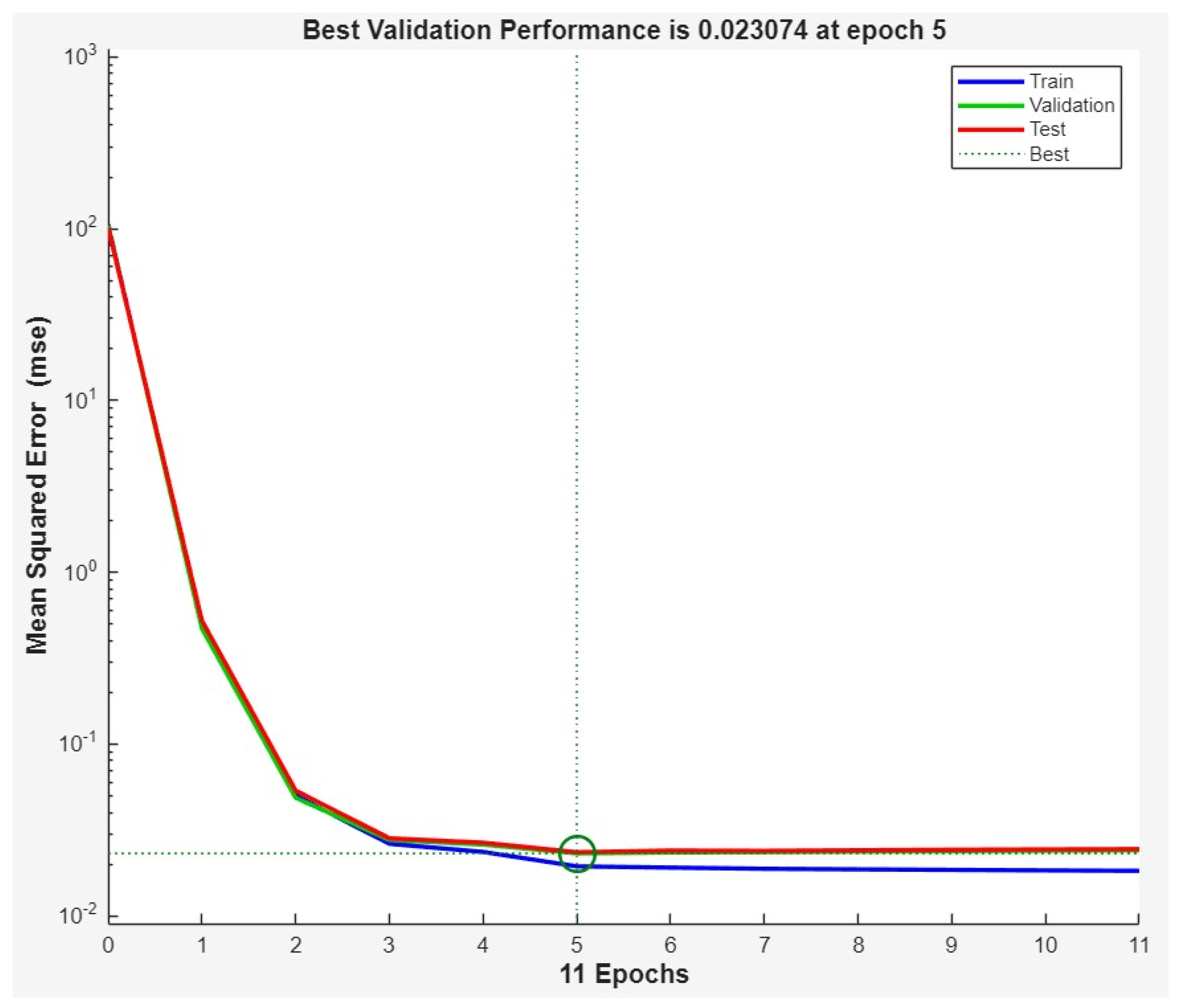
  Levenberg–Marquardt typically stopped within a dozen or so epochs, suggesting rapid convergence (e.g., 11 epochs for 200 neurons).

  ○

  Scaled Conjugate Gradient required a greater number of epochs (e.g., 158 epochs for 10 neurons), confirming its slower learning rate.

• Analysis of Gradient and Mu Parameter

  ○

  Levenberg–Marquardt had relatively high gradient values (e.g., 0.0984 for 80 neurons), suggesting fast weight adjustments.

  ○

  Bayesian Regularization exhibited the smallest gradient values (e.g., 6.89⁻⁵ for 10 neurons), indicating stable and slow training.

  ○

  Mu (regularization parameter for LM) remained low in most cases, suggesting a well-optimized training process.

The best performance (lowest MSE and highest R) was obtained using the Levenberg–Marquardt algorithm with 200 neurons. Bayesian Regularization ensured stable learning but required more epochs. Scaled Conjugate Gradient performed the worst, requiring more epochs and resulting in higher MSE. A larger number of neurons (200) improved results, but models with 50–100 neurons also performed well. Levenberg–Marquardt is the most efficient algorithm, converging quickly and delivering the best results.

Depending on user requirements, Levenberg–Marquardt can be chosen for speed, while Bayesian Regularization is preferable for greater stability and regularization.

The best performance was conducted for model no. 12. The structure of the model is presented below (Figure 5).

Figure 6 presents three plots that describe key metrics during the training process of a neural network. The gradient value decreases over epochs, indicating that the model is converging. At epoch 11, the gradient reaches 0.010657, suggesting a small update in weights and an optimized learning process. The logarithmic scale of the y-axis shows an initial rapid decrease, followed by a more stable gradient reduction, indicating controlled learning.

The parameter Mu (µ) represents the adaptive learning rate for the Levenberg–Marquardt algorithm. Initially, Mu decreases, indicating that the network is adjusting to a more optimal learning rate. Around epoch 5, Mu reaches its minimum and then increases slightly before stabilizing at 1⁻⁵ at epoch 11. This behavior suggests that the network is fine-tuning its learning rate to balance between convergence and avoiding overfitting.

Validation checks monitor when the validation error increases over consecutive epochs. At epoch 11, the number of validation checks reaches 6, meaning that for 6 consecutive epochs, the validation error did not improve. This is a stopping criterion in early stopping mechanisms, indicating that further training might lead to overfitting (Figure 7).

The training process of the neural network is well-regulated. The stopping at epoch 11 is appropriate, as continued training might not improve validation performance and could lead to overfitting. The model appears to be properly trained and optimized within this training phase.

Figure 8 presents four scatter plots, each displaying the relationship between the target values and the model’s output values for different datasets: training, validation, test, and all combined. Here is an interpretation of the results:

• Training Set—The scatter plot shows the correlation between the target and output values for the training dataset. The regression equation is approximate: Output ≈ 0.93 × Target + 0.95. The coefficient of determination (R = 0.96634) suggests a strong correlation, indicating that the model fits the training data well. The data points align closely with the ideal line Y = T (dashed line), with minor deviations.
• Validation Set—This plot represents the validation dataset. The regression equation: Output ≈ 0.92 × Target + 1.1. The correlation coefficient (R = 0.95993) is slightly lower than in the training set but still indicates a good model fit. The data points closely follow the ideal line, demonstrating that the model generalizes well on unseen validation data.
• Test Set—This scatter plot evaluates the model’s performance on the test dataset. The regression equation: Output ≈ 0.91 × Target + 1.2. The correlation coefficient (R = 0.96024) is similar to the validation set, suggesting that the model maintains performance when tested on unseen data.
• Overall Performance—This plot represents the combined results from all datasets (training, validation, and test). The regression equation: Output ≈ 0.92 × Target + 1. The correlation coefficient (R = 0.96445) suggests that the model performs consistently across all data. The correlation values (R > 0.95) indicate a high degree of accuracy in predictions. There is good generalization across validation and test sets, implying minimal overfitting.

Figure 8. Regression plot for model no. 12.

Figure 8. Regression plot for model no. 12.

Figure 9 presents an error histogram (differences between target values and outputs) for a model, likely a neural network, divided into 20 bins. The yellow line marks the zero-error value, serving as a reference point for an ideal model. The concentration of values around this line suggests good model performance, though some deviations exist. Here are the key insights from the analysis: errors range from approximately −0.3065 to 0.2916.

The distribution is centred around zero, suggesting that the model is well-calibrated, but some deviations exist. The largest errors appear at certain peaks, which may indicate that the model struggles to predict specific values.

The model demonstrates good predictive performance, but some errors may require further optimization, such as fine-tuning hyperparameters or improving the dataset.

4. Model Implementation and Results

As a result of implementing the developed mathematical model, a software application (system) was created to determine fuel consumption standards in real-time, forecast fuel consumption on specific routes for individual trips, and predict optimal standards based on the analysis of previously entered data. An additional advantage of the program is its ability to identify vehicles that deviate from fuel consumption standards, allowing for systematic selection of the most suitable fleet for a given route. Furthermore, the reporting module identifies drivers with significantly higher or lower fuel consumption compared to others, enabling the identification of drivers needing training in economical driving and those potentially involved in fuel theft—an unfortunate but possible occurrence.

The system has a modular structure, making it more intuitive to use and allowing for future development and the addition of new modules. The system comprises five main modules, each divided into sections.

• Route Management Module

This module enables input of key route-related information.

• Route Types Section: handles the input of additional correction coefficients for routes. These coefficients go beyond distinguishing between urban and non-urban routes, as the system automatically identifies route types based on average driving speed to match the fuel consumption specified by the manufacturer. The correction coefficient in this section allows for further adjustment of fuel consumption forecasts, accounting for factors such as uphill driving, poor road conditions, and traffic congestion.
• Routes Section: provides a detailed description of routes, including the name, length, number of stops, and additional parameters such as traffic lights, curves, speed bumps, and route type. The route type corresponds to the correction coefficient defined in the previous section.

• Vehicle Management Module

This module manages the company fleet.

• Vehicle Brands Section: records technical data for groups of vehicles, including brand, fuel consumption at idle, in urban and non-urban cycles, curb weight, and gross weight.
• Vehicles Section: captures individual vehicle details such as year of manufacture, mileage, license plate number, seating and standing capacity, and assigns the vehicle to its corresponding brand.

• Driver Management Module

This module consists of sections for driver style and personal data.

• Driving Style Section: assigns a correction coefficient based on driving style, which significantly impacts fuel consumption. The correction coefficient ranges from 0.9 to 1.3, underscoring the importance of economical driving skills.
• Driver Data Section: includes personal information such as name, address, license issue date, number of collisions, and the driver’s associated driving style from the previous section.

• Trip Management Module

This single-section module consolidates data from all other modules. It allows manual entry of trip details, including the following:

• Date of trip;
• Departure and arrival times;
• Heating or air conditioning settings;
• Initial and external temperatures (not used in calculations in the current version but prepared for future system enhancements);
• Total idling time;
• Actual fuel consumption.

It also links the trip with the corresponding route, vehicle, and driver data, forming a relational structure.

• Reporting Module

This is the primary module for creating reports and assigning fuel consumption standards. After selecting a report for a route, driver, or vehicle, the system displays a summary, including the following:

• Route details: name, type, length, number of stops, and additional parameters.
• Selected date or time range, if specified, or a note indicating that the report includes all trips in the database.

The system generates a table (Figure 10) with the following columns:

• Date, departure, and arrival times;
• Vehicle registration number;
• Driver name;
• Actual fuel consumption for the trip;
• System-calculated fuel consumption;
• User-input standard.

Figure 10. Example screenshot of a route report.

Figure 10. Example screenshot of a route report.

The standard proposed by the system is not binding, as it can always be modified by the system administrator. The value can be increased for a more lenient fuel policy or decreased for a stricter policy. However, it is not recommended to reduce the standard excessively, as this could result in setting a standard that is realistically unattainable. The final decision-making factor remains the human managing the system, who must determine the appropriate standard.

The developed system serves as an auxiliary and advisory tool. It highlights areas requiring attention, forecasts real-time fuel consumption, and presents results. However, the ultimate interpretation and decision making always rest with the human operator.

The system highlights deviations from the standard, identifying trips where actual fuel consumption exceeds the forecasted value.

In the “calculated consumption” column, fields where the calculated fuel consumption is less than the actual consumption are highlighted in dark blue. These highlights are independent of the established standard, allowing immediate identification of possible fuel overuse. If a standard has been introduced, the “actual consumption” column undergoes automatic analysis and verification against the entered standard.

In cases of exceedances, the table cells are marked with an appropriate color based on the level of the exceedance. The darker the red, the greater the deviation from the standard. A legend below the table indicates the levels of exceedance and their corresponding colors:

• 0.2% exceedance: light yellow;
• 5% exceedance: dark yellow;
• 10% exceedance: orange;
• 20% exceedance: light red;
• 50% exceedance: dark red.

The use of a color-coded scale makes the summary more visually clear, allowing quick identification of major exceedances while also drawing attention to less significant ones marked in lighter colors. Minor exceedances may often be attributed to additional driving challenges or dynamic driving and can generally be disregarded. However, exceedances marked in orange or red may indicate unusual problems such as the following:

• Forced stops;
• Traffic congestion;
• Road collisions along the route;
• Overloaded vehicles;
• Excessive use of heating or air conditioning;
• Potential fuel theft.

For recurring exceedances at similar times, it is recommended to generate an additional report limited to a specific time frame. This helps to visualize the exceedances more clearly and determine if they result from recurring patterns, such as peak hours, or if they are isolated incidents caused by other factors.

The developed model was analyzed by the prediction error. The results are presented in Figure 11.

In a report for a specific route, another potential issue with exceeding standards may arise: varying fuel consumption between vehicles of different brands. This problem is illustrated by a chart (Figure 12), which is also included as part of the report.

The graph is always automatically generated for each report. In the attached example, you can see significant differences in the amount of fuel used. When comparing them with vehicles and drivers serving a given trip, you can see that the increased fuel consumption is associated with another vehicle and driver. In such a case, it is recommended to swap the drivers driving the vehicles and continue to observe the results. If the norm is still exceeded with another vehicle, you can conclude that this is due to a lack of economical driving skills; otherwise, when the swap does not show a difference, it is obvious that the reason for the overburn is the vehicle, which in turn may be in poor technical condition. Based on these conclusions, you can take appropriate steps such as driver training, vehicle repair, or purchase of a new vehicle when more economical. In Figure 11, you can also see a jump in actual fuel consumption of about 2 liters for route no. 19. Such jumps can be significant because if they are repeated for routes operated by the same driver, they can mean fuel theft. Therefore, you should pay special attention to such exceedances. In such cases, it is a good idea to make an additional report for the driver and pay attention to their exceedances. Both on the graph and in the table, you can see jumps in fuel consumption.

5. Conclusions

The developed and discussed system is designed to determine optimal fuel standards, assist in managing these standards, and identify discrepancies and exceedances. Fuel consumption by vehicles constitutes a significant portion of the overall costs incurred by transportation companies, making rational management and control of fuel consumption critical. This need becomes even more pronounced with larger enterprises.

It is not feasible to oversee this process solely through human effort due to the vast amount of information that must be considered and the number of calculations required to accurately estimate fuel consumption. Managing public transportation enterprises would require a large department dedicated solely to this task. However, current technological advancements enable the replacement of such labor-intensive efforts with advisory systems. These systems process and analyze input data in real time.

The system developed and discussed in this publication offers one of the possible ways to optimize fuel consumption standards. By inputting data on routes, vehicles, drivers, and individual trips—essentially a process of “teaching” the database—the system performs calculations to predict what the vehicle’s fuel consumption should be and conducts comparative analysis between the calculated and actual fuel usage. The system generates real-time reports based on user-defined criteria, enabling ongoing fuel consumption monitoring.

By implementing this system, it is possible to draw informed conclusions and take appropriate actions. Moreover, it allows for the improvement of the weakest links that contribute to increased fuel consumption in the enterprise and offers the following advantages:

• Identifying vehicles with excessive fuel consumption;
• Determining the most economical configuration of vehicles for a given route;
• Identifying drivers who lack skills in economical driving;
• Highlighting drivers who excel in fuel-efficient driving;
• Pinpointing times of the day with the highest congestion on routes;
• Detecting potential cases of fuel theft.

As demonstrated, there are numerous benefits to introducing such systems into an enterprise. Over time, their use can lead to improved operations, optimized solutions, and, consequently, reduced overall operating costs for the entire company.

The developed ANN model enables the prediction of the fuel consumption for regular lines city buses regarding transport parameters like the number of bus stops, traffic jams, number of passengers, ambient temperature, and vehicle technical state. Using this model helps to analyze drivers with low skills of eco-driving or dishonest drivers stealing fuel. Implementation of the proposed system helps to make useful statistics regarding the drivers, vehicles, and routes. Taking into account these benefits, it will be possible to reduce unnecessary costs for companies.

References

- Flakiewicz, W. Systemy Informacyjne w Zarządzaniu: (Uwarunkowania, Technologie, Rodzaje); Wydawnictwo C.H. Beck: Warsaw, Poland, 2002; Volume 7, ISBN 9772081415. [Google Scholar]
- Jarzmik, K.; Jedynak, M.; Sowa, A. Komputerowy System Wspomagania Gospodarki Paliwami Płynnymi w Przedsiębiorstwie Komunikacyjnym. Probl. Eksploat. 1999, 3, 65–78. [Google Scholar]
- Gazewski, T. Jak Zachować Nominalne Zużycie Paliwa; Wydawnictwa Komunikacji i Łączności: Warsaw, Poland, 1990. [Google Scholar]
- Hebda, M. Eksploatacja Samochodów; Wydaw. Inst. Technologii Eksploatacji-PIB: Radom, Poland, 2005. [Google Scholar]
- Niziński, S.; Michalski, R. Utrzymanie Pojazdów i Maszyn; Wydaw. Inst. Technologii Eksploatacji-PIB: Olsztyn, Poland, 2007. [Google Scholar]
- Ubysz, A. Problem “niedoliczenia” W Programie Eko-Drive’05 Przebiegowego Zużycia Paliwa w Samochodzie Na Krótkich Trasach Przejazdu. Probl. Transp. 2007, 3, 51–61. [Google Scholar]
- Liu, T.; Meidani, H. Neural Network Surrogate Models for Aerodynamic Analysis in Truck Platoons: Implications on Autonomous Freight Delivery. Int. J. Transp. Sci. Technol. 2024, 16, 234–243. [Google Scholar] [CrossRef]
- Mustafa, A.; Faisal, S.; Singh, J.; Rezki, B.; Kumar, K.; Moholkar, V.S.; Kutlu, O.; Aboulmagd, A.; Khamees Thabet, H.; El-Bahy, Z.M.; et al. Converting Lignocellulosic Biomass into Valuable End Products for Decentralized Energy Solutions: A Comprehensive Overview. Sustain. Energy Technol. Assess. 2024, 72, 104065. [Google Scholar] [CrossRef]
- Mobasshir, M.; Pachauri, P.; Kumari, P.; Khan, F.; Equbal, A.; Khan, O.; Parvez, M.; Ahamad, T.; Ahmad, S. Analyzing Vehicle Emissions Using a Hybrid Machine Learning Approach Using Weighted Average Based K-Means Clustering for Sustainable Transportation Decision-Making. Green Technol. Sustain. 2025, 3, 100163. [Google Scholar] [CrossRef]
- Komnos, D.; Smit, R.; Ntziachristos, L.; Fontaras, G. A Comparative Analysis of Car Fleet Efficiency Evolution in Europe and Australia Insights on Policy Influence. J. Environ. Manag. 2025, 373, 123313. [Google Scholar] [CrossRef]
- Ahmat, N.; Christopher, S.; Saputra, J.; Sukemi, M.N.; Nawawi, M.N. The Impact of Energy Consumption, Economic Growth, and Non-Renewable Energy on Carbon Dioxide Emission in Malaysia. Int. J. Energy Econ. Policy 2025, 15, 143–152. [Google Scholar] [CrossRef]
- Sharma, D.; Roul, R.K. Intelligent Traffic Congestion Classification Framework. SN Comput. Sci. 2025, 6, 49. [Google Scholar] [CrossRef]
- Tan, M.; Hu, C.; Chen, J.; Wang, L.; Li, Z. Multi-Node Load Forecasting Based on Multi-Task Learning with Modal Feature Extraction. Eng. Appl. Artif. Intell. 2022, 112, 104856. [Google Scholar] [CrossRef]
- Brand, C.; Marsden, G.; Anable, J.L.; Dixon, J.; Barrett, J. Achieving Deep Transport Energy Demand Reductions in the United Kingdom. Renew. Sustain. Energy Rev. 2025, 207, 114941. [Google Scholar] [CrossRef]
- Oweh, S.O.; Aigba, P.A.; Samuel, O.D.; Oyekale, J.; Abam, F.I.; Veza, I.; Enweremadu, C.C.; Der, O.; Ercetin, A.; Sener, R. Improving Productivity at a Marble Processing Plant Through Energy and Exergy Analysis. Sustainability 2024, 16, 11233. [Google Scholar] [CrossRef]
- Zaręba, M.; Danek, T. Analysis of Air Pollution Migration during COVID-19 Lockdown in Krakow, Poland. Aerosol Air Qual. Res. 2022, 22, 210275. [Google Scholar] [CrossRef]
- Adamović, D.; Adamović, S.; Čepić, Z.; Morača, S.; Mihailović, A.; Mijailović, I.; Stošić, M. Possibilities of Improving the Emission Characteristics of Passenger Cars by Controlling the Concentration Levels of Combustion-Generated BTEX Components. Sustainability 2024, 16, 11033. [Google Scholar] [CrossRef]
- Zhang, C.; Ma, Y.; Li, Z.; Han, L.; Xiang, C.; Wei, Z. Fuel-Economy-Optimal Power Regulation for a Twin-Shaft Turboshaft Engine Power Generation Unit Based on High-Pressure Shaft Power Injection and Variable Shaft Speed. Energy 2024, 309, 133153. [Google Scholar] [CrossRef]
- Pandey, A.; Pandey, G.; Mishra, R.K. Evaluating Exhaust Emissions from Heterogeneous Car Fleet through Real-Time Field-Generated Dataset. Atmos. Pollut. Res. 2024, 15, 102232. [Google Scholar] [CrossRef]
- Mane, V.; Vishal, P.; Nikita, P.; Iyer, N.C.; Ashwini, K. Model-Based Design Technique to Monitor Vehicle Exhaust Emissions. Lect. Notes Netw. Syst. 2023, 401, 797–803. [Google Scholar] [CrossRef]
- Kaczor, G.; Zając, G. Analiza Niezawodności Wtryskiwaczy. Czas. Tech. 2012, 109, 327–334. [Google Scholar]
- Ubysz, A. Prognozowanie Zużycia Paliwa w Samochodzie Osobowym w Ruchu Rzeczywistym. Czas. Tech. 2008, 105, 209–217. [Google Scholar]
- Szypulski, P. Siedem Sposobów Na Niższe Spalanie. Co Działa, Co Nie Działa, a Co Ma Niebezpieczne Skutki Uboczne? Available online: https://www.auto-swiat.pl/porady/eksploatacja/sposoby-na-nizsze-spalanie-jak-jezdzic-taniej-skutki-uboczne-oszczedzania-paliwa/lfplz2v (accessed on 15 January 2025).
- Feng, C.; Shao, L.; Wang, J.; Zhang, Y.; Wen, F. Short-Term Load Forecasting of Distribution Transformer Supply Zones Based on Federated Model-Agnostic Meta Learning. IEEE Trans. Power Syst. 2025, 40, 31–45. [Google Scholar] [CrossRef]