Exploring the Driving Factors of Land Use Change and Spatial Distribution in Coastal Cities: A Case Study of Xiamen City

Abstract

This study focuses on the coastal city of Xiamen, examining the factors and driving mechanisms influencing land use changes and spatial patterns. Spatial logistic regression and Statistical Package for the Social Sciences (SPSS) software were employed using grid data with a resolution of 100m to analyze the spatial relationships between six driving factors (such as elevation and slope) and five land use types within the study area. Regression models were established for each factor, and all Relative Operating Characteristic (ROC) tests were passed. Based on the results of the logistic regression analysis, land use changes and spatial distribution were simulated using the updated Conversion of Land Use and its Effects (CLUE) model so as to validate the driving mechanisms. The findings indicate that the six driving factors effectively explain the spatial patterns of land use in the study area. The distance to the coastline is the primary influencing factor in the evolution of spatial patterns, particularly impacting built-up land and farmland, while for forest land, slope is the main factor affecting the spatial distribution. The simulation and accuracy analysis revealed an overall simulation accuracy ranging from 73% to 90.1%, demonstrating that the selected driving factors have effective explanatory power for the spatial distribution of land use. Thus, this study’s results provide valuable insights into the complexity of land use changes and serve as a reference for relevant departments in land use management and planning.

1. Introduction

Human interventions in land use are a major driver of changes in various surface processes [1,2]. Significant alterations in the structure, processes, and patterns of land use can lead to a range of ecological and environmental issues, such as regional soil erosion and land degradation. Therefore, studying land use changes is central to resource management and planning and has become a focal point in global environmental change and sustainable development research [3,4]. Investigating the driving factors and mechanisms behind land use changes is crucial for understanding the dynamic patterns of urban development and its environmental impacts, as well as simulating and predicting future land use changes [5,6].

In recent years, experts and scholars have conducted extensive research on the driving mechanisms of land use changes, as well as the optimization of land use changes, progressing from theoretical analysis to quantitative design, static calculations to dynamic simulations, and single-objective to multi-scenario approaches. This has led to the development of a variety of land use change simulation models [7,8]. Quantitative prediction models include the Markov, regression analysis, system dynamics, grey prediction, and neural network models [9]. Spatial simulation models include the cellular automata model [10], agent-based model [11], and CLUE-S (conversion of land use and its effects at a small regional extent) model [12]. Some scholars have also explored hybrid models that combine quantitative prediction with spatial simulation [13]. Compared to other models, the CLUE-S model is particularly noteworthy for its ability to quantitatively analyze the impacts of natural, social, and economic factors on land use changes. It accounts for the competitive relationships between different land use types and can incorporate quantitative prediction models into its framework to comprehensively simulate land use change patterns in various scenarios.

Thus, CLUE-S stands out as a comprehensive tool capable of integrating the impacts of human, socio-economic, and natural environmental drivers on land use changes [14]. It is the ideal model for studying land use changes [15]. Consequently, the CLUE-S model has seen widespread application [16,17,18,19]. In recent research using the CLUE-S model, Da Lü posited that the varying relationships between land use changes and their driving forces can provide valuable insights for predicting land use changes in different regions [20]. Guitang Liao attempted to incorporate regional indicators to improve the model’s accuracy in studies across multiple ecological regions [21]. Ping Zhang combined CLUE-S with the Soil and Water Assessment Tool (SWAT) to effectively assess non-point-source pollution in different scenarios [22]. The Dyna-CLUE model, as the most recent modified version of CLUE-S, represents an advancement in simulations of land use spatial patterns through summarizing and quantitatively analyzing the interactions among land uses and different factors such as natural and social–economic aspects. Considering that the CLUE-S (conversion of land use and its effects at a small regional extent) model is designed for small regions, in this research, we employed its most recent version, Dyna-CLUE, to detect the possible driving factors for the small city of Xiamen, which as a total area of 1700.61 km² (including administrative sea areas).

Since the 1980s, China has experienced rapid industrialization and urbanization due to reforms and opening up [23,24,25]. The urbanization rate, which was estimated at 36.2% in the 2000 census, had risen to 63.89% by the 2020 census. Xiamen, one of China’s five special economic zones established after the reforms, has seen rapid urbanization and economic development, leading the nation in this regard and positively influencing the surrounding areas, especially between 1989 and 2018. In April 1988, the State Council approved Xiamen as a separately planned city, granting it economic management authority equivalent to that of a province. In May 1989, the State Council approved the establishment of Taiwan investment zones in the Xiamen Special Economic Zone (Xiamen Island) and Xinglin and Haicang areas within Xiamen city. By 2020, Xiamen’s urbanization rate reached an impressive 89.41%, even surpassing Shanghai’s 89.3%. However, Xiamen’s rapid urbanization has resulted in the significant conversion of its watershed and farmland into built-up land.

For a better understanding of the spatial distribution and changes in land use in Xiamen city, as well as better management and planning, a related analysis of driving forces and mechanisms is necessary [26]. For the identification of possible factors, global and local studies on coastal cities were reviewed [27,28,29,30]; specifically, study areas not far from Xiamen city were carefully examined [30,31]. Liao proposed an urban model that integrates multiple approaches such as ordered weighted averaging, binary logistic regression, and cellular automata to simulate future patterns under different ecological constraints in order to accurately determine Xiamen’s spatial evolution [32,33]. However, Liao’s research on land use changes is mainly related to built-up land. Similarly, we previously conducted a study on built-up areas, mainly focusing on the distance to the coastline [26]. Based on these studies [26,32,33], in this paper, we aim to further investigate the factors influencing the spatial distribution of all land use types in the study area. The scope of influencing factors is expanded beyond the coastline to include additional variables, such as the distance to town centers and district centers [32,33].

This study investigates the spatiotemporal characteristics of land use changes in Xiamen from 1989 to 2018. Unlike previous studies focused on single land use types or periods, this study comprehensively analyzes the relationships between various driving factors and all land use types for three phases (1989–2000, 2000–2010, and 2010-2018), establishing regression models for each factor using the logistic regression model and SPSS 16.0 software. After quantifying the impact of six driving factors on the spatial distribution of land use in Xiamen, in this study, we ranked the performance of each factor and identified the primary factors influencing land use changes. Furthermore, the Dyna-CLUE model was used to simulate land use changes for the three phases (1989–2000, 2000–2010, and 2010–2018), and the accuracy of the simulation was determined through Grid Calculator in ArcGIS 10.0, confirming the reliability of the driving factors. Based on such analyses, this research provides a foundation for simulating land use distribution under various planning scenarios, offering scientific decision-making support for regional sustainable development, efficient land resource utilization, and coastal eco-environmental protection.

2. Methodology

2.1. Study Area, Hypothesis, Data Source and Processing

2.1.1. Study Area

Xiamen city is located in Fujian Province along the southeastern coast of China, situated between 117°53′ E–118°26′ E and 24°23′ N–24°54′ N. The city governs six districts, covering a total area of 1700.61 square kilometers. Xiamen features lower elevation in the east and south and higher elevation in the west and north, while its coastline is extensive and abundant with tidal flats.

After it was established as one of the five special economy zones in the 1980s during the reform and opening-up period, rapid development was initiated in Xiamen, and it gradually became a new hub for economic growth on China’s coast. The speed of industrialization and urbanization further increased when it was approved as a separately planned city by the State Council in April 1988, granting it economic management authority equivalent to that of a province [26]. In May 1989, Taiwan investment zones were approved by the State Council in the Xiamen Special Economic Zone (Xiamen Island) and Xinglin and Haicang areas within Xiamen city. Then, in February 1994, the State Council approved the upgrade of Xiamen’s administrative level to a vice-provincial level, while in June 2010, the State Council approved the expansion of the Xiamen Special Economic Zone to cover the entire city of Xiamen [34].

Thus, between 1989 and 2018, Xiamen experienced rapid industrialization and urbanization, resulting in the significant conversion of other land use types into built-up land. The Seventh National Census in 2020 shows that Xiamen’s urbanization rate reached 89.41%, surpassing the national rate of 63.89% [34,35]. Therefore, 1989–2018 was chosen as the study period, and it was divided into three phases to confirm the possible driving forces.

2.1.2. Observation and Research Hypothesis

As shown in Figure 1, from 1989 to 2018, built-up land in Xiamen city consistently increased, while farmland and watershed areas steadily decreased. Spatially, the increase in built-up land and the decrease in farmland and watershed areas are primarily concentrated in low-lying areas near the coastline both on and off Xiamen Island. Spatially, built-up land in Xiamen city is predominantly concentrated in coastal tidal flat areas.

For spatiotemporal characteristics of the three phases (1989–2000, 2000–2010, and 2010–2018), before 2000, the growth of built-up land was primarily concentrated on the island. By 2010, nearly the entire island, except for the southern mountainous areas, had been converted to built-up land. Rapid urbanization over the past decade has created a substantial demand for land use that the island could no longer meet, leading to significant growth in built-up land off the island. However, these new built-up areas off the island were relatively scattered and fragmented. By 2018, the built-up land off the island had transformed from a scattered pattern to more continuous and densely packed areas. At this point, built-up land was almost entirely concentrated in low-lying areas near the coastline.

For the selection of the possible factors, this study first referred to research on coastal cities in the world and in China [27,28,29,30]. The factors are mainly categorized as natural and socio-economic factors, including various distance factors, soil, temperature, GDP, and population. Similar research on coastal cities or regions, such as Guangzhou and its surrounding areas, influenced the chosen factors, considering that these areas are not far away from Xiamen city (about 500 km). The factors in these studies mainly include population, GDP, and various distances [30,31].

Unlike Guangzhou and its surrounding area, where the urban distribution pattern is greatly affected by rivers, there is no river on Xiamen Island and the rivers on the mainland of Xiamen city are just small brooks. Thus, the distance to rivers factor is excluded, while the coastline was considered as a factor due to the presence of a long coastline in Xiamen city that has greatly affected the urban sprawl [26]. Considering the unavailability of population and GDP data at the town level and that the rough data at the district level would affect the accuracy and results, both of these factors were excluded. Finally, this study considered topographic and distance factors, such as the distance to the road network, built-up areas, and coastline, as possible driving factors, as Liao did in simulations of Xiamen [32,33]. However, in contrast to Liao and Gong [31,32], this study combines various road networks, and the distance to the city center is changed to the distance to the district center, aiming to improve the simulation performance. More detail as to why these factors were specifically considered is introduced in the following [36,37]:

(1)

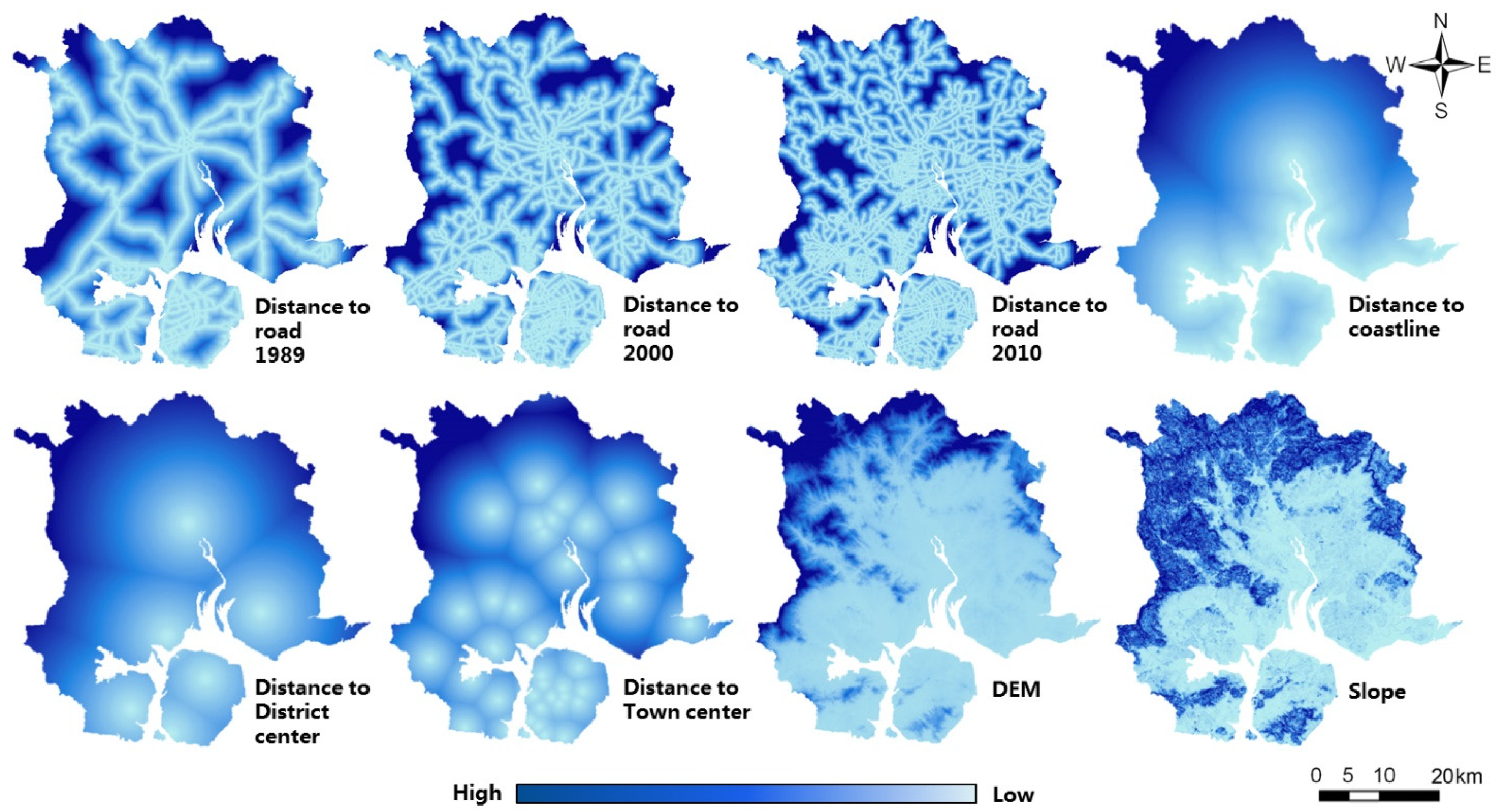
New built-up land expands outward from the original built-up areas. Since the reform and opening-up period, such a distribution may be influenced by the urbanization and industrialization of district centers, along with the structure of port economies and industrial zones [38,39]. Consequently, factors such as the distances to district centers and town centers were selected as possible driving factors for analysis.

(2)

The process of urbanization and industrialization has led to the construction of an extensive road network. The expansion and connectivity of the road network have further influenced surrounding land use changes, facilitating the conversion of farmland into built-up land [40,41]. Thus, the distance to the road network was chosen as a possible driving factor.

(3)

Considering that the district centers are predominantly located in areas not far from the coastline and that the expansion of built-up land and the loss of farmland primarily occur in coastal regions, while forested areas are found further from the coast, the distance to the coastline was selected as a possible driving factor.

(4)

Finally, the terrain elevation and slope likely play a significant role [42,43]. The topography in Xiamen differs from the northwest to the southeast, with higher elevations in the northwest, which is the main area for grasslands and forests [39]. Moving southeast from the low- to mid-elevation mountains and high hills of the northwest, there are low hills, marine plains, and tidal flats. The farmland in low and flat areas has been developed into built-up land previously [43]. Hence, elevation and slope were chosen as possible driving factors.

2.1.3. Data Source and Data Processing

In this research, the land use and elevation data from 1989, 2000, 2010, and 2018 were obtained from the Data Center of the Chinese Academy of Sciences. Based on current land use data and considering the classification standards, as well as the limitations of the Dyna-CLUE model (the area of each land use category must exceed 1% of the study area), the land use data from the study area were initially categorized into five types in ArcGIS: farmland, forest land, built-up land, watersheds, and grassland. Further, the land use vector data were converted into raster data with the polygon-to-raster tool in ArcGIS. Each raster cell indicates the presence (1) or absence (0) of a particular land use type [44,45]. This binary variable serves as the dependent variable for logistic regression. Subsequently, a logistic model was constructed, and a regression analysis was performed.

From the aforementioned observations and hypotheses, six factors were selected as driving variables considering both natural and socio-economic aspects: elevation, slope, distance to roads (DR), distance to town center (DTC), distance to district center (DDC), and distance to coastline (DC). These factors were spatialized accordingly. Specifically, slope data were extracted from DEM files, while the Euclidean Distance was employed to generate spatial files for the other distance-related factors in ArcGIS.

All raster boundaries were unified using the year 2000 as the boundary, which facilitates spatial logistic regression analysis in SPSS and simulations of spatial distribution in Dyna-CLUE. The processing of the driving factors is shown in the following figure (Figure 2).

2.2. Methods

2.2.1. Logistic Regression

Binary logistic regression is one of the most commonly used models in land use analysis [46]. Land use types are employed within the study area as dependent variables and driving factors are employed as independent variables to explore the causal relationships and trends between them. By conducting regression analysis using SPSS 16.0 software on the five land use types and six driving factors, we can obtain the coefficients (β values) and constants of the regression equations for each land use type. The logistic regression model can be written as follows [47]:

$$\log \left(P_{\mathrm{i}}/1-P_{\mathrm{i}}\right)={\beta }_0+{\beta }_1{X}_1+{\beta }_2{X}_2+\cdots +{\beta }_{\mathrm{n}}{X}_{\mathrm{n}}$$

(1)

where P_i is the probability of the occurrence of the considered land use type for a cell, X_n represents the driving factors of each variable, β₀ represents the intercept, and β_n represents the coefficient of each variable.

2.2.2. Dyna-CLUE Model

The Dyna-CLUE model consists of a non-spatial analysis module and a spatial allocation module. The non-spatial analysis module calculates the demand for each land use type within the study area, projecting the required land use quantities for the target year. These annual land use demand files are then input as parameters. Based on the spatial distribution characteristics of land use influence factors, the spatial module iteratively allocates these demands using a raster-based approach, simulating the spatial layout of each land use type [45]. The parameter settings for the Dyna-CLUE model are as follows.

(1)

Restricted Area: The regional constraint file delineates the administrative boundaries of the study area, with large water bodies designated as restricted areas.

(2)

Conversion Rules of Land Use Type: Based on the historical characteristics of land use in the study area for the three phases (1989–2000, 2000–2010, and 2010–2018), the conversion flexibility coefficients for farmland, grassland, forest land, built-up land, and watershed were established [31,48], as well as the transition matrix for simulations (Figure 3). Logistic regression was employed to derive the regression coefficients for the distribution of each land use type relative to the driving factors, thus defining the distribution rules for each land use type.

(3)

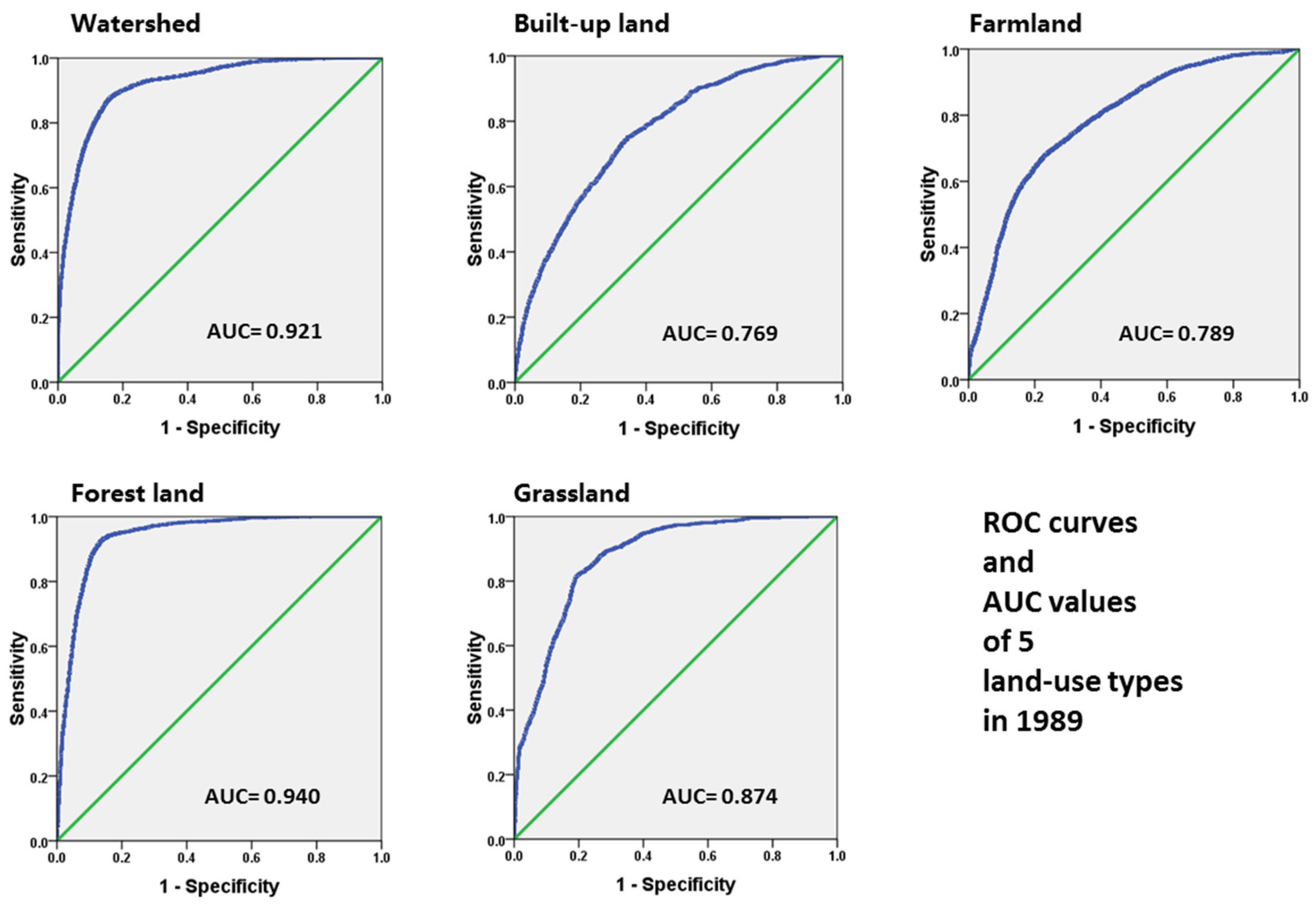
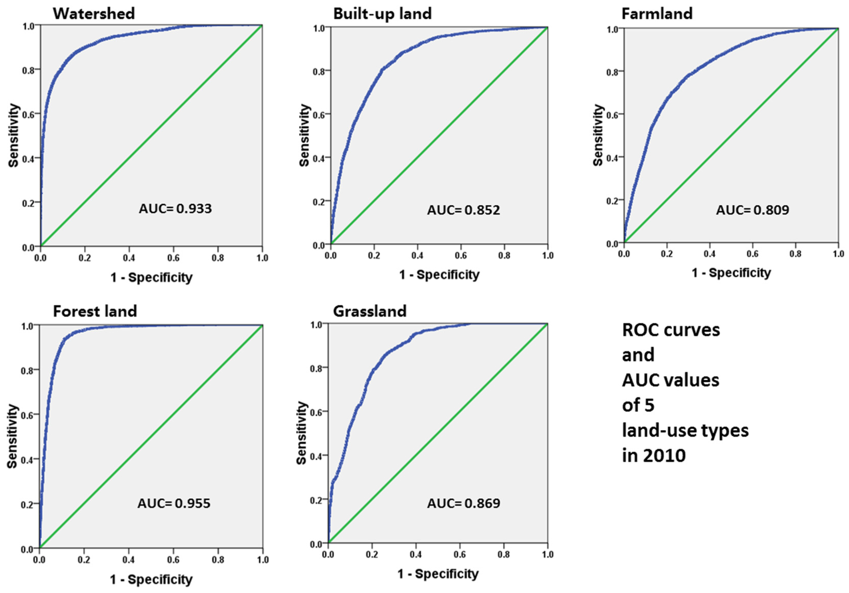
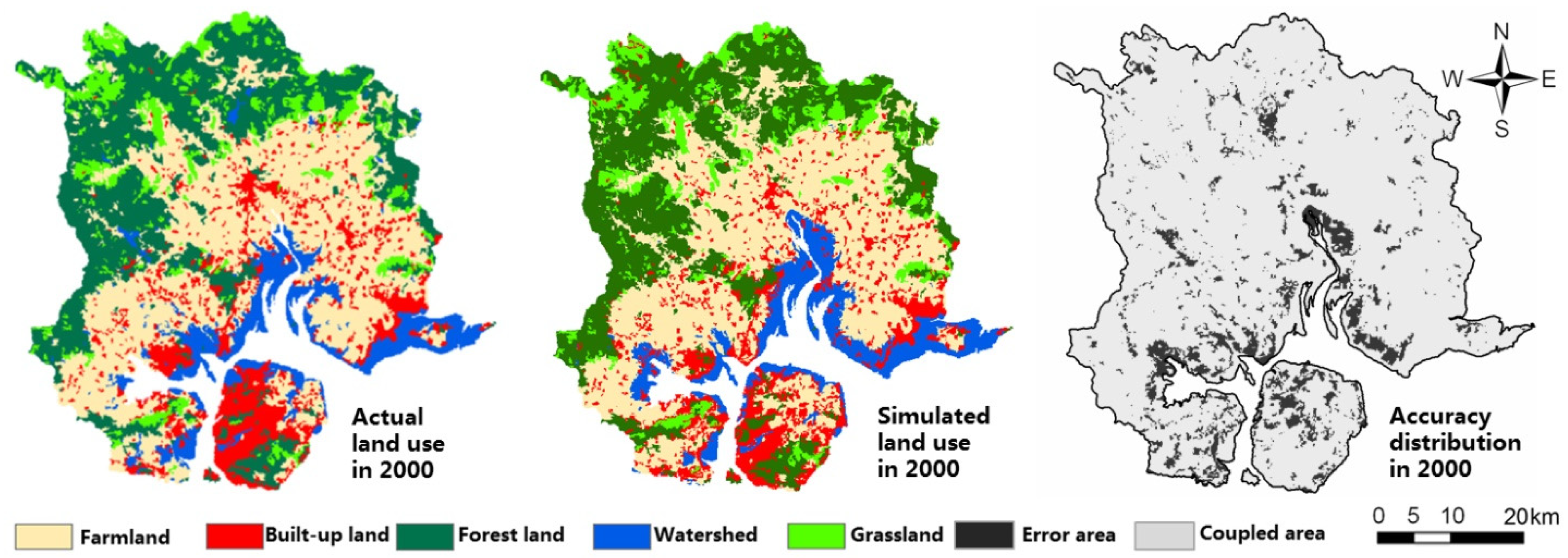
Model Validation: First, the Relative Operating Characteristic (ROC) method was used to validate the logistic regression results [45]. The calculated Area Under the Curve (AUC) of ROC ranges from 0.5 to 1; when the AUC value exceeds 0.7, the selected driving factors are considered to have a good explanatory ability for the land use types and this suggests a better prediction ability and accuracy [45]. Second, the Dyna-CLUE simulation results were validated by spatially overlaying the spatial distribution of simulated land use with the actual observed land use map and calculating the Kappa coefficient to assess the simulation accuracy [49]. A Kappa coefficient of 75% or higher suggests better similarity [50,51,52].

3. Results

3.1. Logistic Regression Results and ROC Test at Each Time Point

As mentioned in the Introduction Section, since the reforms and opening up, rapid urbanization in Xiamen has led to a huge amount of farmland being converted to built-up land. In particular, over the past 30 years (1989–2018), Xiamen’s land use changes exhibited distinct spatial patterns, with built-up land densely concentrated along the coastline and highly overlapping with the road network; see Figure 1. This area is characterized by low elevation and gentle slopes, while forest land is primarily found in the northern mountainous regions.

Additionally, the city has positioned itself as a major international tourist destination, rich in historical and cultural tourism resources. Therefore, achieving harmonious development between the socio-economic sector and the ecological environment is of paramount importance.

Raster maps of the six selected driving factors were created in ArcGIS and then converted into single-column data using the convert.exe tool included in the Dyna-CLUE model. The data were then imported into SPSS for regression analysis to calculate the relationships between the driving factors and each land use type. The regression results were subsequently validated using the ROC method.

3.1.1. Logistic Regression in 1989

The coefficient results of the regression analysis and the corresponding ROC values are presented in

Table 1. The logistic regression coefficient and AUC values of different land use types in 1989.

1989	Watershed	Built-Up Land	Farmland	Forest Land	Grassland
DR	3.252	−5.061	−1.49		1.171
DC	−10.493	3.004	9.654	2.998	7.403
DDC	1.984	−2.825	−1.425	1.612	−3.857
DTC	6.207	−4.94	−5.023	−2.21	−2.534
Dem	−3.526	−6.322	−8.67		2.879
Slope	−15.559	1.228	−2.443		0.789
AUC	0.921	0.769	0.789	0.94	0.874

and Figure 4.

In the regression results for this time point, the AUC values for all five land use types are greater than 0.7, indicating that the regression equations effectively explain the relationship between driving factors and land use types. Among these, the spatial distribution of watersheds and forests is explained best, with AUC values of 0.921 and 0.94, respectively. However, the AUC value for built-up land is only 0.769, suggesting the driving factors only weakly explain its spatial variation. This could be due to its more scattered spatial distribution and dynamic characteristics.

In all regression equations, six factors were statistically significant (p < 0.05) with respect to four land use types (watershed, built-up land, farmland, and grassland), while the regression equations for forest land with the road, elevation, and slope factors were not statistically significant (p < 0.05).

More specifically, for the four land use types of built-up land, farmland, forest land, and grassland, the factor with the greatest impact (highest coefficient) is the distance to the coastline, while for the watershed, the factor affecting the water body most is the distance to the town center (β = 6.207).

From the data presented in the table above, it is evident that, in 1989, the distance to the coastline significantly influenced the spatial distribution of land use. This finding aligns with the observed spatial distribution of land use in 1989, wherein built-up land and farmland were primarily located in areas near the coastline, while forests and grasslands were situated in regions farther from the coast.

As mentioned above, the distance to the coastline is the factor that most affects all land use types, except for watershed land. Among these land use types, farmland has the highest coefficient in the regression equation (β = 9.654). In addition, the change in farmland area during the period from 1989 to 2000 was the largest (−4043 ha). This result shows that the distance to the coastline had a significant impact on the land use changes from 1989 to 2000, especially on the transfer of farmland to other land use types such as built-up land.

3.1.2. Logistic Regression in 2000

The coefficient results of the regression analysis and the corresponding ROC values are presented in

Table 2. The logistic regression coefficient and AUC values of different land use types in 2000.

2000	Watershed	Built-Up Land	Farmland	Forest Land	Grassland
DR	10.029	−10.51	−6.211	1.454
DC	−9.23	2.791	8.516	4.165	6.6
DDC	1.201	−2.569		0.896	−3.273
DTC	5.137	−6.678	−3.497	−3.3	−2.29
Dem	−10.456	−3.715	−10.138	0.616	3.792
Slope	−13.255	1.409	−1.355	8.648	0.719
AUC	0.927	0.807	0.801	0.945	0.883

and Figure 5.

In the regression results for the year 2000, the AUC values for all five land use types are greater than 0.8, suggesting that the factors and regression equations effectively explain the spatial distribution of land use types.

There is statistical significance in the regression equation between the six factors and the three land use types of water, built-up land, and forest land (p < 0.05). However, in the regression equation for farmland, the distance to the district center has no statistical significance (p < 0.05), and in the regression equation for grassland, the distance to the road has no statistical significance (p < 0.05).

For the largest coefficients in the year 2000, the distance to the coastline remained the most influential factor for built-up land, farmland, and grassland. For watershed land, the most significant factor was the distance to the road (β = 10.029), while for forest land, the most significant factor was the slope (β = 8.648), followed by the distance to the coastline (β = 4.165). These results indicate that, in 2000, the distance to the coastline generally influenced the spatial distribution of land use. In particular, the spatial distribution of forest land in 2000 exhibited two main characteristics: forest land was located in areas far from the coastline and in mountainous regions with steeper slopes.

Among the three land use types most influenced by the distance to the coastline, the regression equation showed that the coefficient for farmland was the largest (β = 8.516). From 2000 to 2010, farmland experienced the second largest change (−15,119 ha). This result indicates that, similar to the period from 1989 to 2000, the distance to the coastline significantly influenced the conversion of farmland to other land use types.

3.1.3. Logistic Regression in 2010

The coefficient results of the regression analysis and the corresponding AUC values are presented in

Table 3. The logistic regression coefficient and AUC values of different land use types in 2010.

2010	Watershed	Built-Up Land	Farmland	Forest Land	Grassland
DR	15.079	−19.224	−7.608	0.841
DC	−6.408		8.093	3.078	8.388
DDC	1.599	−2.412	0.591	1.521	−4.603
DTC	9.235	−6.471	−4.648	−3.851	−2.409
Dem	−13.215		−8.11	2.513	2.597
Slope	−13.53		−1.809	9.418	0.962
AUC	0.933	0.852	0.809	0.955	0.869

and Figure 6.

Similar to the year 2000, in the regression results for the year 2010, the AUC values for all five land use types are greater than 0.8, suggesting that the factors and regression equations effectively explain the spatial distribution of land use types.

In 2010, the regression equations for watershed, farmland, and forest land showed statistically significant relationships with all six factors (p < 0.05). However, in the regression equation for grassland, the distance to the road was not statistically significant (p < 0.05). Similarly, in the regression equation for built-up land, elevation, slope, and the distance to the coastline were not statistically significant (p < 0.05).

For the largest coefficients, the distance to the coastline remained the most influential factor for farmland and grassland. As in 2000, the most significant factor affecting the watershed was still the distance to the road (β = 15.079). For forest land, the slope remained the most significant factor (β = 9.418), followed by the distance to the coastline (β = 3.078). These results indicate that, in 2010, the factors influencing the spatial distribution of land use were more diverse, with the distance to the coastline showing a slight advantage, significantly impacting two land use types.

The two land use types that were significantly affected by the distance to the coastline exhibited the biggest change in the period of 2010–2018. These results indicate that from 2010 to 2018, the distance to the coastline continued to significantly influence the reduction in farmland and increase in grassland. Analyzing the spatial distribution changes in land use during this period reveals that there was a substantial conversion of farmland to grassland. Such a phenomenon may be attributed to the ongoing migration of the population into urban areas, resulting in the abandonment of farmland, which subsequently became grassland.

3.2. Simulation Results and Accuracy Testing for Each Period

Based on the file settings and land use data of the initial year, Dyna-CLUE software was used to generate the predicted land use files for the target year. These files were converted into raster data using the ASCII to Raster tool in ArcGIS, resulting in the simulated land use distribution for the target year. Further, with the Raster Calculator in ArcGIS, the simulated results were compared with the actual land use data of the target year (see

Table 4. Comparison of actual cells with simulated correct ones and accuracy calculation results using the Kappa test.

Land Use	Watershed	Built-Up Land	Farmland	Forest Land	Grassland	Total Cells (%)
Actual cells in 2000	15,261	21,649	62,407	46,762	15,203	161,282 (100%)
Correct cells in simulated (2000)	11,412	18,030	55,606	45,309	14,969	145,326 (90.1%)
Actual cells in 2010	13,539	40,240	47,288	47,186	13,029	161,282 (100%)
Correct cells in simulated (2010)	9882	25,924	36,191	44,189	10,731	126,917 (78.7%)
Actual cells in 2018	10,586	49,072	17,779	57,834	26,011	161,282 (100%)
Correct cells in simulated (2018)	7411	33,349	7620	48,227	7824	104,431 (64.8%)

); raster cells with a value of 0 indicate correct simulations. The Kappa coefficient was then calculated to interpret the accuracy of the simulation.

3.2.1. Simulation in the Period of 1989–2000

Over this period, the simulation achieved an overall accuracy of 90.1%, with a Kappa coefficient of 87.6% (see Table 4), indicating a high-quality simulation. Therefore, for the study area, it can be concluded that the Dyna-CLUE model effectively simulates land use changes with the selected driving factors. This model can be applied to future land use simulations and optimizations. Spatially, when comparing the actual land use of the target year with the simulated results, the overall distribution of each land use type was consistent (Figure 7). Although there are simulation errors along the coastline, the deviations are not significant.

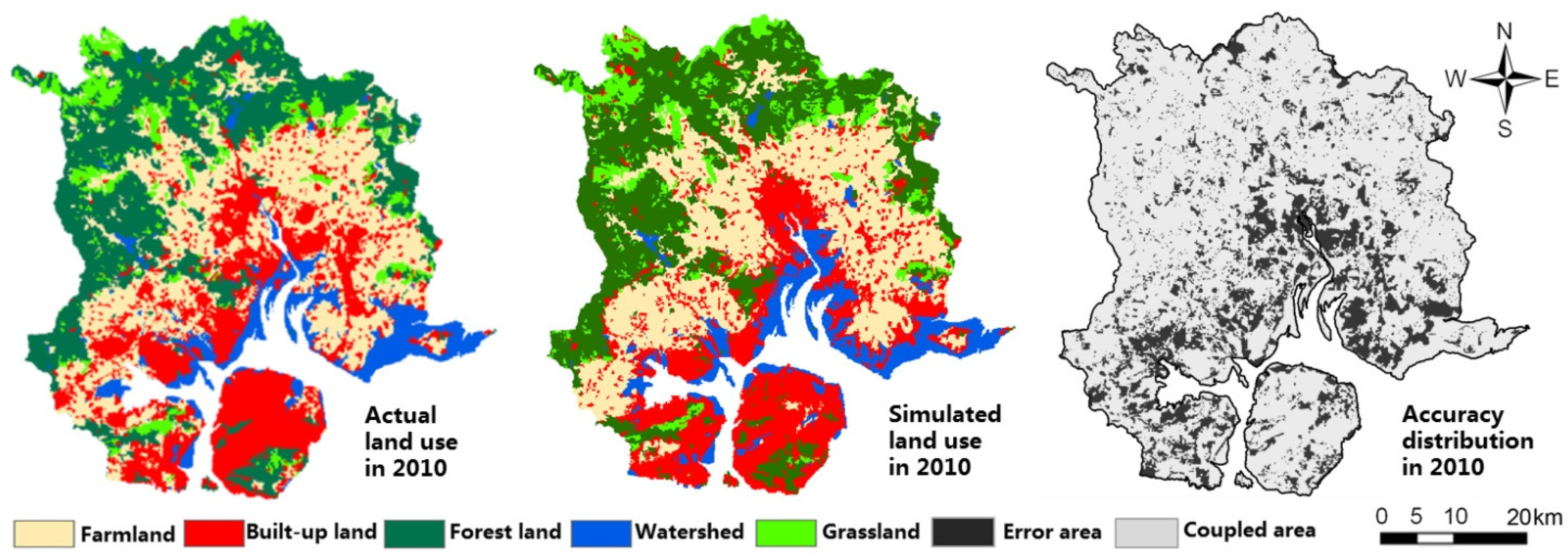
3.2.2. Simulation in the Period of 2000–2010

For this period, the simulation achieved an overall accuracy of 78.7% and a Kappa coefficient of 73.4% (see Table 4), indicating a moderate simulation performance. Spatially, when comparing the actual land use of the target year with the simulated results, the overall distribution of each land use type was consistent (Figure 8). Similar to the previous period, although there are simulation errors along the coastline, the deviation proportion is still low.

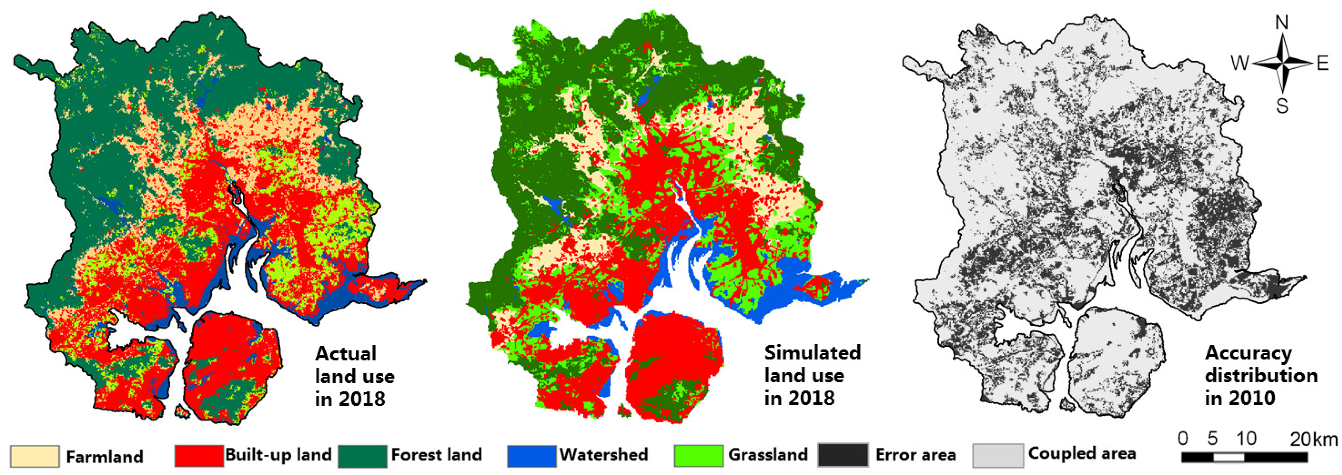
3.2.3. Simulation in the Period of 2010–2018

The simulation for this period achieved an overall accuracy of 64.8% and a Kappa coefficient of 56% (see Table 4), indicating a suboptimal performance. Spatially, when comparing the actual land use of the target year with the simulated results, the overall distribution of each land use type was consistent but with significant deviations (Figure 9). The main factors lowering the accuracy were the precision of grassland and farmland at only 30.1% and 42.9%, respectively. The accuracy of these two land use types is significantly lower than the other three land use types, greatly reducing the overall accuracy and Kappa coefficient. If grassland and the highly correlated farmland were excluded as outliers, the average accuracy for 2010–2018 would be higher (73.8%).

Observations of the spatial distribution of land use from 2010 to 2018 reveal significant changes in grassland distribution. Grassland and farmland represent the largest quantitative change during this period. Specifically, farmland decreased by 29,509 hectares, while grassland increased by 12,982 hectares. Additionally, an overlay analysis of land use types in this period indicates that farmland was primarily converted to grassland after it was converted to built-up land. Consequently, substantial changes in the spatial distribution of grassland not only led to a decline in the accuracy of grassland delineation but also affected the spatial distribution and simulation accuracy of farmland.

4. Discussion

4.1. Land Use Changes, Coastline, and Accuracy

The extent of land use changes has increased over time. The reduction in farmland from 2000 to 2010 was 374% higher than the reduction observed from 1989 to 2000, and the reduction from 2010 to 2018 was 730% higher than that in 1989–2000 [53]. Concurrently, the influence of the coastline on the spatial distribution of land use at each time point diminished, and the accuracy of the simulations progressively decreased.

In 1989, the spatial distribution of the land use categories, excluding watershed areas, was most significantly influenced by their distance from the coastline. Among these, farmland was particularly affected by this factor, in contrast to the other three categories. The regression coefficients for distance to the coastline in the land use category equations are ranked as follows: farmland (9.654) > grassland (7.403) > built-up land (3.004) > forest land (2.998). The overall simulation accuracy for the period from 1989 to 2000 was 90.1%.

By 2000, the land use categories most influenced by the distance to the coastline had reduced to just three: built-up land, farmland, and grassland. Among these three categories, farmland remained the most influenced by the distance to the coastline; the regression coefficients for distance to the coastline in the equations for the three land use categories were ranked as follows: farmland (8.516) > grassland (6.6) > built-up land (2.791). The overall simulation accuracy for the period from 2000 to 2010 was 78.7%, which is a decrease of 11.4% compared to the 1989–2000 period. At this time point, the spatial distribution of forest land was most affected by slope.

By 2010, the land use categories significantly influenced by their distance to the coastline had reduced to two: farmland and grassland. The distance to the coastline was no longer a significant factor affecting built-up land, while slope remained the primary factor influencing the spatial distribution of forest land [42].

The discussion above reveals that the coastline profoundly influenced the land use distribution of the study area over the whole study period [26]. However, it is also noteworthy that as the magnitude of land use changes increased over subsequent periods, the influence of the coastline on the spatial patterns reduced.

Moreover, the decrease in simulation accuracy indicates that greater magnitudes of land use changes pose a challenge to accurately simulating land use dynamics. This difficulty intensifies particularly when land use changes occur abruptly. For instance, from 2010 to 2018, the spatial distribution of grassland shifted from being concentrated in the north to being concentrated in the east and west. This significant alteration in the spatial distribution pattern led to a drastic decrease in the accuracy of grassland simulations during this period, dropping to 30.1%. In contrast, the simulation accuracies for grassland were 98.5% and 82.4% for 1989–2000 and 2000–2010, respectively.

4.2. Rapid Development and Ecological Issues

From 1989 to 2018, Xiamen experienced rapid industrialization and urbanization, during which a large amount of ecological land (farmland, forest land, grassland, and watersheds), especially farmland, was converted into built-up land, resulting in multiple ecological issues [53,54]. As a result of this rapid industrialization and urbanization, there was a significant growth in population coupled with an improvement in living standards. This also led to a sharp increase in food consumption. Thus, the continuous decrease in local farmland means that sufficient foodstuff cannot be produced, with the sustainability of long-term imports from other regions also facing problems [55]. Meanwhile, the development of the economy, along with improvements in living standards, has led to higher concerns and demands regarding the quality of the ecological environment. In addition, Xiamen is an international port and scenic tourist city. All these factors result in significant contradictions between rapid urbanization and industrialization and sustainability goals such as food security and the improved quality of the ecological environment.

Xiamen, a small coastal city with islands, has experienced long-term rapid economic development coupled with huge population growth; however, it now is facing great pressure to promote sustainable development [53,54,55], as well as innovative urban development strategies. One possible approach has been proposed, which is aimed at compact cities with limited urban sprawl boundaries to avoid more reductions in ecological land and to promote a balance between urban and ecological spaces [26,56,57].

Better economic development models also need to be considered to avoid further ecological damage and further develop scenic tourism cities. Among these possible models or strategies, the theory of ecological economy requires that no more ecological land be occupied and that it also be made greener and low-carbon [55].

Xiamen’s development goals are therefore diverse, which poses challenges for land use planning and management; the future spatial distribution of land use should be simulated and optimized based on multiple objectives. This sort of study with complex experiments will be the focus of future research.

4.3. Recommendations for Land Use Management and Urban Planning

A better understanding of the driving factors and coefficients for land use could lead to more accurate simulations of future land use distributions, which would benefit land use planning and management.

In the multiple regression equations for five land use categories and six factors, the factor ranking with regard to number of positive regression coefficients (shown in brackets) is as follows: distance to the coastline (11) > slope (8) > distance to the district centers (7) > distance to roads (6) > elevation (5) > distance to the town center (3).

In addition, for the three time points (1989, 2000, and 2010), the factor ranking with regard to the number of times (in brackets) a factor exhibited the maximum coefficient for each land use type is as follows: distance to the coastline (9)>slope (2)>distance to the road (2)>distance to the town center (1).

The aforementioned ranking results indicate that the distance to the coastline has a dominant influence over land use changes. Therefore, for coastal cities, land use planners should take the influence of the coastline into account. Urban expansion and built-up land may tend to concentrate towards the coastline, resulting in changes in nearby land use categories [43]. However, this dense construction activity may lead to ecological imbalances and extreme alterations in land use category structures [58,59]. Hence, land use planners should prioritize balanced land use and ecological preservation, particularly focusing on coastal ecosystem protection [60].

In addition, not only should ecological land be protected, but abandoned barren lands or grasslands should also be extensively reclaimed to ensure local food security. Surveys show that people tend to prefer living along the coast and in urban areas [61], but this puts pressure on the development of small island cities such as Xiamen. Thus, strategies such as encouraging people to return to rural areas should also be considered to reclaim farmland, develop the rural economy, and ultimately realize rural revitalization [54].

Since people tend to gather in urban and coastal areas, high-quality urban ecosystems should also be constructed through efficient land use planning and management. Thus, policies for the construction of urban ecosystems, such as the strict protection of ecological land and setting up ecological corridors in urban areas, should be planned to encompass the scattered and isolated ecological space within an integrated ecosystem network in the urban space. Such policies, along with urban-area infilling, would not only have a positive effect on the compactness of the city but also improve the urban ecological quality.

4.4. Limitations

In this study, the regression of forest land and the distance to roads was not significant in 1989, and the regression between grassland and the distance to roads was not significant in 2000 or 2010. This finding is similar to those of Hu in their study on Guangzhou [30]. The regression of the distance to roads with grassland and forest land is not significant, indicating that the distance to roads has a low-level impact on natural land use types (such as forest land and grassland). Meanwhile, in both studies, the slope exhibited the highest coefficient [30], indicating that topography has a significant impact on the spatial pattern of land use.

In Hu’s research on Guangzhou, the regression of GDP on three out of six natural land use types (grassland, water area, and wasteland) was not significant. In addition, the regression of population for two natural land use types (forest and water) was also not significant. However, both of these factors were significant for artificial land use (such as farmland and built-up land) [30]. Due to the unavailability of data, in this study, we did not consider the two socio-economic factors of population and GDP. However, further research should focus on the expansion of built-up land and the corresponding occupation of farmland, as considering these two factors would be beneficial.

Based on the exploration of driving factors, land use distributions should be simulated in the future for better land use planning and management. However, such a simulation with multiple scenarios would need to consider many factors and the process would be relatively long. Generally, multiple objectives need to be analyzed and proposed first and then the corresponding complicated set of diverse data needs to be prepared. Next, groups of simulation experiments should be performed, along with a comparison of the results, and finally, optimization decisions should be made. Due to the complexity and length of the process of multi-scenario simulations, this has not been completed yet and is thus not presented in this paper. These multi-scenario simulations will be conducted in the next step of this research.

5. Conclusions

The process of global urbanization is significantly affecting land use and spatial patterns. Understanding the factors driving these changes is crucial for effective land use management and sustainable urban development. This study focuses on Xiamen, a coastal city in China, and analyzes land use changes over 30 years (1989–2018). Spatial logistic regression is used to explore the relationship between influencing factors and spatial patterns of all land use types. In the discussion, the performance of each factor was ranked and the primary factors influencing the land use changes were identified. Further, the Dyna-CLUE model is used to simulate land use changes for three phases (1989–2000, 2000–2010, and 2010–2018) to confirm the impact of these factors.

The results show that at three time points (1989, 2000, and 2010), ROC values in the regression equations exceeded 0.7, demonstrating a strong correlation between driving factors and land use distribution. Out of 90 coefficients across the three periods, only 9 (10%) were insignificant, indicating a strong relationship between the six factors and land use distribution. The simulation accuracy and Kappa coefficient also highlight the robust explanation of land use changes.

The distance to the coastline emerged as the most influential factor on land use changes, followed by slope. This finding has important implications for urban and ecological planning, highlighting the risk of overdevelopment along coastlines and the need for ecological protection strategies.

The simulation results revealed a decline in accuracy as land use changes increased over time. In the first period (1989–2000), the accuracy was 90.1%, with a Kappa coefficient of 0.876, and in the second period (2000–2010), the accuracy dropped to 78.7%, with a Kappa coefficient of 0.734, nearing the threshold of 0.75. The third period (2010–2018) saw a significant decline in accuracy due to drastic changes in grassland distribution, which affected the overall results. This highlights the challenges of simulating land use changes when a land use type, such as grassland, undergoes fundamental spatial shifts.

References

1. Foley Jonathan, A.; DeFries, R.; Asner Gregory, P.; Barford, C.; Bonan, G.; Carpenter Stephen, R.; Chapin, F.S.; Coe Michael, T.; Daily Gretchen, C.; Gibbs Holly, K.; et al. Global consequences of land use. Science 2005, 309, 570–574. [Google Scholar] [CrossRef] [PubMed]
2. Pocewicz, A.; Nielsen-Pincus, M.; Goldberg, C.S.; Johnson, M.H.; Morgan, P.; Force, J.E.; Waits, L.P.; Vierling, L. Predicting land use change: Comparison of models based on landowner surveys and historical land cover trends. Landsc. Ecol. 2008, 23, 195–210. [Google Scholar] [CrossRef]
3. Liu, Y.; Fang, F.; Li, Y. Key issues of land use in China and implications for policy making. Land Use Policy 2014, 40, 6–12. [Google Scholar] [CrossRef]
4. Vizzari, M.; Hilal, M.; Sigura, M.; Antognelli, S.; Joly, D. Urban-rural-natural gradient analysis with CORINE data: An application to the metropolitan France. Landsc. Urban Plan. 2018, 171, 18–29. [Google Scholar] [CrossRef]
5. Ojima, D.; Lavorel, S.; Graumlich, L.; Moran, E. Terrestrial human-environment systems: The future of land research in IGBP II. IGBP Glob. Change Newsl. 2002, 50, 31–34. [Google Scholar]
6. Turner, B.L., II. Toward integrated land-change science: Advances in 1.5 decades of sustained international research on land-use and land-cover change. In Proceedings of the Challenges of a Changing Earth, Global Change Open Science Conference, Amsterdam, The Netherlands, 10–13 July 2001; Springer: Berlin/Heidelberg, Germany, 2001; pp. 21–26. [Google Scholar]
7. White, R.; Engelen, G.; Uljee, I. The use of constrained cellular automata for high resolution modeling of urban land-use dynamics. Environ. Plan. B Plan. Des. 1997, 24, 323–343. [Google Scholar] [CrossRef]
8. Gollnow, F.; Göpel, J.; deBarros Viana Hissa, L.; Schaldach, R.; Lakes, T. Scenarios of land-use change in a deforestation corridor in the Brazilian Amazon: Combining two scales of analysis. Reg. Environ. Change 2018, 18, 143–159. [Google Scholar] [CrossRef]
9. Marsh, G.P. Man and Nature: Or Physical Geography as Modified by Human Action; Charles Scribner: New York, NY, USA, 1869. [Google Scholar]
10. Sharifi, M.A.; van Keulen, H.; van de Toorn, W. Collaborative integrated planning and decision support system for land use planning and policy analysis. Gene 2002, 145, 69–73. [Google Scholar]
11. Agarwal, C.; Green, G.M.; Grove, J.M.; Evans, T.P.; Schweik, C.M. A Review and Assessment of Land-Use Change Models: Dynamics of Space, Time and Human Choice; US Department of Agriculture, Forest Service, Northeastern Research Station: Newton Square, PA, USA, 2002.
12. Simon, R. Swaffield.; John, R. Investigation of attitudes towards the effects of land use change using image editing and Q sort method. Landsc. Urban Plan. 1996, 35, 213–230. [Google Scholar]
13. Hale, I.L.; Wollheim, W.M.; Smith, R.G.; Asbjornsen, H.; Brito, A.F.; Broders, K.; Grandy, A.S.; Rowe, R. A Scale-Explicit Framework for Conceptualizing the Environmental Impacts of Agricultural Land Use Changes. Sustainability 2014, 6, 8432–8451. [Google Scholar] [CrossRef]
14. Salazar, E.; Henríquez, C.; Sliuzas, R.; Qüense, J. Evaluating spatial scenarios for sustainable development in Quito, Ecuador. ISPRS Int. J. Geo-Inf. 2020, 9, 141. [Google Scholar] [CrossRef]
15. Rounsevell, M.D.; Pedroli, B.; Erb, K.-H.; Gramberger, M.; Busck, A.G.; Haberl, H.; Kristensen, S.; Kuemmerle, T.; Lavorel, S.; Lindner, M. Challenges for land system science. Land Use Policy 2012, 29, 899–910. [Google Scholar] [CrossRef]
16. Rong, T.; Zhang, P.; Jing, W.; Zhang, Y.; Li, Y.; Yang, D.; Yang, J.; Chang, H.; Ge, L. Carbon Dioxide Emissions and Their Driving Forces of Land Use Change Based on Economic Contributive Coefficient (ECC) and Ecological Support Coefficient (ESC) in the Lower Yellow River Region (1995–2018). Energies 2020, 13, 2600. [Google Scholar] [CrossRef]
17. Xu, S.; Cheng, Q. Driving forces of land use change in the Tiexi old industrial relocation area, Shenyang, China. Int. J. Environ. Sci. Technol. 2022, 19, 10999–11012. [Google Scholar] [CrossRef]
18. Derakhshan-Babaei, F.; Nosrati, K.; Mirghaed, F.A.; Egli, M. The interrelation between landform, land-use, erosion and soil quality in the Kan catchment of the Tehran province, central Iran. Catena 2021, 204, 105412. [Google Scholar] [CrossRef]
19. Yuen, K.W.; Hanh, T.T.; Quynh, V.D.; Switzer, A.D.; Teng, P.; Lee, H. Interacting effects of land-use change and natural hazards on rice agriculture in the Mekong and Red River deltas in Vietnam. Nat. Hazards Earth Syst. Sci. 2021, 21, 1473–1493. [Google Scholar] [CrossRef]
20. Lü, D.; Gao, G.; Lü, Y.; Ren, Y.; Fu, B. An effective accuracy assessment indicator for credible land use change modeling: Insights from hypothetical and real landscape analyses. Ecol. Indic. 2020, 117, 106552. [Google Scholar] [CrossRef]
21. Liao, G.; He, P.; Gao, X.; Lin, Z.; Huang, C.; Zhou, W.; Deng, Q.; Xu, C.; Deng, L. Land use optimization of rural production–living–ecological space at different scales based on the BP–ANN and CLUE–S models. Ecol. Indic. 2022, 137, 108710. [Google Scholar] [CrossRef]
22. Zhang, P.; Liu, Y.; Pan, Y.; Yu, Z. Land use pattern optimization based on clue-s and swat models for agricultural non-point source pollution control. Math. Comput. Model. 2013, 58, 588–595. [Google Scholar] [CrossRef]
23. Long, Y.; Han, H.; Tu, Y.; Shu, X. Evaluating the effectiveness of urban growth boundaries using human mobility and activity records. Cities 2015, 46, 76–84. [Google Scholar] [CrossRef]
24. Wei Y, D.; Ye X, Y. Urbanization, urban land expansion and environmental change in China. Stoch. Environ. Res. Risk Assess. 2014, 28, 757–765. [Google Scholar] [CrossRef]
25. Yue W, Z.; Fan P, L.; Wei Y, D.; Qi J, G. Economic development, urban expansion, and sustainable development in Shanghai. Stoch. Environ. Res. Risk Assess. 2014, 28, 783–799. [Google Scholar] [CrossRef]
26. Zhang, T. Using Satellite Imagery to Determine Spatiotemporal Patterns of Built-Up Land Use in Relation to the Coastline: An Example from Xiamen, China. J. Coast. Res. 2023, 39, 103–113. [Google Scholar] [CrossRef]
27. Lima, M.L.; Romanelli, A.; Massone, H.E. Assessing groundwater pollution hazard changes under different socio-economic and environmental scenarios in an agricultural watershed. Sci. Total Environ. 2015, 530–531, 333–346. [Google Scholar] [CrossRef]
28. Satiprasad, S.; Indrani, S.; Anirban, D.; Anupam, D.; Pulakesh, D.; Amlanjyoti, K. Future scenarios of land-use suitability modeling for agricultural sustainability in a river basin. J. Clean. Prod. 2018, 205 Pt 1, 313–328. [Google Scholar]
29. Yang, Y.; Bao, W.; Liu, Y. Scenario simulation of land system change in the beijing-tianjin-hebei region. Land Use Policy 2020, 96, 104677. [Google Scholar] [CrossRef]
30. Hu, M.; Wang, Y.; Xia, B.; Jiao, M.; Huang, G. How to balance ecosystem services and economic benefits?—A case study in the pearl river delta, China. J. Environ. Manag. 2020, 271, 110917. [Google Scholar] [CrossRef]
31. Gong, J.; Hu, Z.; Chen, W.; Liu, Y.; Wang, J. Urban expansion dynamics and modes in metropolitan guangzhou, china. Land Use Policy 2018, 72, 100–109. [Google Scholar] [CrossRef]
32. Liao, J.; Shao, G.; Wang, C.; Tang, L.; Qiu, Q. Urban sprawl scenario simulations based on cellular automata and ordered weighted averaging ecological constraints. Ecol. Indic. 2019, 107, 105572. [Google Scholar] [CrossRef]
33. Liao, J.; Tang, L.; Shao, G.; Su, X.; Chen, D.; Xu, T. Incorporation of extended neighborhood mechanisms and its impact on urban land-use cellular automata simulations. Environ. Model. Softw. 2016, 75, 163–175. [Google Scholar] [CrossRef]
34. Xiamen Bureau of Statistics (XBS). 2023. Available online: http://tjj.xm.gov.cn/tjzl/tjsj/tqnj/ (accessed on 1 October 2024).
35. National Bureau of Statistics of China (NBSC). 2023. Available online: https://data.stats.gov.cn/ (accessed on 1 October 2024).
36. Lambin E, F.; Geist H, J.; Lepers, E. Dynamics of land-use and land-cover change in tropical regions. Annu. Rev. Environ. Resour. 2003, 28, 205–241. [Google Scholar] [CrossRef]
37. Turner, B.; Skole, D.; Sanderson, S.; Fischer, G.; Fresco, L.; Leemans, R. Land-Use and Land-Cover Change: Science/Research Plan; IGBP Report No. 35/HDP Report No. 7; IGBP: Stockholm/Sweden/Geneva, Switzerland, 1995. [Google Scholar]
38. Lawler, J.J.; Lewis, D.J.; Nelson, E.; Plantinga, A.J.; Polasky, S.; Withey, J.C.; Helmers, D.P.; Martinuzzi, S.; Pennington, D.; Radeloff, V.C. Projected land-use change impacts on ecosystem services in the United States. Proc. Natl. Acad. Sci. USA 2014, 111, 7492–7497. [Google Scholar] [CrossRef] [PubMed]
39. Waiyasusri, K.; Yumuang, S.; Chotpantarat, S. Monitoring and predicting land use changes in the Huai Thap Salao Watershed area, Uthaithani Province, Thailand, using the CLUE-s model. Environ. Earth Sci. 2016, 75, 533. [Google Scholar] [CrossRef]
40. Jansen, L.J.M.; Bagnoli, M.; Focacci, M. Analysis of land-cover/use change dynamics in Manica Province in Mozambique in a period of transition (1990–2004). For. Ecol. Manag. 2008, 254, 308–326. [Google Scholar] [CrossRef]
41. Liu, J.; Zhang, Z.; Xu, X.; Kuang, W.; Zhou, W.; Zhang, S.; Li, R.; Yan, C.; Yu, D.; Wu, S.; et al. Spatial patterns and driving forces of land use change in China in the early 21st century. Acta Geograph. Sin. 2009, 64, 1411–1420. [Google Scholar] [CrossRef]
42. Wischmeier, W.H.; Smith, D.D. Predicting Rainfall Erosion Losses: A Guide to Conservation Planning; Department of Agriculture, Science and Education Administration: Washington, DC, USA, 1978. [Google Scholar]
43. Du, X.; Jin, X.; Yang, X.; Yang, X.; Zhou, Y. Spatial pattern of land use change and its driving force in Jiangsu province. Int. J. Environ. Res. Public Health 2014, 11, 3215–3232. [Google Scholar] [CrossRef]
44. Verburg, P.H.; Alexander, P.; Evans, T.; Magliocca, N.R.; Malek, Z.; Rounsevell, M.D.; van Vliet, J. Beyond land cover change: Towards a new generation of land use models. Curr. Opin. Environ. Sustain. 2019, 38, 77–85. [Google Scholar] [CrossRef]
45. Pontius, R.G.J.; Boersma, W.; Castella, J.C.; Clarke, K.; Nijs, T.D.; Dietzel, C.; Duan, Z.; Fotsing, E.; Goldstein, N.; Kok, K. Comparing the input, output, and validation maps for several models of land change. Ann. Reg. Sci. 2008, 42, 11–37. [Google Scholar] [CrossRef]
46. Edition, S. Applied logistic regression analysis. Technometrics 2010, 38, 184–186. [Google Scholar]
47. Gobin, A.; Campling, P.; Feyen, J. Logistic modelling to derive agricultural land use determinants: A case study from southeastern Nigeria. Agric. Ecosyst. Environ. 2002, 89, 213–228. [Google Scholar] [CrossRef]
48. Batisani, N.; Yarnal, B. Urban expansion in Centre County, Pennsylvania: Spatial dynamics and landscape transformations. Appl. Geogr. 2009, 29, 235–249. [Google Scholar] [CrossRef]
49. Ren, Y.; Lü, Y.; Comber, A.; Fu, B.; Harris, P.; Wu, L. Spatially explicit simulation of land use/land cover changes: Current coverage and future prospects. Earth-Sci. Rev. 2019, 190, 398–415. [Google Scholar] [CrossRef]
50. Mas, J.-F.; Kolb, M.; Paegelow, M.; Camacho Olmedo, M.T.; Houet, T. Inductive pattern-based land use/cover change models: A comparison of four software packages. Environ. Model. Softw. 2014, 51, 94–111. [Google Scholar] [CrossRef]
51. Zare, M.; Nazari Samani, A.A.; Mohammady, M.; Salmani, H.; Bazrafshan, J. Investigating effects of land use change scenarios on soil erosion using CLUE-s and RUSLE models. Int. J. Environ. Sci. Technol. 2017, 14, 1905–1918. [Google Scholar] [CrossRef]
52. Zheng, F.; Hu, Y. Assessing temporal-spatial land use simulation effects with CLUES and Markov-CA models in Beijing. Environ. Sci. Pollut. Res. 2018, 25, 32231–32245. [Google Scholar] [CrossRef]
53. Zhang, T.; Qu, Y.; Liu, Y.; Yan, G.; Foliente, G. Spatiotemporal Response of Ecosystem Service Values to Land Use Change in Xiamen, China. Sustainability 2022, 14, 12532. [Google Scholar] [CrossRef]
54. Zhang, T.; Sun, W.; Xiao, J.; Yan, G. The impact of land use change on food security under the background of rapid urbanization—A case study of Xiamen city. Environ. Res. Commun. 2024, 6, 105006. [Google Scholar] [CrossRef]
55. Zhang, T.; Tang, L.; Wen, Y.; Wang, C. The development stage of Xiamen city and related environment evolution. J. Environ. Eng. Landsc. Manag. 2022, 30, 350–362. [Google Scholar] [CrossRef]
56. Zhao, J.; Song, Y.; Tang, L.; Shi, L.; Shao, G. China’s cities need to grow in a more compact way. Environ. Sci. Technol. 2011, 45, 8607–8608. [Google Scholar] [CrossRef] [PubMed]
57. Daunt, A.; Inostroza, L.; Hersperger, A.M. The role of spatial planning in land change: An assessment of urban planning and nature conservation efficiency at the southeastern coast of Brazil. Land Use Policy 2021, 111, 105771. [Google Scholar] [CrossRef]
58. Department of Economic and Social Affairs (UNDESA). United Nations. Population Division. 2019. Available online: https://population.un.org/wup/assets/WUP2018-Report.pdf (accessed on 1 October 2024).
59. Cotter, M.; Berkhoff, K.; Gibreel, T.; Ghorbani, A.; Golbon, R.; Nuppenau, E.A.; Sauerborn, J. Designing a sustainable land use scenario based on a combination of ecological assessments and economic optimization. Ecol. Indicat. 2014, 36, 779–787. [Google Scholar] [CrossRef]
60. Qi, X.; Fu, Y.; Wang, R.Y.; Ng, C.N.; Dang, H.; He, Y. Improving the sustainability of agricultural land use: An integrated framework for the conflict between food security and environmental deterioration. Appl. Geogr. 2018, 90, 214–223. [Google Scholar] [CrossRef]
61. Yao, J.; Zhang, X.; Murray, A.T. Spatial optimization for land-use allocation: Accounting for sustainability concerns. Int. Reg. Sci. Rev. 2017, 41, 579–600. [Google Scholar] [CrossRef]
Figure 1. Spatiotemporal changes in land use in Xiamen city.
Sustainability 17 00941 g001
Figure 2. The raster map of the six driving factors. Note: All variations are standardized with a dimension of 0–1.
Sustainability 17 00941 g002
Figure 3. Transition matrix based on historical data for simulating the three stages.
Sustainability 17 00941 g003
Figure 4. The ROC curves and AUC values of five individual land use types for logistic regression in 1989.
Sustainability 17 00941 g004
Figure 5. The ROC curves and AUC values of five individual land use types for logistic regression in 2000.
Sustainability 17 00941 g005
Figure 6. The ROC curves and AUC values of five individual land use types for logistic regression in 2010.
Sustainability 17 00941 g006
Figure 7. The actual and simulated land use and accuracy distribution in 2000.
Sustainability 17 00941 g007
Figure 8. The actual and simulated land use and accuracy distribution in 2010.
Sustainability 17 00941 g008
Figure 9. The actual and simulated land use and accuracy distribution in 2018.
Sustainability 17 00941 g009