Network and Energy Storage Joint Planning and Reconstruction Strategy for Improving Power Supply and Renewable Energy Acceptance Capacities

Abstract

The integration of distributed generation (DG) into distribution networks has significantly increased the strong coupling between power supply capacity and renewable energy acceptance capacity. Addressing this strong coupling while enhancing both capacities presents a critical challenge in modern distribution network development. This study introduces an innovative joint planning and reconstruction strategy for network and energy storage, designed to simultaneously enhance power supply capacity and renewable energy acceptance capacity. The proposed approach employs a bi-level optimization model: the upper level focuses on minimizing economic costs by determining the optimal locations and capacities of energy storage systems and the layout of network lines, while the lower level aims to maximize power supply and renewable energy acceptance capacities by optimizing line switch states. Additionally, this research quantifies the coupling relationship between these two capacities under uncertainty, providing a deeper understanding of their dynamic interaction. Advanced computational techniques, including Monte Carlo simulations and particle swarm optimization (PSO), are utilized to solve the model efficiently. Case studies demonstrate that the proposed strategy effectively enhances both power supply and renewable energy acceptance capacities. Furthermore, exploring the strong coupling relationship between these two capacities under various conditions not only optimizes the utilization of renewable energy in the power system and prevents resource waste, but also helps avoid the volatility impacts of renewable energy uncertainty on the power system in actual planning. Additionally, the network and energy storage joint planning and reconstruction strategy proposed in this study achieves cost minimization under the constraint of limited resources and simultaneously enhanced both capacities. The strategy provides feasible solutions for power grid planning in actual applications.

1. Introduction

With the continuous adjustment and optimization of the global energy structure, wind and photovoltaic power in particular have become increasingly prevalent in distribution networks. The integration of DG holds significant potential for enhancing energy efficiency and reducing carbon emissions. However, the inherent randomness and uncertainty of DG outputs present new challenges for the stable operation of distribution networks [1]. Specifically, the introduction of DG can cause frequent fluctuations in the direction and magnitude of local currents, leading to substantial variability in the network’s power supply capacity [2]. This dynamic shift necessitates a comprehensive understanding of the coupling between power supply capacity and renewable energy acceptance capacity within distribution networks. Traditionally, the power supply capacity of a distribution network refers to the maximum load supply capacity provided by the network during its design and planning phases, based on a centralized power supply model. This capacity primarily targets unidirectional power transmission. However, with the higher penetration of DG, power flows in the distribution network have shifted from unidirectional to random bidirectional flows, and the power supply capacity of the grid is no longer a deterministic value. The renewable energy acceptance capacity [3] refers to the ability of the power system, particularly the distribution network, to safely and stably accept DG. Specifically, it represents the maximum capacity of distributed generation that the grid can accept without compromising system stability, power quality, or safe operation.

Existing research has explored various aspects of power supply capacity and renewable energy acceptance capacity in distribution networks. Zhang et al. [4] proposed a power supply capacity evaluation model for distribution networks with distributed generation based on blind number theory. Zhang et al. [5] introduced a method to evaluate the renewable energy acceptance capacity of a distribution network, considering curtailment rate constraints and focusing on the perspectives of investor returns and operator losses. Dai et al. [6] addressed the question of randomness of wind power and proposed a maximum power supply capacity calculation model for distribution networks under chance constraints. Yang et al. [7] and Wang et al. [8] evaluated the impact of distributed generation’s confidence capacity on the power supply capacity of the distribution network. Abad et al. [9] and Chihota [10] adopted Monte Carlo simulation to randomly allocate the location of DG acceptance and used statistical methods to obtain a large number of evaluation results for renewable energy acceptance capacity. Although these studies investigated the power supply capacity and renewable energy acceptance capacity of distribution networks from different perspectives, they generally overlooked the uncertainty introduced by DG acceptance and the strong coupling relationship between power supply capacity and renewable energy acceptance capacity. These two factors are not independent but are interdependent and inseparable. The acceptance of DG impacts the power supply capacity of the distribution network, while improvements in power supply capacity directly influence the upper limit of the renewable energy acceptance capacity.

In recent years, many researchers have focused on improving the power supply capacity and renewable energy acceptance capacity of distribution networks during the design and planning stages [11,12]. This has been achieved by either expanding the network topology or reconstructing the existing topology of the distribution network.

In terms of expanding the network topology of distribution networks, Ge et al. [13] proposed a bi-level active distribution network expansion planning model that considered the impact of dynamic reconstruction on the distribution network, demonstrating that reconstruction can improve DG acceptance capacity while reducing network construction costs. Wang et al. [14] introduced a method for the location and capacity determination of DG during the expansion planning process by analyzing the impact of DG on the distribution network, which effectively reduced line investment and loss costs. Yang et al. [15] focused on the influence of energy storage capacity and layout on distribution network planning and proposed an integrated source-storage-network planning method. This method significantly reduced wind curtailment and improved system flexibility. Xu et al. [16] proposed an AP-DTW-K-medoids scenario reduction method and constructed a bi-level planning model to address the uncertainty introduced by DG, verifying that this approach improves the planning structure in terms of voltage deviation, operational cost, and investment cost. Cai et al. [17] tackled the issue of delayed distribution network planning and weak network topology by presenting a flexible expansion planning model for active distribution networks, considering source-load uncertainties.

In terms of network reconstruction, Yi et al. [18] proposed a dynamic reconstruction method aimed at improving renewable energy acceptance capacity, showing that reconstruction could significantly improve DG acceptance. Jin et al. [19] addressed the uncertainty caused by DG acceptance and proposed a wind power distribution network reconstruction method based on stochastic and fuzzy uncertainties. Long et al. [20] proposed a loss reduction reconstruction method for distribution networks, constrained by the maximum power supply capacity, to tackle DG uncertainties. Zhu et al. [21] proposed a second-order cone programming-based approach for the location and capacity determination of DG under dynamic network reconstruction, establishing an optimization model that improves DG acceptance and economic benefits over the investment cycle. Luo et al. [22] proposed a probabilistic evaluation method for renewable energy acceptance capacity under active distribution network reconstruction, effectively improving photovoltaic renewable energy acceptance capacity while considering DG uncertainties. Li et al. [23] employed a variable step-size method to calculate power supply capacity and used repeated power flow and Monte Carlo sampling to address the probabilistic nature of power supply capacity under DG uncertainties. However, most existing studies focus on single-objective optimization, neglecting the coupling relationship between power supply capacity and renewable energy acceptance capacity. Additionally, the impact of source-load uncertainties on these capacities has not been comprehensively considered.

Despite these advancements, most existing studies primarily focus on single-objective optimization, neglecting the coupled relationship between power supply capacity and renewable energy acceptance capacity. Furthermore, the impact of source-load uncertainties on these capacities has not been comprehensively addressed. To bridge these gaps, this paper proposes a network and energy storage joint planning and reconstruction strategy aimed at simultaneously enhancing power supply capacity and renewable energy acceptance capacity in distribution networks. This study introduces a bi-level optimization model that fully accounts for the uncertainty in DG outputs and load demands, providing a quantitative analysis of the strong coupling between these capacities. The upper-level model focuses on minimizing economic costs through optimal placement and sizing of energy storage systems and network lines, while the lower-level model aims to maximize power supply and renewable energy acceptance capacities by optimizing network reconstruction. Through iterative optimization between the two levels, the proposed method maximizes the utilization of power supply and renewable energy acceptance capacities with minimal resource investment, offering an optimized network reconstruction strategy.

The novelty and uniqueness of this paper lie in its strategy, which simultaneously considers both two capacities, while also quantifying the relationship between the two under different conditions. This approach addresses the single-objective problem in previous research. In addition, this paper introduces a bi-level expansion planning model that fully considers the uncertainty of generation–load relationships and limited investment resources, aiming to minimize investment costs while maximizing both power supply capacity and renewable energy acceptance capacity. This provides an effective solution for the sustainable development of distribution networks.

The main contributions of this paper are summarized as follows:

• Quantification of the relationship between power supply capacity and renewable energy acceptance capacity: This paper systematically quantifies the coupling relationship between power supply capacity and renewable energy acceptance capacity in distribution networks for the first time. The quantitative analysis reveals the positive correlation and dynamic variation between the two, providing new theoretical insights for understanding the impact of high levels of distributed generation on the performance of distribution networks.
• Proposing a network and energy storage joint planning and reconstruction strategy: This paper innovatively proposes a bi-level optimization model that combines network structure optimization with energy storage system configuration, achieving a simultaneous improvement of power supply capacity and renewable energy acceptance capacity.
• Verification and performance analysis: Through simulation studies, the paper verifies the significant effect of the proposed joint planning and reconstruction strategy in enhancing both power supply capacity and renewable energy acceptance capacity. The results show that, under resource constraints, the strategy can maximize the system’s performance.

The introduction provides an overview of the research background. Section 2 details the methods used to model. Section 3 introduces the proposed bi-level optimization model. Section 4 describes the computational techniques. Section 5 analyzes the simulation outcomes. Section 6 summarizes the key findings and suggests directions for future research. Finally, Nomenclature section provides a table of symbols and acronyms used throughout the paper to aid reader understanding.

2. Probabilistic Modeling of Source-Load Uncertainty

2.1. Uncertainty Modeling of Wind Power Generation

A probabilistic model of wind speed is constructed using the Weibull distribution.

$$H(v)=1-\exp (-{({\displaystyle \frac{v}{d}})}^g)$$

(1)

where g represents the shape parameter, which affects the shape of the distribution curve, d represents the scale parameter, and v represents the wind speed.

By differentiating the above equation, the probability density function of the Weibull distribution can be obtained, as shown in Equation (2).

$$h(v)={\displaystyle \frac{g}{d}}{({\displaystyle \frac{v}{d}})}^{g-1}\exp (-{({\displaystyle \frac{v}{d}})}^g)$$

(2)

Wind speed is a key factor affecting wind turbine output, and the relationship between wind turbine output and wind speed is given by Equation (3).

$$P_{WT}=\left\{\begin{array}{ll}0& v<v_{ci},v>v_{co}\hfill \\ {\displaystyle \frac{v-v_{ci}}{v_r-v_{ci}}}{P}_r& {\mathrm{v}}_{\mathrm{ci}}\le \mathrm{v}\le {\mathrm{v}}_{\mathrm{r}}\hfill \\ P_r& {\mathrm{v}}_{\mathrm{r}}\le v\le v_{co}\hfill \end{array}\right.$$

(3)

where $v_{ci}$ represents the cut-in wind speed, $v_{co}$ represents the cut-out wind speed, $v_r$ represents the rated wind speed, $v$ represents the wind speed, $P_r$ represents the rated power of the wind turbine, and $P_{WT}$ represents the output power of the wind turbine.

2.2. Uncertainty Modeling of Photovoltaic Power Generation

The output power of a PV system is primarily determined by the solar radiation intensity, the area of the PV array, and the conversion efficiency of the photovoltaic effect. Extensive data indicate that solar radiation intensity approximately follows a Beta distribution over a given time period, and its probability density function is expressed in Equation (4).

$$h(r)={\displaystyle \frac{\Gamma ({\alpha }_1+{\beta }_1)}{\Gamma ({\alpha }_1)\Gamma ({\beta }_1)}}{({\displaystyle \frac{r}{r_{\max }}})}^{a_1-1}{(1-{\displaystyle \frac{r}{r_{\max }}})}^{{\beta }_1-1}$$

(4)

where r represents the solar radiation intensity, $r_{\max }$ represents the maximum solar radiation intensity, and ${\alpha }_1$ and ${\beta }_1$ are the shape parameters of the Beta distribution.

The expressions for ${\alpha }_1$ and ${\beta }_1$ are as follows:

$${\alpha }_1=E_1[{\displaystyle \frac{E_1(1-E_1)}{{\delta }_1^2}}-1]$$

(5)

$${\beta }_1=(1-E_1)[{\displaystyle \frac{E_1(1-E_1)}{{\delta }_1^2}}-1]$$

(6)

where $E_1$ represents the mean value of solar radiation intensity, and ${\delta }_1^2$ represents the square of the standard deviation of solar radiation intensity.

If a PV system consists of N PV panels, where the area of the i-th PV panel is $A_i$, and the photoelectric conversion efficiency is ${\eta }_i$, the total PV area A and the overall photoelectric conversion efficiency $\eta$ of the system can be calculated using the following formulas:

$$A={\displaystyle \sum _{i=1}^N{A}_i}$$

(7)

$$\eta ={\displaystyle \frac{{\displaystyle \sum _{i=1}^N{A}_i{\eta }_i}}{A}}$$

(8)

The output power of the photovoltaic system can be calculated using the following formula:

$$P_{PV}=IA\eta$$

(9)

From Equations (4)–(9), it can be inferred that the output power of the photovoltaic system also follows a Beta distribution, with its probability density function expressed as follows:

$$f(P_{PV})={\displaystyle \frac{\Gamma ({\alpha }_1+{\beta }_1)}{\Gamma ({\alpha }_1)\Gamma ({\beta }_1)}}{({\displaystyle \frac{P_{PV}}{P_{{PV}_{\max }}}})}^{a_1-1}{(1-{\displaystyle \frac{P_{PV}}{P_{{PV}_{\max }}}})}^{{\beta }_1-1}$$

(10)

2.3. Uncertainty Modeling of Load

Due to the variability in electricity consumption behavior among different users, there is a degree of uncertainty in the load nodes of the distribution network. Extensive data indicate that the uncertainty of distribution network loads generally follows a normal distribution, with its probability density function expressed as follows:

$$f(P_{load})={\displaystyle \frac{1}{\sqrt{2\pi \sigma }}}{e}^{[-{\displaystyle \frac{{(P_{load}-\mu )}^2}{2{\sigma }^2}}]}$$

(11)

where μ represents the mathematical expectation, $\sigma$ represents the variance, and $P_{load}$ represents the node load.

3. The Network and Energy Storage Joint Planning and Reconstruction Strategy Model

Reasonable renewable acceptance capacity and energy storage configuration can improve the power supply capacity. A scientifically optimized network topology can achieve balanced load distribution, providing greater flexibility to address load growth and accept more DG. Therefore, a network and energy storage joint planning and reconstruction model, aimed at improving both two capacities, is proposed, as illustrated in Figure 1.

In the upper-level planning stage, the objective is to minimize the total cost, including the network investment cost, energy storage investment cost, maintenance cost, network loss cost, outage cost, and curtailment cost. This stage involves determining the location and capacity determination of energy storage and the layout of network lines. In the lower-level operational stage, the objective is to maximize renewable energy acceptance capacity and power supply capacity through network reconstruction adjustments.

3.1. Upper-Level Network and Energy Storage Joint Planning Model

3.1.1. Upper-Level Objective Function

The upper-level objective function aims to minimize the total cost, which includes the network investment cost, energy storage investment cost, maintenance cost, network loss cost, outage cost, and curtailment cost.

$$\min F_1=C_{inv}+C_m+C_{Loss}+C_L+C_{qf}+C_{qg}+C_g$$

(12)

where $C_{inv},C_m,C_{Loss},C_L,C_{qf},C_{qg},C_g$ represent the energy storage investment cost, maintenance cost, network loss cost, outage cost, curtailment cost, and the network investment cost.

$$C_{inv}={\gamma }^{ESS}\times {\displaystyle \sum _{m\in ESS}{f}_{ESS}^{PCS}\times P_m^{ESS}+f_{ESS}^{BR}\times E_m^{ESS}}$$

(13)

$${\gamma }^{ESS}={\displaystyle \frac{r{\left(1+r\right)}^y}{{\left(1+r\right)}^y-1}}$$

(14)

where $m\in ESS$ represents the set of nodes where energy storage is installed. ${\gamma }^{ESS}$ represents the annual equivalent investment factor of energy storage. $f_{ESS}^{PCS}$ and $f_{ESS}^{BR}$ represent the unit cost of the energy storage converter and the unit cost of storage capacity, $P_m^{ESS}$ represents the rated power of the energy storage at node m, and $E_m^{ESS}$ represents the installed capacity of the energy storage at node m. r is the annual interest rate. y represents the service life.

The energy storage investment cost is expressed as follows:

$$C_m=365\times {\displaystyle \sum _{t=1}^T{\displaystyle \sum _{m\in ESS}{f}_{ESS}}\left(P_{i,t}^{cha}+P_{i,t}^{dis}\right)}$$

(15)

where $m\in ESS$ represents the set of nodes where energy storage is installed. $f_{ESS}$ denotes the unit operating cost of charge and discharge. $P_{i,t}^{cha}$ or $P_{i,t}^{dis}$ represents the charge or discharge power of energy storage at node i at time t. T is the number of hours in a day.

The network loss cost is expressed as follows:

$$C_{Loss}=365\times {\displaystyle \sum _{ij\in D_l}{\displaystyle \sum _{t=1}^T{I}_{ij,t}^2\times R_{ij}\times f_{Loss}}}$$

(16)

where $ij\in D_l$ represents the set of all lines in the distribution network. $I_{ij,t}$ represents the current flowing through line ij at time t. $R_{ij}$ represents the resistance of line ij. $f_{Loss}$ represents the electricity price for network loss. T is the number of hours in a day.

The outage cost is expressed as follows:

$$C_L=f_{L(m)}{\displaystyle {\sum }_{t_L=1}^{T_L}(L_i-S_i)\cdot t_i}$$

(17)

where $f_{L(m)}$ represents the average outage loss cost per unit of electricity at node m. $L_i$ represents the load demand during time period i, $S_i$ represents the power supply capacity during time period i. $t_i$ is the duration of time period i, and $T_L$ is the total number of outage periods within a year.

The curtailment cost is expressed as follows:

$$\left\{\begin{array}{l}{C}_{qf}={\displaystyle \sum _{t_{qf}=1}^{T_{qf}}{f}^{WT}{P}_{j,t}^{WT,F}}{t}_{qf}\\ C_{qg}={\displaystyle \sum _{t_{qf}=1}^{T_{qg}}{f}^{PV}{P}_{j,t}^{PV,F}{t}_{qg}}\end{array}\right.$$

(18)

where $P_{j,t}^{WT,F}$ and $P_{j,t}^{PV,F}$ represent the curtailed wind and solar power at node j at time t. $f^{WT}$ and $f^{PV}$ represent the curtailment price for wind and photovoltaic power. $t_{qf}$ and $t_{qg}$ are the time interval for curtailment, typically set to one hour. $T_{qf}$ and $T_{qg}$ represent the total number of curtailment periods within a year.

The network investment cost is expressed as follows:

$$C_g={\displaystyle \frac{r{(1+r)}^y}{{(1+r)}^y-1}}{\displaystyle \sum _{K=1}^{K_L}{x}_m{f}_m}$$

(19)

where r represents the discount rate, and y represents the service life. $K_L$ is the total set of planned lines. $x_m$ is the state variable, where a value of 0 indicates that branch m is not constructed, and a value of 1 indicates that branch m is constructed. $f_m$ represents the construction cost of branch m.

3.1.2. Upper-Level Constraints

(1)

Constraints on distributed generation installation capacity

$$0\le P_i^{DG}\le P_i^{DG,\max }$$

(20)

where $P_i^{DG}$ represents the installed capacity of DG at node i. $P_i^{DG,\max }$ represents the maximum allowable installed capacity of DG at node i.

(2)

Investment constraints

$$C_{inv}+C_m+C_g\le C_{\max }$$

(21)

where $C_{\max }$ represents the maximum investment budget.

(3)

Topology constraints

The distribution network topology should satisfy the radial structure constraint. The total number of branches must equal the total number of nodes minus the number of root nodes, as expressed in Equation (22).

$${\displaystyle \sum _{ij\in D_l}{x}_{ij}=N-n_s},x_{ij}\in \left\{0,1\right\}$$

(22)

where $D_l$ represents the set of all lines in the distribution network. $x_{ij}$ represents the open or closed state of line i, $n_s$ represents the number of root nodes in the system. N represents the total number of nodes in the distribution network system.

(4)

Constraints on wind and photovoltaic curtailment rate

$${\displaystyle \sum _{t=1}^{T_{DG}}{P}_{DG}^j\left(t\right)}\ge {\zeta }_{DG}{\displaystyle \sum _{t=1}^{T_{DG}}{P}_{DG,0}^j\left(t\right)}$$

(23)

where ${\zeta }_{DG}$ represents the maximum allowable wind and photovoltaic curtailment rate. $P_{DG,0}^j(t)$ represents the actual maximum output of wind turbines or photovoltaics at node j at time t. $T_{DG}$ represents the annual operating hours of wind turbines and photovoltaic.

3.2. Lower-Level Objective Function

The lower-level objective function aims to maximize the power supply capacity [23] and the renewable energy acceptance capacity of the distribution network. The corresponding formulas are provided in Equations (24) and (25).

(1)

Power supply capacity calculation [23].

$$\max P_{LSC}={\displaystyle \sum _{i=1}^N{P}_{pi}+{\displaystyle \sum _{i=1}^N\lambda P_{ni}}}$$

(24)

where $P_{LSC}$ represents the maximum power supply capacity of the distribution network. $P_{pi}$ represents the initial load at node i, $P_{ni}$ represents the load growth at node i. $\lambda$ represents the load growth factor. N is the total number of nodes in the network.

(2)

Renewable energy acceptance capacity calculation [18].

$$\max {\displaystyle \sum P_i^{DG}}$$

(25)

where $P_i^{DG}$ represents the installed capacity of DG connected to node i.

Lower-Level Constraints

(1)

Chance constraints on maximum power supply capacity and renewable energy acceptance capacity

In solving the distribution network reconstruction model, numerous samples of power supply capacity and renewable energy acceptance capacity are generated through Monte Carlo simulation. When the number of simulations is N, N samples of maximum power supply capacity and renewable energy acceptance capacity are obtained. These two datasets are sorted in descending order. Based on the preset confidence level, the critical values of power supply capacity and renewable energy acceptance capacity exceeding the confidence level are selected as the safe thresholds for power supply capacity and renewable energy acceptance capacity $P_{LSC}^{m\arg in}$ and $P_{DG}^{m\arg in}$.

$$\begin{array}{l}{P}_r\left\{\max P_{Lsc}\ge P_{LSC}^{m\arg in}\right\}\ge \kappa \\ P_r\left\{\max P_i^{DG}\ge P_{DG}^{m\arg in}\right\}\ge \kappa \end{array}$$

(26)

where $P_{LSC}$ represents the maximum power supply capacity of the network under uncertain conditions. $P_i^{DG}$ represents the maximum renewable energy acceptance capacity under uncertain conditions. $P_{LSC}^{m\arg in}$ and $P_{DG}^{m\arg in}$ are the safety thresholds for power supply capacity and renewable energy acceptance capacity, respectively. $\kappa$ represents the confidence level for the chance constraints of power supply capacity and renewable energy acceptance capacity.

(2)

Power flow constraints

$$\left\{\begin{array}{l}{P}_{S,i}\left(t\right)=V_i\left(t\right){\displaystyle \sum _{j=1}^N{V}_j\left(t\right)\left(G_{ij}\cos {\theta }_{ij}+B_{ij}\sin {\theta }_{ij}\right)}\\ Q_{S,i}\left(t\right)=V_i\left(t\right){\displaystyle \sum _{j=1}^N{V}_j\left(t\right)\left(G_{ij}\sin {\theta }_{ij}-B_{ij}\cos {\theta }_{ij}\right)}\end{array}\right.$$

(27)

where $P_{S,i}^m\left(t\right)$ and $Q_{S,i}^m\left(t\right)$ represent the active and reactive power injected at node i at time t, $V_i\left(t\right)$ represents the voltage magnitude at node i at time t. $V_j\left(t\right)$ represents the voltage magnitude at node j at time t. $G_{ij}$ and $B_{ij}$ represent the real and imaginary parts of the branch admittance matrix, respectively. ${\theta }_{ij}$ represents the voltage phase angle difference between nodes i and j. N is the total number of nodes in the network.

(3)

Voltage deviation constraints

$$P_r\left\{\left|{\displaystyle \frac{V_i\left(t\right)-V_n}{V_n}}\right|\le \epsilon \right\}\ge \kappa$$

(28)

where $V_n$ represents the rated voltage value under the confidence level $\kappa$. $\epsilon$ represents the operational voltage deviation range under the confidence level.

(4)

Voltage deviation constraints

$$P_r\left\{\left|I_{ij}\right|\le I_{ij,\max }\right\}\ge \kappa$$

(29)

where $I_{ij,\max }$ represents the maximum allowable current under the confidence level $\kappa$. $I_{ij}$ represents the current from node i to node j.

(5)

Short-circuit current constraints

$$P_r\left\{I_{SCL}\left(t\right)\le I_{SCL,\max }\right\}\ge \kappa$$

(30)

where $I_{SCL}^m\left(t\right)$ represents the short-circuit current at the system bus at time t. $I_{SCL,\max }$ represents the maximum allowable short-circuit current limit under the confidence level $\kappa$.

(6)

Node voltage constraints

$$P_r\left\{U_{i,\min }\le U_i\le U_{i,\max }\right\}\ge \kappa$$

(31)

where $U_{i,\min }$ and $U_{i,\max }$ are the minimum and maximum allowable voltage limits at each node under the confidence level $\kappa$.

(7)

Safety operation constraints for distributed renewable energy

$$P_r\left\{P_{DG,\min }\le P_{DG}\le P_{DG,\max }\right\}\ge \kappa$$

(32)

where $P_{DG,\min }$ and $P_{DG,\max }$ represent the lower and upper output limits of the DG power under the confidence level $\kappa$.

(8)

Energy storage charge/discharge power

$$\begin{array}{l}-P_{bess}\le P_{dis,i}\le P_{bess}\\ -P_{bess}\le P_{ch,i}\le P_{bess}\end{array}$$

(33)

where $P_{bess}$ represents the maximum charge and discharge power of the energy storage system. $P_{dis,i}$ the discharge power of the energy storage system at node i. $P_{ch,i}$ represents the charge power of the energy storage system at node i.

(9)

State of charge (SOC) constraints for energy storage

$$SO{C}_{\min }\le SOC(i)\le SO{C}_{\max }$$

(34)

where $SO{C}_{\min }$ and $SO{C}_{\max }$ represent the minimum and maximum state of charge for the energy storage system.

4. Algorithm

4.1. Solution Steps

A bi-level iterative PSO algorithm is used to solve the model in this paper. PSO has fast convergence speed and, through cooperation and information sharing among particle populations, can effectively explore the solution space, avoiding local optima. It has strong global search capabilities and can operate stably in complex environments. The solution flowchart is shown in Figure 2, and the specific process is as follows:

• Step 1: Establish system data

Input the original parameters, such as wind and solar data, and establish the Beta and Weibull models. Initialize the parameters for the PSO algorithm, including the minimum inertia coefficient $w_{\min }$ and maximum inertia coefficient $w_{\max }$. The algorithm’s learning factors $c_1$ and $c_2$, the minimum velocity $v_{\min }$ and maximum velocity $v_{\max }$ for the particles, the particle dimension D, the maximum number of iterations for the upper-level $N_{\max }$, and the maximum number of iterations for the lower-level particles $y_{\max }$.

• Step 2: Initialize the upper-level particle swarm

The initialization of the upper-level particle swarm includes the positions of PV systems and wind turbines, ξ_pv = {ξ_p1, ξ_p2, ξ_p3, ξ_p4 ξ_wt1, ξ_wt2,ξ_wt3, ξ_wt4}, and the positions and capacities of energy storage systems. The particle positions for newly constructed lines are defined as ξ_ls = {ξ_ls33, ξ_ls34, ξ_ls35, ξ_ls36, ξ_ls37, ξ_ls38, ξ_ls39, ξ_ls40, ξ_ls41, ξ_ls42}, along with newly added nodes ξ_n = {ξ_n1, ξ_n2, ξ_n3, ξ_n4, ξ_n5}. The initial iteration count is set to zero.

• Step 3: Upper-level particle swarm outputs to the lower-level layout

The upper-level particle swarm outputs the network topology layout, the installation locations of photovoltaic systems and wind turbines, the initial power supply and renewable energy acceptance capacities, and the installation capacity and locations of energy storage systems to the lower-level.

• Step 4: Initialize the lower-level particle swarm

The initialization of the lower-level particle swarm includes the switch state particles ξ_s = {ξ_s1, ξ_s2, $\cdots$, ξ_s32}, and the initial iteration count for the lower-level is set to zero.

• Step 5: Calculate

Calculate the power supply capacity and renewable energy acceptance capacity of the distribution network.

• Step 6: Update system status

Update the network switch states and perform power flow calculations.

• Step 7: Check constraints

Check if the chance constraints are satisfied. If satisfied, proceed to the next step. If not, return to Step 6.

• Step 8: Calculate the power supply and the renewable energy acceptance capacities in the new network topology

Obtain the new network topology and calculate the power supply capacity and renewable energy acceptance capacity in the updated network topology.

• Step 9: Check if lower level reached maximum iterations

Check if the lower-level particle swarm has reached the maximum number of iterations. If the condition is met, proceed to the next step. If not, update the lower-level particle swarm’s velocity and position and return to Step 5 for the next iteration.

• Step 10: Return results to upper level

Return the results from the lower level, including renewable energy acceptance capacity and power supply capacity and network topology layout to the upper level. Calculate the fitness of the upper-level particle swarm and sort the particles.

• Step 11: Check and output results

Check if the upper-level particle swarm has reached the maximum number of iterations. If not, return to Step 3 and perform the next iteration. If satisfied, output the planning scheme, network topology, and power supply and renewable energy acceptance capacities.

4.2. Chance Constraints Balidation Method

In Step 7, during the verification of the chance constraints, considering the uncertainties in load and DG output, it is necessary to check the voltage, power, and the chance constraints for power supply and renewable energy acceptance capacities for each individual in the algorithm. Additionally, the Monte Carlo simulation method is employed to validate the random chance constraints within the model. After reaching the maximum number of simulations, if the number of successful events meets a certain probability, the random chance constraints are considered satisfied. The specific steps are as follows:

• Step1: Random variables and probability Distributions

Given a confidence level $\kappa$, for a particular individual in the initial population or during the reconstruction process, let ξ_D = {ξ_D1, ξ_D2, ξ_D3, ξ_D4, ξ_Dn} be an n-dimensional random vector, where {ξ_D1, ξ_D2, ξ_D3, ξ_D4, _… ξ_Dn} represent the probability distributions for DG output and the loads at each node.

• Step2: Random sampling and power flow calculation

A set of sample values is randomly generated from the n-dimensional random vector ${\theta }_1,{\theta }_2,{\theta }_3,{\theta }_4,\cdots {\theta }_n$, which represents a single set of power flow calculation samples for DG output and the loads at each node.

• Step3: Deterministic power flow calculation and validation of constraints

Based on the sampling values from Step (2), perform a deterministic power flow calculation for the individual at that moment. Check whether the voltage and power exceed their limits. Use the repeated power flow method to calculate the maximum power supply capacity and the maximum renewable energy acceptance capacity at that time. If $P_{Lsc}\ge P_{LSC}^{m\arg in}$, $P_i^{DG}\ge P_{DG}^{m\arg in}$, and the voltage at each node and the power on the branches do not exceed the limits, then the event is considered successful.

• Step4: Repetition of power flow calculations and simulation termination

Repeat Steps (2) to (3) until the maximum number of simulations is reached, then stop.

• Step5: Validation of random chance constraints and feasibility check

Let the number of simulations be N, and N′ be the number of successful events among all simulations. If $N\prime /N>\kappa$, the confidence level $\kappa$ is considered satisfied, and the random chance constraints are fulfilled. This individual is deemed a feasible solution.

5. Simulations and Results Discussion

5.1. Simulation Settings

New nodes and alternative planned lines are added to the IEEE 33-node distribution network system, and testing is conducted on the new 38-node system. The data for the new nodes are shown in Appendix A 

Table A1. New node data table.

Branch	Initial Node	End Node	$\mathit{R}/\mathsf{\Omega }$	$\mathit{X}/\mathsf{\Omega }$	P/kW	Q/kvar	Cost (10,000 CNY)
33	33	34	1.3042	1.1006	100	60	55
34	34	35	0.8042	0.7006	100	60	59
35	35	36	1.0440	0.7400	90	40	52
36	36	37	0.7463	0.5450	100	60	50
37	37	38	0.8960	0.7011	100	60	48
38	22	37	0.8042	0.7006	60	40	70
39	28	34	0.4930	0.2511	100	60	55
40	1	35	2.7143	1.8155	150	80	80
41	18	38	2.2254	2.0512	100	60	64
42	36	38	1.9042	1.6554	150	80	59

. The network topology of the new 38-node distribution network is shown in Figure 3, where the dashed lines represent alternative planned lines, and nodes 34–38 are the newly added nodes. The potential acceptance nodes for distributed generation are shown in

Table 1. Possible access nodes for distributed power supply.

Type	Potential Connection Locations
Wind Turbine	4, 6, 7, 10
Photovoltaic	5, 8, 15, 23
Energy Storage	2, 11, 14, 18

. The flowchart for quantifying power supply capacity and renewable energy acceptance capacity is shown in Appendix A Figure A1. The Monte Carlo simulation sampling method is used to sample the uncertainty of distributed generation output, with a sample size of 5000 iterations. The relevant planning parameters are as follows:

Investment-related data: The unit investment cost for energy storage capacity is 1350 CNY/kW; the unit maintenance cost for energy storage is 0.04 CNY/kWh; the curtailment cost for solar and wind power is 0.3 CNY/kWh; the network loss price is 0.5 CNY/kWh; the unit outage loss is 8 CNY/kWh [24]; the service life is ten years, and the discount rate is 0.07. Other basic parameter settings are shown in Appendix A 

Table A2. Basic parameters.

Parameter	Value
$r_{\max }$ (kW/m2)	700
$A$ (m2)	2000
$\eta$	0.14
$v_{ci}$ (m/s)	3
$v_{co}$ (m/s)	25
$v_r$ (m/s)	13
$P_r$ (kW)	2000
$\sigma$	0.1
y (years)	10
$\kappa$	0.85
$\epsilon$	0.07
$SO{C}_{\min }$	0.2
$SO{C}_{\max }$	0.9
${\zeta }_{DG}$	0.85
$C_{\max }$ (CNY)	1.8 million

and Figure A2.

Considering the various factors involved in the operation of distribution networks, the following simplifications and assumptions are made in the proposed bi-level model:

• The distribution network is assumed to operate under steady-state conditions, with no consideration given to the impact of extreme conditions.
• The charging and discharging efficiency of the energy storage system is modeled using a simplified approach, without accounting for complex behaviors.
• The electrical parameters of the distribution network, including line resistance, reactance, and transformer ratings, are treated as known and constant.
• Uncertainties related to equipment performance or failures are not considered.
• Interactions with external transmission networks or neighboring distribution systems are not accounted for, focusing solely on the internal dynamics of the studied distribution network.

Additionally, the model includes the following known and unknown variables:

• Known variables, i.e., network parameters based on the IEEE 33-node system (line impedance, initial network topology, etc.).
• Beta and Weibull basic data for renewable energy characteristics.

Unknown variables, i.e., network topology, energy storage location and capacity, renewable energy integration capacity, power supply capacity, renewable energy acceptance capacity, and investment costs for various components.

5.2. Results Discussions

5.2.1. Analysis of the Relationship Between Power Supply Capacity and Renewable Energy Acceptance Capacity

Based on the data provided by the upper-level planning layer, which are transmitted to the lower-level for calculation, the distribution network undergoes reconstruction at the lower level. The power supply capacity and the renewable energy acceptance capacity for distributed generation are then calculated using Equations (24) and (25). To validate the impact of the bi-level network and energy storage joint planning and reconstruction strategy model on the power supply capacity and renewable energy acceptance capacity of the distribution network, the following three scenarios are considered:

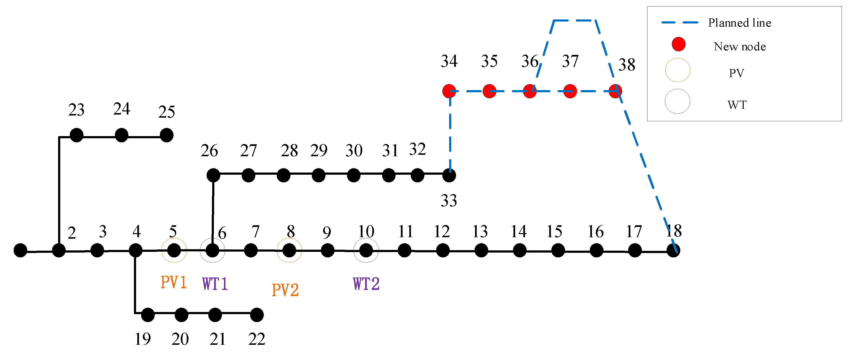
• Scenario 1: Add wind and solar power to the new 38-node distribution network.
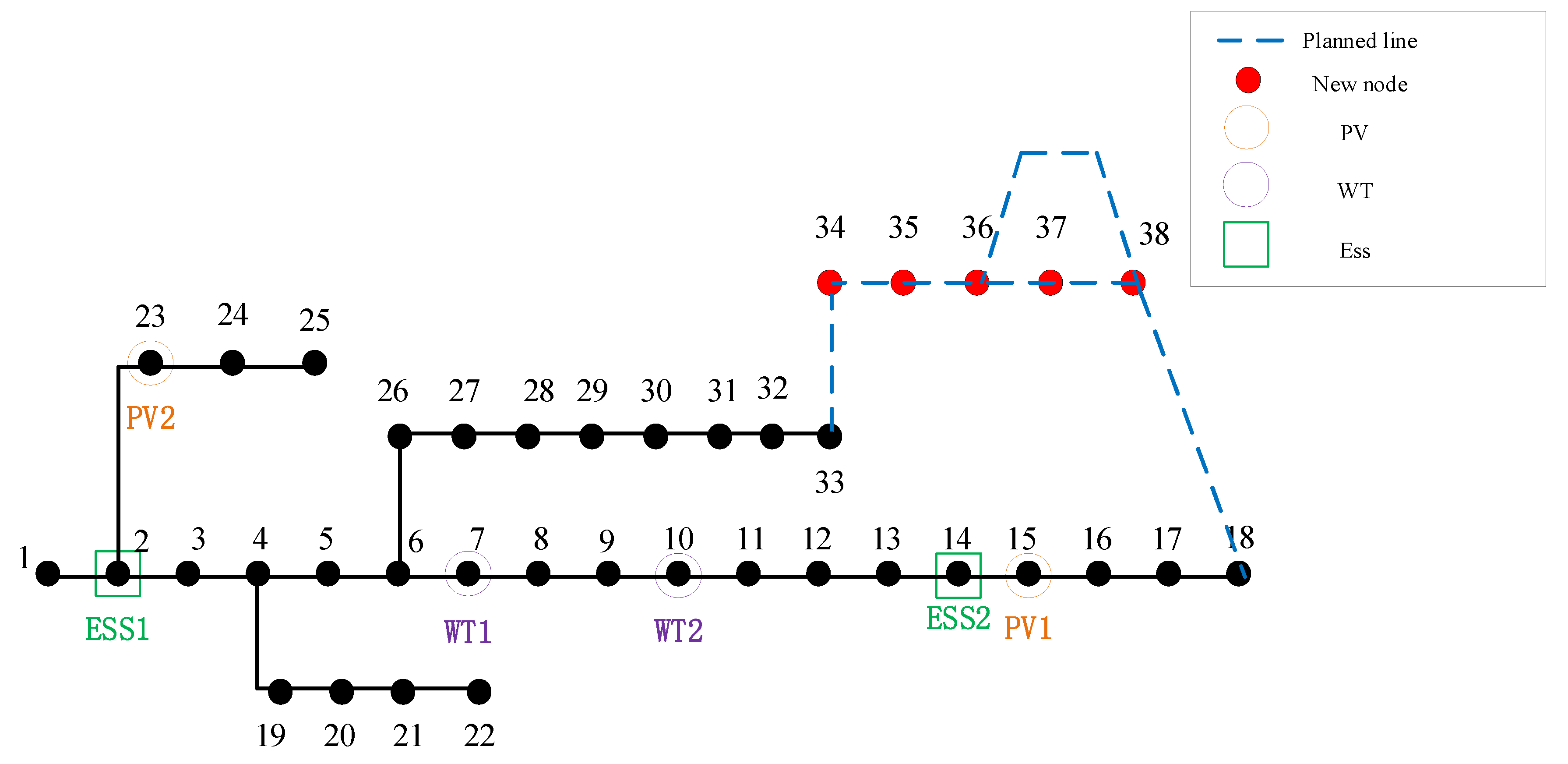
• Scenario 2: Add energy storage to Scenario 1.
• Scenario 3: On the basis of scenario 2, further reconfigure the new 38-node distribution network, incorporating the acceptance of wind, solar, and energy storage systems.

The results of the above scenarios are compared. Scenario 1 is compared with Scenario 2 to explore the impact of adding energy storage on the power supply capacity and renewable energy acceptance capacity of the distribution network. The results of Scenario 2 are then compared with Scenario 3 to investigate whether the reconstruction of the distribution network can improve the two capacities. All three scenarios use distributed generation equipment of the same specifications.

After calculations, the power supply capacity and renewable energy acceptance capacity for Scenario 1 and Scenario 2 are shown in Figure 4, while the impact of reconstruction on the power supply and renewable energy acceptance capacity of the distribution network is shown in Figure 5.

From the above Figure 4 and Figure 5, it can be observed that there is a clear positive correlation between the power supply capacity and the renewable energy acceptance capacity of distributed generation in the distribution network. In the early stages of distributed generation acceptance, as the renewable energy acceptance capacity increases, the power supply capacity rises rapidly. However, as the renewable energy acceptance capacity continues to grow, the increase in power supply capacity gradually stabilizes and eventually stops growing.

In Figure 4, Scenario 2 demonstrates a significant improvement in renewable energy acceptance capacity compared to Scenario 1. In Scenario 1, the power supply capacity of the distribution network stops increasing when the renewable energy acceptance capacity reaches approximately 0.35 MW. However, in Scenario 2, with the introduction of an energy storage system, the renewable energy acceptance capacity increases to approximately 0.6 MW. This indicates that the introduction of energy storage systems helps to improve the renewable energy acceptance capacity of the distribution network, enabling it to accept more distributed generation.

Nevertheless, while the addition of energy storage improves renewable energy acceptance capacity, its impact on power supply capacity is relatively limited. This is likely because energy storage primarily functions during load fluctuations and peak demand periods. Although it helps mitigate the uncertainty of distributed generation output, it does not directly increase the maximum power supply capacity of the distribution network. Once the renewable energy acceptance capacity reaches a certain threshold, the contribution of the energy storage system to both capabilities become saturated, and it can no longer effectively improve the system’s maximum power supply capacity, causing the overall curve to plateau.

Figure 5 compares Scenario 3 with Scenario 2. After reconfiguring the distribution network, the power supply capacity is further improved. When the renewable energy acceptance capacity reaches approximately 1.6 MW, the power supply capacity stabilizes. Compared to Scenario 2, Scenario 3 accepts approximately 0.9 MW more distributed generation, with a corresponding increase in power supply capacity of about 0.2 MW. From the growth curves of the two scenarios, Scenario 3’s curve is smoother than that of Scenario 2. This indicates that the reconfigured distribution network can further optimize the network structure, improving both the power supply capacity and renewable energy acceptance capacity of the system.

In summary, without considering uncertainty factors, the introduction of energy storage systems and the reconstruction of the distribution network have led to varying degrees of improvement in the power supply and renewable energy acceptance capacities. In Scenario 2, the introduction of the energy storage system significantly improves the renewable energy acceptance capacity of distributed generation, while the reconstruction strategy in Scenario 3 further optimizes the distribution network structure, improving the power supply capacity. This demonstrates that under the context of substantial distributed generation acceptance, the reasonable optimization of network structures and the application of energy storage systems play an important role in improving the power supply and renewable energy acceptance capacities of the distribution network.

5.2.2. Analysis of the Relationship Between Power Supply Capacity and Renewable Energy Acceptance Capacity Considering the Impact of Uncertainty

Based on the analysis of the results in the previous section, it can be observed that as the renewable energy acceptance capacity increases, the power supply capacity also increases, and then essentially ceases to grow. The relationship between the two satisfies the following equation:

$$P_{LSC}={\displaystyle \frac{a}{1+\exp (-b(P^{DG}-c))}}$$

(35)

where a, b, c are constants. $P_{LSC}$ represents the power supply capacity, and $P^{DG}$ represents the renewable energy acceptance capacity.

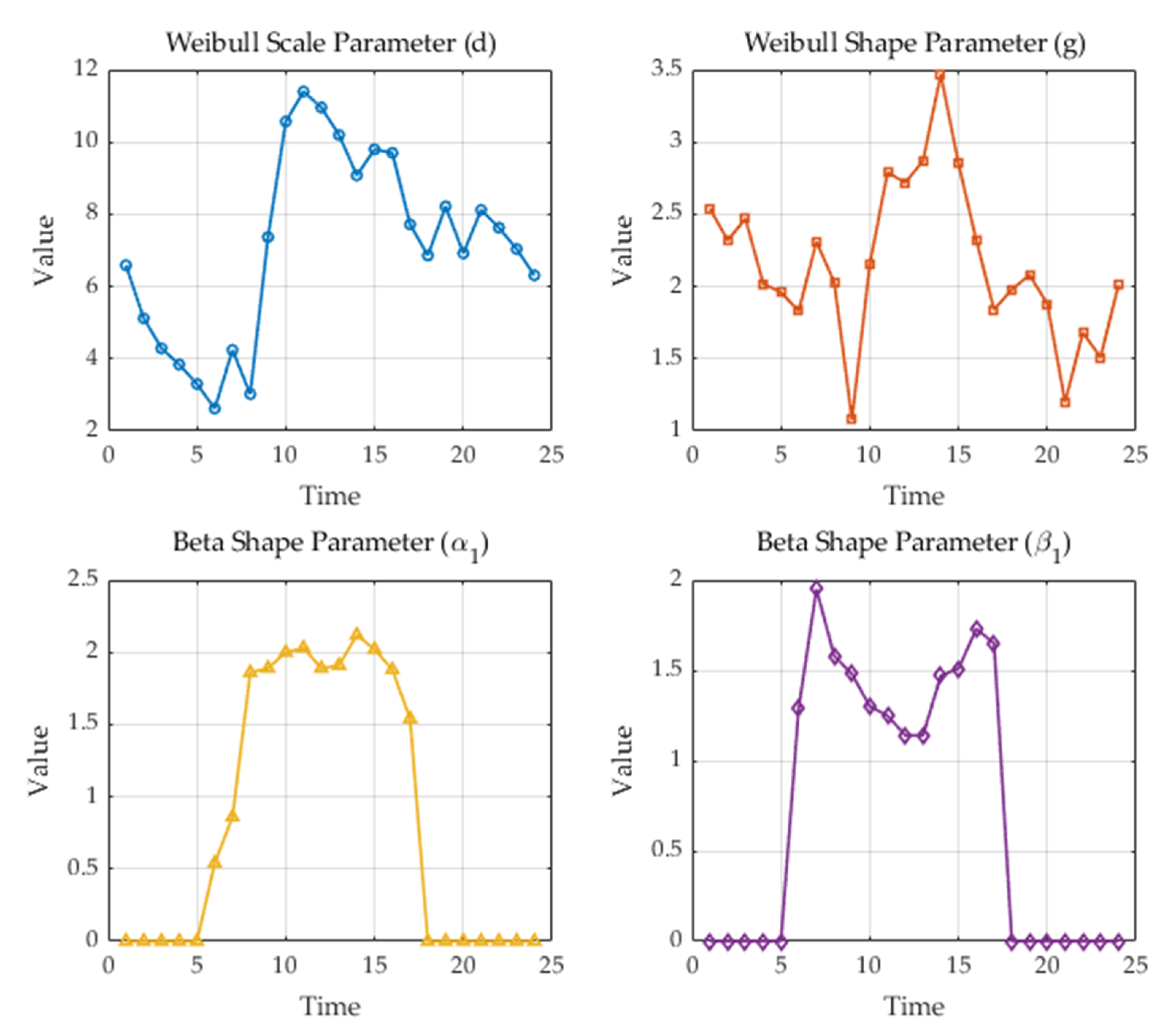
The impact of uncertainty on the distribution network is further considered based on the results of the previous section. Uncertainty factors are analyzed using Monte Carlo simulation with 5000 samples to minimize the influence of sample randomness. The parameters selected in this section are consistent with those in Section 5.1. The scenarios chosen for analysis are Scenario 2 and Scenario 3 from Section 5.2.1, with a confidence level of 0.85 for each constraint, to explore the impact of distribution network reconstruction under uncertainty. The planning costs for the two scenarios are shown in Section 5.2.3. The relationship between power supply capacity and renewable energy acceptance capacity under the two scenarios is illustrated in Figure 6 and Figure 7.

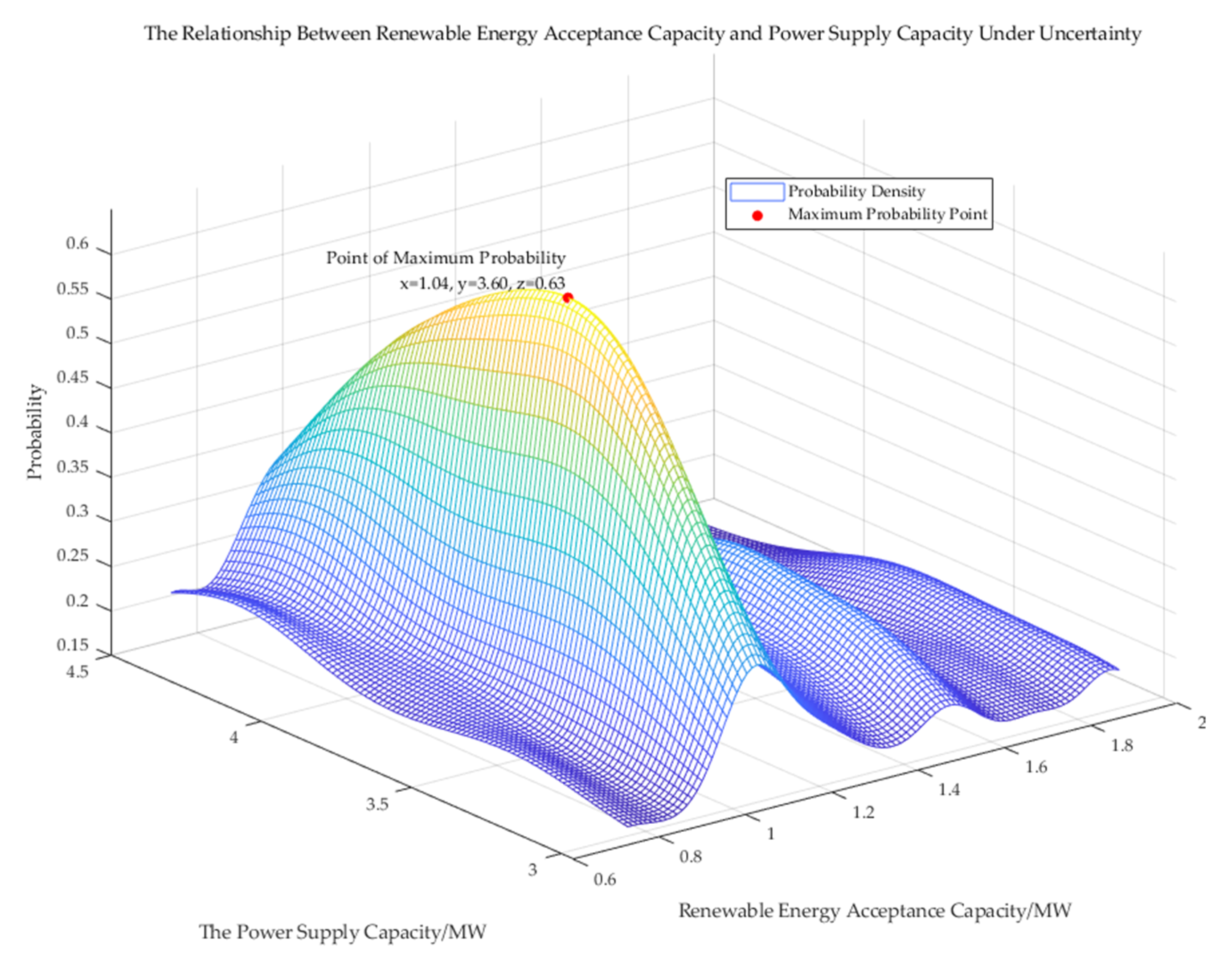
Through the comparative analysis of Figure 6 and Figure 7, it can be observed that under the confidence level of 0.85, the power supply capacity of the distribution network exhibits certain fluctuations. The relationship between the two capacities no longer shows a simple one-to-one correspondence but is instead presented in the form of a probability distribution. In this case, different renewable energy acceptance capacities correspond to different power supply capacities and associated probabilities.

In Figure 6, Scenario 2 before reconstruction shows a maximum probability of 0.63 when renewable energy acceptance is 1.04 MW and power supply is 3.60 MW. This indicates that under conditions of uncertainty, the distribution network in this scenario can operate relatively stably at this point. Although fluctuations exist, the position with the highest probability suggests optimal system stability under these conditions.

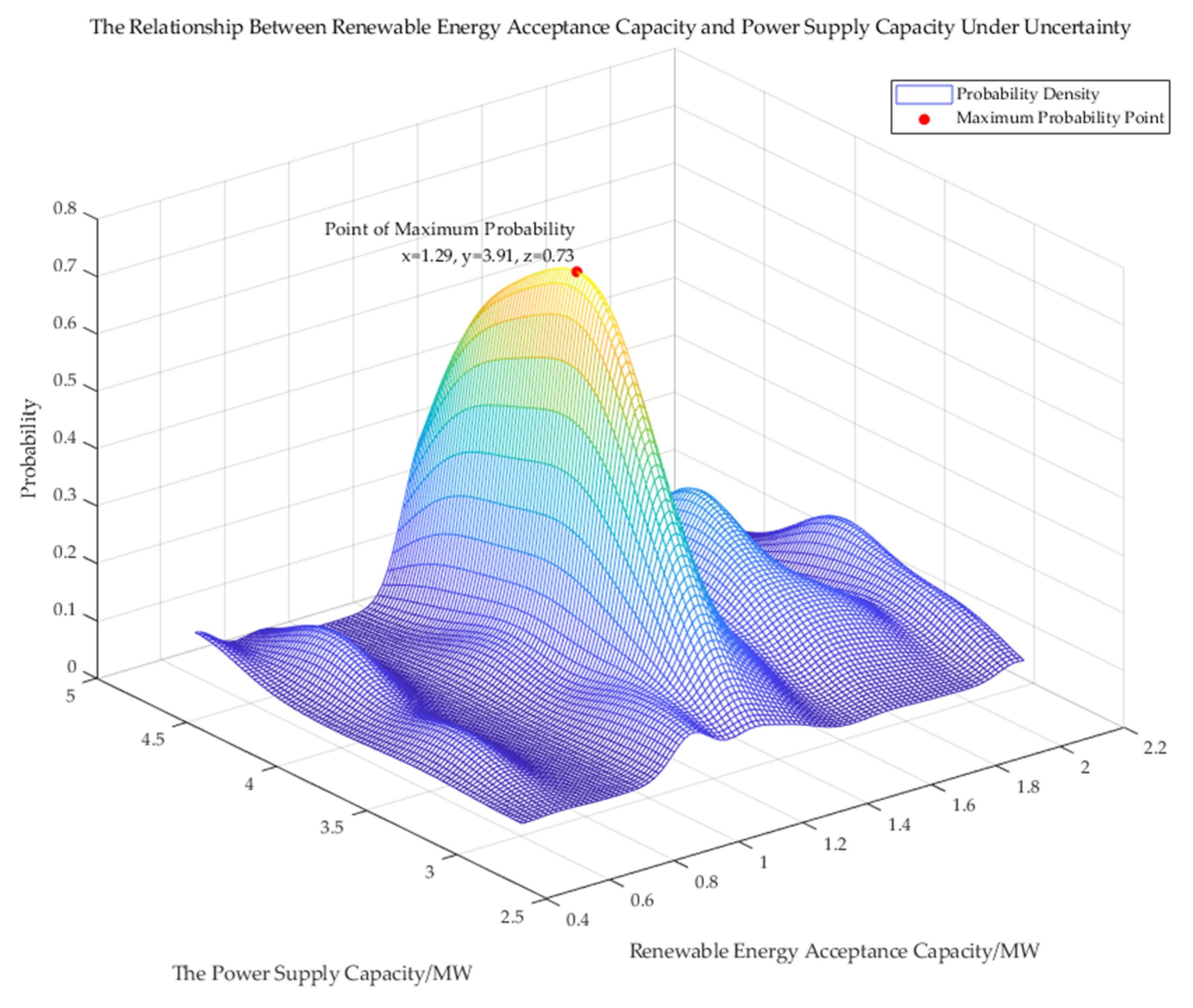
In Figure 7, after reconfiguring and optimizing the network structure, Scenario 3 demonstrates an increase in renewable energy acceptance capacity to 1.29 MW, with a corresponding increase in power supply capacity to 3.91 MW. The maximum probability at this point rises to 0.73. This not only shows that the reconfigured distribution network can accept more distributed generation but also reflects a simultaneous improvement in power supply and renewable energy acceptance capacities. The increased probability further validates the improved reliability of the optimized distribution network in addressing uncertainties.

However, both Figure 6 and Figure 7 reveal some non-peak probability points, which reflect significant fluctuations and lower occurrence probabilities for certain combinations of the two capacities at the current confidence level. These low-probability points may represent extreme operating states of the system, which should be avoided in practical planning to reduce potential threats to the safety and stability of the distribution network. Thus, resource allocation can be optimized to improve system operational efficiency and reliability.

5.2.3. Distribution Network Planning Results for the Three Scenarios

After calculations, the DG acceptance nodes for the three scenarios mentioned in Section 5.2.1 are shown in

Table 2. Distributed power planning access nodes for three scenarios.

Type	Scenario 1 DG Locations	Scenario 2 DG Locations	Scenario 3 DG Locations
Wind	6, 10	7, 10	4, 10
Photovoltaic	5, 8	15, 23	5, 15
Energy storage	-	2 (0.3), 14 (0.5)	2 (0.3), 18 (0.5)

(the data in parentheses indicate the renewable energy acceptance capacities in MW). The planning costs required for the three scenarios are shown in

Table 3. Investment planning results for the three scenarios.

Type	Scenario 1 Cost (10,000 CNY·year⁻1)	Scenario 2 Cost (10,000 CNY·year⁻1)	Scenario 3 Cost (10,000 CNY·year⁻1)
Energy storage investment cost, maintenance cost, network loss cost	20.45	24.32	23.67
Curtailment cost (wind/solar)	4.64	4.05	6.23
Outage cost	78.97	68.37	67.21
The network investment cost	55.13	55.13	54.54
Total cost	159.19	151.87	151.65

. The investment planning results for Scenarios 2 and 3 under uncertainty are shown in

Table 4. Investment planning results for Scenarios 2 and 3 under uncertainty.

Type	Scenario 2 Cost (10,000 CNY·year⁻1)	Scenario 3 Cost (10,000 CNY·year⁻1)
Energy storage investment cost, maintenance cost, network loss cost	29.67	28.54
Curtailment cost (wind/solar)	5.54	7.02
Outage cost	72.24	70.31
The network investment cost	55.13	54.54
Total cost	162.58	160.41

. The final planning results for Scenarios 1, 2, and 3 are illustrated in Figure 8, Figure 9, and Figure 10, respectively.

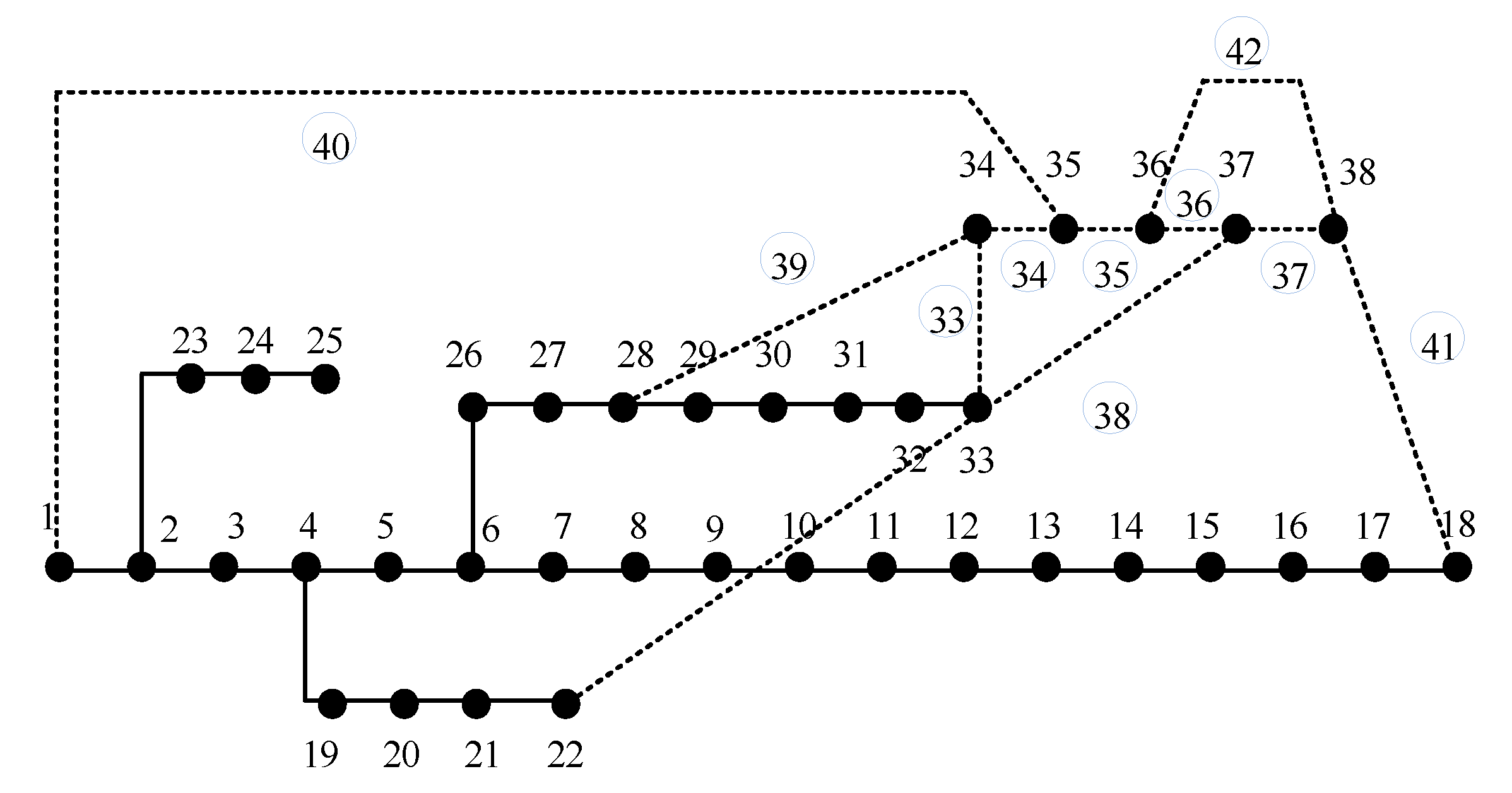
As shown in the figure, the new lines selected in Scenario 1 are lines 33–37, 41, and 42. The new lines selected in Scenario 2 are the same as those in Scenario 1. In Scenario 3, the selected lines are 33–37, 39, and 41.

From an economic perspective, the outage cost in Scenario 1 is approximately 100,000 CNY higher than in Scenario 2. However, the energy storage investment cost, maintenance cost, and network loss cost in Scenario 2 are about 40,000 CNY higher than in Scenario 1, which is likely due to the increased maintenance costs associated with adding energy storage. Despite this, the total cost of Scenario 2 is lower than that of Scenario 1, at 1.5187 million CNY and 1.5919 million CNY, respectively.

At the same time, energy storage can effectively reduce the amount of curtailed photovoltaic and wind energy, improve power quality, and improve supply reliability. Therefore, in terms of outage and curtailment costs, the economic performance of Scenario 2 is better than that of Scenario 1. Hence, under the same 38-node network structure, the scenario that includes energy storage is more suitable for the distribution network.

Through the comparative analysis of Table 3 and Table 4, it can be observed that the economic performance of Scenarios 2 and 3 shows significant differences under conditions with and without considering uncertainty factors. Firstly, the total cost of Scenario 2 is 1.5187 million CNY/year without considering uncertainty, but it rises to 1.6258 million CNY/year when uncertainty is taken into account, an increase of 107,100 CNY.

Among the cost components of Scenarios 2 and 3, the energy storage investment cost, maintenance cost, and network loss cost increase from 243,200 CNY/year to 296,700 CNY/year. This significant increase is mainly due to the intensified impact of distributed generation output uncertainty on system operations, leading to higher maintenance needs and network losses. In addition, the curtailment cost for wind and solar energy increases from 40,500 CNY/year to 55,400 CNY/year, indicating that the system struggles to fully utilize the surplus energy from distributed generation under uncertain conditions, resulting in greater resource waste.

The outage cost also rises, from 683,700 CNY/year to 722,400 CNY/year, further reflecting the negative impact of uncertainty on the system’s power supply stability.

In contrast, the total cost of Scenario 3 under conventional conditions is 1.5165 million CNY/year, and it rises to 1.6041 million CNY/year when considering uncertainty, an increase of 87,600 CNY, which is smaller than the increase in Scenario 2. This indicates that Scenario 3 has better economic adaptability when dealing with uncertainty.

The energy storage investment cost, maintenance cost, and network loss cost in Scenario 3 increase from 236,700 CNY/year to 285,400 CNY/year, a rise of 48,700 CNY. This increase is smaller than that of Scenario 2, demonstrating that the reconstruction strategy can more effectively handle the uncertainty brought by distributed generation. In addition, the curtailment cost for wind and solar energy in Scenario 3 rises slightly, from 62,300 CNY/year to 70,200 CNY/year, reflecting superior performance of the distribution network in terms of renewable energy acceptance capacity.

The outage cost increases from 672,100 CNY/year to 703,100 CNY/year, a rise of only 31,000 CNY, further proving the effectiveness of system reconstruction in improving power supply reliability.

Based on the results of this section and Section 4.2, the relationship curves of the two capacities in Scenario 3 (after reconstruction) and Scenario 2 (before reconstruction) show slight differences under varying conditions. The distribution network in Scenario 3 after reconstruction demonstrates significantly stronger power supply capacity and can accept a larger capacity of distributed generation.

However, economically, the reconfigured distribution network in Scenario 3 can integrate more distributed generation but may lead to higher costs for wind and solar curtailment, investment, maintenance, and network losses. This indicates that by sacrificing some economic performance, the reconfigured distribution network system can improve both the power supply capacity and the renewable energy acceptance capacity of the distribution network.

6. Conclusions

The study addresses the coupling relationship between power supply capacity and renewable energy acceptance capacity in distribution networks, focusing on the simultaneous improvement of both capacities. To achieve this, a network and energy storage joint planning and reconstruction strategy that accounts for source-load uncertainty is proposed. The main conclusions are as follows:

(1)

Quantitative Analysis of Coupling Relationship: A bi-level model was developed to quantify the relationship between power supply capacity and renewable energy acceptance capacity in distribution networks. The findings reveal that these capacities are positively correlated rather than independent, highlighting the interdependence necessitated by high levels of distributed generation (DG) integration.

(2)

Impact of Source-Load Uncertainty: Under conditions of source-load uncertainty, the previously observed direct correlation between power supply capacity and renewable energy acceptance capacity becomes more complex. The capacities exhibit fluctuations and are best represented through probability distributions, underscoring the need for robust planning approaches that can accommodate such variability.

(3)

Effectiveness of Joint Planning and Reconstruction Strategy: The proposed joint planning and reconstruction strategy effectively facilitates the optimal allocation of distributed generation and energy storage systems while reconfiguring the distribution network topology. This approach enables the simultaneous enhancement of power supply capacity and renewable energy acceptance capacity even under limited resource conditions, demonstrating its practical viability and efficiency.

(4)

Future Work and Suggestions: In future research, the inclusion of actual power market factors should be considered to provide more practical solutions for the sustainable development of distribution networks. Additionally, this study solely employed the PSO algorithm for the model’s computational aspect, which exhibits limitations in terms of solving efficiency. Therefore, adopting more advanced and complex solving algorithms in future work could enhance computational efficiency and overall model performance.

References

1. Wang, H.K.; Wang, S.X.; Pan, Z.X.; Wang, J.M. Optimized dispatching method for flexibility improvement of distribution network with high-penetration distributed generation. Autom. Electr. Power Syst. 2018, 42, 86–93. [Google Scholar]
2. Zhao, H.Z.; Chen, J.K.; Yang, H.Y.; Li, T.L.; Wang, H.K.; Wang, S.X. Expansion planning method of distribution network with distributed generation considering transmission capacity. Electr. Power Autom. Equip. 2021, 41, 70–77. [Google Scholar]
3. Wang, S.; Dong, Y.; Wu, L.; Yan, B. Interval overvoltage risk based PV hosting capacity evaluation considering PV and load uncertainties. IEEE Trans. Smart Grid 2019, 11, 2709–2721. [Google Scholar] [CrossRef]
4. Zhang, J.K.; Wei, G.; Zhu, L.; Chi, J.Y. Blind-number model based power supply capability evaluation of distribution networks with distributed generators. Autom. Electr. Power Syst. 2016, 40, 64–70. [Google Scholar]
5. Zhang, J.A.; Gao, X.D.; Wang, T.C.; Li, Z.J.; Deng, X.Y. Evaluate the hosting capacity of PV in distribution network considering PV curtailment constraints. Electr. Power Eng. Technol. 2023, 42, 14–21. [Google Scholar]
6. Dai, Q.; Li, J.; Hu, G.Y.; Zheng, B.L.; Li, J. Calculation of power supply capacity of distribution network with stochastic chance constraints considering wind power randomness. Hubei Electr. Power 2017, 41, 11–17. [Google Scholar]
7. Yang, G.; Guan, L.; Lin, L.X.; Yu, L.; Chen, H.A. Analysis of influences of grid-connected distributed generation on feeder power supply ability in distribution network. Proc. CSU-EPSA 2020, 32, 13–20. [Google Scholar]
8. Wang, X.Q.; Wang, L.Y.; Zhang, G.; Zhou, X.C.; Zhang, H. Impact analysis of DG access on feeder power supply capability in distribution network. China Acad. J. Electron. Publ. House 2021, 21, 47–49. [Google Scholar]
9. Abad, M.S.S.; Ma, J. Photovoltaic hosting capacity sensitivity to active distribution network management. IEEE Trans. Power Syst. 2021, 36, 107–117. [Google Scholar] [CrossRef]
10. Chihota, J.M.; Bekker, B.; Gaunt, T. A stochastic analytic-probabilistic approach to distributed generation hosting capacity evaluation of active feeders. Int. J. Electr. Power Energy Syst. 2022, 136, 107598. [Google Scholar] [CrossRef]
11. Wu, H.; Sun, L.W.; Xiang, S.; Yuan, Y. Expansion planning of active distribution network considering high-dimensional temporal correlation between renewable energy and load. Autom. Electr. Power Syst. 2022, 46, 40–51. [Google Scholar]
12. Wu, Y.; Liu, H.T.; Xiao, Z.F.; Chen, Z.W.; Liu, P.; Hou, H.; Tang, A.H.; Cui, R.J. Review of incremental distribution network planning considering the uncertainty of source-network load. Power Syst. Prot. Control 2021, 49, 177–187. [Google Scholar]
13. Ge, S.Y.; Zhang, Y.W.; Liu, H.; Li, T. Bi-layer expansion programming method for active distribution network considering dynamic grid reconstruction. Power Syst. Technol. 2018, 42, 1526–1536. [Google Scholar]
14. Wang, C.S.; Chen, K.; Xie, Y.H.; Xie, H.F. Siting and sizing of distributed generation in distribution network expansion planning. Autom. Electr. Power Syst. 2006, 8, 38–43. [Google Scholar]
15. Yang, X.Y.; Mu, G.; Chai, G.F.; Yan, G.; An, J. Source-storage-grid integrated planning considering flexible supply-demand balance. Power Syst. Technol. 2020, 44, 3238–3246. [Google Scholar]
16. Xu, W.; Yang, Y.Q.; Zhang, L.; Xia, Y.; Li, K. A dual-layer planning strategy for distribution network based on source-load temporal characteristics. Trans. Chin. Soc. Electr. Power Syst. Autom. 2024, 37, 17–25. [Google Scholar]
17. Cai, J.M.; Zhang, T.; Wang, C.M.; Xie, N.; Zhu, B. Flexible planning of active distribution network expansion considering source and load uncertainty. Electr. Power Autom. Equip. 2019, 39, 109–115. [Google Scholar]
18. Yi, H.C.; Zhang, P.D.; Wang, H.Y.; Wu, Y.; Yuan, G.S.; Lv, R.R. Distribution network dynamic reconstruction method for improving distribution network’s ability of accepting DG. Power Syst. Technol. 2016, 40, 1431–1436. [Google Scholar]
19. Jin, Y.Z.; Zhang, L.P.; Niu, Q.F. Reconfiguration of distribution network with wind power generators considering randomness and fuzziness. Proc. CSU-EPSA 2020, 32, 67–72. [Google Scholar]
20. Long, Y.; Wang, X.Y.; Zhou, Q.; An, H.Y.; Chen, Z. Distribution network reconfiguration for loss reduction considering maximum power supply capability index. Proc. CSU-EPSA 2017, 29, 131–134. [Google Scholar]
21. Zhu, J.P.; Gu, W.; Zhang, H.D.; Wang, W.J.; Zhu, G.; You, D.J. Optimal siting and sizing of distributed generators considering dynamic network reconfiguration. Autom. Electr. Power Syst. 2018, 42, 111–119. [Google Scholar]
22. Luo, T.; Zhao, G.S.; Yan, D.W.; Zhang, Z. A probabilistic assessment method for distribution network’s distributed PV hosting capacity considering the feeder reconstruction. Proc. CSU-EPSA 2024, 1, 1–11. [Google Scholar]
23. Li, P.R. Active Distribution Network Power Supply Capacity Assessment Taking into Account Wind-Scenery Uncertainty. Master’s Thesis, Guizhou University, Guiyang, China, 2021. [Google Scholar]
24. Shi, R.J.; Wang, W.Q.; Fan, X.Z.; Wang, J.L.; Zhang, W.W. Analysis of energy storage operation and configuration in high proportion wind power systems. Water Power 2024, 1, 1–9. [Google Scholar]
Figure 1. Logical diagram of the network and energy storage joint planning and reconstruction strategy model.
Sustainability 17 01292 g001
Figure 2. Flowchart for solving the bilayer model.
Sustainability 17 01292 g002
Figure 3. Topology of the proposed 38-node distribution network.
Sustainability 17 01292 g003
Figure 4. Relationship between the power supply capacity and the renewable energy acceptance capacity of the distribution networks of Scenario 1 and Scenario 2.
Sustainability 17 01292 g004
Figure 5. Relationship between the power supply capacity and the renewable energy acceptance capacity of the distribution networks of Scenario 2 and Scenario 3.
Sustainability 17 01292 g005
Figure 6. Exploration of the relationship between power supply capacity and renewable energy acceptance capacity before reconstruction.
Sustainability 17 01292 g006
Figure 7. Exploration of the relationship between power supply capacity and renewable energy acceptance capacity after reconstruction.
Sustainability 17 01292 g007
Figure 8. Final plan for Scenario 1.
Sustainability 17 01292 g008
Figure 9. Final plan for Scenario 2.
Sustainability 17 01292 g009
Figure 10. Final plan for Scenario 3.
Sustainability 17 01292 g010