The Role of Solar Gains in Net-Zero Energy Buildings: Evaluating and Optimising the Design of Shading Elements as Passive Cooling Strategies in Single-Family Buildings in Colombia

Abstract

Net zero-energy buildings have become one of the flagships in the path towards the decarbonisation of cities. Even though heating systems, especially in existing buildings, are currently the main consumer in many areas of the world, cooling needs are gaining relevance in several countries, and this is expected to be kept in the focus in the context of increasing temperatures, according to the climate projections identified by the IPCC. This has also additional implications on thermal comfort conditions (and, indirectly, on the derived health issues) in areas where no cooling systems are installed in residential buildings. This research work aims to evaluate the design of shading elements as a design strategy in the path towards net-zero residential buildings in diverse Colombian climates. A parametric analysis is developed, considering a combination of different shading solutions applied in residential buildings. Their effectiveness is evaluated in different climate zones in Colombia considering both the current climate data and future climate data expected according to the projections proposed by the IPCC. A reference building in Bucaramanga (Colombia) was selected for detailed monitoring, and the collected data were used to validate a simulation model developed in DesignBuilder. Almost 1000 alternative scenarios were established and parametrically evaluated, resulting from the combination of different shadings solutions, orientations and climate conditions. The results are evaluated considering two different approaches: cooling demand assuming a standard indoor temperature profile and indoor comfort when no cooling devices are used in the building, showing that some strategies, such as overhangs, involve significant improvements in terms of indoor thermal comfort and a reduction in cooling demand (reaching in some cases savings up to 30%) in the different climate conditions considered; as well, their effectiveness remains similar when future climate projections are considered.

1. Introduction

The building sector, responsible for approximately 38% of global carbon emissions, plays a crucial role in addressing climate change. Net-Zero Energy Buildings (NZEBs) and Net-Zero Carbon Buildings (NZCBs) have emerged as essential strategies for reducing operational and embodied carbon. These concepts aim to decarbonise the sector by integrating passive design solutions and renewable energy systems. Despite advancements, implementing these measures in equatorial regions remains underexplored. The specific climatic conditions, with consistently high solar radiation and temperatures, provide both opportunities and challenges for passive cooling strategies, particularly shading design, as a means to reduce energy demand and improve thermal comfort [1,2].

1.1. NZEBs in Tropical and Equatorial Areas

The global transition towards decarbonisation has underscored the need for sustainable building practices, particularly through the adoption of Net-Zero Energy Buildings (NZEBs). These structures, designed to balance energy consumption and production, have been extensively researched in temperate and cold climates, where heating needs dominate energy demands [3,4]. However, even though there has been extensive scientific activity regarding NZEBs in general, research works focused on NZEBs in tropical and equatorial climates are limited. Moreover, such strategies are critical for aligning with global decarbonisation goals and preparing for the rising energy demands anticipated due to climate change. Projections indicate a significant increase in cooling energy requirements globally, particularly in warmer climates, as urbanisation and rising temperatures exacerbate indoor heat stress [3,5]. In this regard, considering not only energy demand but also thermal comfort is a critical challenge in the design of effective passive cooling strategies. In recent decades, the development of several simulation tools has allowed to perform a precise evaluation of shading designs and their impacts, providing a robust framework for passive cooling optimisation [6].

In tropical and equatorial regions, where high solar exposure persists throughout the year, shading solutions play a critical role in minimising cooling energy demand. Passive cooling strategies, particularly shading, are identified as effective means to reduce cooling loads in buildings, particularly in regions with high solar radiation. Previous studies show that shading solutions can significantly mitigate solar heat gains while enhancing indoor thermal comfort [7]. A research piece conducted in Southeast Asia and South America highlights the potential of shading elements to reduce cooling loads by up to 30%, depending on the building’s orientation and the type of shading employed [8]. Furthermore, combining shading with other passive strategies, such as natural ventilation and reflective materials, enhances overall building performance, particularly in hot and humid climates [9]. Similar conclusions can be extracted from the work presented by Al-Masrani et al. in [10], focused on Malaysia and Singapore, a work where the efficiency of different shading systems (such as overhangs and vertical fins) in the tropics is emphasised. Meanwhile, adjustable or dynamic shading solutions, such as louvers and automated blinds, offer greater adaptability to changing solar angles and varying climatic conditions, further optimising indoor environments [11].

Finally, the importance of approaching this issue not only from the energy demand perspective but also considering indoor thermal comfort conditions should be noted. While energy demand quantifies the energy required to maintain acceptable indoor conditions, thermal comfort reflects subjective occupant experiences. In this regard, shading solutions tailored to specific orientations and solar exposures can optimise both parameters, improving occupant satisfaction while reducing energy consumption [12].

These findings are particularly relevant in Colombia, where climatic diversity—from humid coasts to cooler highlands—offers a rich context for evaluating the adaptability of different shading designs. Furthermore, Colombia’s recent national roadmap for reducing greenhouse gas emissions in buildings aligns with the objectives of this study, emphasizing the potential for passive measures to contribute to national and global sustainability goals. Additionally, it is expected that in the context of climate change, this will become even more urgent in the next decades. Projections from the IPCC (Intergovernmental Panel on Climate Change) and other climate models underline the increasing relevance of cooling demand as global temperatures rise. In regions near the equator, these trends are anticipated to exacerbate energy use in buildings, emphasising the importance of integrating adaptive measures like shading into building design [3,13]. Research further supports the role of localised climate-specific solutions, which are shown to be more effective than generalised design approaches [14].

Thus, the work presented in this paper builds on these findings, focusing on the adaptation and optimisation of shading strategies for Colombia’s diverse climate zones. Additionally, integrating IPCC climate projections, this research work also highlights the urgency of implementing adaptive shading strategies to mitigate the impact of increasing global temperatures [15]. By leveraging advanced simulation tools and considering both current and future climate scenarios, it aims to provide actionable insights into the integration of shading solutions as a cornerstone of sustainable residential design. Additionally, the analysis presented in this work takes into consideration both cooling demand and thermal comfort.

In that sense, this paper makes a significant contribution to the field of sustainable building design by addressing a critical gap in the literature: the optimisation of shading strategies for equatorial climates, specifically in Colombia. While extensive research has focused on passive cooling in temperate and tropical regions, studies tailored to the unique climatic conditions of latitudes near the equator remain scarce. This geographic bias underscores the novelty of evaluating shading strategies in Colombian climates, characterised by year-round cooling needs due to stable temperatures. By conducting a detailed analysis of shading solutions across Colombia’s diverse climate zones, this research not only advances the understanding of passive cooling strategies but also provides a replicable framework for similar regions globally. The integration of both current and projected climate scenarios further underscores the relevance of this work in the context of climate change, highlighting its potential to inform future policy and design practices aimed at reducing energy consumption and improving thermal comfort in residential buildings.

1.2. Objectives and Research Questions

Hence, the main objective of this paper is to optimise the designs of several shading and solar gain management strategies as well as evaluate their impacts on the thermal performance of residential buildings from the point of view of thermal comfort and cooling demand, considering the different climates existing in Colombia. It should be noted that this work focuses on fixed elements; movable elements are out of the scope of this study.

To do this, a set of secondary objectives are identified:

• Firstly, a representative residential building is selected, and a monitoring study is carried out, with the aim of obtaining relevant data regarding its indoor thermal conditions.
• Secondly, a building simulation model is defined, validated and calibrated with the data obtained from the monitoring study.
• Finally, the model is used to design and evaluate a set of different strategies with the aim of evaluating their impact, considering both the cooling demand and indoor comfort, not only assuming different orientations and locations (representative of the different Colombian climates) but also considering one of the future climate scenarios projected by the IPCC. Thus, 960 different combinations were simulated under two different approaches (resulting, then, in 1920 simulations), and the obtained results were carefully analysed. Additionally, these results are publicly available in a data set stored in Mendeley Data Repository [16].

These objectives, in turn, have given rise to the three research questions that this paper aims to address:

• RQ1. What is the optimal design of different shading solutions for latitudes close to the equator?
• RQ2. What impacts do orientation and location have on the design of these strategies?
• RQ3. What impact do these measures have in terms of cooling demand reduction and thermal comfort?

By addressing these aspects, as previously mentioned, this research builds on a growing body of literature, extending the understanding of NZEB strategies to equatorial regions, with a specific focus on Colombia’s climatic diversity. The findings aim to contribute to the global discourse on sustainable building practices and offer a reference for future studies in similar latitudes.

With the aim of meeting these objectives and answering the research questions raised, the rest of the paper is organised as follows: The method followed in this research work is detailed in Section 2 and Section 3. Section 2 describes the general procedure followed to reach the aforementioned objectives, from the selection and description of the residential building used as a case study and the monitoring study carried out in it, whereas the model definition, model validation and the design of the simulations carried out, as well as the considered combinations, are detailed in Section 3. The section finishes with a brief description of the criteria and method followed to analyse the obtained results. In Section 4, the results obtaining are analysed and discussed, considering two different approaches, as described later in detail: one focused on the cooling demand and the other one focused on analysing the impacts on indoor thermal comfort. The main conclusions of this research piece are summarised in Section 5.

2. Materials and Methods

To carry out this research work, the process is organised into six main stages. Firstly, (i) a detailed analysis of the residential building stock in Bucaramanga is carried out, and a representative residential building (a single-family building) is selected to use as a case study in this work; (ii) the building is monitored for one month, with the aim of obtaining detailed data of the indoor thermal conditions; (iii) a detailed model of the reference building is defined in Design Builder, and it is calibrated and validated using the data obtained in the monitoring study; (iv) a set of strategies for reducing cooling demand are identified, as well as some of the main parameters to be defined; (v) a package of 960 scenarios resulting from the combination of these parameters with different orientations and different Colombian locations (Bucaramanga, Cali, Barranquilla, Medellín and Bogotá) is simulated, considering not only present climate data but also expected climate data in the future based on IPCC projections; finally, (vi) the sixth stage involves the analysis of the results obtained, considering two different approaches: their impacts on indoor thermal comfort and the impact on the cooling demand.

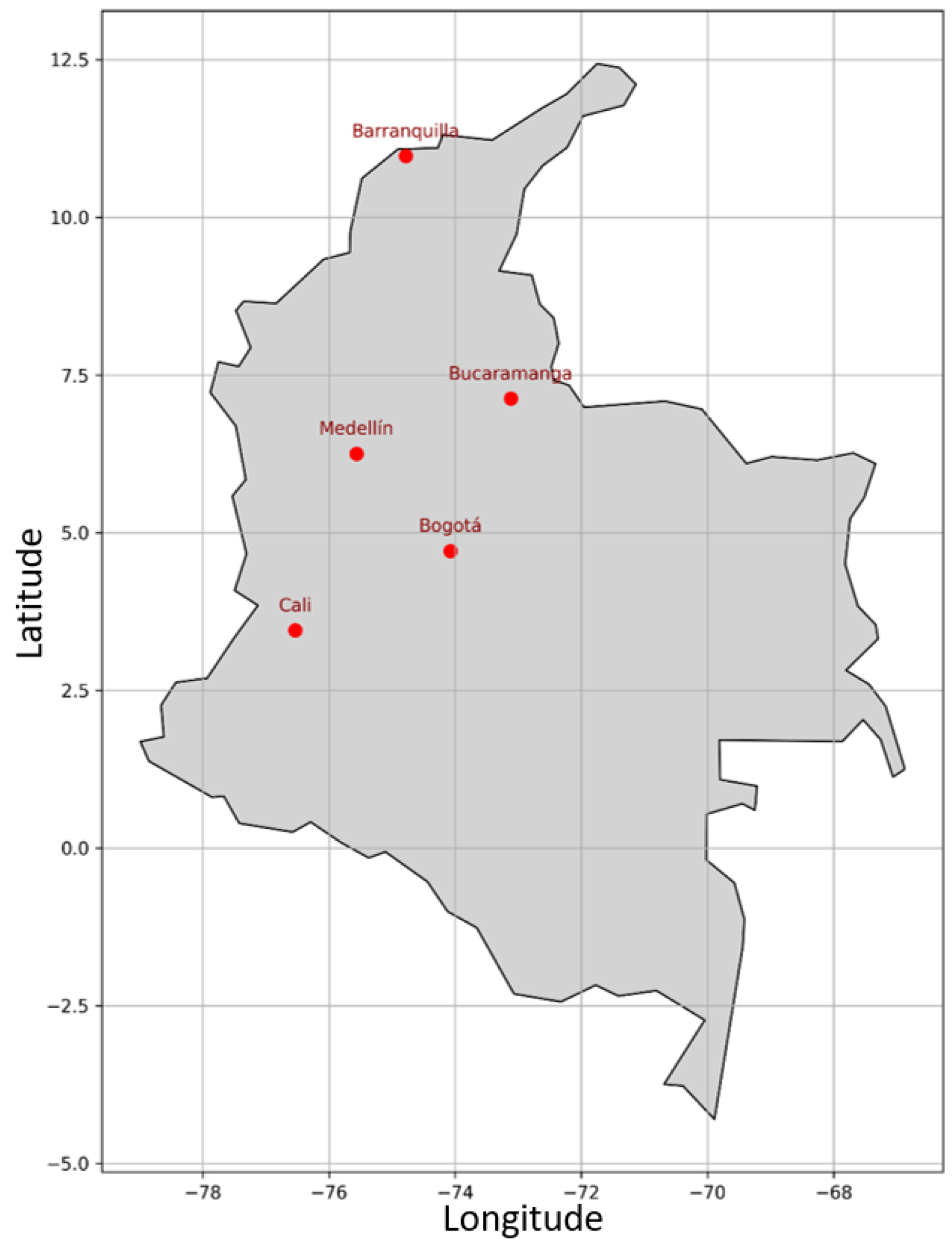
2.1. Case Study: A Terraced House in Bucaramanga, Colombia

The case study selected is considered a representative case of single-family dwellings in the study area. The building, located in Bucaramanga (Santander, Colombia), is a two-storey terraced house built in 1990, east–west oriented, with a total area of 126 m² distributed over two floors. As far as the construction features are concerned, it has an envelope of 0.12 m thick brick sheeting clad on both sides with a 0.025 m thick layer of plastic cement. Internal partitions are made of 0.12 m bricks with a coating on both sides of plastic cement. The floor is made up of 0.07 m cast concrete (outer part), 0.02 m plastic cement and 0.02 m ceramic tiles (inner part). The roof is made of clay tiles fixed to concrete. The windows have a single pane of 3 mm glass and an aluminium frame. As many others in the region, this house does not have an active heating or cooling system.

2.2. Monitoring Study

With the aim of obtaining data for validating and adjusting the building model, the building was monitored. The monitoring study was carried out for 30 days in the spring of 2020, between the 1st and 31st of May, by collecting temperature and relative humidity data. This period was selected based on the expected cooling demands: even though this area presents a cooling demand profile that is quite similar over the whole year, it generally trends to be slightly higher in the period from May to September. The building was occupied, and it kept the usual operation profiles during the monitoring period. A detailed description about this study is provided in the text below.

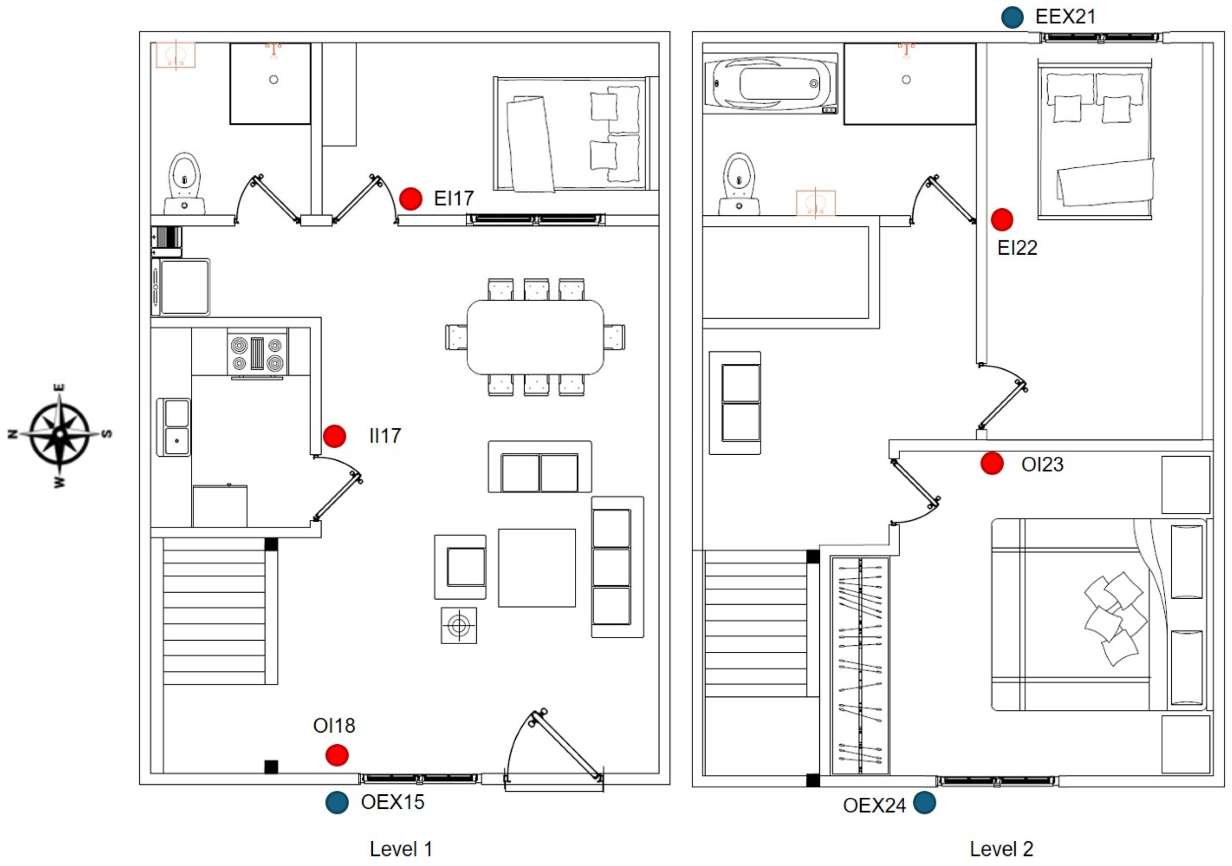
2.2.1. Monitoring Equipment and Sensor Placement

The monitoring system utilised WS-3000 sensors, provided by Ambient Weather (Chandler, AZ, USA), configured to record hygrothermal conditions within the building. These sensors collected temperature and relative humidity data at three-minute intervals. The technical specifications of the WS-3000 sensors include a temperature measurement range from −40 °C to 60 °C with a resolution of 0.1 °C and relative humidity measurement between 10% and 99% with an accuracy of ±5% for the 20–90% range. A detailed summary of the sensor specifications is provided in

Table 1. Specifications of the WS-3000 sensors used for monitoring.

Measure	Range	Error	Resolution
Indoor temperature	−40–60 [°C]	+0.1 [°C]	0.1 [°C]
Outdoor temperature	−40–60 [°C]	+0.1 [°C]	0.1 [°C]
Indoor humidity	10–99%	+5%	1%
Outdoor humidity	10–99%	+5%	1%

.

The locations of the sensors were carefully planned to reflect the thermal conditions across different zones of the building.

Table 2. Sensor coding and locations.

Channel	Code	Location
Channel 1	(EEX21)	East zone, external wall, upper floor
Channel 2	(EI22)	East zone, internal wall, upper floor
Channel 3	(OI23)	West zone, internal wall, upper floor
Channel 4	(OEX24)	West zone, external wall, upper floor
Channel 5	(EEX15)	East zone, external wall, ground floor
Channel 6	(EI16)	East zone, internal wall, ground floor
Channel 7	(II17)	Central zone (intermediate area of the house)
Channel 8	(OI18)	West zone, internal wall, ground floor

provides the coding and location of each sensor, while Figure 1 illustrates their strategic distribution.

Figure 1 illustrates the strategic positioning of sensors both inside and outside the building. The zones are categorised based on their orientation and function: east-facing, west-facing, and central areas. This layout ensures comprehensive monitoring of temperature and humidity variations influenced by solar exposure and building geometry. It also highlights the differentiation between upper and lower floors to account for vertical thermal stratification.

• Outdoor sensors: Three sensors were installed to monitor environmental conditions. Two were located on the eastern façade to capture morning solar gains, with one on the western façade to measure the effects of afternoon solar exposure.
• Indoor sensors: Five sensors were positioned within the building. One was on the ground floor, one sensor was placed in an east-facing room to record morning thermal gains, one was in a west-facing room to monitor afternoon heat effects, and another was in a centrally located room to establish baseline conditions. On the upper floor, one sensor was located in an east-facing bedroom and another in a west-facing bedroom to capture vertical stratification and room-specific dynamics.

2.2.2. Monitoring Campaign

As previously mentioned, the monitoring campaign was conducted over 30 consecutive days. Data were recorded at three-minute intervals, resulting in a high-resolution data set that captured both diurnal and nocturnal variations in temperature and humidity. This approach ensured a detailed analysis of the dynamic hygrothermal conditions within the building.

The monitoring study coincided with the COVID-19 pandemic, which led to continuous occupancy of the house. The prolonged presence of the occupants (2 people) influenced heat loads and ventilation patterns (on a general basis, windows were open during the night-time), providing valuable insights into the interaction between human activities and the performance of passive cooling strategies.

Complementary data on external weather conditions, such as solar radiation intensity, ambient temperature and wind speed, were obtained from a nearby meteorological station and provided by the Institute of Hydrology, Meteorology and Environmental Affairs (IDEAM, Instituto de Hidrología, Meteorología y Asuntos Ambientales), a Colombian governmental agency [17]. Namely, the data correspond to the weather station located in the Palonegro International Airport of Bucaramanga, located 13 km away from the case study building. Data were provided on an hourly basis. These external parameters were critical for contextualising the indoor measurements and understanding the external thermal drivers affecting the building.

2.2.3. Measurement Parameters and Spatial Configuration

The study focused on two primary variables: temperature and relative humidity, measured both indoors and outdoors. Relative humidity was monitored due to its significant impact on occupant comfort. To analyse the spatial dynamics, the building was divided into three zones based on the locations of the sensors:

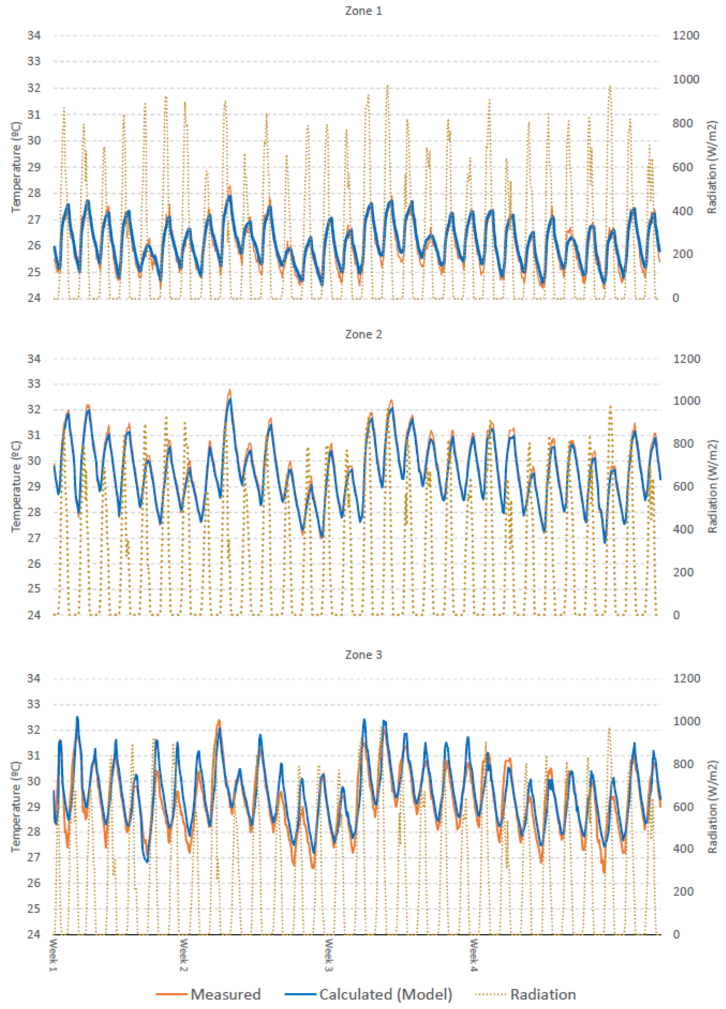
• Zone 1: the entire ground floor, including east-facing, west-facing, and central rooms (even though three sensors were placed on the ground floor (two in the living room and one in the bedroom), the measured temperature profiles were quite similar, and only one zone was considered to make the analysis clearer, assuming a profile obtained from the average values measured by the three sensors);
• Zone 2: east-facing rooms on the upper floor;
• Zone 3: west-facing rooms on the upper floor.

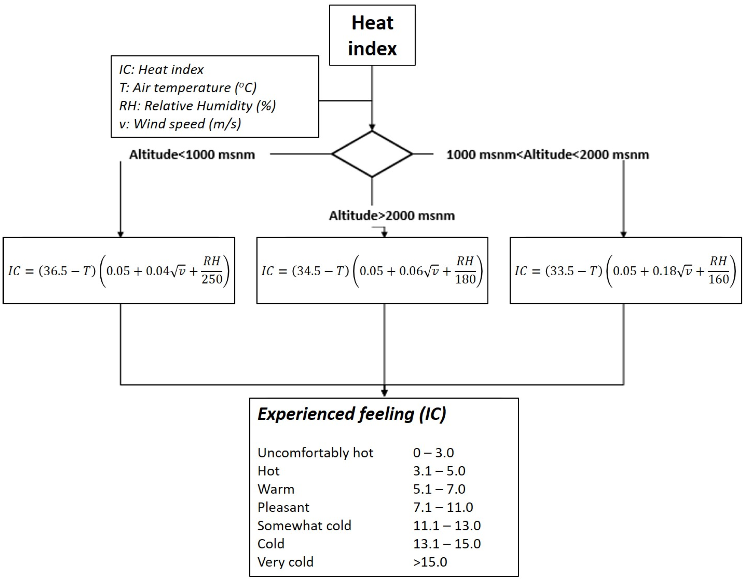
2.2.4. Analysis Framework

The collected data were processed to investigate the temporal and spatial thermal dynamics, with a focus on solar heat gains and thermal comfort. Solar gains were assessed by analysing the effect of direct radiation on indoor temperatures, particularly in east- and west-facing rooms. This analysis highlighted the impact of solar orientation on temperature fluctuations.

Thermal comfort was evaluated using indices such as the Cooling Power Index and other adaptations for tropical climates that are later detailed in Section 3.6, incorporating both temperature and humidity data. This allowed for a detailed assessment of how the indoor environment influenced occupant comfort and well-being over time.

3. Building Modelling and Definition of Scenarios

A model of the reference building was developed using Design Builder software (v. 7.3) [18], enabling the analysis of thermal performance, including indoor conditions and annual cooling demands. This software is a graphical user interface for the EnergyPlus solver [19], whose suitability for building energy evaluations has been demonstrated in several academic works for different purposes [20,21,22]. Additionally, this tool was also selected due to its potential to automatise large sets of simulations, as shown in other previous works (e.g., [23]).

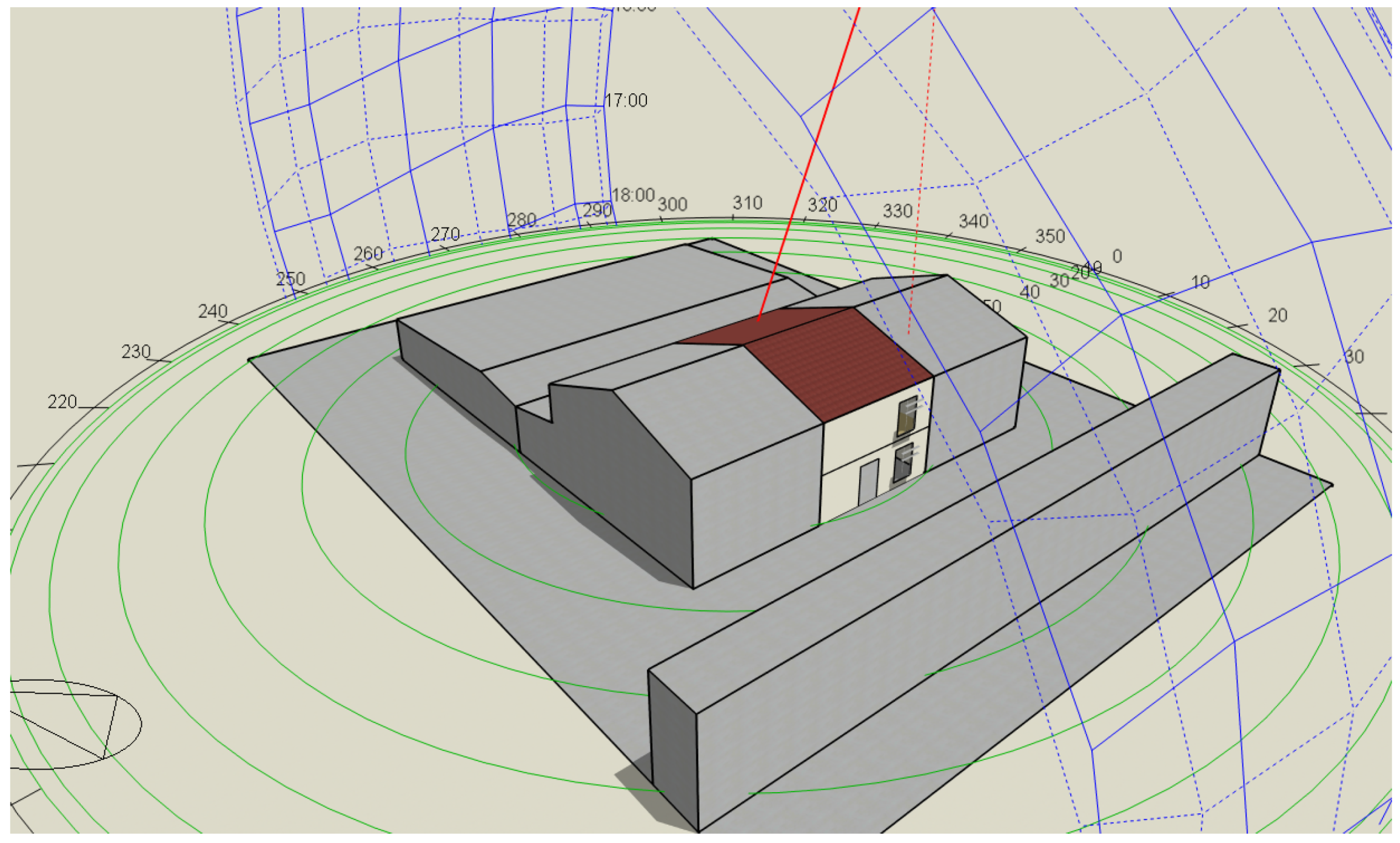
3.1. Model Definition

Nine different thermal zones were assumed for defining the model based on the internal distribution presented in Figure 1: five on the ground floor (living room, bedroom, bathroom, kitchen and stairs) and four on the upper floor (two bedrooms, bathroom and stairs). As far as thermal characterisation is concerned, it is defined on the basis of the construction characteristics of the case study, which were already described in Section 2.1. Thus, a U-value of 2.32 W/m²·K was assumed for façade walls and single glazing panes with an aluminium frame (with no thermal break), with a resultant U-value of 5.8 W/m²·K assumed in the case of windows. Additionally, the internal partitions between the case study dwelling and the adjacent buildings were assumed as adiabatic walls, since, for the purposes of this study, it could be assumed that the use profiles in adjacent dwellings would be quite similar and, as a consequence, with similar indoor thermal conditions. This assumption is normal, and it has been assumed in previous studies, such as [24]. Regarding internal gains, an hourly basis profile was assumed based on the use of the building during this period (two people living in the dwelling), considering 2 W/m² during the night-time (from 11 pm to 6 am) and a baseline of 4 W/m² for the daytime (from 6 am to 11 pm), with a peak consumption of 10 W/m² in the evening, namely from 6 pm to 10 pm. The same criteria were assumed for ventilation, assuming a windows were open during the night-time. A general view of the geometry of the building model is presented in Figure 2.

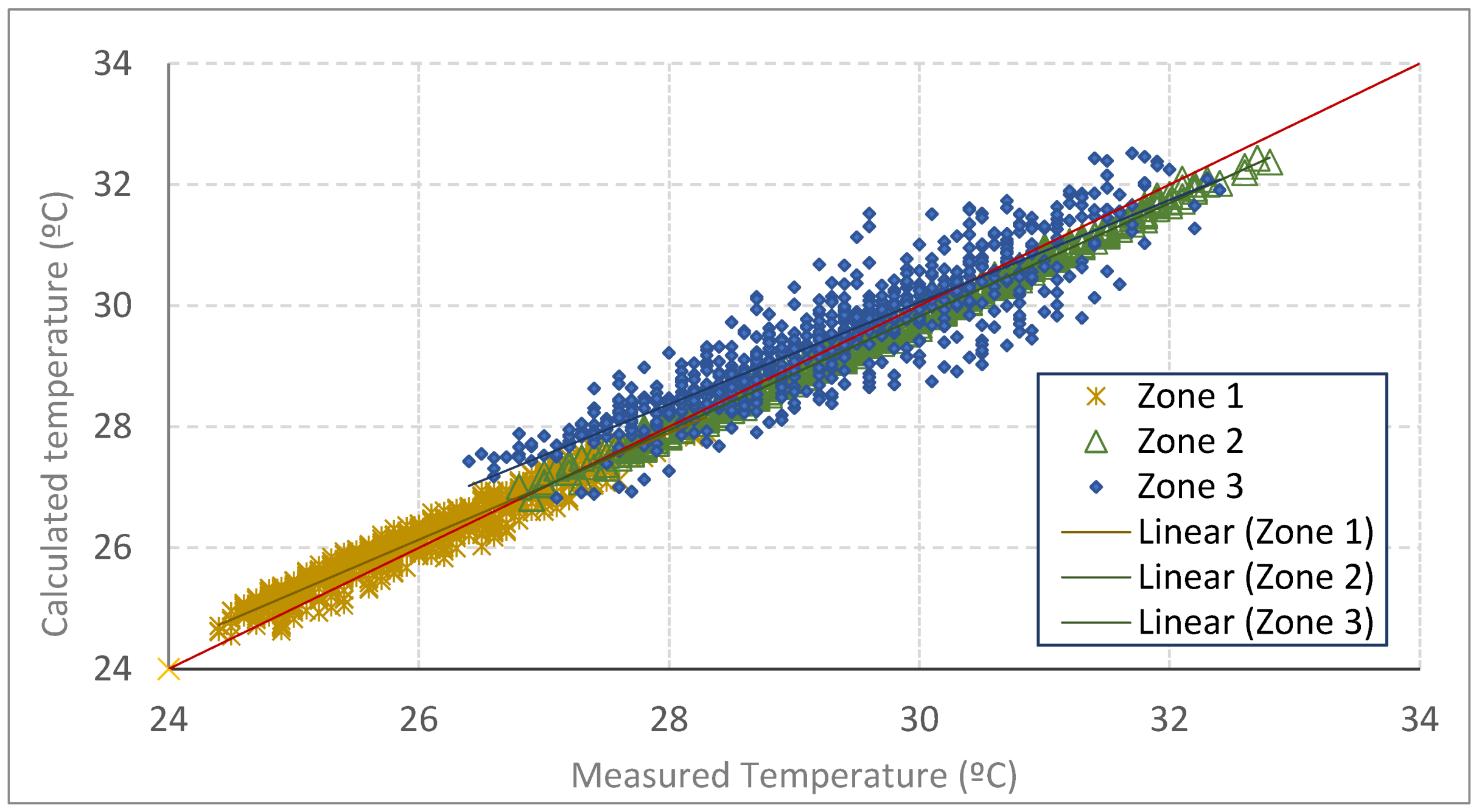
3.2. Model Validation

The monitoring data obtained from the monitoring study described in Section 2.2. were used to calibrate and validate the building model. The weather data file used in Design Builder was adapted, taking into consideration the actual outdoor conditions recorded during the monitoring period. Additionally, different values were assumed for the validation routine in the case of other parameters that play a role in the thermal performance of the building but whose precise evolution is more complex to register during the monitoring period. Thus, up to 48 different parameter combinations were simulated and evaluated in the validation process, assuming different scenarios for occupation (0–8 W/m²), infiltration (0–1 ach) and internal gains (0–10 W/m²). Indoor temperature was assumed as the indicator to evaluate the accuracy of the different combination evaluated. The adjustment of the combination selected for the main zones evaluated (see Section 2.2.3) is depicted in Figure 3. In it, the point clouds of each zone and their respective regression lines are shown, as well as the reference line x = y. Additionally, some relevant statistical indicators for each zone are presented in

Table 3. Statistical indicators of the model.

Data Set	R2	Intercept (a)	Slope (b)	CV_RMSE	Mean_Temp	Xc	Residual_SE
Zone 1	0.9386	3.2388	0.8807	0.72%	26.13 °C	27.15	0.19 °C
Zone 2	0.9935	1.7033	0.9372	0.31%	29.54 °C	27.12	0.10 °C
Zone 3	0.8067	4.7755	0.8427	1.67%	29.47 °C	30.36	0.49 °C

. Namely, the following values are presented for each data set: the R², intercept (a) and slope (b) of their corresponding regression lines; the Coefficient of Variation of the Root Mean Square Error (CV-RMSE) and the mean temperature of the data set. Two additional indicators are provided in the table: the X_c value and the Residual Standard Error. These two parameters are related to the systematic and random errors, respectively. The X_c value indicates the value where the regression line intersects with x = y, (i.e., where the systematic error of the regression becomes 0), whereas the Residual Standard Error is an indicator of the random error, a parameter that allows for determining the confidence interval in which the actual value is to be found. In that sense, the total error for any value of temperature is determined by the sum of the systematic error ± random error.

Based on these foundations, it could be observed that for the combination selected, the best adjustment is for “Zone 2”, although “Zone 1” and “Zone 3” also display acceptable results considering the purpose of this study and the range of the temperature values observed (between 24 °C and 33 °C). Although the intercept is relatively high (as shown in Table 3), the slopes of the regression lines are close to 1, and the three regression lines intersect x = y in the evaluated range (X_c). In a more detailed analysis of the systematic error, it can be calculated for each regression line, as presented in Equation (1), where “a” is the intercept, b is the slope, and “x” is the temperature value where the systematic error want to be calculated. It can be observed that within the temperature range considered, the regression lines present a maximum systematic error of 1.00 °C for the lowest values of temperature and −0.70 °C for the highest values of the range (Zone 3 and Zone 1, respectively).

$$Syst.Erro{r}_x=a+\left(b-1\right)·x$$

(1)

Additionally, the temperature profiles (measured and calculated) for the three zones are depicted in Figure 4. Overall, it can be observed that the model adequately represents the patterns observed in real measurements, with a sensible overestimation of temperatures. Zone 2 shows a better fit, especially under high-radiation conditions, but the results obtained for Zones 1 and 3 can also be considered acceptable. Although there are small deviations, the model proves to be accurate enough for the purpose targeted in this research work.

3.3. Scenarios Evaluated

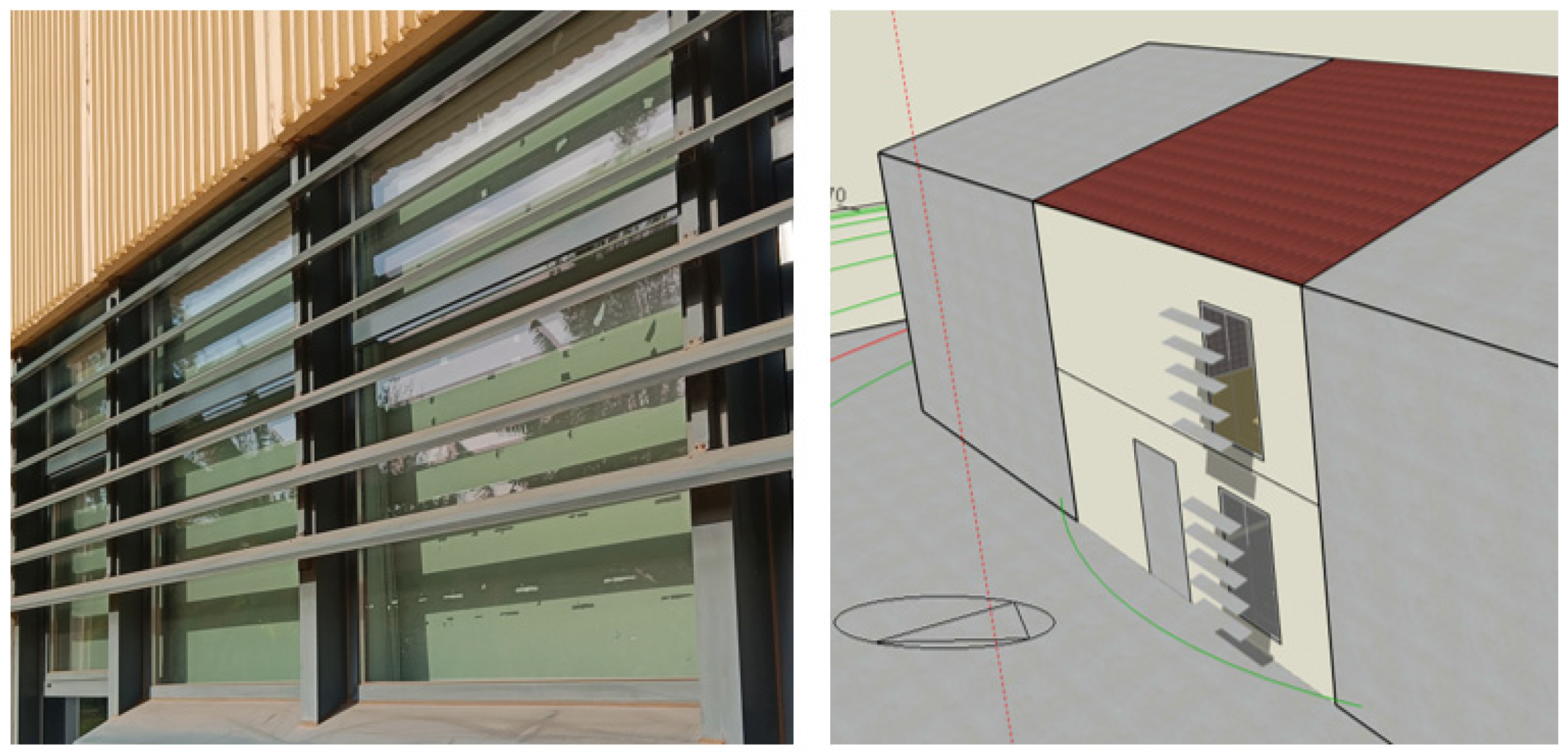
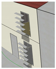
Once the model was validated, different simulation scenarios were defined with the aim of evaluating the impacts of different strategies. Besides the reference case, which was simulated to define a comparison point for the rest of the scenarios, four different strategies were assessed: louvers, overhangs in windows, overhangs in façades and side fins in windows. All strategies are evaluated individually, and additionally, a combination including louvers and side fins is also taken into consideration.

3.3.1. Louvers

The implementation of louvers is one of the strategies evaluated. Different parameters interact in the design of louvers, such as the number of blades, the vertical spacing between them, the blade angle and depth, and the position of the blades relative to the windows. In this case, two of them were assessed: the number of blades and the blade depth. As far as the number of blades is concerned, 2-blade and 5-blade scenarios were considered. Regarding the blade depth, 0.1, 0.15 and 0.25 cm were considered. Thus, six scenarios were defined for this strategy, resulting from the combination of these two parameters. The vertical spacing between blades (30 cm), the blade angle (15°) and the distance from window (30 cm) were assumed to be the same in all of these scenarios, as well as no vertical offset from the windows to blades nor horizontal window overlap (see Figure 5).

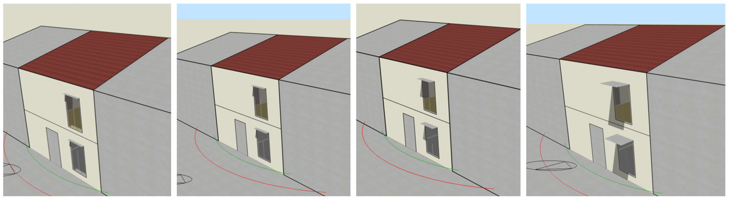
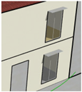
3.3.2. Overhangs (Windows)

The impact of installing local overhangs in all windows was also evaluated in this study. In this case, unlike the case of louvers, the parameters that play a key role in the energy performance of the building are more limited. Thus, the most relevant parameter to be considered in the case of overhangs for windows, apart from their position relative to the windows, is the length of the overhang (projection). Four different options for this parameter were evaluated—10 cm, 15 cm, 25 cm and 50 cm—resulting in the corresponding four scenarios for this strategy. Following a criterion analogous to the case of louvers, no vertical offset from the windows nor horizontal window overlap were assumed (see Figure 6).

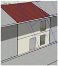
3.3.3. Overhangs (Façade)

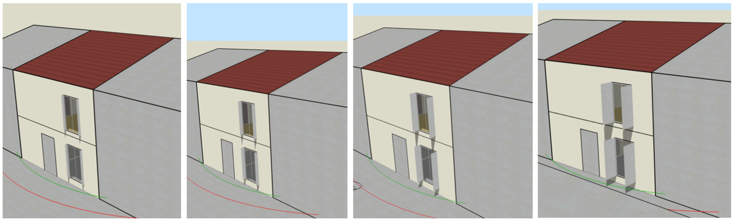
In this third scenario, an overhang for the whole façade is considered. As in the case of local overhangs for windows, the most relevant parameter is the length of the overhang. Being a structural element linked to the façade, longer lengths than in the previous strategy are considered in this case. Thus, three options were considered in this case: 30 cm, 50 cm and 1 m. As an example, in Figure 7, the shading effects of the different overhang lengths are shown, considering the sun position on the 1 July at 11:00 h.

3.3.4. Side Fins

The impact of vertical elements located in the sides of the windows (side fins) was evaluated in this fourth strategy. Like in previous cases, the main parameters, when defining a side fin, can be classified into two groups: those related to the element geometry itself and those related to the relative position of the element with respect to the window. Applying an equivalent criterion to the previous cases, no vertical offset from the windows nor horizontal window overlap were assumed, and the parameter evaluated in this case was the length of the element (“projection”), where four different options where considered: 10 cm, 15 cm, 25 cm and 50 cm (see Figure 8).

3.3.5. Combinations Evaluated

In short, a total of 23 possible combinations (24, when the baseline case scenario, with no shading element, is also taken into account) resulted from the different alternatives considered for each strategy evaluated. It should be noted that besides the evaluation of the aforementioned strategies independently, the effect of combining louvers and side fins was also assessed in this study. Each combination is codified by an alphanumeric code following the criteria presented in

Table 4. Summary of the strategies and variants evaluated.

	Louvers (L)	n = 2 (L − 2)	0.1 m (a)	0.15 m (b)	0.25 m (c)
		n = 5 (L − 5)	0.1 m (a)	0.15 m (b)	0.25 m (c)
	Overhangs, windows (OW)		0.1 m (a)	0.15 m (b)	0.25 m (c)	0.5 m (d)
	Overhangs, façade (OF)		0.3 m (a)	0.5 m (b)	1 m (c)
	Side fins (SF)		0.1 m (a)	0.15 m (b)	0.25 m (c)	0.5 m (d)
	Louvers + side fins		0.1 m (L − 2 + SFa)	0.15 m (L − 2 + SFb)	0.25 m (L − 2 + SFc)
			0.1 m (L − 5 + SFa)	0.15 m (L − 5 + SFb)	0.25 m (L − 5 + SFc)

. Thus, as an example, combination L5b indicates that this scenario considered louvers with 5 blades and a blade depth of 0.15 m.

3.4. Extrapolation of Results to Other Conditions: Different Orientations and Climates

These 24 combinations were also evaluated considering four different orientations (north, south, east and west). The resulting 96 combinations (24 variants × 4 orientations) were evaluated considering 5 different locations representative of different Colombian climate areas: the actual location of the case study, Bucaramanga in Santander, as well as Cali, Bogotá, Barranquilla and Medellín (see Figure 9). Finally, two climatic conditions were considered: the current climate data for every location and the expected future climate data for these locations as a consequence of one of the representative concentration pathways projected by the IPCC, namely the RCP 4.5. These RCPs (representative concentration pathways) describe possible future greenhouse gas emission scenarios, i.e., they are predictions of how these concentrations of greenhouse gases in the atmosphere will change in the future as a result of human activities. Different scenarios were defined, based on an effort to curb the carbon emissions, and RCP 4.5 is one of the intermediated scenarios defined in the Fifth Assessment Report [25]. In a climate change scenario, where significant changes are expected in the coming decades, this last point is relevant, since this additional analysis makes it possible to assess the level of sensitivity to climate variations of the three RQs addressed in this study and, consequently, determine whether changing climatic conditions would affect the effectiveness of the measures assessed over their lifetime. Thus, a total of 960 combinations were simulated.

3.5. Design of Simulations

The Eppy [26] and Geomeppy [27] Python libraries were used in this study to automate the generation and simulation of 960 building energy cases, utilising Python 3.7. This approach builds upon previously established processes used to handle large-scale energy simulations efficiently [23].

Initially, the reference building model was used to create a base set of 24 Input Data Files (.idf), comprising the original building configuration under its default orientation and climate, along with 23 combinations of shading strategies. These files were generated using Design Builder software and exported for EnergyPlus compatibility.

The automation process, carried out through Python scripting, systematically adjusted the orientation of each of the 24 base .idf files and applied the corresponding climate file for the simulation. Each orientation was simulated across ten climate data sets—five locations under two climate scenarios, current climate and future climate projections—based on the IPCC’s RCP 4.5 scenario.

This setup resulted in 960 unique cases. Additionally, each case was simulated with and without cooling systems, yielding a total of 1920 simulations. The automation workflow included two main steps:

• A Python script modified the .idf files iteratively for each scenario, accounting for orientation and building location. Simulations were then conducted for each iteration.
• The simulation outputs were processed and compiled into spreadsheets containing monthly cooling demands and the total annual cooling demand (in kWh) for each simulated case.

3.6. Data Analysis

As previously mentioned, two different packages, each composed of the 960 simulation scenarios, were run in Design Builder. In the first package, the simulations were run assuming an indoor cooling set point of 24 °C, with the aim of analysing the evaluated strategies considering the cooling demand (yearly and monthly) required to maintain the home below 24 °C. In that sense, the more efficient a given strategy is, the less energy demand will result. In the second case, the simulations were carried out assuming no cooling set point to evaluate the indoor thermal conditions resulting from applying the different shading strategies when no cooling system is in the building. This allows for evaluating the impact of the evaluated strategies considering both indicators: “theoretical” cooling demand (the amount of energy required in each case to keep stable a given indoor temperature) and indoor comfort conditions when no cooling system exists in the house (as is the case in many residential buildings).

Based on this design of the simulations, the results are analysed in two different phases. Firstly, the results obtained from the first package are evaluated considering the resulting yearly cooling demands. These yearly cooling demands are evaluated firstly through a factorial Analysis of Variance (ANOVA) to compare the shading strategies evaluated and to what extent they are significantly different from each other. To do this, in the first phase, the four variation factors (location, orientation, strategy and climate) and their interactions are considered. Scenarios were grouped by strategy in such a way that scenarios corresponding to different variants of a given strategy were considered as repetitions. Thus, the different scenarios evaluated were organised into 7 different categories according to the shading strategy assessed (see Table 4): 2-blade louvers (L2); 5-blade louvers (L5); overhangs, windows (OW); overhangs, façade (OF); side fins (SF); 2-blade louvers and side fins (L2-SF) and 5-blade louvers and side fins (L5-SF). Then, the values were compared using Tukey’s mean separation test.

As far as the mean separation tests are concerned, they allow for the classification of the differences between the different levels evaluated in a source (in this case, the seven categories previously mentioned), determining which are significant and which are not. To do this, all possible pairs of mean values are compared with each other. These tests group the different levels evaluated according to the differences between them so that the mean values that do not show a significant difference (for a previously established significance level α) are included in the same category. Thus, in this study, the mean separation test makes it possible to determine which strategies present differences that can be considered significant. Different methodological proposals for the separation of means test can be found from different authors (e.g., Scheffé, Duncan, Dunnett or Tukey). In this case, Tukey’s mean separation test was selected.

For the data curation, “R” software (version 4.4.2) was used [28], as well as two of its specific libraries: “stats” for ANOVA (integrated in the R base package) and “agricolae” [29] for Tukey’s mean separation tests. In the case of the latter, it has been developed using the HSD.test function of the mentioned “agricolae” package, whose detailed procedure can be found in [29].

Additionally, with the aim of evaluating and identifying the optimal and most effective shading strategies, the cooling demand savings of each scenario are calculated by subtracting the resulting cooling demand in a given scenario to the cooling demand obtained for the corresponding baseline scenario. This baseline scenario would be the reference case scenario, being in the same location and with the same orientation. This approach, together with the aforementioned ANOVA study, allows for analysing to what extent the location and orientation are relevant parameters when deciding the most efficient shading strategies or, in contrast, if there are strategies that perform better than others regardless of the location and orientation where they are to be implemented.

From these analyses, a set of representative scenarios are selected to carry out a detailed analysis about the implications of them on indoor thermal comfort. These implications are analysed by means of the calculation of the thermal sensation index by using the procedure proposed by the IDEAM [30]. This method calculates the heat sensation and thermal comfort based on the adjusted equation of cooling power proposed by de Leonardo Hill y Morikofer-Davos, and it has been used in other research works, e.g., [31]. In this case, it aims to calculate a Comfort Index (CI) instead of cooling power, considering the air temperature, relative humidity and air velocity, as well as altitude (identifying three different groups: locations under 1000 m, locations between 1000 and 2000 m and locations higher than 2000 m) as the main input parameters. Based on the CI obtained, seven different categories are defined: excessively hot, hot, warm, comfortable, cool, cold and excessively cold. The workflow, as well as the main equations used to calculate the IC, are presented in Figure 10.

4. Results and Discussion

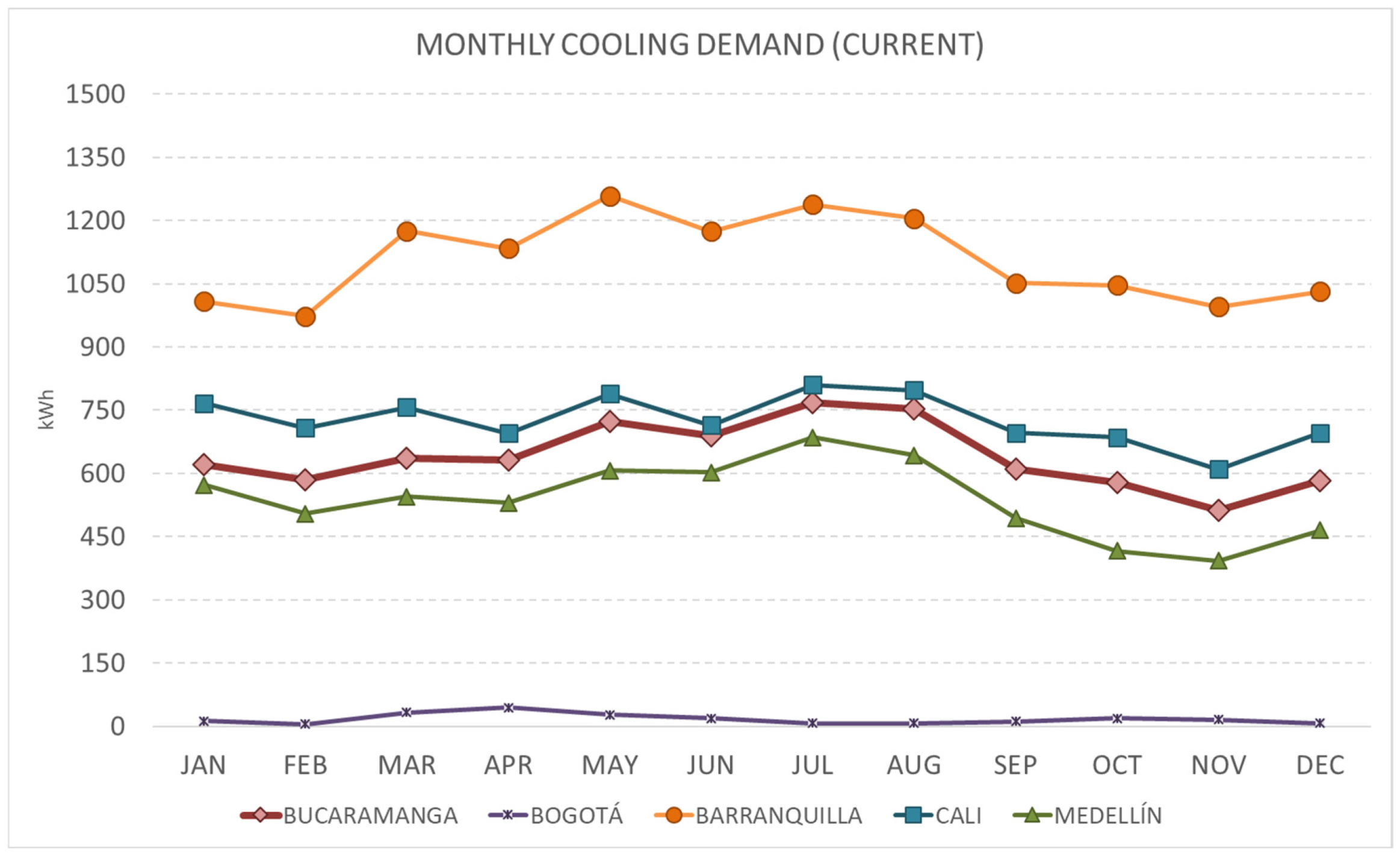
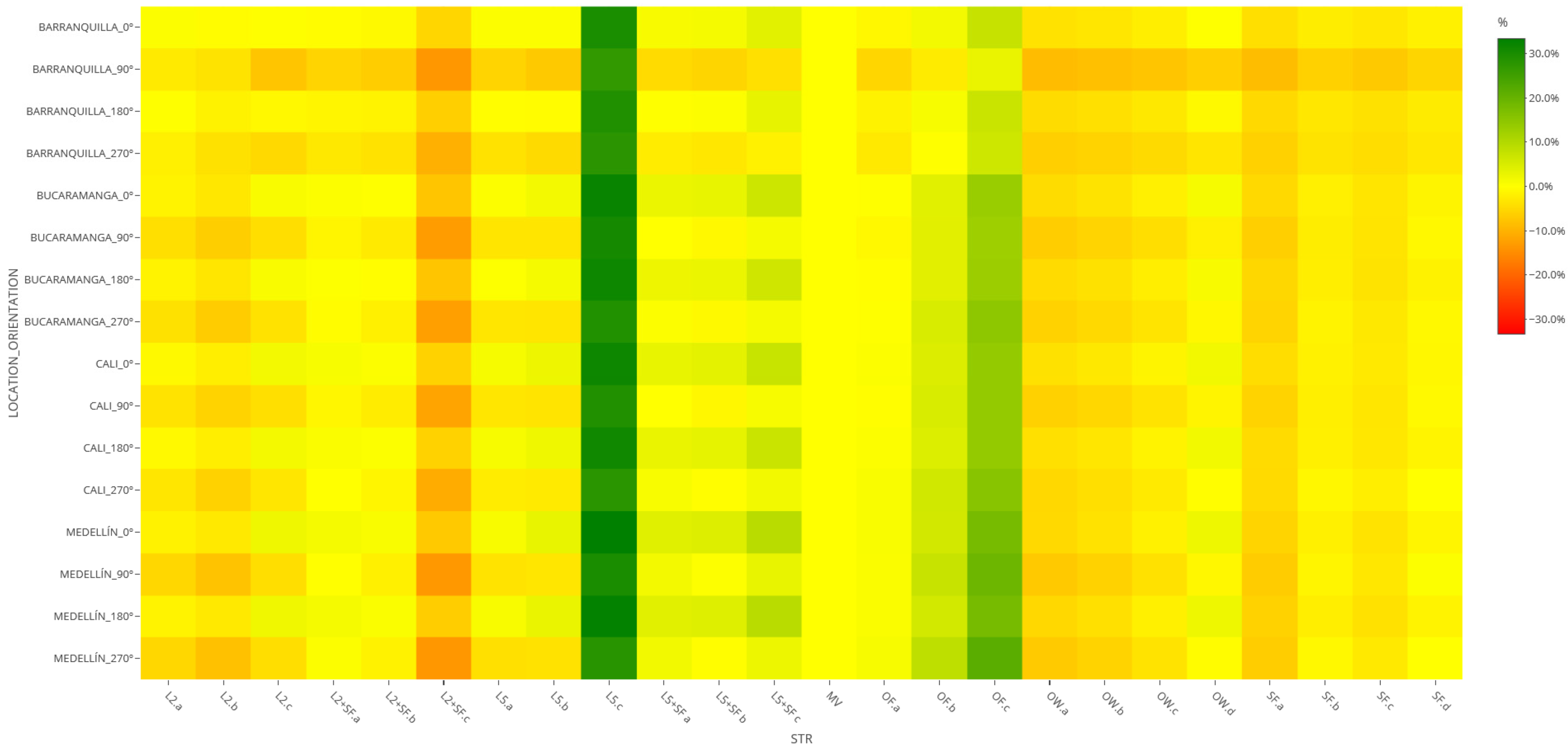
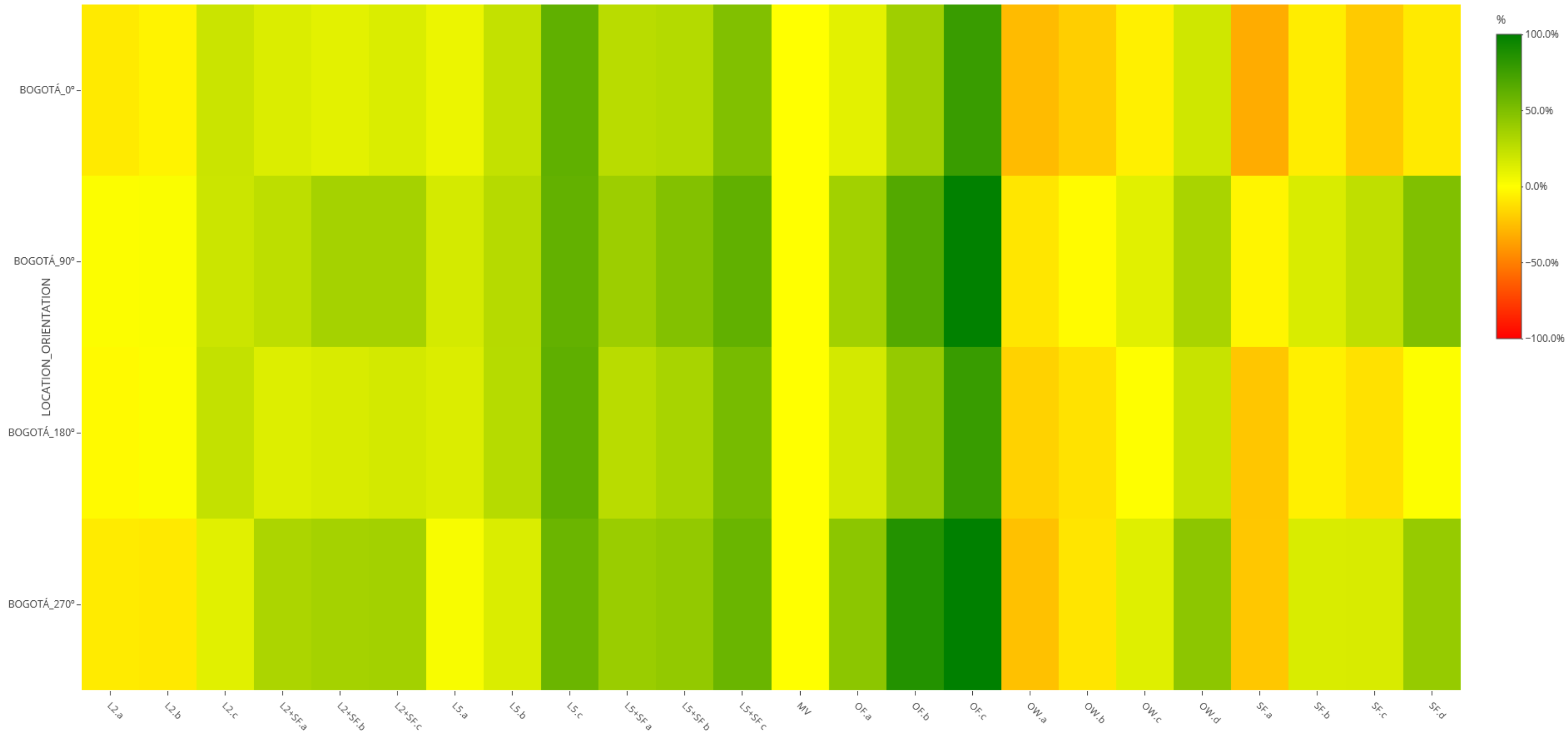
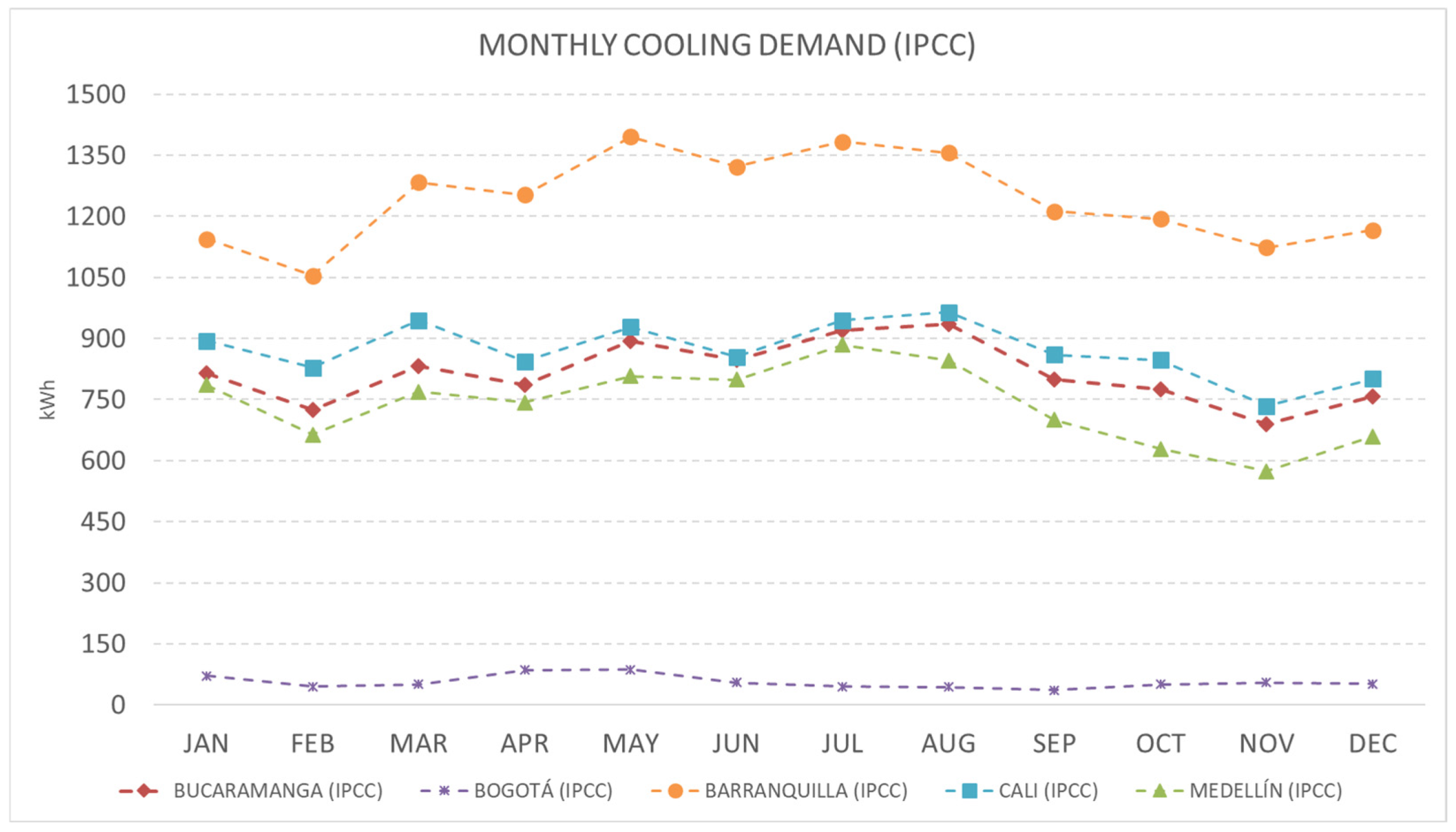
All results obtained from these simulations are publicly available in [16]. In this paper, as previously mentioned, the results are presented and analysed considering two different approaches. Firstly, the theoretical cooling demand of all simulated scenarios is evaluated. Then, the impact on indoor thermal comfort is evaluated. To do this, the most effective strategies identified in the analysis of the cooling demands are selected to be analysed in detail. Finally, the impact of climate change is also taken into consideration in this study by evaluating the expected evolution of these results considering the future climate scenario RCP 4.5 projected by the IPCC.

4.1. Cooling Demand

Monthly and yearly cooling demands were obtained from all scenarios evaluated. When analysing the monthly demand (as an example, the monthly cooling demands for the baseline case scenario in the five locations is presented in Figure 11), it can be observed that the five locations considered (Bucaramanga, Bogotá, Cali, Barranquilla and Medellín) show a profile where the cooling demand is distributed over the whole year. Additionally, the evaluated locations can be classified into three different groups according to their cooling demand profile: Bogotá, with an almost negligible cooling demand during the whole year (an aggregated value of 209.32 kWh/year, i.e., 1.46 kWh/m².year); Barranquilla, with monthly cooling demands ranging from 970 kWh/month to 1250 kWh/month (13,291.3 kWh/year, i.e., 105.49 kWh/m².year) and a third group formed by the Cali, Medellín and Bucaramanga scenarios, showing aggregated yearly values ranging between 50 and 70 kWh/m².year (51.25 kWh/m².year in Medellín, 61.03 kWh/m².year in Bucaramanga and 69.24 kWh/m².year in the case of Cali).

Once the reference scenario is characterised, the impact of the different parameters considered (orientation and location) in the optimal design of the shading strategies evaluated is analysed. Thus, with the aim of answering one of the research questions outlined in this work (namely RQ2), a set of factorial ANOVA analyses are carried out, considering, in this case, the yearly cooling demands obtained from the simulation of the scenarios evaluated.

In the first ANOVA, the yearly cooling demands of the 960 scenarios are included, and the four variation factors (location, orientation, strategy and climate) and their interactions are considered. In this first stage, significant differences are found for the four independent factors and for the three double interactions where the “location” factor takes part (α = 3.3 × 10⁻⁶ for “location: strategy” and α < 2.2 × 10⁻³⁴ for the rest of the interactions). Neither the rest of the double interactions nor the triple or quadruple interactions show significance (α > 0.45).

In a second phase, an additional ANOVA is carried out, focusing on the factors and interactions identified as significant in the first phase. Taking into account the significant interactions, the data set is itemised, and additional ANOVAs are carried out at different levels until non-significant interactions or single-factor ANOVAs are obtained. The main outcomes of this analysis are presented in

Table 5. ANOVA of the whole data set generated (yearly cooling demand values).

Source	Df	Sum Sq	Mean Sq	F Value	Pr(>F)	Sign
LOCATION (LOC)	4	1.60 × 1010	4.10 × 109	1.70 × 104	0.00 × 100	***
CLIMATE (CLI)	1	6.10 × 108	6.10 × 108	2.50 × 103	1.20 × 10−264	***
STRATEGY (STR)	7	9.50 × 107	1.40 × 107	56.62	3.30 × 10−67	***
ORIENTATION (ORI)	3	4.30 × 108	1.40 × 108	600.54	3.00 × 10−214	***
LOC:CLI	4	1.20 × 108	2.90 × 107	120.29	3.10 × 10−82	***
LOC:STR	28	2.50 × 107	9.10 × 105	3.78	2.90 × 10−10	***
LOC:ORI	12	7.20 × 107	6.00 × 106	24.9	1.50 × 10−48	***
Residuals	900	2.20 × 108	2.40 × 105	NA	NA
Total	959	1.80 × 108	NA	NA	NA

Level of significance: α = 0 ‘***’; α = 0.001 ‘**’; α = 0.01 ‘*’; α = 0.05 ‘.’; α = 0.1 ‘ ’; α = 1.

, where for each source of variation (factors, interactions and residuals), the following data are presented: degree of freedom (Df), sum of squares (Sum Sq), mean square (Mean Sq), F value, p value (Pr(>F)) and significance (sign) based on the α value. From this analysis, it is determined that all cases shown a high significance level (α < 2.9 × 10⁻¹⁰), with an R² of 0.988.

In a more detailed analysis of the locations, it can be identified that Bogota is the location that shows the most different performance compared to the other locations, and it is identified as a cause of the identified interactions. Thus, two new ANOVAs are carried out: one considering only the results of Bogotá scenarios and the other considering the rest of scenarios. Hence, a new ANOVA is carried out in the data set excluding Bogotá, as shown in

Table 6. ANOVA of the data set generated, excluding scenarios located in Bogotá (yearly cooling demand values).

Source	Df	Sum Sq	SS %	Mean Sq	F value	Pr(>F)	Sign
LOCATION (LOC)	3	4.60 × 109	74.72%	1.50 × 109	5.10 × 103	0.00 × 100	***
CLIMATE (CLI)	1	7.10 × 108	11.48%	7.10 × 108	2.30 × 103	2.70 × 10−233	***
STRATEGY (STR)	7	1.10 × 108	1.84%	1.60 × 107	53.85	2.60 × 10−62	***
ORIENTATION (ORI)	3	5.00 × 108	8.05%	1.70 × 108	549.25	9.60 × 10−189	***
LOC:CLI	3	1.50 × 107	0.25%	5.10 × 106	17.01	1.10 × 10−10	***
Residuals	750	2.30 × 108	3.66%	3.00 × 105	NA	NA
Total	767	6.20 × 109	100.00%	NA	NA	NA

Level of significance: α = 0 ‘***’; α = 0.001 ‘**’; α = 0.01 ‘*’; α = 0.05 ‘.’; α = 0.1 ‘ ’; α = 1.

. In this case, it is found that the four factors present a high significance level, as well as only one interaction (location: climate). Neither strategy nor orientation yield significant interactions with any of the other factors. This involves that a joint analysis of all the results obtained for the four locations can be carried out in order to analyse the behaviours of the different strategies considered, as well as the effect of the orientations on the cooling demand. Likewise, the absence of significant interactions confirms that the selection of optimal strategies will be independent of orientation, climate and location. In other words, the strategy with the best performance in one of the locations considered will also perform best in the other three locations.

Subsequently, with the aim of addressing RQ1 (“What is the optimal design of different shading solutions for latitudes close to the equator?”), the values comprising this data set are compared using Tukey’s mean separation test. In this case, a significance level of α = 5% was assumed. The results of this test are summarised in

Table 7. Results of Tukey’s mean separation test (by strategy).

Strategy	Mean Value
2-blade louvers + side fins (L2 + SF)	9385.29	a
Overhang, windows (OW)	9349.78	a	b
Side fins (SF)	9347.52	a	b
2-blade louvers (L2)	9242.59	a	b
No shading (reference case)	9033.61		b	c
5-blade louvers + side fins (L5 + SF)	8946.82			c
Overhang, façade (OF)	8679.14				d
5-blade louvers (L5)	8247.23					e
Significance level α = 5%

, where the different levels (in this case, strategies) are grouped based on the differences between them, as previously presented in Section 3.6. It can be observed that five main groups are identified in terms of significance. There is a set of four strategies (L2 + SF, OW, SF and L2) which, on average, perform worse than the reference case scenario, even though, except in L2 + SF, the differences cannot be considered significant. On the other side, the values obtained for “louvers” and “overhangs-façade” show significant differences (they show lower cooling demands on average, i.e., perform slightly better) when compared to the reference case and even between them. The table also shows that the reference case scenarios (“no shading”) do not yield significant differences with L5 + SF nor OW, SF and L2 (the groups categorised as b and c), which indicates that it cannot be dismissed that the existing differences, from an statistical point of view and based on the used data, are due to random effects. When the same procedure is applied based on orientation, it is also observed that two main groups are similarly identified, corresponding to the north and south orientation and the east and west orientation, respectively.

In short, this three-stage process (ANOVA of the whole data set; ANOVA of the data set excluding scenarios located in Bogotá; Tukey’s mean separation test), show that except in the case of Bogota, due to its specific climate conditions and low cooling demand values, there are significant differences from a statistical point of view when the general performance of the different strategies considered is evaluated. Based on these findings and with the aim of analysing the variants of each strategy in a more detailed way, a new indicator is calculated for each scenario: the percentage of savings of cooling demand for each variant comparing to the reference case study (“no shadings”) located in the same location and with the same orientation. This analysis also aims to partially address RQ3 (“What impact do these measures have in terms of cooling demand reduction and thermal comfort?”). This percentage of savings is calculated as the difference between the cooling demand of the reference case (same location and same orientation) and the cooling demand of the given scenario in such a way that positive values mean energy savings related to the strategy and variant considered, and negative values mean that the evaluated scenario increases the cooling demand comparing to the reference case.

The results are depicted in the heat map shown in Figure 12, where the green colour represent savings. For the sake of the clarity, also in this case, Bogotá-related data are presented separately (in Figure 13), since, due to the different performance of the scenarios located in Bogotá, the range of the values obtained for them presents important differences with the rest of the scenarios, and including these values in the same heat map would make the analysis of the heat map more complex (the differences between the scenarios in the other locations would become blurred as a result of the weighting of the Bogotá scenarios). As shown in Figure 12, there are some variants with savings regardless of orientation and location, namely L5c (louvers, five blades and a blade depth of 0.25 m; see Table 4) and OFc (overhang in the façade of 1 m length), showing savings ranging from 26.7% (Barranquilla, 90°) to 33.3% (Medellín, 0°) and from 2.8% (Barranquilla, 90°) to 21.5% (Medellín, 270°), respectively. As can also be observed in Figure 13, similar conclusions can be obtained in the case of the scenarios located in Bogotá; even though, in this case, more variants show better values of relative savings in cooling demand (to some extent due to the absolute values of yearly cooling demand compared to the rest of the locations), L5c and OFc stand out as the best performing variants. This is clearly aligned with the previously presented results yielded by Tukey’s mean separation test, and this confirms the insights of that test.

The impact of overhangs in the façade, being significantly higher than the other strategies evaluated, can be explained to some extent by the reduction in solar radiation that not only the windows, but also the whole façade, experience during some periods of the daytime (Figure 7 is an illustrative example of this). This effect involves a reduction in the overheating of the outer surface of opaque elements and, as a consequence, results in lower heat gains through the façade, which become relevant considering their high U-value (2.32 W/m²·K). It should be noted that this effect could be reduced in the case of buildings with low U-values of the façade, where heat gains through the opaque walls are less significant in the global energy balance of the building. In contrast, side fins show to be ineffective regardless of the orientation and location considered, mainly as a consequence of the sun path in the latitude evaluated (see Figure 8 as an illustrative example of the resulting shading)

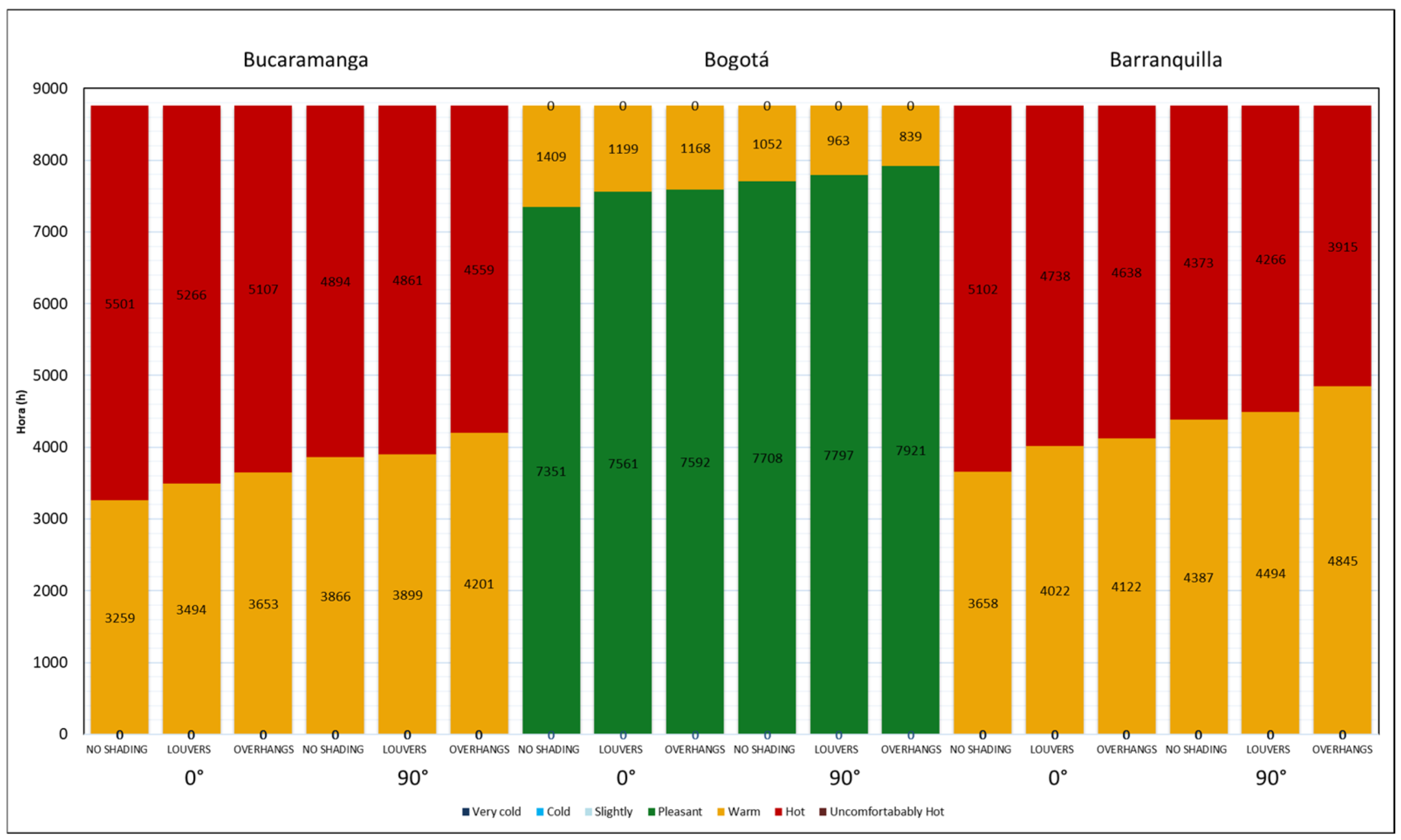
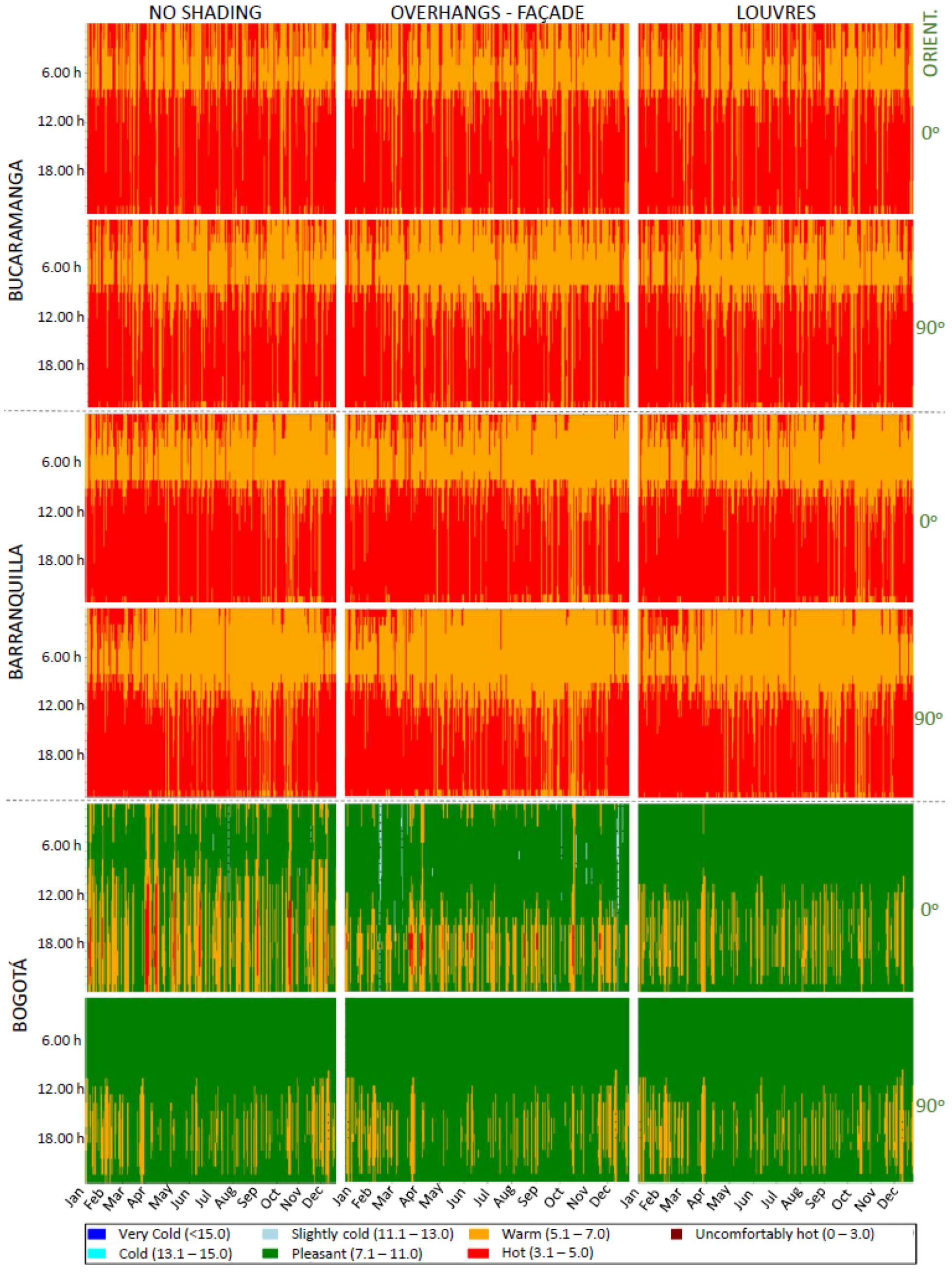
4.2. Indoor Comfort Analysis

Based on the results obtained from the cooling demand analysis and visualised in the percentage savings graphs, the indoor comfort analysis of the two variants previously identified as the best performing ones (L5c “louvers” and OFc “Overhang-façade”) are presented in this section. The analysis also includes the base scenario for these locations (“no shading”) as a reference to evaluate, via a comparison, the improvements of the strategies. It should be noted that the indoor comfort results of all scenarios evaluated are also publicly available in [16].

Moreover, for the sake of clarity, the analysis presented in this section focuses on three of the locations evaluated, considered as representative, as previously described in Section 4.1: Bucaramanga, Bogotá and Barranquilla. These cities were chosen for their contrasting climatic profiles and specific energy demands. Bucaramanga represents a warm–moderate climate (representing similar conditions to Cali and Medellín), Bogotá is characterised by its cold climate and low cooling requirements, and Barranquilla reflects the extreme conditions of a warm–humid climate. Additionally, two orientations were evaluated in this case as the most representative: the original orientation of the case study, east–west (0°), and the north–south orientation (90°).

Following the method presented in Section 3.6, the Comfort Index is used as an indicator to perform the indoor comfort analysis, being calculated according to the equations presented in Figure 10. As shown in Figure 14, where the number of thermal sensation hours is also calculated for the selected cases for Bucaramanga, Bogotá and Barranquilla, the analysis of these cities reveals significant differences in thermal comfort conditions, influenced by the specific climatic characteristics of each location and the orientations of the implemented strategies. It should be noted that the results are based on data related to the ground floor, considered the reference level for this analysis.

In Bucaramanga, the shading strategies demonstrate a significant reduction in hours classified as “uncomfortably hot.” Without shading, these hours account for a substantial portion of the annual time, with 5501 h at an orientation of 0° and 4559 h at orientation 90°. The implementation of “louvers” reduces these hours by 4% for 0° and 12% for 90°, while “overhangs-façade” achieves reductions of 7% and 17%, respectively. These percentages are calculated by comparing the hours of each implemented strategy against the “no shading” reference model. This effect results in a redistribution of hours towards the “warm” range, reaching 4894 h with “overhangs-façade” at 0° and 3866 h at 90°, thereby enhancing indoor thermal comfort.

In Bogotá, passive strategies have a significant effect on the transition of hours from the warm range to the comfortable range. Without shading, warm hours reach values of 1199 at the orientation 0° and 839 at 90°, while comfortable hours exceed 90% of the annual time. The implementation of “louvers” and “overhangs-façade” increases the comfortable hours by 15% to 17% at an orientation of 0° and by 32% to 40% at 90°, reaching up to 7921 h with “overhangs-façade.” These percentages are also calculated by comparing each strategy with the reference model, demonstrating their ability to optimise the thermal conditions.

Finally, in Barranquilla, the shading strategies show a significant reduction in hot sensation hours, which, without shading, reach 5102 h at an orientation of 0° and 3915 h at 90°. “Louvers” reduce these hours by 7% at 0° and 16% at 90°, while “overhangs-façade” achieves reductions of 10% at 0° and 23% at 90°. These percentages are derived by comparing the values with the “no shading” model.

In Bucaramanga, the “no shading” scenario shows a predominance of hours in the “uncomfortably hot” range, reaching 5501 h in the 0° orientation and 4559 h in the 90° orientation. The implementation of shading strategies such as “louvers” and “overhangs-façade” significantly reduces these hours, increasing those in the “warm” and “pleasant” ranges. These strategies prove effective in mitigating direct thermal gains, with consistent results for both orientations. In Bogotá, the majority of hours are already within the “pleasant” range, even without shading, with over 7350 h in both the 0° and 90° orientations. Shading strategies like “overhangs-façade” and “louvers” further optimise these conditions, reaching up to 7921 “pleasant” hours in the 90° orientation. This indicates that although the impact in this city is more moderate, these strategies help maintain favourable thermal comfort conditions for longer periods. Finally, in Barranquilla, characterised by its warm–humid climate, the “no shading” scenario presents a high number of hours in the “uncomfortably hot” range, with 5102 h in the 0° orientation and 3915 h in the 90° orientation. Shading strategies, particularly louvers, significantly reduce these hours, increasing those in the “warm” and “pleasant” ranges. This is particularly notable in both orientations, where passive strategies prove essential for improving thermal comfort in extreme conditions. Additionally, in a more detailed comparison, the time distribution of the heat index is presented in the hourly-based graphs depicted in Figure 15. In these, it can be observed that in the case of Barranquilla and Bucaramanga, there is, in general and in both orientations considered, a sensible increase in the number of hours categorised as “warm” by reducing the number of hours classified as “hot” (graphically, an increase in the orange area to the detriment of the red area). In the case of Bogota, changes are slighter but not less significant. Particularly, in the east–west orientation (0°), the number of hours classified as hot (red) is significantly reduced in the case of the “overhang, façade” scenario and becomes zero in the case of louvres. It is also noticeable that in the case of “overhang, façade”, some hours become “cold” (turquoise colour), mainly during the months of February, March, November and December. This issue could be a key element to conclude that in the case of Bogotá and at that specific orientation and assuming the current climate, louvres would be a better-balanced option compared to louvers when indoor comfort is taken into consideration.

The analysis highlights the effectiveness of passive shading strategies in improving thermal comfort across different climatic contexts and orientations. In warm climates, such as those of Bucaramanga and Barranquilla, strategies like “louvers” and “overhangs-façade” proved efficient in reducing overheating and promoting more comfortable thermal conditions. In Bogotá, characterised by its cold climate and lower cooling demand, these strategies help optimise existing thermal comfort conditions. The findings emphasise the importance of tailoring passive solutions to the climatic characteristics and orientation of each location, enhancing indoor comfort while supporting sustainable strategies in building design.

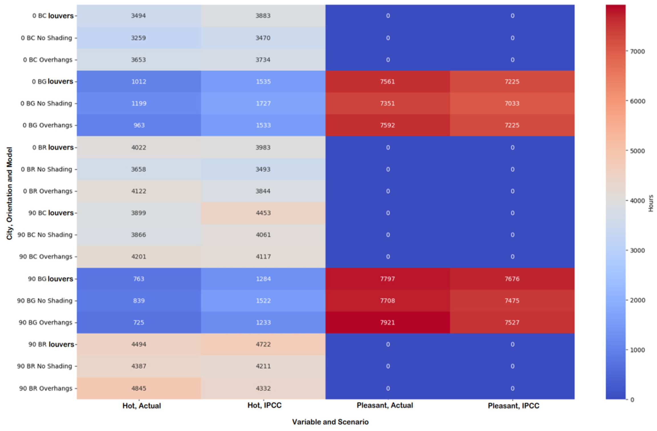
4.3. Future Climate Scenarios

Finally, the impact of these strategies in the context of climate change is also considered in this work. Thus, all strategies evaluated were also simulated assuming the climate conditions projected by the IPCC in the representative concentration pathway RCP 4.5 for the five different locations considered in this work.

As far as the impact on cooling demand is concerned, RCP 4.5 involves a significant increase in the cooling demand for all scenarios evaluated. As an example, the monthly cooling demands for the baseline case scenario in the five locations assuming this climate scenario are presented in Figure 16. It can be observed, when comparing with the current climate scenario (see Figure 11), that the monthly demand profile increases notably in all of them. In relative values, the most relevant increment is observed in Bogotá as a consequence of the low cooling demand values in absolute terms (an increment of the 222% in the yearly cooling demand, from 1.66 kWh/m².year to 5.35 kWh/m².year). In the other hand, Barranquilla yields an increment of 12% (from 105.49 kWh/m².year to 118.15 kWh/m².year). Cali, Bucaramanga and Medellín show intermediates values, namely 19.75%, 27.10% and 37.23%, respectively.

Regarding thermal sensation, Figure 17 presents the thermal sensation hours across the current and IPCC (RCP 4.5) scenarios, categorised by city, orientation and shading strategy. The rows represent the evaluated combinations, while the columns display thermal categories (“hot” and “pleasant”) under both scenarios. The colour scale highlights the projected changes, revealing increases in the “hot” hours and reductions in the “pleasant” hours, particularly in the absence of shading strategies.

In Bucaramanga, the IPCC scenario reveals significant increases in the “hot” hours under the “no shading” strategy, with increments of 211 h in the 0° orientation and 195 h at 90°. Shading strategies such as “louvers” and “overhangs” also exhibit increases in this range, particularly “louvers”, which shows increments of 389 h at 0° and 554 h at 90°. Although these strategies mitigate “uncomfortably hot” hours, the projected climate change shifts these hours toward the “hot” range, reducing the overall effectiveness of these solutions. This behaviour is also observed in Bogotá, where the impacts of the IPCC scenario are more pronounced, with a significant reduction in “pleasant” hours, replaced by increases in the “hot” range. Under “no shading,” “pleasant” hours decrease by 318 at 0° and 233 at 90°, while “hot” hours increase by 528 and 683, respectively. Shading strategies show similar patterns, although with less magnitude: with “louvers”, “pleasant” hours decrease by 336 at 0° and 121 at 90°, while “hot” hours increase by 523 and 521, respectively. Meanwhile, “overhangs” reduces “pleasant” hours by 367 at 0° and 394 at 90°, accompanied by equivalent increases in the “hot” range, emphasising the need to strengthen passive strategies to maintain thermal comfort conditions.

In contrast, Barranquilla exhibits a different behaviour, with “hot” hours showing slight reductions or marginal increases depending on the implemented strategy. Under “no shading,” “hot” hours decrease by 165 at 0° and 176 at 90°, while “uncomfortably hot” hours increase significantly. Shading strategies such as “louvers”, and “overhangs” help moderate these impacts, with “overhangs” reducing “hot” hours by 278 at 0° and 513 at 90°. However, these strategies face limitations under extreme climatic conditions, as “uncomfortably hot” hours remain elevated in the IPCC scenario, highlighting the need for additional strategies to mitigate the effects of climate change.

5. Conclusions and Future Works

This work has evaluated the effectiveness of different design variants of shading strategies in residential buildings in different Colombian climates. The impact of evaluated strategies on cooling demand and indoor comfort has been analysed. To do this, a representative typology was identified, a case study located in Bucaramanga (Santander) was monitored for one month, and the obtained monitoring data were used to validate and calibrate a building model defined using Design Builder software. Once the model was validated, a set of 960 scenarios resulting from a combination of different strategies, parameters and locations was simulated, and their results were analysed considering both cooling demands and indoor comfort conditions.

As far as the first research question defined at the beginning of this research piece (RQ1—What is the optimal design of different shading solutions for latitudes close to the equator?), the results shown the louvers and, specially, overhangs in façades, stand out as the most effective shading strategies to be applied at these latitudes, considering the building constructions and features of a representative typology of single-family buildings in the areas evaluated.

The detailed analysis of these results also yields that the two identified strategies show, in general, the best performance regardless of the orientation and location considered, answering, in this way, the second research question raised in this study (RQ2—What impacts do orientation and location have on the design of these strategies?). The main differences in this regard could be found in the case of Bogotá, due to its significantly colder climate conditions compared to the other four locations evaluated, even though similar trends were observed in this location.

Regarding the last research question contemplated in this work (RQ3—What impact do these measures have in terms of cooling demand reduction and thermal comfort?), the impact of some of the strategies evaluated seems to be negligible, but significant improvements are reported in the case of louvers and overhangs in façades, both in terms of cooling demands (reaching demand savings close to the 30% in the optimal variant of louvers) and indoor comfort conditions, reducing significantly the number of hours with an IC categorised as “hot” (e.g., close to 500 h in the case of Barranquilla when overhangs in façades are evaluated).

Finally, the research work has shown that considering the projections of future climate scenarios, the situation in terms of cooling demand and indoor comfort conditions is expected to be more critical. In that sense, the strategies evaluated show similar levels of effectiveness in relative terms, with louvers and overhangs again being identified as the best performing options also when future climate projections are assumed.

References

1. Vélez-Henao, J.A.; Pauliuk, S. Pathways to a Net Zero Building Sector in Colombia: Insights from a Circular Economy Perspective. Resour. Conserv. Recycl. 2025, 212, 107971. [Google Scholar] [CrossRef]
2. Ibrahim, M.; Harkouss, F.; Biwole, P.; Fardoun, F.; Ouldboukhitine, S. Building Retrofitting towards Net Zero Energy: A Review. Energy Build. 2024, 322, 114707. [Google Scholar] [CrossRef]
3. IPCC. Intergovernmental Panel on Climate Change Climate Change 2022: Impacts, Adaptation and Vulnerability. Contribution of Working Group II to the Sixth Assessment Report of the Intergovernmental Panel on Climate Change; Pörtner, H.-O., Roberts, D.C., Tignor, M., Poloczanska, E.S., Mintenbeck, K., Alegría, A., Craig, M., Langsdorf, S., Löschke, S., Möller, V., et al., Eds.; Cambridge University Press: Cambridge, UK; New York, NY, USA, 2022. [Google Scholar]
4. Medina, J.M.; Rodriguez, C.M.; Coronado, M.C.; Garcia, L.M. Scoping Review of Thermal Comfort Research in Colombia. Buildings 2021, 11, 232. [Google Scholar] [CrossRef]
5. Ríos-Ocampo, J.P.; Olaya, Y.; Osorio, A.; Henao, D.; Smith, R.; Arango-Aramburo, S. Thermal Districts in Colombia: Developing a Methodology to Estimate the Cooling Potential Demand. Renew. Sustain. Energy Rev. 2022, 165, 112612. [Google Scholar] [CrossRef]
6. Balbis-Morejón, M.; Cabello-Eras, J.J.; Rey-Martínez, F.J.; Fandiño, J.M.; Rey-Hernández, J.M. Energy Performance of a University Building for Different Air Conditioning (AC) Technologies: A Case Study. Buildings 2024, 14, 1746. [Google Scholar] [CrossRef]
7. Valladares-Rendón, L.G.; Schmid, G.; Lo, S.-L. Review on Energy Savings by Solar Control Techniques and Optimal Building Orientation for the Strategic Placement of Façade Shading Systems. Energy Build. 2017, 140, 458–479. [Google Scholar] [CrossRef]
8. Khourchid, A.M.; Ajjur, S.B.; Al-Ghamdi, S.G. Building Cooling Requirements under Climate Change Scenarios: Impact, Mitigation Strategies, and Future Directions. Buildings 2022, 12, 1519. [Google Scholar] [CrossRef]
9. Bhamare, D.K.; Rathod, M.K.; Banerjee, J. Passive Cooling Techniques for Building and Their Applicability in Different Climatic Zones—The State of Art. Energy Build. 2019, 198, 467–490. [Google Scholar] [CrossRef]
10. Al-Masrani, S.M.; Al-Obaidi, K.M.; Zalin, N.A.; Aida Isma, M.I. Design Optimisation of Solar Shading Systems for Tropical Office Buildings: Challenges and Future Trends. Sol. Energy 2018, 170, 849–872. [Google Scholar] [CrossRef]
11. Chi, D.A.; González, M.E.; Valdivia, R.; Gutiérrez, J.E. Parametric Design and Comfort Optimization of Dynamic Shading Structures. Sustainability 2021, 13, 7670. [Google Scholar] [CrossRef]
12. López-Guerrero, R.E.; Cruz, A.S.; Hong, T.; Carpio, M. Optimizing Urban Housing Design: Improving Thermo-Energy Performance and Mitigating Heat Emissions from Buildings—A Latin American Case Study. Urban Clim. 2024, 57, 102119. [Google Scholar] [CrossRef]
13. Wong, S.L.; Wan, K.K.W.; Li, D.H.W.; Lam, J.C. Impact of Climate Change on Residential Building Envelope Cooling Loads in Subtropical Climates. Energy Build. 2010, 42, 2098–2103. [Google Scholar] [CrossRef]
14. Camporeale, P.E.; Mercader-Moyano, P. Towards Nearly Zero Energy Buildings: Shape Optimization of Typical Housing Typologies in Ibero-American Temperate Climate Cities from a Holistic Perspective. Sol. Energy 2019, 193, 738–765. [Google Scholar] [CrossRef]
15. Valle-Garcia, A.; Lozano-Bustamante, S.; Camargo-Caicedo, Y. Spatial and Temporal Variability of Temperature, Precipitation, and Solar Radiation in Magdalena Department, Colombia from 2000 to 2022. Heliyon 2024, 10, e38372. [Google Scholar] [CrossRef] [PubMed]
16. Ascanio Villabona, J.; Álvarez-Sanz, M.; Azkorra-Larrinaga, Z.; Terés-Zubiaga, J. The Role of Solar Gains in Net-Zero Energy Buildings: Evaluating and Optimising the Design of Shading Elements as Passive Cooling Strategies in Single Family Buildings in Colombia—Associated Research Data; Mendeley Data: London, UK, 2024. [Google Scholar]
17. IDEAM. Instituto de Hidrología, Meteorología y Asuntos Ambientales Catalogo Estaciones IDEAM. Available online: https://www.datos.gov.co/Ambiente-y-Desarrollo-Sostenible/Cat-logo-Nacional-de-Estaciones-del-IDEAM/hp9r-jxuu/about_data (accessed on 21 January 2025).
18. Design Builder. DesignBuilder Software Ltd.: Stroud, UK. Available online: https://designbuilder.co.uk/ (accessed on 21 January 2025).
19. Energy Plus. US-DOE: Washington, DC, USA. Available online: https://energyplus.net/ (accessed on 21 January 2025).
20. Anđelković, A.S.; Mujan, I.; Dakić, S. Experimental Validation of a EnergyPlus Model: Application of a Multi-Storey Naturally Ventilated Double Skin Façade. Energy Build. 2016, 118, 27–36. [Google Scholar] [CrossRef]
21. Mateus, N.M.; Pinto, A.; Graça, G.C. da Validation of EnergyPlus Thermal Simulation of a Double Skin Naturally and Mechanically Ventilated Test Cell. Energy Build. 2014, 75, 511–522. [Google Scholar] [CrossRef]
22. Zhou, Y.P.; Wu, J.Y.; Wang, R.Z.; Shiochi, S.; Li, Y.M. Simulation and Experimental Validation of the Variable-Refrigerant-Volume (VRV) Air-Conditioning System in EnergyPlus. Energy Build. 2008, 40, 1041–1047. [Google Scholar] [CrossRef]
23. Álvarez-Sanz, M.; Satriya, F.A.; Terés-Zubiaga, J.; Campos-Celador, A.; Bermejo, U. Ranking Building Design and Operation Parameters for Residential Heating Demand Forecasting with Machine Learning. J. Build. Eng. 2024, 86, 108817. [Google Scholar] [CrossRef]
24. Rodríguez-Pertuz, M.L.; Terés-Zubiaga, J.; Campos-Celador, A.; González-Pino, I. Feasibility of Zonal Space Heating Controls in Residential Buildings in Temperate Climates: Energy and Economic Potentials in Spain. Energy Build. 2020, 218, 110006. [Google Scholar] [CrossRef]
25. IPCC. Intergovernmental Panel on Climate Change Climate Change 2014: Synthesis Report. Contribution of Working Groups I, II and III to the Fifth Assessment Report of the Intergovernmental Panel on Climate Change; Core Writing Team, Pachauri, R.K., Meyer, L.A., Eds.; IPCC: Geneva, Switzerland, 2014. [Google Scholar]
26. Santosh, P. Eppy—Scripting Language for EnergyPlus idf Files, and EnergyPlus Output Files. 2013. Available online: https://eppy.readthedocs.io/en/latest/index.html (accessed on 22 September 2023).
27. Bull, J. GeomEppy. 2016. Available online: https://github.com/jamiebull1/geomeppy (accessed on 22 September 2023).
28. R Core Team. R: A Language and Environment for Statistical Computing; R Foundation for Statistical Computing: Vienna, Austria, 2024; Available online: https://www.R-project.org/ (accessed on 21 January 2025).
29. de Mendiburu, F. Agricolae: Statistical Procedures for Agricultural Research. R Package Version 1.3-7. 2023. Available online: https://CRAN.R-project.org/package=agricolae (accessed on 21 January 2025).
30. Cecilia González, O. Metodología Para El Calculo Del Confort Climático En Colombia; Instituto De Hidrologia, Meteorologia Y Estudios Ambientales—IDEAM: Bogotá, Colombia, 1998. [Google Scholar]
31. Espín-Sánchez, D.; Olcina-Cantos, J.; Conesa-García, C. Temporal Changes in Tourists’ Climate-Based Comfort in the Southeastern Coastal Region of Spain. Climate 2023, 11, 230. [Google Scholar] [CrossRef]
32. Sievert, C. Interactive Web-Based Data Visualization with R, Plotly and Shiny; Chapman and Hall/CRC: Boca Raton, FL, USA, 2020. [Google Scholar]
Figure 1. Locations of sensors in indoor and outdoor areas.
Sustainability 17 01145 g001
Figure 2. A 3D model of the building in DesignBuilder.
Sustainability 17 01145 g002
Figure 3. Measured vs. calculated indoor temperatures during the evaluation period.
Sustainability 17 01145 g003
Figure 4. Measured vs. calculated indoor temperature profiles during the period evaluated (Zone 1).
Sustainability 17 01145 g004
Figure 5. Example of louvers installed in windows (left) and screenshot of the building model with louvers (right).
Sustainability 17 01145 g005
Figure 6. Shading effects of the four different window overhang lengths evaluated in the reference building located in Bucaramanga (0°, considering the sun position on the 1 July at 11:00 h).
Sustainability 17 01145 g006
Figure 7. Shading effects of the three different façade overhang lengths evaluated (30 cm, 50 cm and 1 m) in the reference building located in Bucaramanga (0°, considering the sun position on the 1 July at 11:00 h).
Sustainability 17 01145 g007
Figure 8. Shading effects of the four different side fin lengths evaluated in the reference building located in Bucaramanga (0°, considering the sun position on the 1 July at 11:00 h).
Sustainability 17 01145 g008
Figure 9. Whereabouts of the five locations selected.
Sustainability 17 01145 g009
Figure 10. Workflow of the methodology followed to calculate the Comfort Index (CI) (scheme based on [30]).
Sustainability 17 01145 g010
Figure 11. Monthly cooling demand profiles for the five locations evaluated.
Sustainability 17 01145 g011
Figure 12. Heat map of savings for each variant (excluding Bogotá) compared to the reference case study located in the same location and with the same orientation (heat map created using Plotly [32]).
Sustainability 17 01145 g012
Figure 13. Heat map of savings for each variant in Bogotá compared to the reference case study with the same orientation (heat map created using Plotly [32]).
Sustainability 17 01145 g013
Figure 14. Aggregated values of Comfort Index, in hours, for the two strategies selected.
Sustainability 17 01145 g014
Figure 15. Time distribution of the Comfort Index for the two strategies selected in the three reference locations (Barranquilla, Bucaramanga and Bogotá).
Sustainability 17 01145 g015
Figure 16. Monthly cooling demand profiles for the five locations evaluated, assuming the RCP 4.5 climate scenario.
Sustainability 17 01145 g016
Figure 17. Number of hours by thermal categories (hot and pleasant) considering current climate scenario and RCP 4.5.
Sustainability 17 01145 g017