
Green Vehicle Routing Problem Optimization for LPG Distribution: Genetic Algorithms for Complex Constraints and Emission Reduction
 , , and
Abstract
1. Introduction
- The study integrates multiple logistics complexities, such as time windows, heterogeneous fleets, multi-trip scheduling, and simultaneous pickup and delivery, into a single GVRP model. In addition to these complexities, the model includes an emissions function that accounts for the actual load during pickups and deliveries, as well as the distance traveled. These calculated emissions are then translated into monetary values by applying a carbon tax, providing a comprehensive approach to balancing economic efficiency with environmental sustainability.
- This study applies a GA to optimize vehicle route allocation, achieving significant cost reductions and emission control. Validation through a case study on the LPG 3 kg shortage in Yogyakarta, Indonesia, underscores the model’s effectiveness in addressing real-world logistical challenges.
- Unlike prior studies relying on simulated datasets, this research utilizes actual LPG distribution data, enhancing the model’s practical relevance and applicability to real-world operations.
2. Literature Review
3. Problem Definitions and Model Formulations
3.1. Problem Descriptions
3.2. Assumptions
- The total number of vehicles in the fleet is fixed and predetermined before optimization begins.
- Each vehicle has a fixed capacity that does not change over time, ensuring consistent load handling.
- Vehicles travel at a constant average speed.
- The demand at each station (or node) is constant, known in advance, and free from uncertainty or variability.
- The distances between each pair of stations are predetermined and remain unchanged.
- Travel times between stations are calculated based on the fixed distance and the constant average speed of the vehicle without accounting for external delays such as traffic congestion.
- Each station has a predefined delivery time window, which is fixed and must be respected.
- Vehicles may begin service at a station before the time window opens if pre-arranged with the station owner, but this incurs a penalty cost.
- All stations are visited precisely once, and all delivery and pickup demands are satisfied within the planned routes.
- Each vehicle performs simultaneous pickup and delivery operations, assuming that the items picked up (e.g., empty cylinders) are the same type as those delivered (e.g., full cylinders).
3.3. Notations
3.4. Mathematical Formulation
4. Genetic Algorithm
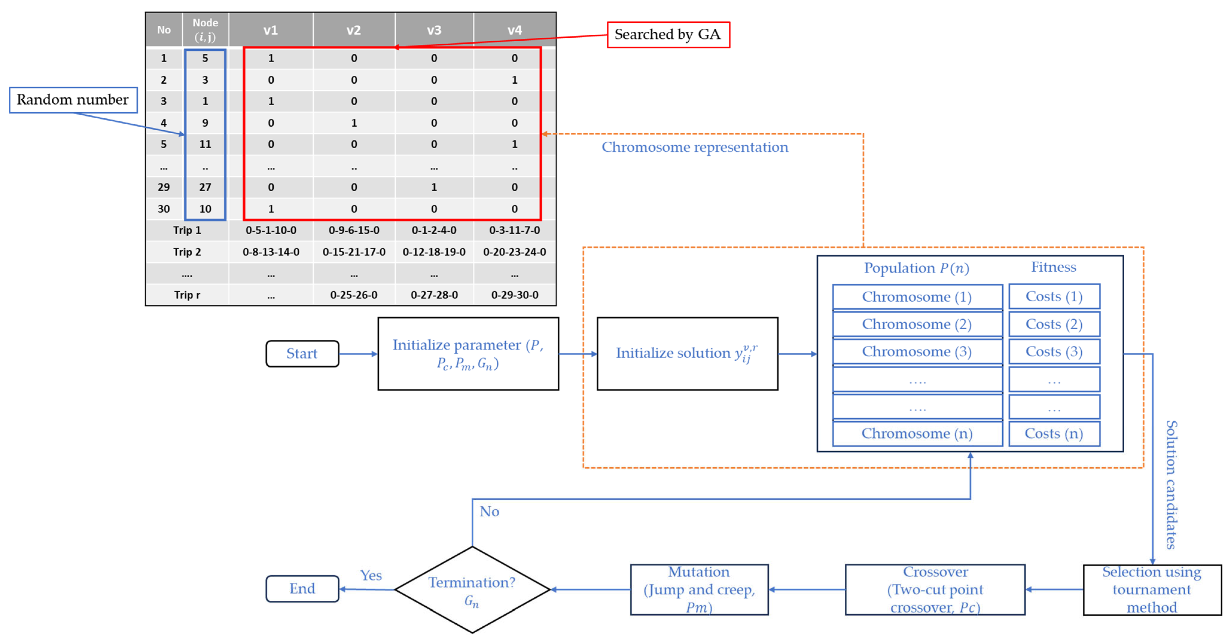
4.1. Population Initialization
4.2. Evaluate Fitness
4.3. Selection
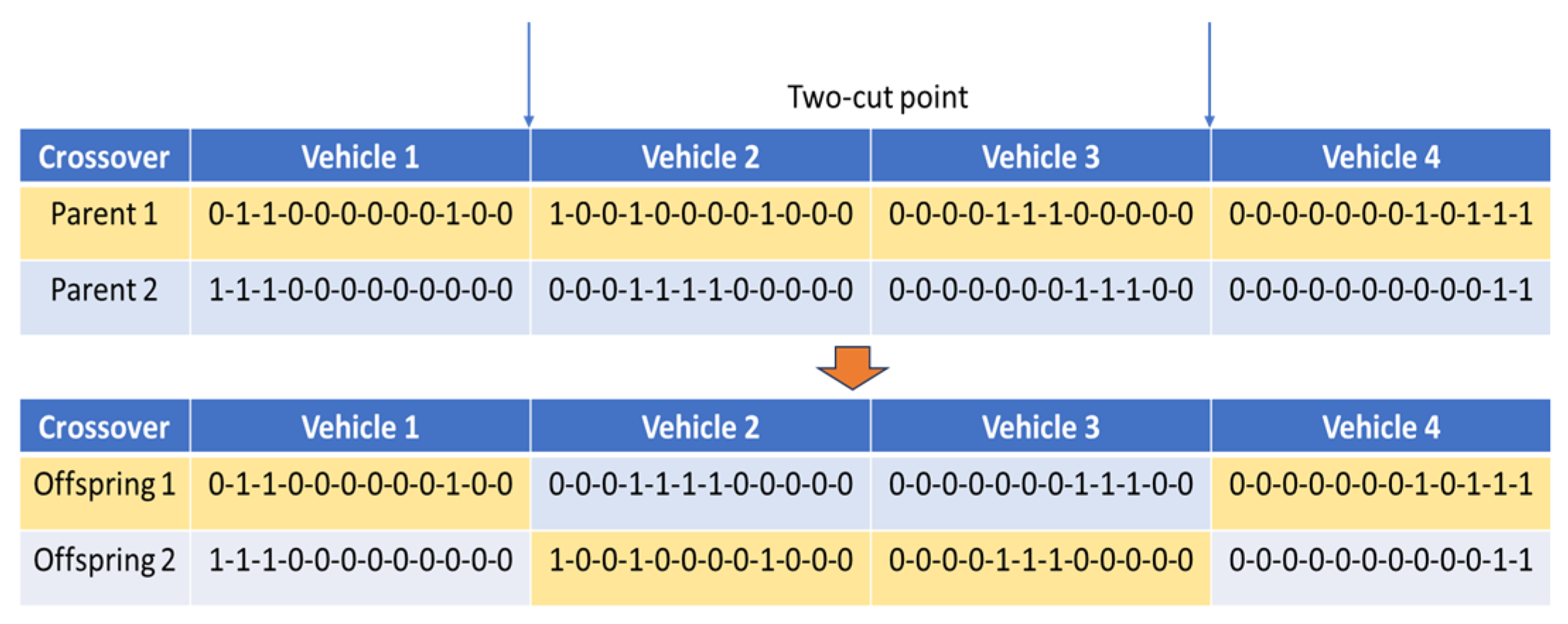
4.4. Crossover
4.5. Mutation
- Creep mutation: slightly adjusts the vehicle allocation or sequence in the chromosome, representing small, localized changes.
- Jump mutation: makes more considerable changes, such as reallocating a vehicle to a completely different route or swapping nodes between trips.
4.6. Evaluate Fitness Across Generations
5. Computational Experiment
5.1. Case Study
5.2. Model Evaluation
5.2.1. Parameter GA Tuning
- Combination 1: = 100, = 0.80, and = 0.025.
- Combination 2: = 125, = 0.65, and = 0.005.
- Combination 3: = 150, = 0.95, and = 0.001.
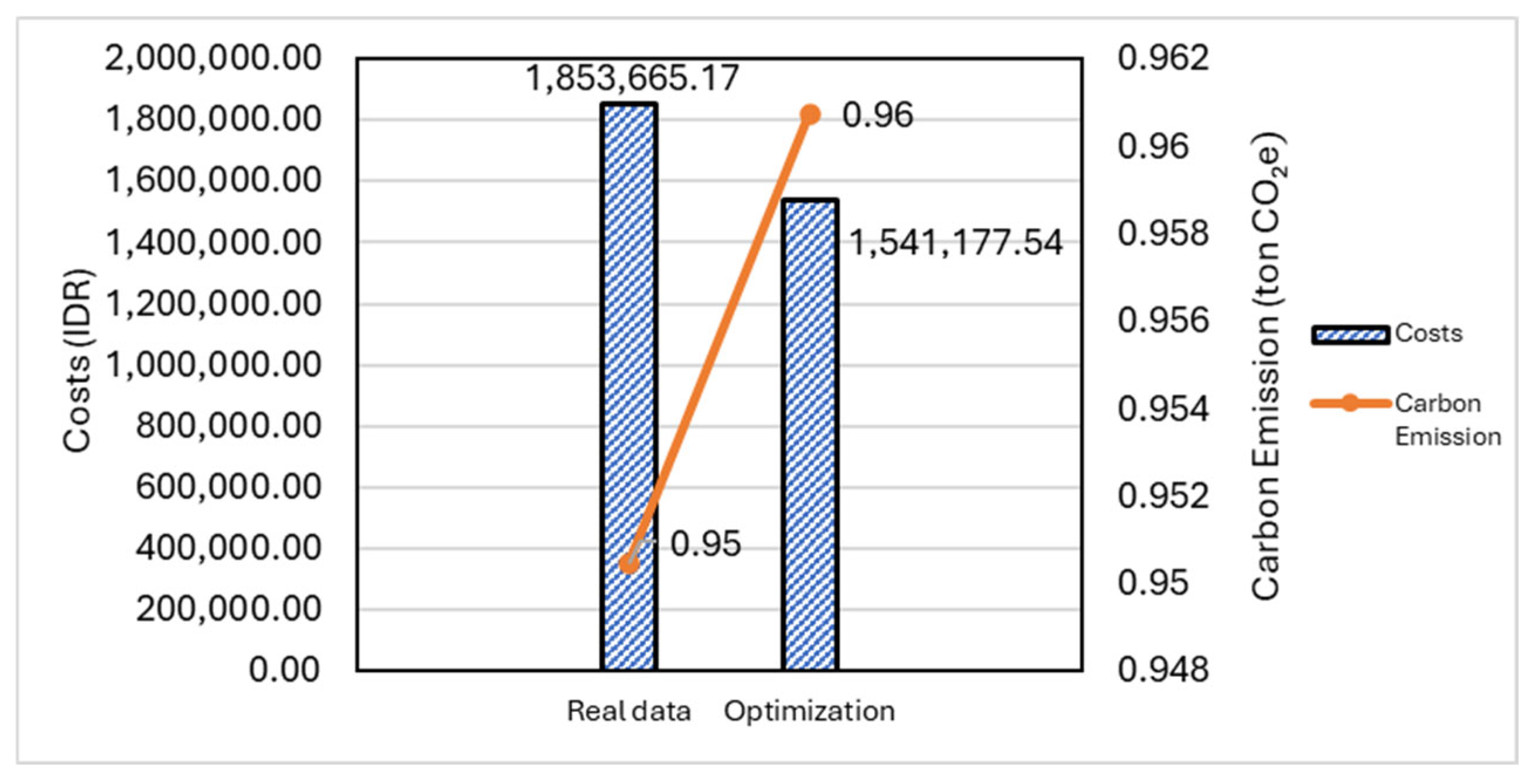
5.2.2. Performance Comparison of the Optimized Route Model with Actual Data Route
5.2.3. Sensitivity Analysis on Different Scenarios
6. Conclusions
Author Contributions
Funding
Institutional Review Board Statement
Informed Consent Statement
Data Availability Statement
Conflicts of Interest
References
- International Energy Agency Tracking Transport. Available online: https://www.iea.org/energy-system/transport (accessed on 15 October 2024).
- Coulombel, N.; Dablanc, L.; Gardrat, M.; Koning, M. The Environmental Social Cost of Urban Road Freight: Evidence from the Paris Region. Transp. Res. Part D Transp. Environ. 2018, 63, 514–532. [Google Scholar] [CrossRef]
- Karaduman, H.A.; Karaman-Akgül, A.; Çağlar, M.; Akbaş, H.E. The Relationship between Logistics Performance and Carbon Emissions: An Empirical Investigation on Balkan Countries. Int. J. Clim. Chang. Strateg. Manag. 2020, 12, 449–461. [Google Scholar] [CrossRef]
- Sar, K.; Ghadimi, P. A Systematic Literature Review of the Vehicle Routing Problem in Reverse Logistics Operations. Comput. Ind. Eng. 2023, 177, 109011. [Google Scholar] [CrossRef]
- Filemon Agung Dirjen Migas: Tata Kelola Distribusi Jadi Penyebab LPG 3 Kg Langka. Available online: https://industri.kontan.co.id/news/dirjen-migas-tata-kelola-distribusi-jadi-penyebab-lpg-3-kg-langka (accessed on 15 October 2024).
- Lehmann, J.; Winkenbach, M. A Matheuristic for the Two-Echelon Multi-Trip Vehicle Routing Problem with Mixed Pickup and Delivery Demand and Time Windows. Transp. Res. Part C Emerg. Technol. 2024, 160, 104522. [Google Scholar] [CrossRef]
- Xu, Z.; Elomri, A.; Pokharel, S.; Mutlu, F. A Model for Capacitated Green Vehicle Routing Problem with the Time-Varying Vehicle Speed and Soft Time Windows. Comput. Ind. Eng. 2019, 137, 106011. [Google Scholar] [CrossRef]
- Wei, X.; Xiao, Z.; Wang, Y. Solving the Vehicle Routing Problem with Time Windows Using Modified Rat Swarm Optimization Algorithm Based on Large Neighborhood Search. Mathematics 2024, 12, 1702. [Google Scholar] [CrossRef]
- Tan, S.; Yeh, W. The Vehicle Routing Problem: State-of-the-Art Classification and Review. Appl. Sci. 2021, 11, 10295. [Google Scholar] [CrossRef]
- Demir, E.; Bektas, T.; Laporte, G. A Review of Recent Research on Green Road Freight Transportation. Eur. J. Oper. Res. 2014, 237, 775–793. [Google Scholar] [CrossRef]
- Vieira, B.S.; Ribeiro, G.M.; Bahiense, L. Metaheuristics with Variable Diversity Control and Neighborhood Search for the Heterogeneous Site-Dependent Multi-Depot Multi-Trip Periodic Vehicle Routing Problem. Comput. Oper. Res. 2023, 153, 106189. [Google Scholar] [CrossRef]
- Wang, Z.; Wen, P. Optimization of a Low-Carbon Two-Echelon Heterogeneous-Fleet Vehicle Routing for Cold Chain Logistics under Mixed Time Window. Sustainability 2020, 12, 1967. [Google Scholar] [CrossRef]
- Sabet, S.; Farooq, B. Green Vehicle Routing Problem: State of the Art and Future Directions. IEEE Access 2022, 10, 101622–101642. [Google Scholar] [CrossRef]
- Sherif, S.U.; Asokan, P.; Sasikumar, P.; Mathiyazhagan, K.; Jerald, J. Integrated Optimization of Transportation, Inventory and Vehicle Routing with Simultaneous Pickup and Delivery in Two-Echelon Green Supply Chain Network. J. Clean. Prod. 2021, 287, 125434. [Google Scholar] [CrossRef]
- Nguyen, V.S.; Pham, Q.D.; Nguyen, T.H.; Bui, Q.T. Modeling and Solving a Multi-Trip Multi-Distribution Center Vehicle Routing Problem with Lower-Bound Capacity Constraints. Comput. Ind. Eng. 2022, 172, 108597. [Google Scholar] [CrossRef]
- Zhou, Z.; Ha, M.; Hu, H.; Ma, H. Half Open Multi-Depot Heterogeneous Vehicle Routing Problem for Hazardous Materials Transportation. Sustainability 2021, 13, 1262. [Google Scholar] [CrossRef]
- Govindan, K.; Jafarian, A.; Khodaverdi, R.; Devika, K. Two-Echelon Multiple-Vehicle Location-Routing Problem with Time Windows for Optimization of Sustainable Supply Chain Network of Perishable Food. Int. J. Prod. Econ. 2014, 152, 9–28. [Google Scholar] [CrossRef]
- Vyakarnam, S.; Jaykumar, G.; Cherukara, J.A. Design and Optimization of an Eco-Efficient Vehicle Routing Model for Heterogeneous Fleets and Multi Depot Systems. Procedia Comput. Sci. 2023, 230, 629–640. [Google Scholar] [CrossRef]
- Leuveano, R.A.C.; Asih, H.M.; Ridho, M.I.; Darmawan, D.A. Balancing Inventory Management: Genetic Algorithm Optimization for A Novel Dynamic Lot Sizing Model in Perishable Product Manufacturing. J. Robot. Control 2023, 4, 878–895. [Google Scholar] [CrossRef]
- Bektaş, T.; Laporte, G. The Pollution-Routing Problem. Transp. Res. Part B Methodol. 2011, 45, 1232–1250. [Google Scholar] [CrossRef]
- Zhang, H.; Huang, M.; Fu, Y.; Wang, X. Optimizing Speed of a Green Truckload Pickup and Delivery Routing Problem with Outsourcing: Heuristic and Exact Approaches. Comput. Ind. Eng. 2024, 198, 110736. [Google Scholar] [CrossRef]
- Kopfer, H.W.; Schönberger, J.; Kopfer, H. Reducing Greenhouse Gas Emissions of a Heterogeneous Vehicle Fleet. Flex. Serv. Manuf. J. 2014, 26, 221–248. [Google Scholar] [CrossRef]
- Wang, S.; Han, C.; Yu, Y.; Huang, M.; Sun, W.; Kaku, I. Reducing Carbon Emissions for the Vehicle Routing Problem by Utilizing Multiple Depots. Sustainability 2022, 14, 1. [Google Scholar] [CrossRef]
- Kim, H.W.; Joo, G.H.; Lee, D.H. Multi-Period Heterogeneous Vehicle Routing Considering Carbon Emission Trading. Int. J. Sustain. Transp. 2019, 13, 340–349. [Google Scholar] [CrossRef]
- Pak, Y.J.; Mun, K.H. A Practical Vehicle Routing Problem in Small and Medium Cities for Fuel Consumption Minimization. Clean. Logist. Supply Chain 2024, 12, 100164. [Google Scholar] [CrossRef]
- Gao, J.; Zheng, X.; Gao, F.; Tong, X.; Han, Q. Heterogeneous Multitype Fleet Green Vehicle Path Planning of Automated Guided Vehicle with Time Windows in Flexible Manufacturing System. Machines 2022, 10, 197. [Google Scholar] [CrossRef]
- Ren, X.; Huang, H.; Feng, S.; Liang, G. An Improved Variable Neighborhood Search for Bi-Objective Mixed-Energy Fleet Vehicle Routing Problem. J. Clean. Prod. 2020, 275, 124155. [Google Scholar] [CrossRef]
- Qiang, H.; Ou, R.; Hu, Y.; Wu, Z.; Zhang, X. Path Planning of an Electric Vehicle for Logistics Distribution Considering Carbon Emissions and Green Power Trading. Sustainability 2023, 15, 16045. [Google Scholar] [CrossRef]
- Liu, G.; Hu, J.; Yang, Y.; Xia, S.; Lim, M.K. Vehicle Routing Problem in Cold Chain Logistics: A Joint Distribution Model with Carbon Trading Mechanisms. Resour. Conserv. Recycl. 2020, 156, 104715. [Google Scholar] [CrossRef]
- Wen, M.; Sun, W.; Yu, Y.; Tang, J.; Ikou, K. An Adaptive Large Neighborhood Search for the Larger-Scale Multi Depot Green Vehicle Routing Problem with Time Windows. J. Clean. Prod. 2022, 374, 133916. [Google Scholar] [CrossRef]
- Su, Y.; Zhang, S.; Zhang, C. A Lightweight Genetic Algorithm with Variable Neighborhood Search for Multi-Depot Vehicle Routing Problem with Time Windows. Appl. Soft Comput. 2024, 161, 111789. [Google Scholar] [CrossRef]
- Qi, R.; Li, J.Q.; Wang, J.; Jin, H.; Han, Y.Y. QMOEA: A Q-Learning-Based Multiobjective Evolutionary Algorithm for Solving Time-Dependent Green Vehicle Routing Problems with Time Windows. Inf. Sci. 2022, 608, 178–201. [Google Scholar] [CrossRef]
- Chen, W.; Zhang, D.; Van Woensel, T.; Xu, G.; Guo, J. Green Vehicle Routing Using Mixed Fleets for Cold Chain Distribution. Expert Syst. Appl. 2023, 233, 120979. [Google Scholar] [CrossRef]
- Zhou, S.; Zhang, D.; Ji, B.; Zhou, S.; Li, S.; Zhou, L. A MILP Model and Heuristic Method for the Time-Dependent Electric Vehicle Routing and Scheduling Problem with Time Windows. J. Clean. Prod. 2024, 434, 140188. [Google Scholar] [CrossRef]
- Liu, Y.; Roberto, B.; Zhou, J.; Yu, Y.; Zhang, Y.; Sun, W. Efficient Feasibility Checks and an Adaptive Large Neighborhood Search Algorithm for the Time-Dependent Green Vehicle Routing Problem with Time Windows. Eur. J. Oper. Res. 2023, 310, 133–155. [Google Scholar] [CrossRef]
- Lou, P.; Zhou, Z.; Zeng, Y.; Fan, C. Vehicle Routing Problem with Time Windows and Carbon Emissions: A Case Study in Logistics Distribution. Environ. Sci. Pollut. Res. 2024, 31, 41600–41620. [Google Scholar] [CrossRef]
- Islam, M.A.; Gajpal, Y.; ElMekkawy, T.Y. Mixed Fleet Based Green Clustered Logistics Problem under Carbon Emission Cap. Sustain. Cities Soc. 2021, 72, 103074. [Google Scholar] [CrossRef]
- Islam, M.A.; Gajpal, Y. Optimization of Conventional and Green Vehicles Composition under Carbon Emission Cap. Sustainability 2021, 13, 6940. [Google Scholar] [CrossRef]
- Olgun, B.; Koç, Ç.; Altıparmak, F. A Hyper Heuristic for the Green Vehicle Routing Problem with Simultaneous Pickup and Delivery. Comput. Ind. Eng. 2021, 153, 107010. [Google Scholar] [CrossRef]
- Santos, M.J.; Jorge, D.; Ramos, T.; Barbosa-Póvoa, A. Green Reverse Logistics: Exploring the Vehicle Routing Problem with Deliveries and Pickups. Omega 2023, 118, 102864. [Google Scholar] [CrossRef]
- Zhao, J.; Dong, H.; Wang, N. Green Split Multiple-Commodity Pickup and Delivery Vehicle Routing Problem. Comput. Oper. Res. 2023, 159, 106318. [Google Scholar] [CrossRef]
- Xu, Z.; Ming, X.G.; Zheng, M.; Li, M.; He, L.; Song, W. Cross-Trained Workers Scheduling for Field Service Using Improved NSGA-II. Int. J. Prod. Res. 2015, 53, 1255–1272. [Google Scholar] [CrossRef]
- Chen, J.; Dan, B.; Shi, J. A Variable Neighborhood Search Approach for the Multi-Compartment Vehicle Routing Problem with Time Windows Considering Carbon Emission. J. Clean. Prod. 2020, 277, 123932. [Google Scholar] [CrossRef]
- Solomon, M.M. Algorithms for the Vehicle Routing and Scheduling Problems with Time Window Constraints. Oper. Res. 1987, 35, 254–265. [Google Scholar] [CrossRef]
- Gélinas, S.; Desrochers, M.; Desrosiers, J.; Solomon, M.M. A New Branching Strategy for Time Constrained Routing Problems with Application to Backhauling. Ann. Oper. Res. 1995, 61, 91–109. [Google Scholar] [CrossRef]
- Salhi, S.; Nagy, G. A Cluster Insertion Heuristic for Single and Multiple Depot Vehicle Routing Problems with Backhauling. J. Oper. Res. Soc. 1999, 50, 1034–1042. [Google Scholar] [CrossRef]
- Dethloff, J. Vehicle Routing and Reverse Logistics: The Vehicle Routing Problem with Simultaneous Delivery and Pick-Up. OR Spektrum 2001, 23, 79–96. [Google Scholar] [CrossRef]
- Hoff, A.; Gribkovskaia, I.; Laporte, G.; Løkketangen, A. Lasso Solution Strategies for the Vehicle Routing Problem with Pickups and Deliveries. Eur. J. Oper. Res. 2009, 192, 755–766. [Google Scholar] [CrossRef]
- Cordeau, J.F.; Laporte, G.; Mercier, A. Improved Tabu Search Algorithm for the Handling of Route Duration Constraints in Vehicle Routing Problems with Time Windows. J. Oper. Res. Soc. 2004, 55, 542–546. [Google Scholar] [CrossRef]
- Homberger, J.; Gehring, H. A Two-Phase Hybrid Metaheuristic for the Vehicle Routing Problem with Time Windows. Eur. J. Oper. Res. 2005, 162, 220–238. [Google Scholar] [CrossRef]
- Lu, J.; Chen, Y.; Hao, J.K.; He, R. The Time-Dependent Electric Vehicle Routing Problem: Model and Solution. Expert Syst. Appl. 2020, 161, 113593. [Google Scholar] [CrossRef]
- GHG Protocol Calculation Tools and Guidance. Available online: https://ghgprotocol.org/calculation-tools-and-guidance (accessed on 15 June 2024).
- Aghadavoudi Jolfaei, A.; Alinaghian, M. Multi-Depot Vehicle Routing Problem with Roaming Delivery Locations Considering Hard Time Windows: Solved by a Hybrid ELS-LNS Algorithm. Expert Syst. Appl. 2024, 255, 124608. [Google Scholar] [CrossRef]
- Zhao, W.; Bian, X.; Mei, X. An Adaptive Multi-Objective Genetic Algorithm for Solving Heterogeneous Green City Vehicle Routing Problem. Appl. Sci. 2024, 14, 6594. [Google Scholar] [CrossRef]
- Zhang, D.; Wang, X.; Li, S.; Ni, N.; Zhang, Z. Joint Optimization of Green Vehicle Scheduling and Routing Problem with Time-Varying Speeds. PLoS ONE 2018, 13, e0192000. [Google Scholar] [CrossRef] [PubMed]


| Authors | GVRP Characteristic | Decision Variables | Environmental Function | Model Objective | Model Solution | Case Study | ||||
|---|---|---|---|---|---|---|---|---|---|---|
| TW | HV | MT | SPD | VA | RP | |||||
| Kim et al. [24] | √ | √ | √ | CO2 emissions by distance; carbon trading | Min costs (travel and carbon trading) | Tabu search | Numerical example | |||
| Xu et al. [7] | √ | √ | Fuel-based vehicle load, capacity, and traffic conditions | Min fuel consumption; max customer satisfaction | Improved NSGA-II | Dataset from Xu et al. [42] | ||||
| Wang and Wen [12] | √ | √ | √ | √ | CO2 as a function of fuel and electricity consumption; carbon trading | Min costs, carbon emissions; max customer satisfaction | Adaptive Genetic Algorithm | Cold chain logistics | ||
| Liu et al. [29] | √ | √ | CO2 as a function of fuel, distance, vehicle load; carbon trading | Min costs (fixed, travel, damage, refrigeration, and emission) | SA | Cold chain logistics | ||||
| Chen et al. [43] | √ | √ | CO2 as a function of fuel and electricity consumption; carbon cost/tax | Min costs (fixed, travel, refrigeration, and emission) | VNS | Dataset from Solomon [44] | ||||
| Islam et al. [37] | √ | √ | √ | √ | √ | CO2 emissions by load, speed, and distance; emission cap | Min travel distance under emission constraint | Hybrid PSO and Neighborhood Search | Dataset from Gelinas et al. [45] | |
| Islam et al. [38] | √ | √ | √ | √ | CO2 emissions by fuel use, total weight, and distance | Min travel distance under emission constraint | Hybrid ACO and VNS | Dataset from Solomon [44] | ||
| Olgun et al. [39] | √ | √ | Fuel-based vehicle load and distance | Min fuel costs | Hyper-Heuristic algorithm | Dataset from [46]; Dethloff [47] | ||||
| Wen et al. [30] | √ | √ | CO2 emissions by fuel use | Min costs (carbon, fuel, vehicle rental, and driver salaries) | ALNS | Dataset from Solomon [44] | ||||
| Qi et al. [32] | √ | √ | CO2 emissions by fuel use | Min time duration vehicles and energy consumption; max customer satisfaction | QMOEA | Dataset from Solomon [44] | ||||
| Gao et al. [26] | √ | √ | √ | √ | Energy consumption-based distance | Min distance and energy | Hybrid GA- LNS | Dataset from Solomon [44] | ||
| Zhao et al. [41] | √ | √ | √ | CO2 emissions by distance | Min costs (transport, carbon, penalty, loading-unloading, and fuel consumption) | Two-stage search quantum PSO | Dataset from Solomon [44] | |||
| Liu et al. [35] | √ | √ | CO2 emissions by load, speed, and distance | Min carbon emissions | ALNS | Dataset from Solomon [44] | ||||
| Santos et al. [40] | √ | √ | CO2 emissions by fuel use | Min route costs; min emission | ALNS | Dataset from Hoff et al. [48] | ||||
| Chen et al. [33] | √ | √ | √ | √ | CO2 emissions by fuel; carbon prices | Min costs (fixed, energy consumption, damage, and carbon) | VNS | Cold supply chain | ||
| Su et al. [31] | √ | √ | CO2 emissions by fuel use | Min costs (distance; penalties, fuel; carbon emissions; and vehicle rental) | Hybrid GA and VNS | Dataset from Cordeau et al. [49]; Homberger and Gehring [50] | ||||
| Lou et al. [36] | √ | √ | CO2 emissions by fuel use and speed | Min carbon emissions | Hybrid GA and VNS | Logistic distribution, China | ||||
| Zhang et al. [21] | √ | √ | √ | CO2 emissions by fuel use | Min costs (fuel and outsource) | Heuristic algorithm | Numerical example of small–medium cities | |||
| Zhou et al. [34] | √ | √ | Energy consumption | Min costs (fixed, travel distance, and energy) | VNS with partial model (VNS-PM) | Lu et al. [51] | ||||
| Pak and Mun [25] | √ | √ | √ | √ | √ | Fuel consumption by speed | Min fuel consumption | VNS | Numerical example of small–medium cities | |
| This paper | √ | √ | √ | √ | √ | √ | CO2 emissions by vehicle load and distance; carbon tax | Min costs (travel, and carbon emission) | GA | LPG distribution |
| Notations | Descriptions |
|---|---|
| Sets and Indices | |
| Set of stations and depot, where 0 denotes the depot and 1, 2, 3, ..., are the stations (nodes). | |
| Set of vehicles, indexed as | |
| Indices for stations (nodes), where , ∈ M. | |
| Set of trips (or rounds) each vehicle can make, where represents individual trips by each vehicle. | |
| Parameters | |
| Number of full LPG cylinders delivered to station | |
| Number of empty LPG cylinders picked up from station (assumed for balance). | |
| Capacity of vehicle , in terms of the maximum number of LPG cylinders (full + empty) it can carry. | |
| Weight of a single full LPG cylinder. | |
| Weight of a single empty LPG cylinder. | |
| Tare weight (empty weight) of the vehicle at the depot. | |
| Total weight on vehicle v at station on trip , including both full and empty LPG cylinders. | |
| Distance between station and station , in kilometers. | |
| Average speed of single vehicle . | |
| Time window for station , with as the earliest and as the latest delivery times. | |
| Loading time per 10 units gallon of full LPG cylinders. | |
| Unloading time per 10 units gallon of full LPG cylinders. | |
| Loading time per 10 units gallon of empty LPG cylinders. | |
| Unloading time per 10 units gallon of empty LPG cylinders. | |
| Penalty cost per unit of time due to early arrivals. | |
| Penalty cost per unit of time due to late arrivals. | |
| Penalty cost per unit time for late returns to the depot. | |
| Cost per kilometer traveled. | |
| Arrival time of vehicle at station on trip . | |
| Vehicle returns to the depot after completing trip | |
| Total time for vehicle to complete all trips. | |
| Emission factor for CO2, in kgCO2/short ton-mile. | |
| Emission factor for CH₄, in gCH₄/short ton-mile. | |
| Emission factor for N2O, in gN2O/short ton-mile. | |
| Global Warming Potential for CO2. | |
| Global Warming Potential for CH₄. | |
| Global Warming Potential for N2O. | |
| Total CO2 equivalent emissions for vehicle traveling from station to station on trip , in ton CO2e. | |
| Carbon tax rate, representing the cost per ton of CO2e emitted. | |
| Variables | |
| Binary decision variable, where = 1 if vehicle is allocated to travel from station to station on trip , and = 0 otherwise. | |
| Conversion factors | |
| 0.621371: Conversion factor from kilometers (km) to miles. | |
| 0.00110231: Conversion factor from kilograms (kg) to short tons. | |
| 0.001: Conversion factor from grams to kilograms. | |
| Constraint | Descriptions |
|---|---|
| Objective model | Objective model (1) aims to minimize total operational costs, which include travel costs, carbon emission costs, and penalty costs incurred due to early or late arrivals. |
| Time-based penalties | Constraint Equation (2): A penalty is applied if a vehicle arrives at a station before its designated time window opens. |
| Constraint Equation (3): A penalty is applied for late arrivals after the time window closes. | |
| Constraint (4): A penalty is incurred if a vehicle returns to the depot later than the allowed time | |
| Vehicle capacity | Constraint (5) ensures that vehicles respect their capacity limits, accounting for the simultaneous transport of full cylinders for delivery and empty cylinders for pickup. |
| Station visits | Constraint (6) ensures that each station (excluding the depot) is visited exactly once, satisfying all its delivery and pickup demands. |
| Time window compliance | Constraint (7) enforces that station vehicle arrival times are within the specified time windows. |
| Arrival time calculations | Constraint (8a): Calculates arrival time from the depot to the first station, accounting for travel time, unloading full cylinders, and loading empty cylinders. |
| Constraint (8b): Calculates travel between two consecutive stations ( and ), considering the completion time at station , travel time, and operational times at station . | |
| Constraint (8c): Calculates travel time from the final station of the trip back to the depot, including unloading collected empty cylinders. | |
| Cumulative completion time | Constraint (9) ensures that the cumulative completion time of all trips is considered, including the final trip for each vehicle. |
| Vehicle weight management | Constraint (10): Defines the initial vehicle weight as the empty vehicle weight plus the load of full cylinders for delivery. |
| Constraint (11): Updates the vehicle’s weight dynamically after each delivery or pickup at a station | |
| Carbon Emissions Calculation based on GHG Protocol [52] | Constraints (12): Convert vehicle weight from kg to short tons. |
| Constraints (13): Convert distances from km to miles. | |
| Constraints (14–16): Convert CO2, CH₄, and N2O emissions into CO2 equivalents using Global Warming Potential (GWP). | |
| Constraint (17): Aggregate emissions for all trips into total CO2e (tons) to assess the environmental impact of the model. |
| Vehicle Type, | (Units) | (km/hr) | (IDR/km) |
|---|---|---|---|
| 1 | 560 | 50 | 1410 |
| 2 | 560 | 50 | |
| 3 | 360 | 55 | |
| 4 | 250 | 65 |
| Parameter | Value | Parameter | Value |
|---|---|---|---|
| IDR 5000/hour | 0.2970 kg CO2/short ton-mile | ||
| IDR 5000/hour | 0.0035 g CH₄/short ton-mile | ||
| IDR 10000/hour | 0.0027 g N2O/short ton-mile | ||
| 39.29 s/10 gallon | 1 | ||
| 32.56 s/10 gallon | 28 | ||
| 28.34 s/10 gallon | 265 | ||
| 24.45 s/10 gallon | 0.6213 | ||
| 8 kg/gallon | 0.0011 | ||
| 5 kg/gallon | 0.001 | ||
| IDR 30,000/ton CO2e |
| Fitness Function in IDR (Transportation Costs + Emission Costs + Penalty Costs) | |||||||
|---|---|---|---|---|---|---|---|
| Experiment | I | II | III | IV | V | Average | SD |
| Combination 1 | 1,641,025.40 | 1,702,377.38 | 1,766,129.97 | 1,572,360.49 | 1,700,177.97 | 1,676,414.24 | 73,087.73 |
| Combination 2 | 1,695,196.24 | 1,561,700.50 | 1,695,456.43 | 1,728,208.59 | 1,604,355.88 | 1,656,983.53 | 70,466.14 |
| Combination 3 | 1,553,785.04 | 1,613,426.07 | 1,541,177.54 | 1,665,997.19 | 1,601,173.77 | 1,595,111.92 | 50,034.25 |
| Difference of Levels | Difference of Means | SE of Difference | 95% CI | T-Value | Adjusted p-Value |
|---|---|---|---|---|---|
| Combination 2—Combination 1 | −19,431 | 41,329 | (−129,606; 90,744) | −0.47 | 0.886 |
| Combination 3—Combination 1 | −81,302 | 41,329 | (−191,477; 28,873) | −1.97 | 0.163 |
| Combination 3—Combination 2 | −61,872 | 41,329 | (−172,046; 48,303) | −1.50 | 0.327 |
| Trip | Route Planning | Capacity Usage (%) | Visualization | ||
|---|---|---|---|---|---|
| 1 | Trip 1 Trip 2 Trip 3 | 071878204767180 060392823048620 0508118384410 | 82.70 74.40 53.10 | 92.86 83.93 96,43 |  |
| 2 | Trip 1 Trip 2 Trip 3 Trip 4 Trip 5 Trip 6 Trip 7 | 0566496553850 0733838254220 07743324286750 0737341968140 049583324800 06945784 8825790 0291066175760 | 103.90 53.00 90.80 68.80 42.90 99.70 49.90 | 91.07 87.50 96,43 75,00 85,71 98,21 76,79 |  |
| 3 | Trip 1 Trip 2 Trip 3 Trip 4 Trip 5 Trip 6 | 02670760 0213627150 0441223550 0727461160 0515211630 05350 | 34.40 30.20 66.80 51.20 48.20 44.30 | 86,11 86,11 88,89 86,11 75,00 63,89 |  |
| 4 | Trip 1 Trip 2 | 03159460 040130 | 58.70 12.50 | 92,00 88,00 | 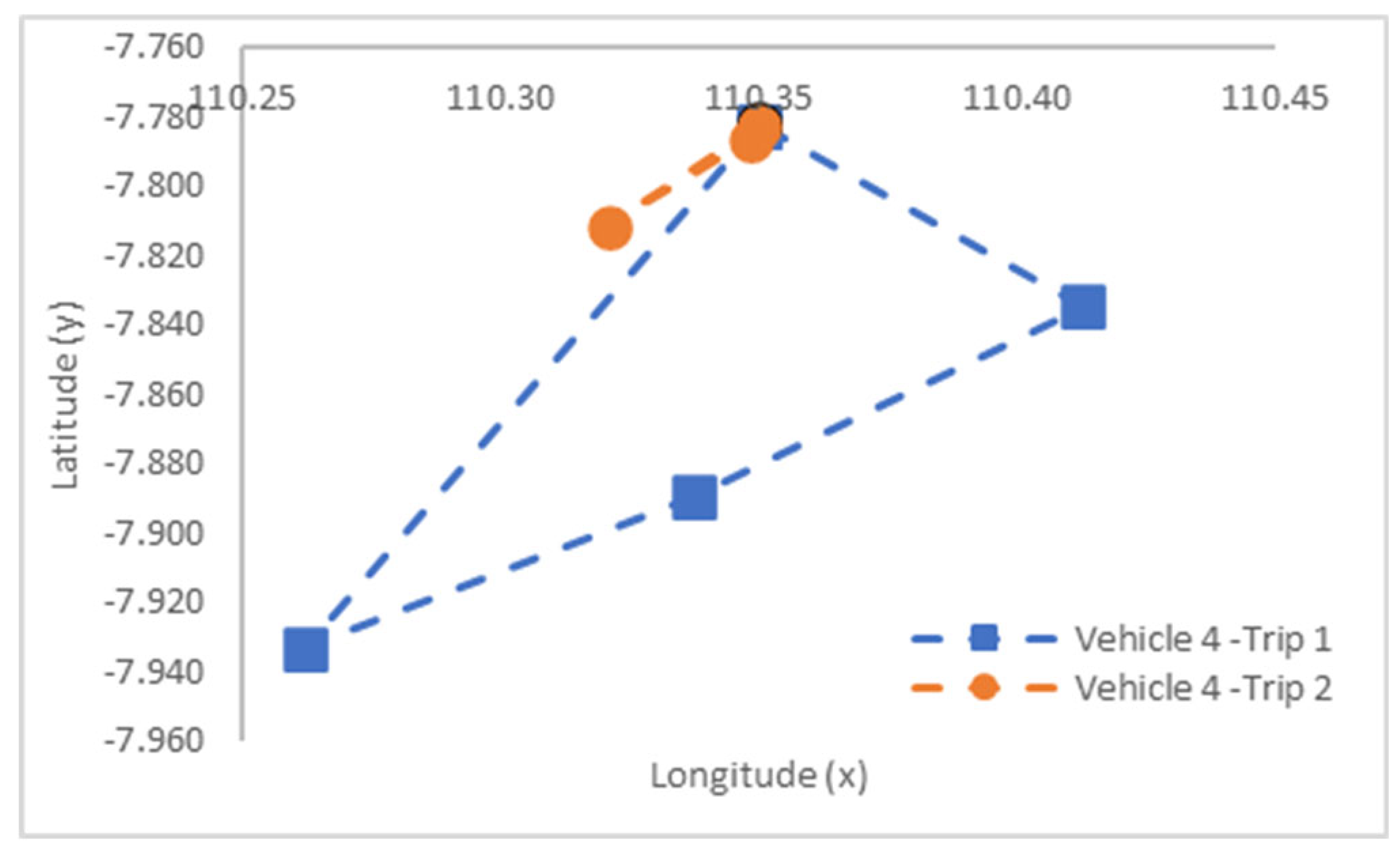 |
| Vehicle | Trip | Time | Status | Penalty Costs (IDR) | Total Distance | Delivery Unit | Total Costs (IDR) | Emissions (Ton CO2e) |
|---|---|---|---|---|---|---|---|---|
| Vehicle 1 | Trip—1 | 11:01 | Start | 0.00 | 82.70 | 520.00 | 116,607.00 | 0.08 |
| Trip—2 | 14:05 | Continue | 0.00 | 74.40 | 470.00 | 104,904.00 | 0.06 | |
| Trip—3 | 16:55 | Continue | 0.00 | 53.10 | 540.00 | 74,871.00 | 0.05 | |
| Total | 0.00 | 210.20 | 296,382.00 | 0.20 | ||||
| Vehicle 2 | Trip—1 | 11:25 | Start | 0.00 | 103.90 | 510.00 | 146,499.00 | 0.11 |
| Trip—2 | 14:09 | Continue | 0.00 | 53.00 | 490.00 | 74,730.00 | 0.05 | |
| Trip—3 | 17:44 | Continue | 0.00 | 90.80 | 540.00 | 128,028.00 | 0.10 | |
| Trip—4 | 10:50 | Start | 0.00 | 68.80 | 420.00 | 97,008.00 | 0.06 | |
| Trip—5 | 13:16 | Continue | 0.00 | 42.90 | 480.00 | 60,489.00 | 0.04 | |
| Trip—6 | 17:03 | Continue | 0.00 | 99.70 | 550.00 | 140,577.00 | 0.10 | |
| Trip—7 | 10:31 | Start | 0.00 | 49.90 | 430.00 | 70,359.00 | 0.05 | |
| Total | 0.00 | 509.00 | 717,690.00 | 0.51 | ||||
| Vehicle 3 | Trip—1 | 09:27 | Start | 10,000.00 | 34.40 | 310.00 | 48,504.00 | 0.03 |
| Trip—2 | 11:03 | Continue | 0.00 | 30.20 | 310.00 | 42,582.00 | 0.03 | |
| Trip—3 | 13:20 | Continue | 0.00 | 66.80 | 320.00 | 94,188.00 | 0.05 | |
| Trip—4 | 15:19 | Continue | 0.00 | 51.20 | 310.00 | 72,192.00 | 0.04 | |
| Trip—5 | 17:07 | Continue | 0.00 | 48.20 | 270.00 | 67,962.00 | 0.04 | |
| Trip—6 | 09:36 | Start | 0.00 | 44.30 | 230.00 | 62,463.00 | 0.03 | |
| Total | 10,000.00 | 275.10 | 387,891.00 | 0.21 | ||||
| Vehicle 4 | Trip—1 | 09:30 | Start | 0.00 | 58.70 | 230.00 | 82,767.00 | 0.03 |
| Trip—2 | 10:26 | Continue | 0.00 | 12.50 | 220.00 | 17,625.00 | 0.01 | |
| Total | 10:26 | 0.00 | 71.20 | 100,392.00 | 0.04 |
| Vehicle | Trip | Route Planning | Total Distance (km) | Delivery Unit | Total Costs (IDR) | Emissions (Ton CO2e) | Emission Costs (IDR) |
|---|---|---|---|---|---|---|---|
| 1 | 1 | 056538570760 | 71.10 | 460 | 375,550.28 | 0.26 | 7681.28 |
| 2 | 1 2 | 071649318200 07338382210 | 143.10 | 530 450 | |||
| 3 | 1 | 0266587590 | 46.70 | 320 |
| Vehicle | Trip | Route Planning | Total Distance (km) | Delivery unit | Total Costs (IDR) | Emissions (Ton CO2e) | Emission Costs (IDR) |
|---|---|---|---|---|---|---|---|
| 1 | 1 2 | 071318204767180 07744757370 | 112.90 | 530 410 | 647,195.22 | 0.42 | 12,554.22 |
| 2 | 1 2 | 06487857073380 038222433212230 | 169.70 | 550 510 | |||
| 3 | 1 2 3 | 056926650 0535976270 06042860 | 132.00 | 350 350 290 | |||
| 4 | 1 2 | 021540 036150 | 35.50 | 230 90 |
| Vehicle | Trip | Route Planning | Total Distance (km) | Delivery Unit | Total Costs (IDR) | Emissions (Ton CO2e) | Emission Costs (IDR) |
|---|---|---|---|---|---|---|---|
| 1 | 1 | 064987859760 0773734195152800 | 138.80 | 510 560 | 1,024,945.40 | 0.65 | 19,490.90 |
| 2 | 1 2 3 4 5 | 05626655385700 0733838221540 0362767184332600 042556839282580 0332430480 | 338.75 | 540 560 530 560 300 | |||
| 3 | 1 2 3 | 071312047150 04412752370 014727461160 | 167.60 | 350 350 360 | |||
| 4 | 1 2 | 022860 0490 | 57.30 | 170 150 |
Disclaimer/Publisher’s Note: The statements, opinions and data contained in all publications are solely those of the individual author(s) and contributor(s) and not of MDPI and/or the editor(s). MDPI and/or the editor(s) disclaim responsibility for any injury to people or property resulting from any ideas, methods, instructions or products referred to in the content. |
© 2025 by the authors. Licensee MDPI, Basel, Switzerland. This article is an open access article distributed under the terms and conditions of the Creative Commons Attribution (CC BY) license (https://creativecommons.org/licenses/by/4.0/).
Share and Cite
Indrianti, N.; Leuveano, R.A.C.; Abdul-Rashid, S.H.; Ridho, M.I. Green Vehicle Routing Problem Optimization for LPG Distribution: Genetic Algorithms for Complex Constraints and Emission Reduction. Sustainability 2025, 17, 1144. https://doi.org/10.3390/su17031144
Indrianti N, Leuveano RAC, Abdul-Rashid SH, Ridho MI. Green Vehicle Routing Problem Optimization for LPG Distribution: Genetic Algorithms for Complex Constraints and Emission Reduction. Sustainability. 2025; 17(3):1144. https://doi.org/10.3390/su17031144
Chicago/Turabian StyleIndrianti, Nur, Raden Achmad Chairdino Leuveano, Salwa Hanim Abdul-Rashid, and Muhammad Ihsan Ridho. 2025. "Green Vehicle Routing Problem Optimization for LPG Distribution: Genetic Algorithms for Complex Constraints and Emission Reduction" Sustainability 17, no. 3: 1144. https://doi.org/10.3390/su17031144
APA StyleIndrianti, N., Leuveano, R. A. C., Abdul-Rashid, S. H., & Ridho, M. I. (2025). Green Vehicle Routing Problem Optimization for LPG Distribution: Genetic Algorithms for Complex Constraints and Emission Reduction. Sustainability, 17(3), 1144. https://doi.org/10.3390/su17031144