Parametric Analysis of the Factors Impacting the Spatial Distribution of Particles in a Bus Environment

Abstract

This study presents a parametric analysis of the factors impacting particle distribution within a bus environment using computational fluid dynamics (CFD) simulations, with a primary focus on the relative concentration (RC) of particles. The Novel Relative Concentration (RC) metric, which measures the deviation from a return concentration, was used to assess the effects of ventilation rates, the number and spatial arrangement of particle emitters, and thermal conditions. Our investigation reveals that increasing air changes per hour (ACHs) from 5.74 h⁻¹ to 28.66 h⁻¹ reduces the overall particle concentration by approximately 45%, but localized high concentration zones persist, with maximum RC values observed at 1.57. Scenarios with evenly distributed emitters achieved near-uniform particle distribution, with RC values averaging around 0.95, while clustered emitters resulted in localized high concentrations, with RC values exceeding 2.0. Thermal conditions were found to have a minimal effect on RC, with average values of 1.664 for cooling and 1.588 for heating, showing only a 4.68% difference. The RC metric provided clear insights into the non-uniformity of particle distribution, highlighting areas prone to higher concentrations, with some zones reaching RC values of 2.5, indicating concentrations 2.5 times higher than the well-mixed average. These findings underscore the importance of optimizing ventilation systems for both overall air exchange and uniform air distribution, offering practical implications for improving air quality and reducing the risk of airborne pathogen transmission in public transportation systems. Future research should explore real-time ventilation adjustments based on passenger load, the effects of different particle types, and the development of models incorporating human behavior and movement patterns.

1. Introduction

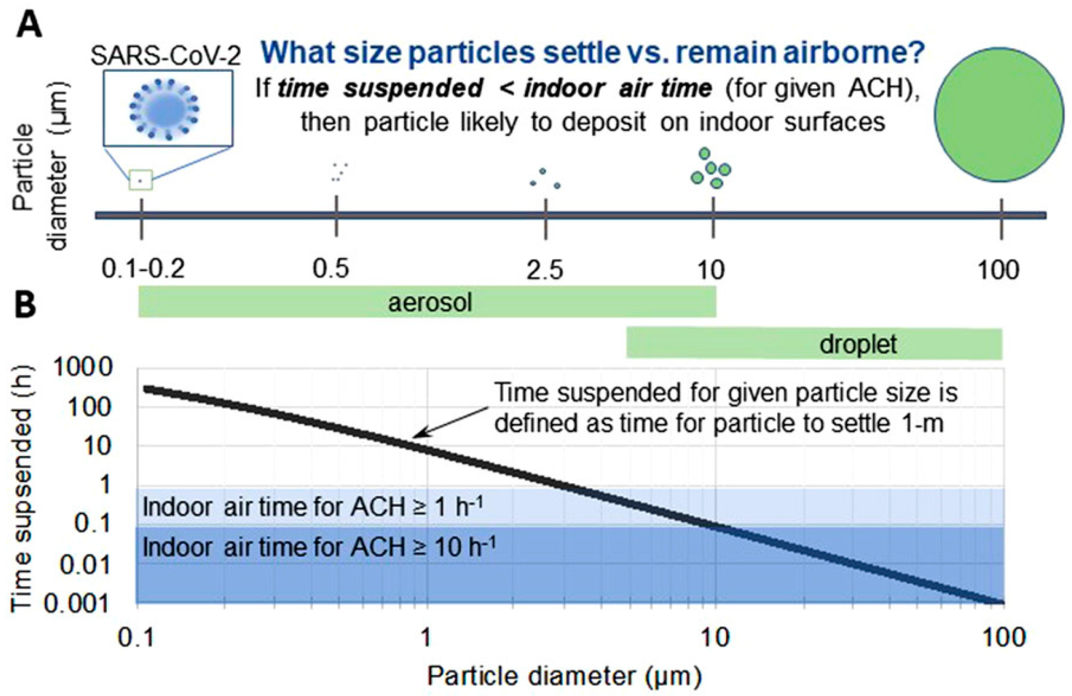
The predominant route of transmission is the inhalation of airborne particles/droplets containing infectious SARS-CoV-2 that are suspended in the air. Hence, understanding the transport behavior of airborne virus-laden particles is crucial for understanding transmission dynamics. Indoor particle transport can be divided into two specific mechanisms based on particle size [1]. Large particles tend to fall out of the air and are not impacted by spatial airflow, while small particles tend to be carried away by airflow and hence have greater potential for infection over distance. The spectrum of particle sizes is often grouped into three separate categories: ultrafine particles (0.1 µm or less), fine particles (0.1 µm to 2.5 µm), or coarse particles (>2.5 μm) [2]. A particle that is larger than 10 µm may fall out of airflow streams and settle on or impact surfaces, while a particle that is smaller will remain suspended in air and continue to be carried by airflow (Figure 1). Particle sizes, however, can change over time, especially for larger droplets. It has been shown that since droplets are mostly made up of water, their evaporation kinetics are determined by conditions such as relative humidity, air temperature, and velocity. As they rapidly evaporate, they produce different sizes of aerosols that can alter their behaviors over time [3].

Consequently, the quantity and size distribution of particles emitted by aerosol or droplet-generating expiratory actions must be considered, along with the velocity of the generating or initial carrying event that influences particle transport (droplets in particular) [4]. A number of actions are associated with the generation of aerosols and/or droplets, such as breathing, talking, coughing, and sneezing, but aerosol generation is not uniform, with a high degree of variability between individuals [5,6,7]. Sneezing and coughing can also generate high initial velocity [8], but the impact of the initial airflow field dissipates within one meter of the mouth [9]. Some of these initial sneezing droplets have diameters of tens or hundreds of µm [10], but there is substantial variation across test subjects. When people breathe, talk, or cough, they produce particle sizes varying from 0.1 µm to 10 µm for breathing, 0.05 µm to 10 µm for talking, and 0.05 µm to 5 µm for coughing [11].

The size of viable SARS-CoV-2-laden aerosol particles has been determined mainly using the viral RNA of the virus, which has been detected in aerosols with a diameter of >1 μm, with the majority of RNA detected in aerosols larger than 4 μm in hospitals undergoing COVID-19 outbreaks [12]. Hence, it is reasonable to consider the minimum airborne particles of size 1 μm as the primary viable virus-carrying aerosolized particle size when modeling airborne transport behavior.

Bulk airflow within the indoor environment is influenced by two factors; the first is the natural convection contributed by thermal buoyancy from the heat generated from indoor equipment and occupants; the second is the movement of forced air produced by the heating, ventilation, and air-conditioning (HVAC) system. These mechanisms significantly increase the distance to which exhaled particles can spread indoors [13,14]. Due to the recirculation of airborne droplets in HVAC systems, aerosolized droplets can travel to the entire HVAC zone or building, although their concentrations are significantly diminished by dilution and filtration [15]. However, ref. [16] documents that SARS-CoV-2 transmission is often associated with localized airflow without proper dilution and filtration, which highlights the importance of establishing local airflow patterns that prevent indoor COVID-19 transmission.

While indoor particle dynamics modeling is well established and extensively researched for various environments such as offices, classrooms, aircraft cabins, and hospitals, it remains relatively scarce in the context of public transit settings. In public transit, much of the available literature relies heavily on field observations. These previous investigations typically focus on assessing the impact of factors like ventilation and vehicle exhaust on air quality inside buses [17,18,19]. In the case of subway systems, investigations have traditionally centered on documenting elevated particle concentrations, often in the hundreds of micrograms per cubic meter range, particularly in underground stations and tunnels. These particles are primarily derived from mechanical processes associated with braking on train cars [20,21,22,23].

Most model-based studies related to public transit particle concentrations have relied on semi-empirical statistical frameworks or machine learning algorithms to predict in-cabin air quality based on ambient environmental data. These approaches are favored over using physics-based models simulating in-cabin concentrations for certain applications considering exposure to pollutants like diesel exhaust [24,25,26,27]. However, since the onset of the COVID-19 pandemic, investigations using Quantitative Microbial Risk Assessment (QMRA) or Wells–Riley risk models have started to incorporate parameters relevant to public transit settings, albeit partially. For instance, ref. [28] employed a risk model to estimate the probabilities of SARS-CoV-2 infection within various settings, including buses, classrooms, aircraft cabins, and offices. They considered factors such as spatial volume, exposure time, and ventilation rate specific to each environment. Similarly, ref. [29] developed infection probability models based on exposure time for a range of settings, including restaurants, classrooms, offices, high-speed rail cabins, subway cars, long-distance buses, public transit buses, and aircraft cabins. They distinguished these environments based on cabin dimensions, occupancy, occupant proximity, and ventilation rates.

With different particle sizes and different initial velocities, the fate of exhaled particles is difficult to determine. Furthermore, none of the above studies considered ventilation air distribution, the orientation of the occupants, and specific airflow-driven infection paths inside the cabin space. These shortcomings demonstrate the potentially significant spatial discrepancy in terms of particle concentration and the associated risks in a given space that is typically modeled based on a well-mixed assumption where pollutant concentration is homogenous within the investigation space. The well-mixed assumption is based on the idea that turbulent airflow in indoor spaces promotes the effective mixing of airborne pollutants. However, it is acknowledged that turbulence can sometimes cause uneven distribution of particles, although this is expected to be less significant for smaller particles [30]. Achieving a perfect well-mixed state in an indoor space is considered unlikely under practical ventilation conditions. The limitations of the well-mixed assumption are recognized, especially in cases where a receiver is directly in the flow path of an infected person’s exhalation, leading to higher pathogen concentrations than the average well-mixed assumption suggests [31]. Conversely, there are instances where pathogen concentrations might be lower than the well-mixed assumption predicts, making the average guideline overly restrictive. The well-mixed assumption is further evaluated across different scenarios, considering variations in emitter and receiver locations within a room. Despite its simplicity and widespread use, the well-mixed approach may not accurately capture all aspects of airflow dynamics [32,33,34,35]. In addition, the well-mixed assumption has also been investigated in relation to the cooling and heating of indoor spaces [36]. The well-mixed model remains fundamental but incorporating correction factors can enhance its accuracy by accounting for emitter location and other important variables.

While the literature on the transmission and distribution of particles in buildings and the effect of building ventilation is widely studied, specific studies relating to infectious aerosols in mass transit environments are scarce. Hence, this work focuses on particle transport and distribution within a public transit bus environment to understand whether spatial variances in particle concentration could impact analyses typically based on the well-mixed assumption. Furthermore, this work can improve sustainability for the urban environment by helping public transportation operators to manage ridership health more efficiently and providing tools to improve IAQ in the vehicles while minimizing energy expenditure.

2. Methodology

The present work utilizes computational fluid dynamics (CFD) simulations to investigate the spatial distribution of particles in a typical mass transit bus operated by the Southeastern Pennsylvania Transportation Authority (SEPTA), the partner organization of this investigation. Various ventilation rate and occupant emission scenarios were examined to better understand their relationship with disease transmission probabilities in an effort to aid investigators, engineers, and transit agencies in determining strategies to protect riders and operators during times of high community levels of an infectious disease. Below is a detailed description of the CFD-based investigation methods, followed by key observations of the results and discussions.

2.1. Investigation Concept and Metric

While most of the current infection risk models have assumed a well-mixed scenario where indoor concentrations of pollutants/infectious agents are uniform, it is not clear whether such an approach would overestimate or underestimate the risk. Hence, this investigation simulated a bus cabin under different ventilation rates and ventilation modes to determine the following: (1) when, if ever, the well-mixed assumption is suitable; (2) how the ventilation rate impacts local pollutant concentrations; and (3) whether the rider seating arrangement impacts local concentrations.

To simplify the computational effort of this investigation, all particles are set to have 1 µm diameters for all simulations herein. Such a particle size has been established by previous works as being adequately representative of infectious aerosols. Because different emission and ventilation scenarios produce widely different particle concentrations, the absolute concentration is a poor metric for comparing the spatial distribution of particles between cases. Instead, a relative concentration (RC) concept is used by simply normalizing the local concentration of particles by the well-mixed concentration. This concept is similar to the ASHRAE Standard 129 [37] “Measuring Air-Change Effectiveness” method and is the reciprocal of the ASHRAE Standard 62.1’s [38] Zone Air Distribution Effectiveness (Ez) value. The relative concentration (RC) is determined by dividing the local concentration of particles by the well-mixed concentration. Mathematically, this is expressed as follows:

$$\mathrm{R}\mathrm{e}\mathrm{l}\mathrm{a}\mathrm{t}\mathrm{i}\mathrm{v}\mathrm{e} \mathrm{C}\mathrm{o}\mathrm{n}\mathrm{c}\mathrm{e}\mathrm{n}\mathrm{t}\mathrm{r}\mathrm{a}\mathrm{t}\mathrm{i}\mathrm{o}\mathrm{n}\left(\mathrm{R}\mathrm{C}\right)={\displaystyle \frac{\mathrm{L}\mathrm{o}\mathrm{c}\mathrm{a}\mathrm{l} \mathrm{C}\mathrm{o}\mathrm{n}\mathrm{c}\mathrm{e}\mathrm{n}\mathrm{t}\mathrm{r}\mathrm{a}\mathrm{t}\mathrm{i}\mathrm{o}\mathrm{n}}{\mathrm{w}\mathrm{e}\mathrm{l}\mathrm{l}-\mathrm{m}\mathrm{i}\mathrm{x}\mathrm{e}\mathrm{d} \mathrm{C}\mathrm{o}\mathrm{n}\mathrm{c}\mathrm{e}\mathrm{n}\mathrm{t}\mathrm{r}\mathrm{a}\mathrm{t}\mathrm{i}\mathrm{o}\mathrm{n}}}$$

In this CFD-based study, the well-mixed concentration is defined as the average concentration in the return area of the HVAC system. This practice is well adopted in CFD investigations due to the discrepancy between the theoretical well-mixed value and the reality of non-uniform mixing. The local concentration is calculated based a specific breathing volume around each rider’s head, defined in Section 2.6.

The RC values in this study indicate particle distribution: RC = 1 signifies well-mixed particles, RC < 1 implies less uniform mixing, and RC > 1 suggests a more concentrated and uneven distribution. For example, an RC of 0.1 represents a concentration 10 times less than well mixed, while an RC of 10 signifies a concentration 10 times greater. With the use of RC, different emission scenarios can be compared in terms of how well evenly or heterogeneously the particles are distributed. In this work, RC is defined as a metric used to assess and compare the distribution or dispersion of particles in the bus environment.

It is also important to note that the supply air is assumed to be 100% contaminant-free in this study. Buses typically only have recirculated ventilation and rely on open doors and other openings for fresh air. Realistically, the recirculated system will return some contaminants back into the cabin. However, with the key investigative metric, RC, not largely impacted by this additional concentration as it is a normalized ratio between local concentration and well-mixed concentration, using the assumption of 100% clean supply air can simplify the need to track particle concentration during recirculation.

Also, in this study, steady-state conditions have been used for analyzing the spatial distribution of particles inside the bus because the primary objective is to understand the long-term average distribution patterns rather than transient, time-varying behaviors. This approach is appropriate as the ventilation and airflow systems inside the bus operate under steady and continuous conditions during normal operations, ensuring that the equilibrium distribution of particles is accurately represented. By focusing on steady-state conditions, we can concentrate on the spatial distribution of particles without the added complexity of temporal variations. Additionally, steady-state simulations are computationally efficient compared to transient simulations, as they do not require us to track particle behavior over multiple time steps. This efficiency is particularly important when the goal is to achieve equilibrium results. Moreover, steady-state spatial distribution provides insights into persistent exposure levels that passengers may face during a typical journey, making it highly relevant to practical scenarios such as assessing air quality and contamination risks.

2.2. Investigation Scenarios

Urban rapid transit buses make frequent stops where factors like passenger movement and door openings influence the air exchange rate and spatial distribution of particles. But between stops, passengers are relatively stationary, and the ventilation is steady, resulting in a more stable environment that does not significantly alter the characteristics of the onboard air. Due to the complexities of the confounding factors during dwell times at bus stops, and because buses in service spend considerably more time between stops than they do when they are stopped with their doors open, this study focuses on the steady scenario between stops.

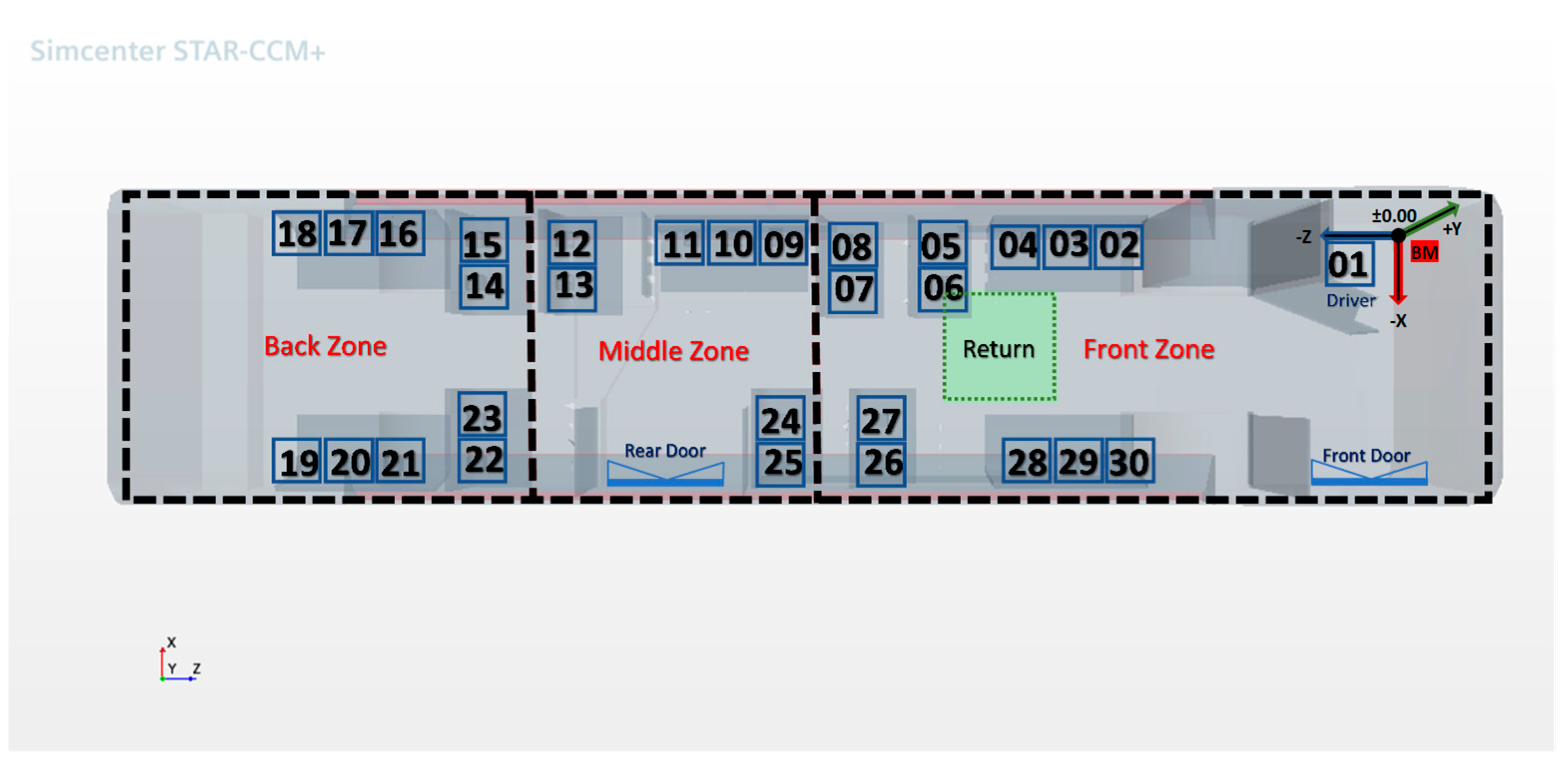
This study utilizes a Ney Flyer Xcelsior 40’ SEPTA bus model (one of the primary vehicles operated by the study partner SEPTA). Its approximate dimensions are 14 m in length, 2.6 m in width, and 3 m in height. This bus model serves as the basis for exploring how various scenarios and particle distributions affect the interior environment. The bus environment is shown in Figure 2, with additional descriptions summarized in

Table 1. Scenario simulations.

Varied Parameter	Scenarios	Simulations	Purpose
Thermal	Heating: inlet 90 °F, windows 50 °F Cooling: inlet 50 °F, windows 90 °F	2	Identify the distribution of particles in the bus. Analyze the relationship between the relative concentrations and thermal scenarios.
Air Change Per Hour ACH (λ)	Different velocity inlet: 0.1; 0.2; 0.3; 0.4; 0.5 m/s Equivalent ACH: 5.74; 11.47; 17.20; 22.93; 28.66 h−1	5	Analyze the distribution of particles in the bus. Examine the relationship between the relative concentration and different air exchange rates.
Number of Emitter/s	1, 5, 10	3	Investigate the distribution of particles in the bus and the relationship between the relative concentration and different numbers of emitters.
Location of Emitter/s	Front; Middle; Back; Distributed	3 + 1	Examine the distribution of particles and determine the relationship between the relative concentration and the location of different emitters.

. These buses do not provide dedicated outdoor air ventilation, but onboard air is recirculated and passed through a MERV 13 filter where it may also be thermally conditioned. Air supply openings are distributed lengthwise along both the upper-left and upper-right edges of the vehicle, while the return air outlet is positioned in the middle of the ceiling’s front section. Outdoor air infiltration was negligible in the following simulations.

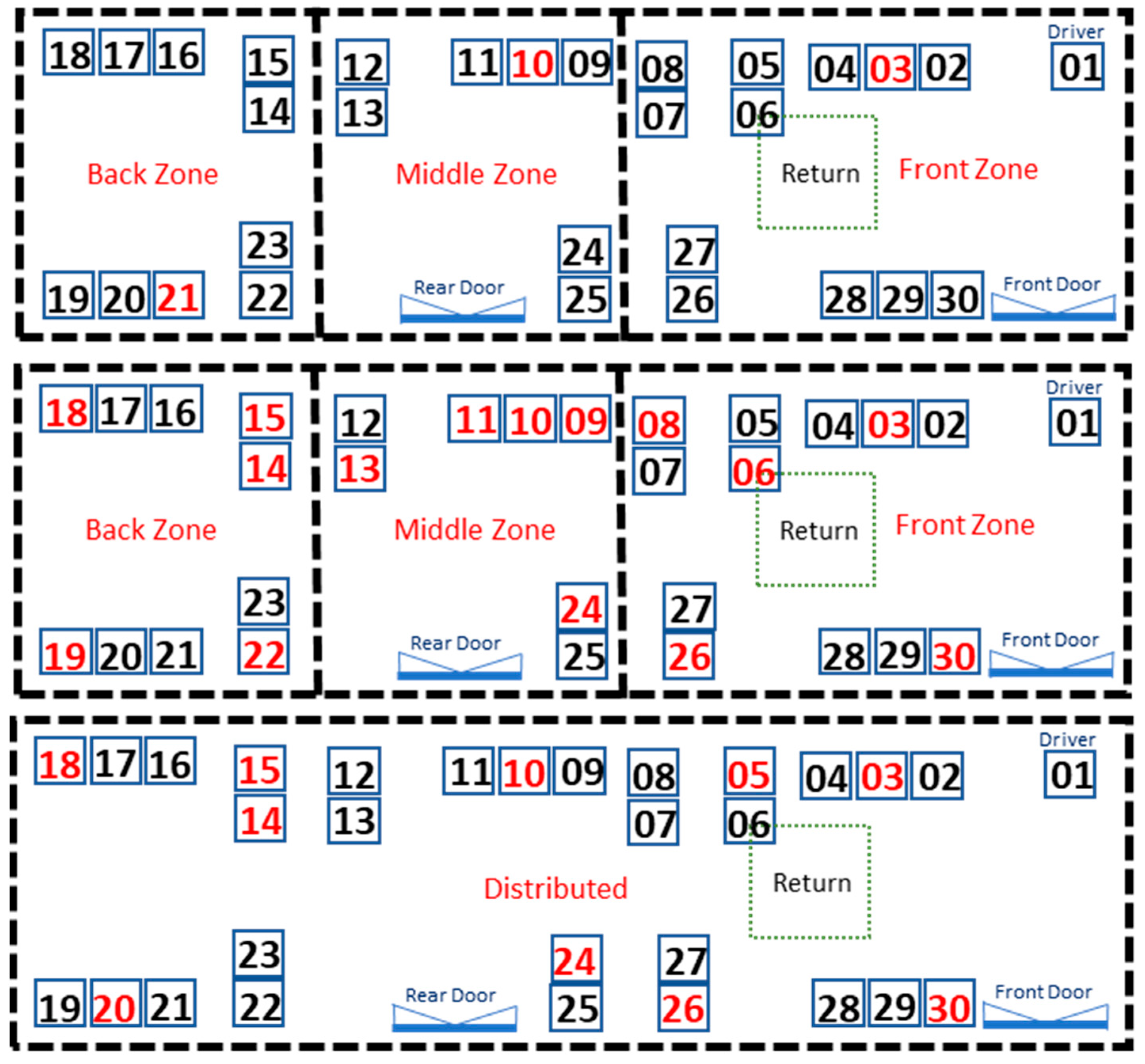
The following simulations all consider a bus at full seated capacity, with a seated passenger body model occupying each of the 30 seats in the vehicle. Among these occupants, the locations of infectious emitters are randomized to reflect the stochastic nature of passenger seating. We considered three scenarios involving one, five, and ten distinct infectious aerosol emitters. For cases of one and five emitters, we considered sub-cases where they are clustered in either the front, middle, or back sections of the bus. Ten emitters are too numerous to realistically be confined to a single region of the bus, so we distributed their location evenly throughout the vehicle for those respective scenarios. Figure 3 illustrates the emitter locations for these scenarios (red color). Particle injectors for infectious emitters are designed to emulate coughing. Emitted particles are assigned a diameter of 1 µm (size of viable airborne viral droplets as discussed previously).

Table 1 presents the four parameters that were independently varied in the present work so we could explore the extents of plausible infectious aerosol spatial distributions within in-service transit buses. The temperature of windows and air supply inlets were set to reflect either heating in the wintertime or cooling in the summertime. The recirculation air change rate on these buses is approximately 30 h⁻¹, but the actual recirculating fan speeds may vary due to thermal conditioning needs or system defects, so a range of high and low recirculation air change rates were considered. In total, 70 distinct scenarios were assembled and simulated using CFD software, STAR CCM+ 2020.3.1.

Through parametric analysis of various scenarios, this investigation delves into the often overlooked aspect of air quality within city buses. Recognizing that passengers’ well-being is intricately tied to the air they breathe during their daily commutes, this study seeks to uncover insights that can lead to positive changes in this environment. The investigation begins by examining the effects of temperature variations inside buses. By comparing different temperature settings, including heating and cooling scenarios, this study aims to decipher how these changes influence the distribution of particles in the air. This knowledge could ultimately contribute to more informed decisions about temperature control strategies that enhance passenger comfort. Next, the investigation explores the relationship between the supply airflow rate (in terms of ACH) and particle distribution. By manipulating the velocity of fresh air entering the bus, our work simulates various ACH values, shedding light on how different rates of air circulation impact the concentration of particles. This knowledge could guide improvements in ventilation systems that ensure a steady flow of clean air. Intriguingly, the investigation delves into the impact of the number and placement of particle-emitting sources. By altering the quantity of sources emitting particles and their locations within the bus, the study aims to uncover how these factors influence the overall particle concentration. This information could lead to strategies that minimize particle emissions and optimize source placement, contributing to a healthier indoor air environment. Ultimately, the investigation’s objective is to holistically understand the interplay between temperature, air exchange rates, particle-emitting sources, their locations, and the resulting air quality inside city buses. With these insights, public transportation authorities and vehicle designers can make informed decisions to create bus interiors that offer fresh, clean air to passengers. This aligns with the larger goal of providing commuters with a more pleasant, comfortable, and health-conscious journey, thus improving the quality of life for those who rely on buses for their daily travels.

A wide range of values were chosen for each parameter to ensure a thorough exploration. Air changes per hour (ACHs) were investigated across five values (0.1, 0.2, 0.3, 0.4, and 0.5 m/s), encompassing various ventilation rates, to comprehensively observe their effects on air and particle movement. Moreover, three distinct bus locations (front, middle, and back) with a normalized distance from the three emitter numbers (1, 5, and 10) were examined, representing realistic variations in seating arrangement and emitter density. These variations significantly impacted the dispersion of particles within the bus. Additionally, two different heating and cooling scenarios were integrated, offering valuable insights into their effects on particle movement and distribution.

For each scenario described in the Methods Section, 30 measurements (corresponding to each seat on the bus) of the simulated local concentration were collected. Each measurement was made by averaging the particle concentration values within a sample-sized sphere with a 20 cm radius centered around each passenger’s breathing zone. This sampling method is discussed in the following CFD modeling section. A total of 30 RC values were calculated from the 30 near-occupant measurements for each simulation, resulting in a dataset comprising 2100 RC data points used for the discussion and analysis.

2.3. Computational Fluid Dynamic Modeling

Geometry and Meshing

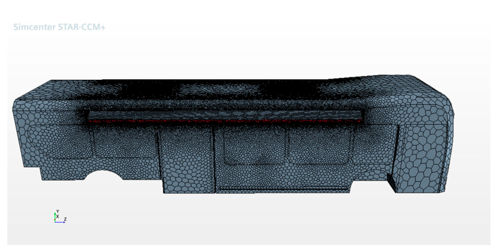
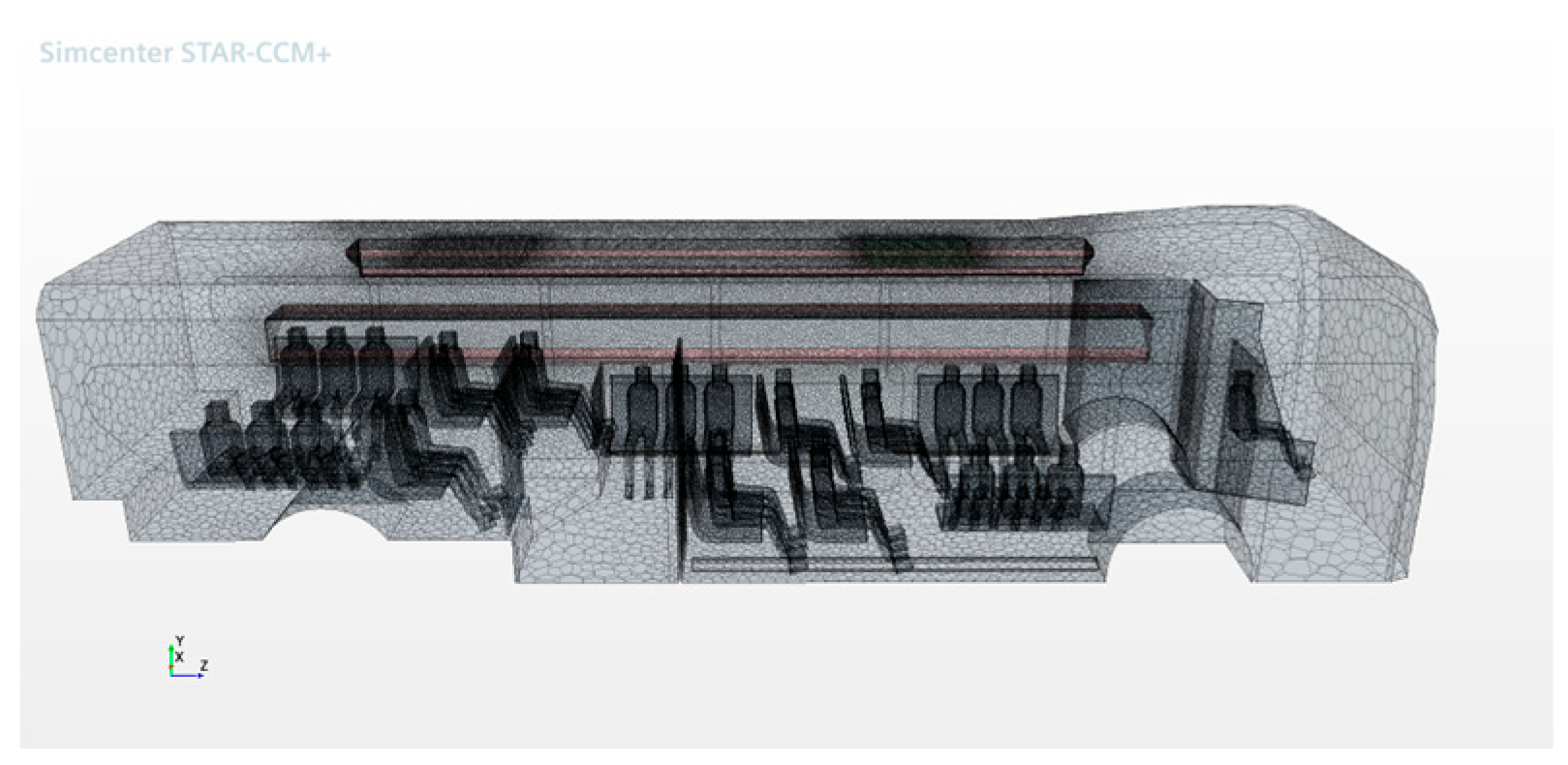
The commercial CFD package STAR CCM+ 2020.3.1 software by Siemens [39] was used for this work. The SEPTA provided a preliminary 3D model representing the bus geometry, which is imported to STAR CCM+ after surface repair to adhere to the requirement of CFD meshing. Three-dimensional models of seated passengers were then added to the bus interiors. An automatic mesher with polyhedral cells was used to generate the mesh (Figure 4 and Figure 5) with a higher resolution near the passengers’ mouths (particle inlets) and supply diffusers. The resulting mesh contained ~810 K cells which was verified for grid independence (50 k cells and 2 million cells) based on the similarity of air velocity (difference of <0.1 m/s) near occupants. Figure 4 and Figure 5 show the geometry and mesh used for the simulations.

2.4. General CFD Parameters and Convergence Criteria

Given the purpose of this work stated in Section 2.3, a steady-state solution was used by the CFD software. The Reynolds-averaged Navier–Stokes equation (RANS) model was used with the Realizable k-epsilon turbulence model as the region of interest is mostly the bulk airflow transport of the particles, and an enclosed bus can be considered similar to a typical indoor environment [40,41]. Due to the typical indoor thermal environment with small temperature and pressure variance, segregated solvers were used, incompressible gas was assumed, and Boussinesq approximation was employed for buoyancy and natural convection considerations. Finally, typical near-wall treatments for indoor environments were used [38]. The convergence of the simulations was considered based on the simulation residual of flow and particle mass. However, due to the use of the Lagrangian particle model with steady-state simulation, particle mass for a given monitored region is not steady-state but varied. Instead, the average of the last 50 iterations was used for convergence determination. This averaging approach is also used for the sampling process of particle concentration which will be discussed in a later section.

2.5. Particle Modeling

The Lagrangian particle model was selected due to its capacity for particle tracking as particle fate is of interest in this study. However, due to the intermittent release of the representative particle “packet” for particle tracking, temporal differences were introduced to a steady-state simulation that does not have time steps. This complication caused each iteration to have different results based on the specific location for a given particle “packet” and requires the averaging of any sampled particle concentration over many iterations. It was determined that the average of the last 50 iterations after convergence yields relatively constant results similar to steady-state results; hence, all results discussed in the following sections are averages of the last 50 iterations of a given simulation.

2.6. Sampling Particles in CFD Simulation

Due to the use of the Lagrangian particle model and the particle “packets” present in variable locations for a given iteration, it is important to sample the particle concentration over a specific space instead of a single point. In this study, spherical sample zones surrounding the heads of each passenger were created for this spatial averaging approach to capture relevant particle “packets”, allowing for a more accurate representation of the particle concentration which can interact with rider inhalation. Each sample zone encompasses a three-dimensional space centered around the nose and mouth of an individual. This approach acknowledges the inherent complexities of particle dispersion within the bus cabin. Passengers are assumed to be seated and stationary in their designated location for this analysis domain, approximating typical behavior on a moving bus; so, the sample zone used can be said to adequately represent the inhalable particles for each passenger. This method is more precise than the typical breathing plane approach [42] as particles outside of the seated area are excluded. Figure 6 demonstrates the spherical sampling zone used around each passenger.

Infectious particle concentrations at different locations were obtained by averaging the concentration across the respective volume. The integral concentration of particles within a specific volume in the breathing zone is determined using Equation (1):

$$Q=\int \int \int VC(x,y,z)dV$$

(1)

Here, the triple integral covers the volume V, and C (x, y, z) is the concentration distribution function in three dimensions. This equation enables us to quantify the cumulative particle concentration within a specific volume of the bus.

2.7. Boundary Conditions and Settings

A particle’s size rather than its chemical composition (ignoring the impact of semi-volatile constituents) is the dominant factor for airborne particle transport. Also, we are interested in the overall particle distribution instead of a specific species; therefore, NaCl particles were selected due to their prevalent use in particle experimental studies [43,44]. Various emission parameters, such as velocity and flow rate, were controlled in accordance with recent research [45].

Table 2. Boundary conditions.

Boundary Name	Boundary Conditions	Physics Values
BUS- New Flyer Xcelsior 40’ [1]	Region	Length: 14 m Height: 3 m Width: 2.6 m Volume: 109.2 m3
Outlet	Outlet; Mass Flux Specification	Split Ratios: 0.0
Return Air Outlet	Outlet; Mass Flux Specification	Split Ratios: 1.0
Inlet Air Supply Opening	Velocity Inlet	Velocity: 0.1, 0.2, 0.3, 0.4, 0.5 m/s Equivalent ACH: 5.74, 11.47, 17.20, 22.93, 28.66 h−1 Temperature: 80 °F, 50 °F, 90 °F Turbulence Intensity: 0.01 Turbulent Viscosity Ratio: 10.0
Windows; Doors; Rear Window; Windshield	Wall; Shear Stress Specification: No-Slip Wall; Standard Wall Function	E: 9.0 Kappa: 0.42 Temperature: 80 °F, 50 °F, 90 °F
Bus: Front, Back, Left, Right, Top, Floor, Dividers, Seats, AC Surfaces Passengers: Body, Head	Wall; Shear Stress Specification: No-Slip Wall; Blended Wall Function	E: 9.0 Kappa: 0.42 Temperature: 80 °F
Injectors	Injector; Mass Flow Rate	Emitter Mass Flow Rate: 3.33 × 10−10 kg/s Passenger Mass Flow Rate: 0.0 kg/s Particle Diameter 1.0 um Particle Temperature 80 °F Velocity: 0.1 m/s Parcel Streams: 12.0 Direction: [−1.0, 0.0, 0.0]
Emitters’ Mouths	Mass Flow Inlet; Turbulence Specification Method: Intensity + Viscosity Ratio	Emitter Mass Flow Rate: 2.04 × 10−4 kg/s Temperature: 80 °F Turbulence Intensity: 0.01 Turbulent Viscosity Ratio: 10.0
Volume Fraction Sampling Domain	Field Function, Spherical Domain	Radius: 20 cm Center: Emitter’s Mouth

presents the boundary conditions that were applied to the CFD model domain to constrain airflow and reflect realistic conditions.

3. Results

3.1. Explanation of Results from Simulations

The postprocessing analysis has been conducted to calculate the relative concentration (RC) for each seated passenger and the spatial RC distribution. Indeed, this is considered throughout the bus for each sampling sphere related to the seated riders. Visualization of this sampling zone is illustrated in Figure 7.

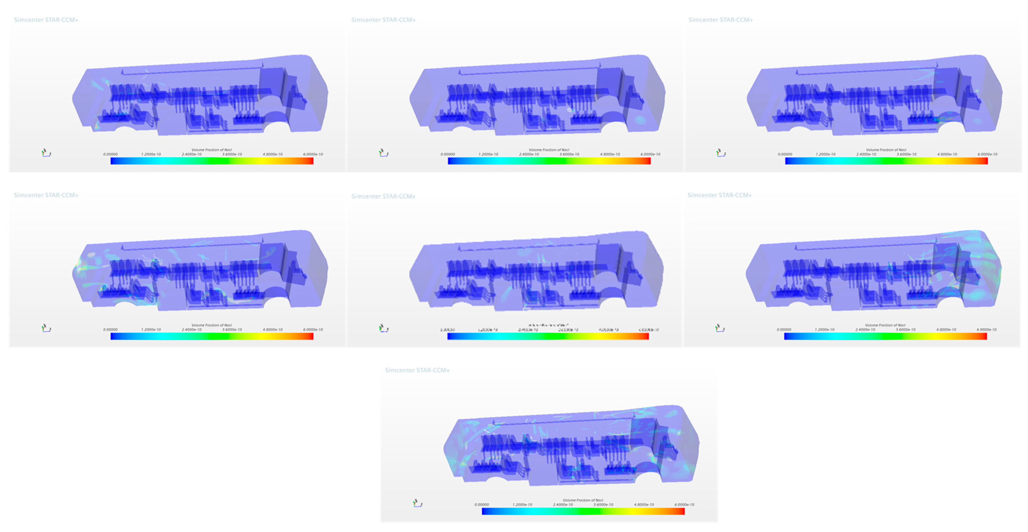
Furthermore, the simulation can produce the spatial concentration for the entire bus which can be used to visually see the concentration zone inside the bus; an example of these results is shown in Figure 8 where different emission scenarios are compared.

3.2. Parametric Analysis Based on RC

The objective of this analysis is to understand the relationship between the relative concentration (RC) of particles and various environmental and operational parameters in a bus. RC serves as the main independent variable, and its correlations with other parameters such as air changes per hour (ACHs), the number of emitters, the distance from the seat to the return area, emitter location, and thermal conditions have been examined. The data used for this analysis were collected from a postprocessing CFD result of the simulations. The dataset includes both numerical and categorical variables that influence RC. The categorical variables were encoded using label encoding to allow for a unified correlation analysis alongside numerical variables.

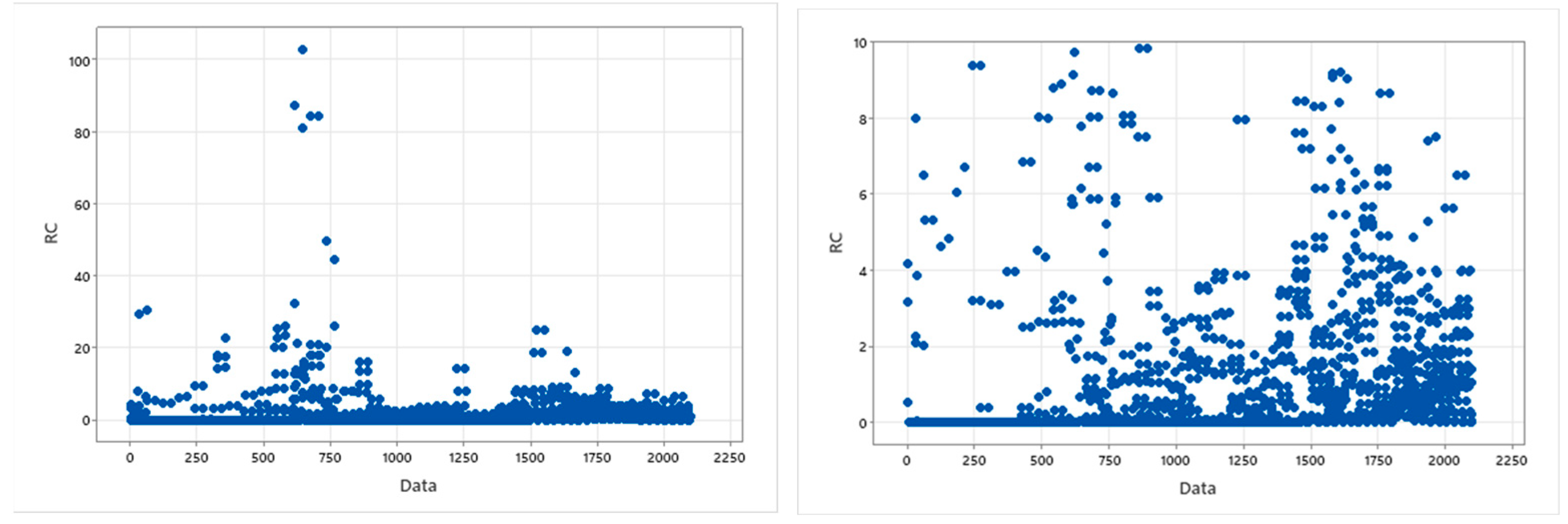
The scatter plot in Figure 9 displays the relative concentration (RC) of aerosols across different data points, where each point represents a sample size zone for each seat. This means that the ‘Data’ variable indexes various seat locations within the bus environment, and RC represents the relative concentration measured at those specific locations for different scenarios. The observation of RC distribution shows that the majority of RC values lie between 0 and 10, indicating that low RCs are common across most seat locations in the dataset. There are some notable outliers where RC values exceed 10, with a few points reaching up to 100. These outliers suggest that certain seat locations have significantly higher RC values.

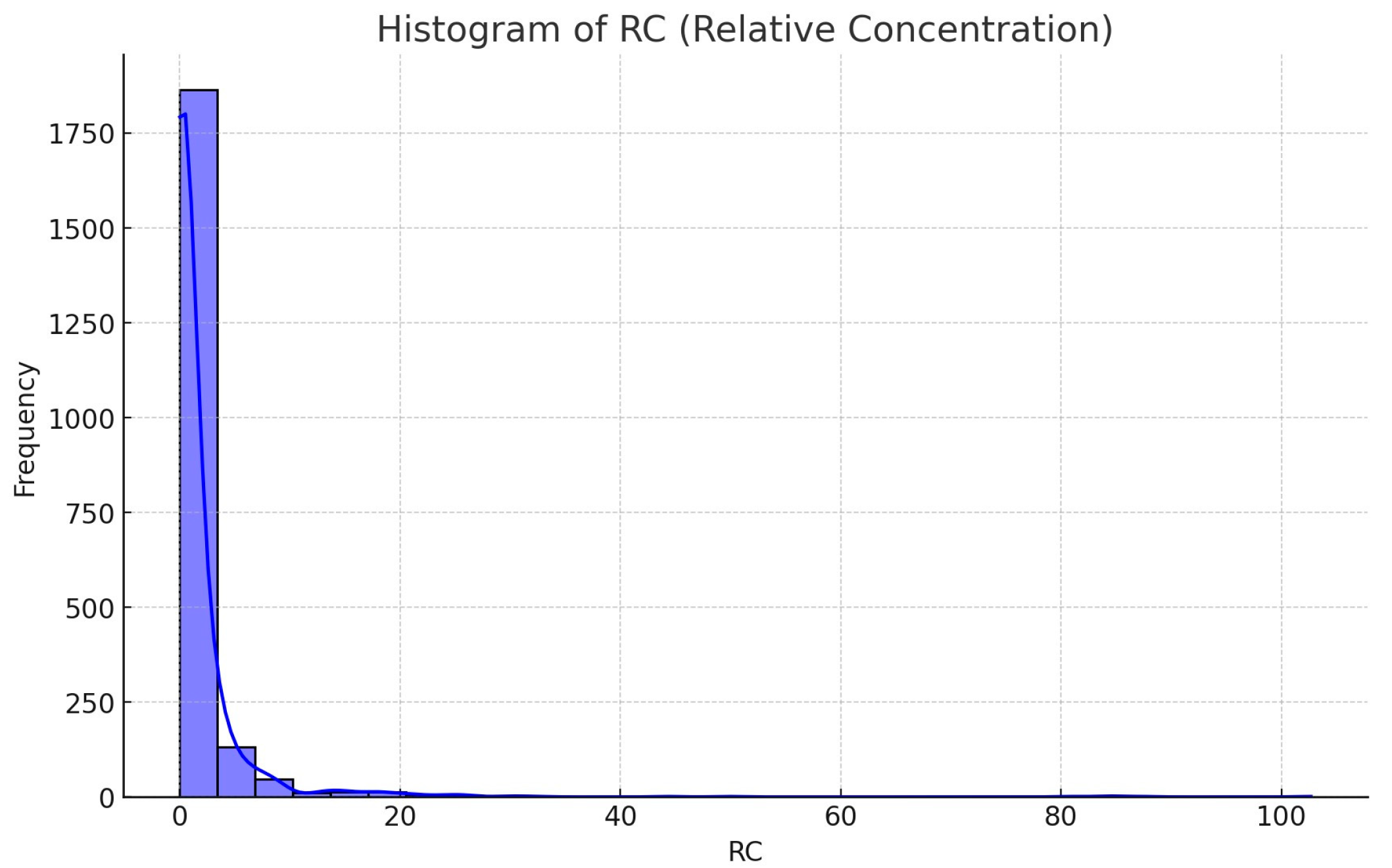
Furthermore, the histogram produced and displayed in Figure 10 represents the distribution of relative concentration (RC) values across different seat locations or sample zones within a bus transportation environment.

This visualization provides insights into how frequently different levels of RC occur throughout the dataset. Here are the observations of the histogram:

• Skewed Distribution: The histogram shows a highly skewed distribution, with the majority of RC values concentrated near the lower end of the scale. Most RC values are clustered between 0 and 5, indicating that low aerosol concentrations are very common in the dataset.
• High Frequency of Low RC Values: The frequency of RC values at or near 0 is exceptionally high, with over 1750 instances recorded. This suggests that a significant portion of seat locations or zones experience very low aerosol concentrations. The rapid decline in frequency as RC values increase indicates that higher RC values are much less common.
• Long Tail: The histogram features a long tail extending to the right, with RC values ranging up to 100. Although these high RC values are rare, they represent outlier conditions where aerosol concentration is significantly elevated. The presence of these outliers highlights specific instances or seat locations with unusually high aerosol concentrations, which could be influenced by factors such as emitter proximity, ventilation inefficiencies, or localized environmental conditions.

3.3. Descriptive Analysis of Dataset

Table 3. Descriptive analysis of numerical factors impacting RC.

Column	Data	ACH (h−1)	Number of Emitters	Dis. from SEAT to the Center of Return	RC
count	2100	2100	2100	2100	2100
mean	1050.5	17.1960574	4	3.075384778	1.625865
std	606.3621	8.105767887	3.07132925	1.145031063	5.541296
min	1	5.735497	1	1.781628469	0
25%	525.75	11.46578	1	2.15264953	0
50%	1050.5	17.19606	5	2.604995558	0.030781
75%	1575.25	22.92634	5	3.891747679	1.318705
max	2100	28.65661	10	5.297065225	102.6799

provides a detailed statistical summary of the key variables in the dataset, which includes data points related to the relative concentration (RC) and various numerical factors influencing it, such as air changes per hour (ACHs), the number of emitters, and the distance from the seat to the return area.

The key insights are as follows:

• ACH (h⁻¹): The distribution is slightly skewed, with most values clustered around the mean of 17.2.
• Number of Emitters: The distribution is right-skewed, with most values at the lower end and fewer high values.
• Dis. from Seat to Return Area: The distribution is slightly right-skewed, with most values around the mean of 3.08 m.
• RC: The distribution is highly skewed, with many instances of low values and a few extremely high values, indicating significant variability and potential outliers.

3.4. Statistical Analysis

To quantify the relationships between RC and other parameters, we computed the Pearson and Spearman correlation coefficients. The Pearson correlation measures the linear relationship between variables, while the Spearman correlation assesses monotonic relationships. Both coefficients provide insight into how changes in the independent variables might affect RC.

Table 4. Pairwise table for Pearson and Spearman correlations between RC and other features.

Feature	Pearson Correlation	Pearson p-Value	Spearman Correlation	Spearman p-Value
ACH (h−1)	−0.068	0.002	−0.105	<0.001
Number of Emitters	−0.049	0.034	−0.045	0.043
Dis. from Seat to Return Area	0.127	<0.001	0.164	<0.001
Emitter Location	−0.164	<0.001	−0.198	<0.001
Thermal Condition	−0.007	0.787	0.002	0.923

represents the pairwise table for the Pearson and Spearman correlations between RC and other features. To perform the parametric analysis, we can explore the relationships between RC (relative concentration) and other factors using correlation analysis and visualizations.

3.5. Correlation Analysis

The correlation matrix has been summarized in

Table 5. Correlation matrix for variables.

Feature	RC
ACH (h−1)	−0.06795
Number of Emitters	−0.0489
Dis. from Seat to Return Area	0.127272
Emitter Location	−0.16392
Thermal Condition	−0.00683

to see how each factor correlates with RC.

3.6. Visualizations

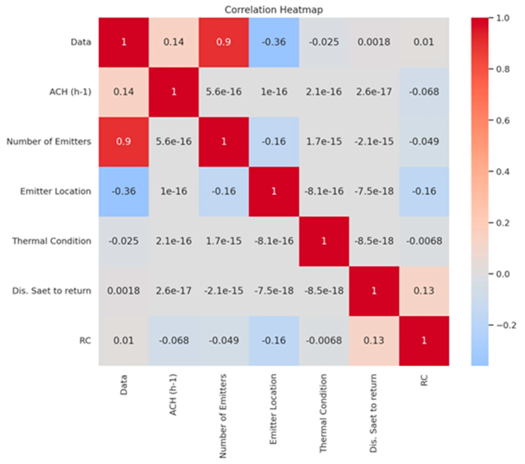
The heatmap plots in Figure 11 have been created to visualize the relationships between RC and other factors.

The correlation heatmap indicates that RC has weak correlations with most variables, suggesting that it is largely independent of factors like ACHs, emitter location, and thermal conditions. A small positive correlation (0.13) with “Distance from Seat to Return” suggests that RC may have a minor relationship with airflow patterns based on seating proximity to return vents.

3.7. RC and Different Air Change Per Hour Scenarios (ACH (h⁻¹))

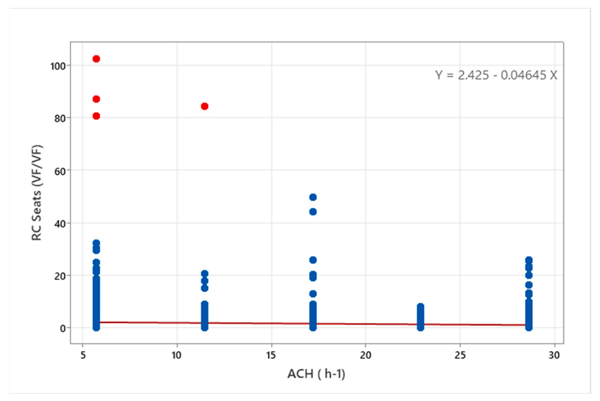
This section explores the relationship between RC and air exchange. Indoor pollutant fundamentals necessitate that, in most cases, higher air exchange leads to lower concentrations. This phenomenon is quantified for infectious aerosols in the bus domain in Figure 12. However, it is noteworthy that at the maximum ACH, there is an uptick in the RC, signifying a higher concentration of particles compared to the return, even though the overall particle concentration is reduced due to enhanced ventilation and air circulation. Worse scenarios occur in the back zone of the bus where the particles are lingering due to low flow rates and inadequate ventilation. The poor ventilation in that zone causes the particles to remain there for a prolonged period of time These finding underscore the importance of efficient air exchange in mitigating particle concentration and promoting better air quality in the breathing and dead zone, and highlight the nuanced relationship between ACH and relative particle concentration.

The ACH and RC correlation can be determined by using the Pearson and Spearman correlation coefficients from Table 4 and Figure 13. A positive Pearson correlation suggests that as ACH increases, RC also tends to increase, and vice versa. Conversely, a negative correlation signifies an inverse relationship. The Spearman correlation coefficient, on the other hand, assesses the monotonic relationship between ACH and RC. Unlike the Pearson correlation, Spearman does not assume a linear association. It detects whether changes in ACH and RC tend to move in the same direction, irrespective of the form of the relationship.

Based on Table 4 and the analysis of RC Seats (VF/VF) and ACH (h⁻¹), the Pearson correlation coefficient is −0.068, indicating a weak negative relationship, and it is statistically significant, with a p-value of 0.002. However, the Spearman correlation suggests a weaker and non-significant negative correlation, with a coefficient of −0.040 and a p-value of 0.878. It can be determined that there is no significant relationship between air changes per hour (ACHs) and relative concentration (RC). In other words, changes in ACH values do not seem to have a strong impact on the distribution of particles, as indicated by the low correlation values. These findings suggest that, within the range of ACH values studied, altering the rate of air exchange does not substantially affect how particles are dispersed or concentrated within the bus environment. While ACH is an important factor for maintaining air quality, it appears that other variables, such as emitter positions and numbers, have a more pronounced influence on particle distribution. This insight is valuable in refining our understanding of the complex dynamics governing air quality in buses. While ACH remains a crucial parameter for overall ventilation and comfort, our research indicates that its direct influence on particle distribution, as measured by RC, is relatively limited. This understanding can guide future efforts to optimize air quality management strategies within bus interiors.

3.8. RC and Different Numbers of Emitter/s

Similarly, the Pearson and Spearman correlation coefficients were applied to examine the potential relationship between the number of emitters and relative concentration (RC), as shown in Figure 14. This statistical approach aimed to quantify any possible connection between these two variables.

The analysis of the correlation between RC Seats (VF/VF) and the number of emitters revealed different results based on the Pearson and Spearman correlation coefficients. Based on Table 4, the Pearson correlation coefficient of −0.049 suggests a weak negative relationship, indicating that as the number of emitters increases, RC tends to decrease slightly. Importantly, this negative correlation is statistically significant, with a p-value of 0.025, signifying that the observed relationship is unlikely to have occurred by random chance. Conversely, the Spearman correlation coefficient of 0.407 points to a strong positive correlation, implying that as the number of emitters increases, RC also tends to increase. This positive relationship is highly statistically significant, with a p-value of less than 0.001, underscoring its reliability. These contrasting results highlight the importance of considering different correlation methods and the potential impact on the interpretation of the relationship between these variables. Further investigation such as linear regression is performed to gain a deeper understanding of the factors influencing this relationship. The regression equation, RC Seats (VF/VF) = 1.979 − 0.08822 × Number of Emitters, quantifies the relationship and implies that for each additional emitter, RC Seats are expected to decrease. This result might not align with the goal of reducing particle concentration, as it suggests that more emitters lead to a decrease in RC.

It can be concluded that there is no significant relationship between relative concentration (RC) and different numbers of emitters. In simple terms, the data suggest that changes in the number of emitters do not appear to strongly affect the distribution of particles, as indicated by the low correlation values. This finding implies that the quantity of particle-emitting sources, whether high or low, does not seem to have a substantial impact on how particles are distributed and concentrated within the bus environment. Other factors, such as emitter positions, might have a more pronounced influence on particle distribution.

3.9. Distance Between Each Seat and the Return

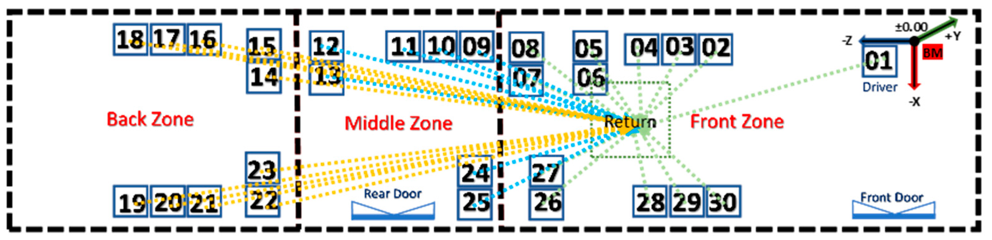
In the other step, the distance between each seat and the return was calculated. This involved measuring the physical distance between each seat and the center point of the return area. This step helped us understand how particles from various seats interacted with the return system. To achieve this, a location framework was employed, referencing the distance between emitters’ mouths and the center of the return area within the bus (Figure 15). Furthermore, a benchmark point was established at the right corner of the bus, and all measurements were calculated based on the x, y, and z dimension values at the BM.

To find the distance between the points with coordinates (x₁, y₁, z₁) and (x₂, y₂, z₂) given in a 3D plane, a 3D distance formula can be applied, given as follows:

$$d=\sqrt{[{(x_2-x_1)}^2+{(y_2-y_1)}^2+{(z_2-z_1)}^2]}$$

The Bench Mark (BM) coordinate is (x₂ = 0, y₂ = 0, z₂ = 0).

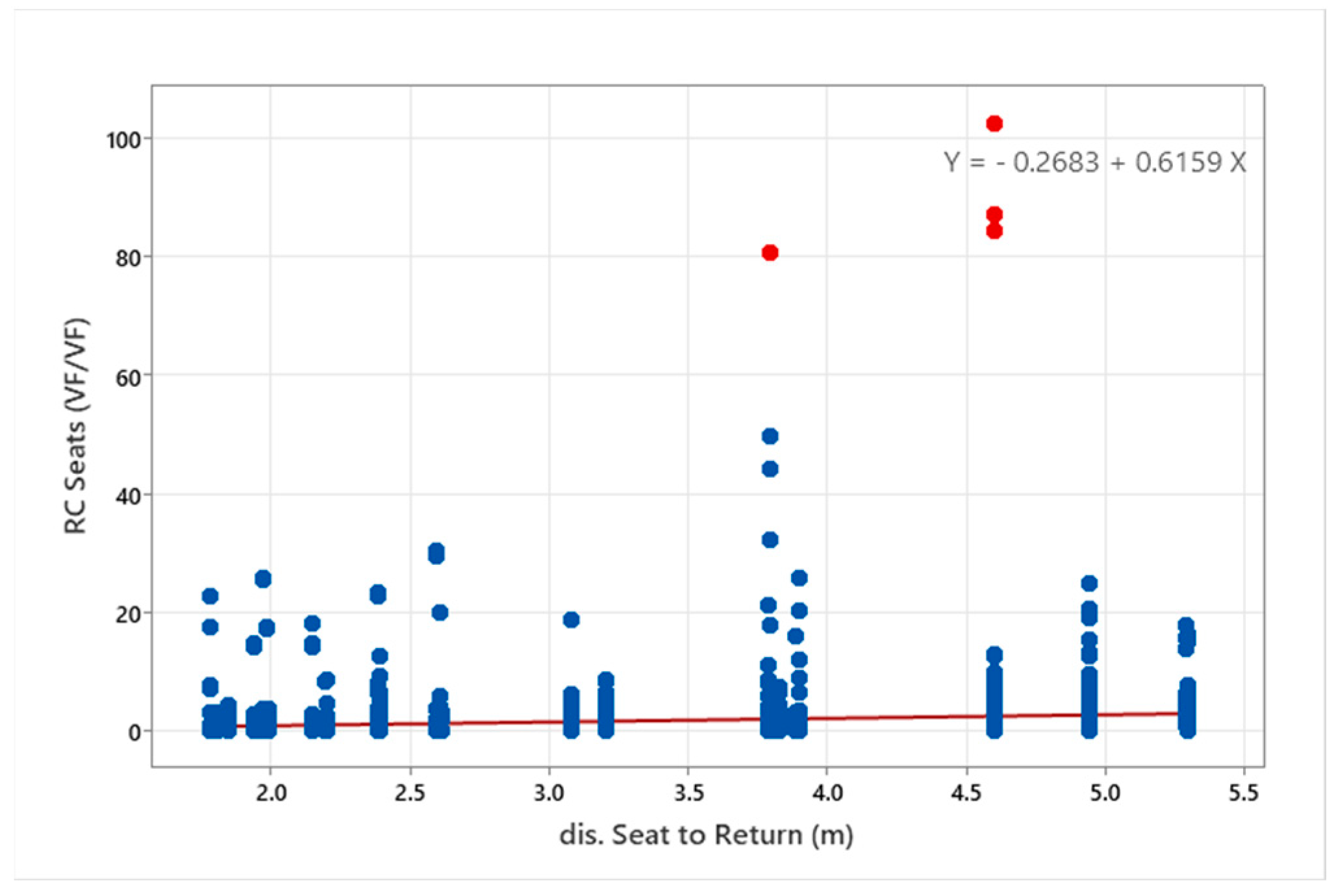
Additionally, the analysis of Figure 16 suggests that the distance from the return area has a significant impact on relative concentration (RC). As one moves further from the return area, there is a noticeable increase in RC, indicating a correlation between seating positions based on return and particle relative concentrations. Furthermore, the data reveal that the back and middle positions with a single emitter have a more substantial influence on RC compared to other configurations. This finding underscores the importance of considering rider placement, especially in the back and middle areas of the bus, as they are key parameters identified in the observed variations that affect particle concentration.

The correlation analysis between relative concentration (RC) and the distance between seats and the return area revealed valuable insights. Based on Table 4, the Pearson correlation coefficient of 0.127 indicates a weak positive linear relationship between these two variables, implying that as the distance between seats and the return area increases, there is a slight tendency for RC to also increase. This correlation is statistically significant (p < 0.001), suggesting the potential influence of seating configurations on particle concentration. Conversely, the Spearman correlation coefficient of −0.035 suggests a weak negative relationship between RC and seat-to-return distance, although this correlation is not statistically significant (p = 0.105). The Spearman correlation, which is based on rank order rather than precise values, implies that the relationship is not well described by a linear trend. This visualization can be seen in Figure 17.

The linear regression equation “RC Seats (VF/VF) = −0.268 + 0.616 dis. Seat to Return (m)” provides a predictive model for RC based on seat-to-return distance. Each unit increase in distance corresponds to a 0.616 unit increase in RC, as indicated by the positive coefficient. This suggests that, while the correlation is weak, there is some predictive capacity for RC based on seat positioning. In summary, the analysis highlights a weak but statistically significant correlation between seat-to-return distance and RC. However, the relationship is not purely linear, suggesting the involvement of other complex factors that merit further investigation to better understand particle dispersion in enclosed transit spaces.

3.10. RC and Different Emitter Locations

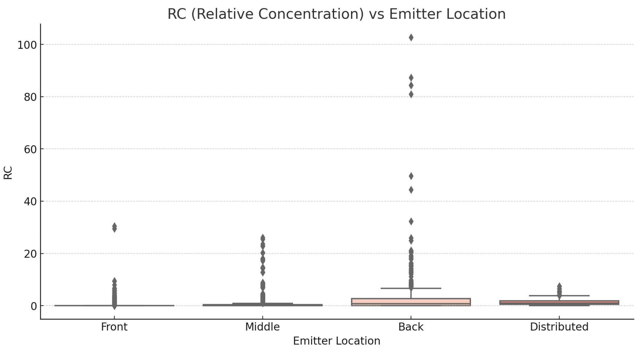
Since emitter location comprises categorical data, the box plot visualization in Figure 18 highlights the impact of emitter location on RC values. It provides a clear comparison of how different locations influence the distribution of relative concentration.

The image shows a box plot of RC (relative concentration) values against different emitter locations (front, middle, back, and distributed). Here are some key observations:

• Front: The RC values are generally low with some outliers, indicating occasional higher concentrations. The median value is close to zero, with a narrow interquartile range (IQR).
• Middle: Similar to the front location, RC values are low with several outliers.

The median value is close to zero, and the IQR is slightly wider than for the front location.

• Back: The back location shows higher RC values compared to other locations, with several significant outliers. The median value is higher, and the IQR is much wider, indicating greater variability in RC values.
• Distributed: RC values are consistently low, with few outliers. The median value is close to zero, with a narrow IQR, similar to the front location.

Also, the correlation coefficient matrix has been calculated to find the exact value of correlation between location variables and RC, along with creating a visualization graph (

Table 6. Correlation coefficient for categorical location variable.

Feature	Correlation with RC
Emitter Location_Back	0.191811
Emitter Location_Distributed	−0.01498
Emitter Location_Front	−0.12476
Emitter Location_Middle	−0.05545

and Figure 19).

Figure 19 presents the bar plot related to the correlation matrix for visualization.

This bar plot visualizes the correlation coefficients between RC (relative concentration) and different emitter locations:

• Emitter location at the back has a positive correlation with RC, indicating higher RC values when the emitter is located at the back.
• A distributed emitter location has a near-zero correlation with RC, suggesting minimal impact on RC values.
• Emitter location at the front has a negative correlation with RC, indicating lower RC values when the emitter is located at the front.
• Emitter location at the middle also has a negative correlation with RC, suggesting lower RC values when the emitter is in the middle.

The gray dashed line at zero represents the baseline for no correlation, highlighting the differences in correlation for each emitter location. This visualization helps to easily compare the impact of different emitter locations on RC values.

In summary, the back location tends to have higher and more variable RC values, indicating a potential area of concern for higher relative concentrations. The front and middle locations show lower RC values but still have occasional higher concentrations.

The distributed location has the most consistent and lowest RC values, suggesting more uniform dispersion. This graph provides a clear comparison of how different locations influence the distribution of relative concentration.

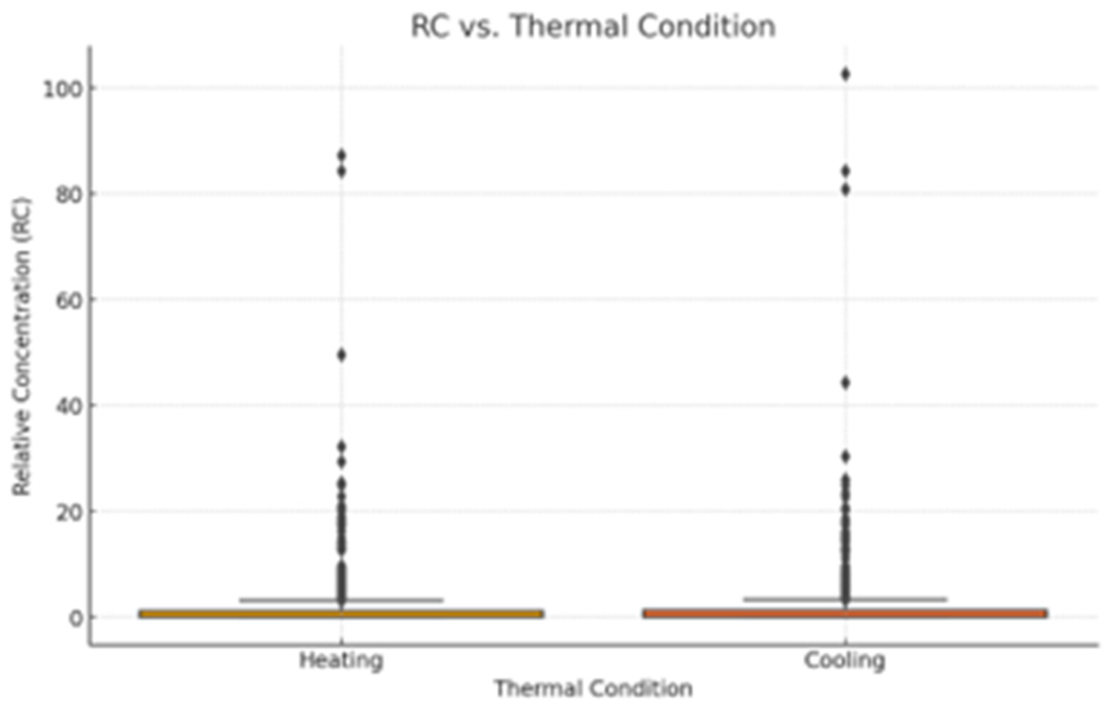
3.11. RC and Heating and Cooling Scenarios

The heating and cooling scenarios have been simulated, and the categorical results in Figure 20 and

Table 7. Correlation matrix for thermal conditions.

Thermal Condition	Correlation with RC
Thermal Condition_Cooling	0.006829
Thermal Condition_Heating	−0.00683

show the differences in relative concentration for each seat between these two scenarios. The data indicate that these factors have a negligible effect on the dispersion and distribution of particles, particularly when considering RC. This study identifies two critical observations: First, the high total air exchange rate utilized results in forced convection overwhelmingly governing the bulk air transport between seats within the bus, thereby rendering the influence of thermal natural convection negligible. Second, while localized airflow—such as that near heat sources, windows, or in the immediate vicinity of passengers—is affected by thermal conditions, its influence on the overarching airflow distribution throughout the bus is minimal and does not significantly impact the study’s primary focus on whole-bus ventilation patterns.

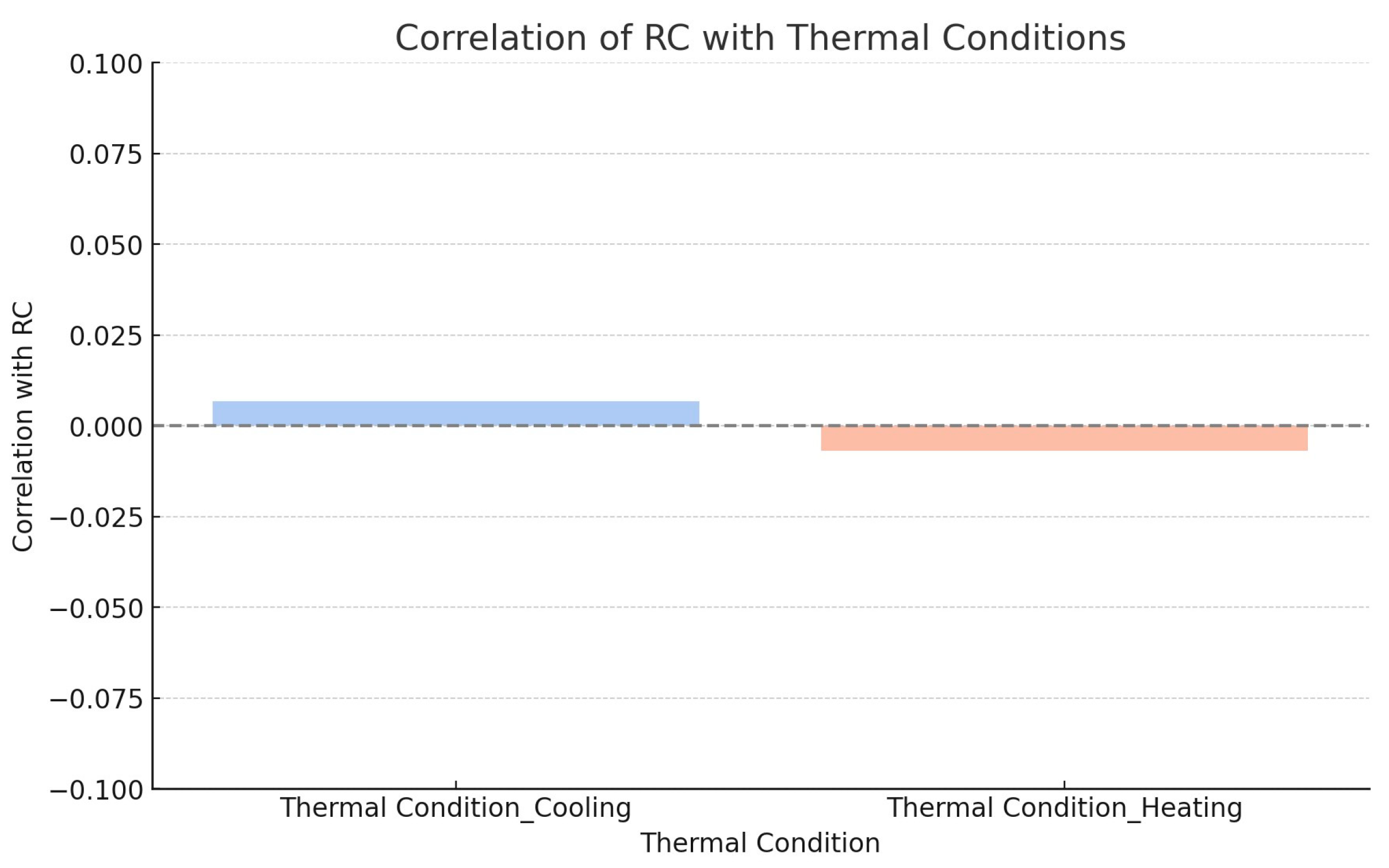
Figure 21 shows the bar plot related to the correlation matrix for visualization.

Figure 21 illustrates the correlation between RC and thermal conditions (cooling and heating). Here is the summary of the findings:

• Thermal Condition_Cooling: Correlation with RC: 0.006829

Interpretation: There is a very weak positive correlation between cooling thermal conditions and RC. This suggests that cooling conditions do not significantly affect RC values.

• Thermal Condition_Heating: Correlation with RC: −0.00683

Interpretation: There is a very weak negative correlation between heating thermal conditions and RC. This suggests that heating conditions do not significantly affect RC values.

In summary, the correlation coefficients for both thermal conditions (cooling and heating) are very close to zero, indicating that neither condition has a significant impact on RC values. The minimal differences in correlation suggest that the relative concentration is largely unaffected by whether the environment is being heated or cooled.

4. Discussion

In this study, a parametric analysis was conducted to understand the factors impacting the spatial distribution of particles within a bus environment. Using computational fluid dynamics (CFD) simulations, it evaluated the effects of various parameters, including air changes per hour (ACHs), the number and location of particle emitters, and thermal conditions on the relative concentration (RC) of particles. The findings from this investigation provide valuable insights into the dynamics of particle distribution in public transportation systems and offer practical implications for improving air quality and mitigating the spread of airborne pathogens.

Our results indicate that increasing the air change rate (ACH) leads to a general decrease in the overall particle concentration within the bus cabin. Specifically, increasing the ACH rate from 5.74 h⁻¹ to 28.66 h⁻¹ resulted in a reduction in the absolute particle concentrations of approximately 45%. However, the impact on RC, which measures the deviation from a well-mixed concentration, is less pronounced. For instance, while the absolute particle concentration decreased, localized areas of higher concentration were still observed. At an ACH rate of 28.66 h⁻¹, the maximum RC value observed was 1.57, indicating areas where particle concentration was 57% higher than the well-mixed average. This suggests that while increasing ventilation rates can reduce overall particle levels, it may not completely eliminate pockets of higher concentrations, especially in areas with poor mixing. This highlights the importance of optimizing ventilation systems not just for overall air exchange but also for ensuring uniform air distribution throughout the cabin.

The number and spatial distribution of particle emitters significantly influence the particle concentration profiles within the bus environment. Scenarios with multiple emitters distributed throughout the cabin showed a more even distribution of particles, with RC values averaging around 0.95, indicating near-uniform mixing. In contrast, scenarios with clustered emitters resulted in localized high concentrations, with RC values exceeding 2.0 in certain areas. This finding underscores the importance of considering passenger seating arrangements and emitter locations when designing ventilation strategies. For instance, ensuring that emitters (such as passengers exhaling particles) are evenly distributed can help in achieving a more uniform particle distribution and reducing high-concentration zones.

Thermal conditions, represented by heating and cooling scenarios, were found to have a relatively minor effect on the RC of particles. The average RC values under different thermal conditions were 1.664 for cooling and 1.588 for heating, with a percent difference of only about 4.68%. This small difference, despite being statistically significant (p-value < 0.05), suggests that temperature variations within the typical range experienced in public transportation do not substantially impact particle dispersion. This implies that other factors, such as air exchange rates and emitter distribution, play a more critical role in determining particle concentration profiles.

The use of RC as a metric allowed for a clearer comparison of particle distribution across different scenarios. An RC value of 1 indicates a well-mixed state, while values greater than 1 indicate areas of higher concentration and values less than 1 indicate areas of lower concentration. This metric proved effective in highlighting the non-uniformity of particle distribution and identifying areas within the cabin that are more prone to higher concentrations of particles. For example, in a scenario with five emitters clustered in the front section of the cabin, the RC value in that area reached up to 2.5, indicating a concentration 2.5 times higher than the well-mixed average. The findings reveal that even with increased ventilation, certain areas could still experience higher RC values, indicating the need for targeted interventions in those specific zones.

The insights gained from this study have several practical implications for the design and operation of ventilation systems in public transportation. Firstly, optimizing air exchange rates is crucial, but it should be coupled with strategies to enhance air mixing and avoid localized high concentrations. Secondly, the placement of passengers and emitters should be considered in ventilation design to ensure a more uniform distribution of particles. Lastly, while thermal conditions may not significantly impact particle dispersion, maintaining a comfortable thermal environment is still essential for passenger comfort and overall system efficiency.

Future research should explore the integration of real-time monitoring systems to dynamically adjust ventilation based on passenger load and distribution. Additionally, studies could investigate the effects of different particle sizes and types, as well as the interactions between particles and surfaces within the cabin. The development of more sophisticated models that incorporate human behavior and movement patterns could also provide deeper insights into particle dynamics in public transportation settings.