Article

Application of Long Short-Term Memory and XGBoost Model for Carbon Emission Reduction: Sustainable Travel Route Planning

Department of Computer Engineering, Manisa Celal Bayar University, 45140 Manisa, Türkiye
*
Author to whom correspondence should be addressed.
Sustainability 2025, 17(23), 10802; https://doi.org/10.3390/su172310802
Submission received: 23 October 2025 / Revised: 21 November 2025 / Accepted: 25 November 2025 / Published: 2 December 2025
(This article belongs to the Special Issue Design of Sustainable Supply Chains and Industrial Processes)

Abstract

Travel planning is a process that allows users to obtain maximum benefit from their time, cost and energy. When planning a route from one place to another, it is an important option to present alternative travel areas on the route. This study proposes a travel route planning (TRP) architecture using a Long Short-Term Memory (LSTM) and Extreme Gradient Boosting (XGBoost) model to improve both travel efficiency and environmental sustainability in route selection. This model incorporates carbon emissions directly into the route planning process by unifying user preferences, location recommendations, route optimization, and multimodal vehicle selection within a comprehensive framework. By merging environmental sustainability with user-focused travel planning, it generates personalized, practical, and low-carbon travel routes. The carbon emissions observed with TRP’s artificial intelligence (AI) recommendation route are presented comparatively with those of the user-determined route. XGBoost, Random Forest (RF), Categorical Boosting (CatBoost), Light Gradient Boosting Machine (LightGBM), (Extra Trees Regressor) ETR, and Multi-Layer Perception (MLP) models are applied to the TRP model. LSTM is compared with Recurrent Neural Networks (RNNs) and Gated Recurrent Unit (GRU) models. Root Mean Square Error (RMSE), Mean Absolute Error (MAE), Mean Squared Error (MSE), and Normalized Root Mean Square Error (NRMSE) error measurements of these models are carried out, and the best result is obtained using XGBoost and LSTM. TRP enhances environmental responsibility awareness within travel planning by integrating sustainability-oriented parameters into the decision-making process. Unlike conventional reservation systems, this model encourages individuals and organizations to prioritize eco-friendly options by considering not only financial factors but also environmental and socio-cultural impacts. By promoting responsible travel behaviors and supporting the adoption of sustainable tourism practices, the proposed approach contributes significantly to the broader dissemination of environmentally conscious travel choices.

1. Introduction

Traveling is a great opportunity to discover new cultures, taste different flavors and have unique experiences. However, to make this experience perfect, it is necessary to make important decisions and take care of many details. Getting lost in unknown places, choosing the right activities and deciding on the most suitable route can be time-consuming and challenging. Additionally, choosing the wrong routes and traveling unnecessary distance may lead to an increase in carbon footprint and environmental impacts. Many sectors need models that provide optimum solutions for cost, time and energy savings [1,2]. In addition to providing the demands of users, it is important to present eco-friendly models. Economic and technological resources guide users’ travel planning. Especially in the tourism sector, some difficulties may arise when tourists individually plan their visiting unfamiliar places [3,4].
In recent years, the increasing visual and textual touristic trip data provided by users, along with advancements in data mining and machine learning techniques, has led to the growing use of travel recommendation systems. These systems aim to offer personalized travel experiences to travelers based on their individual preferences, past behaviors, and environmental factors [5]. However, while the tourism sector makes significant contributions to the global economy, its environmental impact has also been gaining increasing attention. CO2 emissions from fossil fuel combustion and industrial processes are the largest contributors to the overall increase, accounting for about two-thirds of current greenhouse gas emissions (GHGs). The Emissions Gap Report by UNEP (2024) indicates that global GHGs increased by 1.3% from 2022 to 2023, reaching 57.1 gigatons of CO2 equivalent (GtCO2e) [6]. Lenzen et al. explain that between 2009 and 2013, the carbon footprint of tourism increased from 3.9 to 4.5 GtCO2e, accounting for approximately 8% of global GHGs [7]. Transportation, shopping, and food are among the largest sources of emissions, with high-income countries contributing a significant portion of these emissions. Transportation holds the largest share in tourism-related greenhouse gas emissions, contributing approximately 5% of total anthropogenic emissions [8]. The rapid growth of tourism suggests that its share of global emissions will continue to rise, outpacing efforts to reduce carbon emissions in the sector [7]. In this context, route optimization emerges as a critical component in reducing carbon footprints. While there are various methods for reducing carbon emissions, all of them require an effective optimization process.
This study offers a different perspective from traditional route recommendation approaches based solely on time, cost, or popularity criteria. It integrates user preferences, venue recommendations, route optimization, and multimodal vehicle options, placing carbon emissions at the center of the planning process. While the existing literature includes route optimization, LSTM-based time estimation, and XGBoost-based venue recommendation models aimed at reducing carbon emissions in logistics and industrial transportation, these approaches largely focus on operational efficiency and cost optimization, failing to simultaneously consider individual user behavior, tourism scenarios, and environmental sustainability. This model, however, offers an integrated framework that directly minimizes carbon emissions along the travel route by jointly considering user preferences and environmental impacts. XGBoost generates venue recommendations based on user interests, while LSTM organizes these venues in the optimal order of visits and evaluates multimodal vehicle options to determine the optimal route in terms of time, comfort, and emissions. Thus, the system not only provides a theoretical proposal but also innovatively fills the research gap by creating personalized and low-carbon travel routes that are applicable in the real world.
The main contribution of this study is that the proposed AI-based model is not only theoretically grounded but also designed for real-world implementation. The existing literature highlights several cost-effective recommendation systems—such as those used in media platforms or retail applications that analyze user behavior and deliver personalized experiences—which demonstrate the feasibility of deploying AI models in production environments [9]. These examples underscore the scientific and practical value of integrating AI into software infrastructures. Aligned with this perspective, our study seeks to embed the proposed model within modern software architectures, enabling a scalable, sustainable, and user-friendly system. Therefore, it provides both a robust methodological framework and strong potential for real-world applicability.

1.1. Motivation

In this work, a set of advanced technologies and software architectures are used to provide sustainable travel planning and personalized user experience. In this context, we focus on the LSTM model, as well as utilizing the XGBoost model.
This study offers a solution that significantly differentiates itself from traditional reservation and travel planning systems by adopting a sustainability-focused approach in the travel and tourism sector. The recommendation system based on the developed LSTM model contributes to individuals and companies minimizing their carbon footprints by prioritizing environmental factors in planning travel routes. This system not only promotes low-carbon transportation modes, but also makes travel experiences more meaningful and responsible by offering travelers environmentally friendly activities and sustainable travel options. While traditional systems usually offer recommendations based only on factors such as price, duration and popularity, this study integrates critical environmental factors such as carbon footprint, helping users to make environmentally friendly choices.
The personalized suggestions provided by the system allow travelers to be guided towards environmentally friendly options, thus reducing environmental impacts at both individual and societal levels. In addition, the system’s capacity to highlight local businesses and cultural experiences goes beyond traditional tourism approaches, offering travelers a more authentic and in-depth travel experience. This directly contributes to local economies while encouraging travelers to make more conscious and responsible decisions in their travels. Another important contribution of this study is the convenience it provides in time management and travel planning processes. Especially in business trips, choosing the right route and avoiding unnecessary travel can be a great challenge in limited time planning. This system minimizes time loss and environmental impacts by ensuring that travel routes are planned in the most optimized way. Therefore, it becomes possible for users to have an efficient travel experience in terms of both time and environment.

1.2. Contribution to Reducing Carbon Emissions

This study observes carbon emissions and presents a comparison of human behavior and artificial intelligence model choices. The routes that individuals create when planning the places they want to visit can be created in different ways according to the individual’s priorities. In this study, data obtained from users were used to analyze the behaviors of individuals creating travel plans. This data give us information about the order and vehicle type that user want to use to go from their accommodation locations to the places to be visited. To ensure the practical applicability of the recommendations, travel routes deemed unrealistic or operationally infeasible were systematically excluded from the proposed itineraries. Analysis of user interaction data indicates that decision-making patterns were primarily driven by a preference for personal travel comfort rather than environmental considerations, such as minimizing carbon emissions. The findings further reveal that users explicitly defined multiple decision parameters, including the target destination city, accommodation preferences, sequence of tourist attractions, and selected modes of transportation. Additionally, by utilizing an interactive mapping interface, users spatially visualized potential destinations, which facilitated cognitive processing of route structures and enabled the construction of highly personalized, optimized travel itineraries. This spatial decision-support mechanism not only enhanced user engagement but also improved the accuracy and efficiency of itinerary planning.

1.3. Sustainability Framework

This study proposes a framework that enhances the understanding of sustainability in the travel and tourism sector. The system is designed to enhance environmental responsibility in travel planning, enabling both individuals and organizations to adopt more environmentally conscious choices. Sustainability indicators are defined along four dimensions: environmental, economic, social, and technological. The environmental indicator is represented by energy consumption, calculated in Section 6, along with the carbon emission rate obtained through route optimization. Time efficiency is comparatively evaluated in Section 4. Technological indicators supporting sustainable system development include the performance metrics of LSTM and XGBoost, as well as the implementation of React, Redis, and API integrations. An overview of all sustainability indicators utilized in this study is provided in Table 1.

1.4. Related Works

Route algorithms based on the transportation sector suggest different approaches to reduce carbon emissions. Yao et al. focus on a deep LSTM-based real-time route planning approach, aiming to enable Unmanned Aerial Vehicles (UAVs) to make optimal decisions based on current threats and meet the navigation and collision-free route planning requirements in unknown environments. In their study, a deep LSTM-based method trained with datasets generated by the A* algorithm is proposed, allowing UAVs to plan real-time, collision-free, and globally optimized paths in unknown environments [10]. Chen et al. propose a route recommendation algorithm that reduces the search space by merging edges into areas and predicts trajectory segments using an LSTM-based RNN. The approach accelerates model inference and shortens trajectory length, improving route planning performance, while the experimental results validate the effectiveness and robustness of the model [11]. Zhang and Chen conduct a study to evaluate the Soft Actor-Critic (SAC) algorithm and propose the SAC-LSTM algorithm for path planning of indoor mobile robots in complex dynamic environments. By incorporating LSTM, the algorithm combines past and current states to make better decisions while gaining the ability to predict the future positions of dynamic obstacles and stabilize the learning process [12]. Park et al. propose a deep reinforcement learning algorithm based on LSTM and Soft Actor-Critic (SAC) for multi-arm robot manipulators encountering both static and moving obstacles. LSTM predicts the future positions of moving obstacles, while the SAC algorithm is employed for path planning in high-dimensional and continuous action spaces. The simulation and experimental results demonstrate that the proposed algorithm generates successful optimal paths for random start and target points, and LSTM accurately predicts the obstacle positions [13]. Kong et al. present the RNN-based default logic (RNNbDL) method for urban route planning problems, offering a high-efficiency and accurate solution to meet real-time requirements. The method trains an RNN using historical traffic data and enhances accuracy with a map update algorithm, finding the shortest path in dynamic urban environments. Additionally, it offers the advantage of providing multiple optimal route suggestions in parallel [14]. Hoang et al. develop an LSTM-based connection cost prediction mechanism to optimize server and route selection in multi-domain and heterogeneous Software-defined Networking (SDN) networks. The proposed method addresses communication issues by using the SINA interface to ensure network state consistency, and the experimental results show significant improvements in connection usage, packet loss, response time, and overhead [15]. Sanagavarapu et al. present a prediction-based routing framework called SDPredictNet, which uses LSTM and neural networks (NN) to reduce congestion in networks. The framework uses LSTM to predict traffic features and neural networks to convert the predicted parameters into routing decisions, achieving successful results with an accuracy of 99.88% [16]. Azzouni et al. propose a routing framework called NeuRoute, which utilizes LSTM and feedforward networks to optimize network throughput. NeuRoute predicts traffic matrices and selects optimal paths without the need for graph search, providing better performance compared to traditional routing algorithms [17].
Sun and Li introduce a method that combines a greedy algorithm with a genetic algorithm incorporating adaptive crossover and mutation probabilities to reduce carbon emissions and empty load distances. The results show that the total travel distance reduces carbon emissions during empty load periods and the number of vehicles used, offering significant benefits for sustainable forestry logistics [18]. Mohsen focuses on adding a new dimension to route optimization using IoT and autonomous vehicles. This work proposes a framework integrating artificial intelligence, IoT, and autonomous vehicles to improve traffic flow, reduce congestion, and minimize carbon footprint in urban logistics. The framework aims to contribute to sustainable and efficient delivery operations in smart cities through real-time data analytics, dynamic route optimization, and smart traffic management strategies [19]. Xu et al. develop a model that optimizes multimodal transportation routes for emergency logistics in uncertain environments. This model presents a hybrid approach that combines genetic algorithms and particle swarm optimization, providing practical insights into balancing cost and duration, risk tolerance, and transportation strategies [20]. Li et al. propose a multi-objective fuzzy nonlinear programming model with time window constraints to optimize cost, time, and carbon emissions while considering uncertainty factors [21]. They also introduce an optimization method combining collaborative game theory and the weighted sum method. The experimental results show that the method outperforms MOPSO and NSGA-II and that considering uncertainties enhances the reliability of route planning results, contributing to the development of green transportation.
Stochastic routing algorithms and LSTM-based methods play complementary roles in modern sustainable transportation route planning. Stochastic routing provides robust optimization under uncertainty, while LSTM models provide powerful predictive information that improves route accuracy and environmental performance. Studies on stochastic eco-routing solutions aim to determine energy-efficient routes for electric vehicles by taking into account randomness in charge status, energy consumption, road slope and traffic conditions. Yie and Baure propose a stochastic programming framework for energy awareness and optimal decision making in electric transportation. They address the optimal routing problem and apply risk control of total energy to find the minimum energy route [22]. An analysis of Pareto-optimal route-generation approaches in stochastic transportation networks shows that integrating time–cost tradeoffs with probabilistic structures provides more sustainable routing alternatives. Owais and Alshehri perform simulations to network intervals, starting with prioritized demand information, prior generated paths, and a chosen traffic assignment method [23]. Information-rich stochastic methods also exist that allow for the identification of dependable routes in dynamic and uncertain traffic conditions using data collected from sensors. Almutairi and Owais propose a methodology that contains stochastic traffic assignment, multi-objective route generation, optimal traffic sensor location selection, and deep learning-based traffic flow estimation [24]. A review of similar studies reveals that stochastic routing algorithms have strengths in terms of uncertainty modeling and decision optimization. However, the performance of these algorithms is sensitive to the accuracy of the probability distributions and the complexity of the network. In this regard, LSTM-based deep learning models improve the quality of the uncertainty inputs used in stochastic models by predicting variables such as time-series-based traffic density, travel time, or carbon emissions with high accuracy.
There is a need for studies to reduce carbon emissions. Champahom et al. compare the performance of LSTM and XGBoost models in predicting Thailand’s transport energy consumption [25]. Their work shows that XGBoost far outperformed LSTM (R2 ~ 0.95 and ~0.20). Mazibuko and Akindeji develop a hybrid LSTM-XGBoost model for forecasting renewable energy demand in South Africa. Their work shows that the hybrid model outperformed the standalone LSTM (R2 0.99) [26]. Çınarer et al. apply three different AI algorithms, MLP, XGBoost, and SVM (Support Vector Machine), to estimate CO2 emissions in Türkiye’s transportation sector. Their work shows that XGBoost performed best (R2 up to ~0.98) [27]. The increase in the number of travelers has an impact on the environment and climate. Between 2010 and 2020, climate disasters caused a 15-times increase in deaths in the most vulnerable countries compared to wealthier nations [28]. Furthermore, between 2030 and 2050, climate change is expected to cause an additional 250,000 deaths annually due to malaria, diarrhea, and heat stress [29]. The 46 least developed countries are among the most vulnerable to the climate crisis and are disproportionately affected by it [30,31]. As a result, these efforts to reduce the environmental impacts of the tourism sector not only contribute to slowing climate change but also address social injustices within the sector, promoting a more sustainable approach to tourism. Solutions such as transportation and route optimization provide significant steps towards the development of sustainable tourism.

1.5. Paper Organization

This paper is organized as follows: Section 2 reports the methods and preliminaries. Section 3 introduces detail of Travel Route Planning (TRP) architecture. Section 4 explains implementations by including the model development process. Section 5 shows the measurement metrics of TRP model performance and presents the comparison of the proposed model with other algorithms. Section 6 presents the calculations of carbon emission and indicates the impact of TRP on carbon emission. Section 7 summarizes the conclusions.

2. Methods and Preliminaries

This study primarily focuses on the application of the LSTM model while also incorporating the XGBoost algorithm to enhance predictive accuracy. Throughout this research, a combination of advanced technologies and software architectures has been employed to support system design, technical infrastructure, data management, and data integration, ensuring the robustness and scalability of the proposed framework.

2.1. LSTM Model

LSTM is particularly well-suited for processing time-series data due to its ability to capture long-term dependencies by retaining relevant historical information [32]. It has a potential to reduce the vanishing gradient problem. In this study, LSTM model is utilized to predict optimal transportation modes and travel routes for users along a specified path. By recommending routes with the lowest associated carbon footprint, the proposed approach aims to minimize environmental impacts and promote sustainable travel behaviors. In this study, LSTM model analyzes users’ past travel habits and current environmental data, and offers environmentally friendly travel suggestions. The model calculates the carbon emission of a particular route and selects the one with the least environmental impact among alternative transportation modes. While creating the best rotation, it is important that the routes are realistic and feasible so that users can stick to the created route. In this process, the model works on time series and takes into account the potential impacts of each transportation option, thus creating sustainable travel plans.
LSTM comprises some basic units: a memory cell, an input gate, a forget gate, and an output gate. LSTM uses a cell state described as the “memory” of the cell. This allows the model to remember long-term dependencies. The cell state is controlled by three important gates that determine how information is carried at different time steps [10,33,34,35,36,37]. LSTM architecture is shown in Figure 1.
Input gate determines how much of the new information will be added to the cell state. The input gate is calculated by passing the input data and the previous hidden state through a sigmoid activation function. The input gate follows these steps to update the cell state: (1) the current state x t and the previous hidden state h t 1 are applied to the second sigmoid function. This process converts the values into a range between 0 (unimportant) and 1 (important), (2) the hidden state h t and the input i t from the current state are subjected to the t a n h function. The t a n h function creates a vector C ~ t containing values between −1 and 1 to organize the network. This vector is made available for the multiplication of the outputs produced by the activation functions. Input gate is defined as in Equation (1).
i t = σ ( W i x t + R i h t 1 + p i c t 1 + b i )
The symbol denotes point-wise multiplication of two vectors. W i , R i and p i are the weights associated with x t , h t 1 and c t 1 , respectively, while b i represents for the bias vector associated with this component.
Forget gate decides which information should be considered and which should be ignored. The current input x t and the hidden state h t 1 are applied to the sigmoid function and multiplied with weight matrices followed by the addition of bias. The sigmoid function produces values between 0 and 1, and decides how much of the old information should be preserved (close to 1). Forget gate is defined as in Equation (2).
f t = σ ( W f x t + R f h t 1 + p f c t 1 + b f )
W f , R f and p f are the weights associated with x t , h t 1 and c t 1 , respectively, while b f represents for the bias vector associated with this component.
Output gate determines how much information of the cell state is transferred to the hidden state. Output gate is defined as in Equation (3).
o t = σ W o x t + R o h t 1 + p o c t 1 + b o
Cell state update ( c t ) combines the block input C ˇ t , the input gate i t and the forget gate f t , with the previous cell value. The information from the forget gate is multiplied with the previous cell state and updated with the new information from the input gate. This process allows the LSTM to continuously update the cell state over time and remember relevant information. Cell state update is defined as in Equation (4).
c t = C ˇ t   i t + c t 1 f t

2.2. XGBoost

XGBoost is an advanced machine learning algorithm optimized for efficiency, speed, and high performance [37]. It is an optimized implementation of Gradient Boosting, a powerful ensemble learning technique. XGBoost combines multiple decision trees sequentially to improve predictions [38]. Therefore, it exhibits strong performance in regression or classification problems. In this work, it is used to personalize travel recommendations based on users’ hobbies and interests. XGBoost analyzes user data to recommend the most suitable travel destinations and activities. This model works with decision trees and performs well on regression or classification problems. Unlike LSTM, XGBoost is used to determine the most suitable travel options based on user preferences. The model recommends the most suitable places according to users’ tastes.

2.3. Technical Infrastructure

The infrastructure of this work is based on modern software development techniques and sustainability principles. On the backend side, a strong infrastructure has been created using .Net 8.0 based Web APIs. This structure increases the application’s capacity to respond to requests quickly and effectively. It also provides benefits such as performance, security and wide scalability. The architecture is based on Onion Architecture with a user interface developed using React (version 18.2.8). Onion Architecture is an architectural design paradigm that offers a layered approach to software projects [39]. The most basic feature of this architecture is that dependencies are arranged in layers from the outside to the inside. In this way, we have the opportunity to create a modular and sustainable code base.

2.4. Data Management and Integration

Three different database systems—Microsoft SQL Server 2022 (16.x), Redis (version 7.2.4), and MongoDB (version 8.0.16)—are utilized to deliver optimized solutions to the specific nature of user requests. Microsoft SQL Server plays a key role in storing the main components of the web application. Redis offers fast data access and high performance owing to its NoSQL-based structure. Caching features of Redis are used to increase the performance of AI models, especially when making recommendations based on users’ previous preferences. Redis minimizes delays that may occur in data loading by ensuring that user preferences are processed quickly and model performance is optimized.

3. TRP Architecture

The software architecture of this work is built on a structure that prioritizes environmental sustainability while optimizing travel experiences of users. This architecture addresses travel planning and booking processes with a user-centered approach, enabling users to make environmentally friendly decisions and make their travels more meaningful. TRP architecture is shown in Figure 2.
TRP architecture is built around a central “User” module. User identity verification are securely managed with the “Authentication” module, which also offers the opportunity to personalize user preferences. User accommodation needs are managed through the “Housing” module, which is integrated with the “Favorites” module, where users can save their favorite accommodation options. The “Housing” module provides a comprehensive structure covering the characteristics of accommodation units, their location and their environmental impact. This model is equipped with a number of functions that allow users to make environmentally friendly travel choices. TRP is supported by the “Location” module, which details the locations where users are or will visit, and the “AI Recommendation” system, which provides suggestions based on this information. The AI Recommendation module prioritizes environmentally friendly options when optimizing travel routes of users. The “AIRecommendation” and “Reservation” modules support users in making sustainable travel plans, optimizing travel routes according to the most efficient and low-carbon options. The “Location” module helps to create routes that minimize environmental impact by providing detailed analysis of the areas to be traveled. The recommended routes are detailed through the “AI Route” module and stored in the “Routes” module. The “Reservation” module comes into play when users complete their travel plans, while the “Payment” module provides a secure and fast payment process. This structure takes into account both environmental and financial responsibilities of users, making their travels more sustainable and efficient.
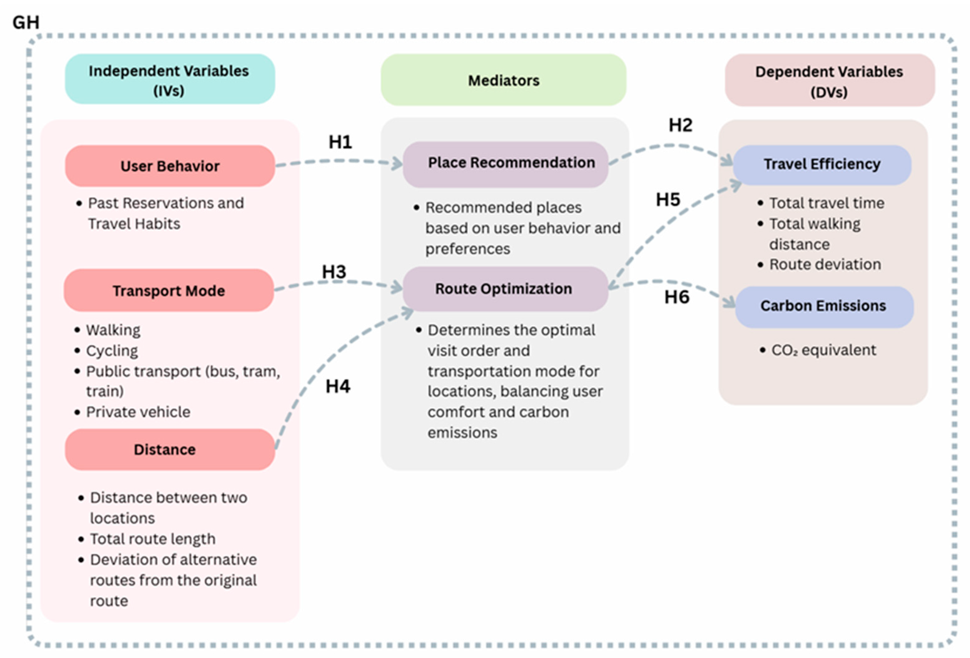
A hypothesis diagram linking the independent variables to dependent variables in the proposed object model is presented in Figure 3.
Figure 3 presents the general hypothesis (GH) as well as the hypotheses (H) that describe the relationships between the dependent and independent variables. These hypotheses are explained in detail below.
GH. 
A recommendation system that incorporates user behavior, transport mode, and distance—combined with effective route optimization—simultaneously improves travel efficiency and reduces carbon emissions.
H1. 
User behavior and past travel habits positively influence the relevance and accuracy of place recommendations.
H2. 
More accurate place recommendations improve travel efficiency by reducing unnecessary detours and planning effort.
H3. 
The selected transport mode significantly influences route optimization by constraining feasible paths and travel speeds.
H4. 
The spatial distance between locations affects route optimization by shaping the ordering and structure of candidate routes.
H5. 
More optimized routes reduce carbon emissions by minimizing total travel distance and avoiding inefficient segments.
H6. 
Route optimization enhances travel efficiency by minimizing total travel time and reducing route deviation.

4. Implementation

4.1. Data Collection and Preprocessing

The data collection process begins with user interactions within the system, where reservation details are gathered through a .NET-based backend infrastructure and a React-based user interface. These data points include users’ travel preferences, historical travel behaviors, and preferred venues. All collected information is securely stored in MongoDB, leveraging its flexible schema design and high scalability. Each reservation entry contains attributes such as reservation ID, location name, and geographic coordinates (latitude and longitude). The system workflow initiates when a user submits reservation information via the application. As reservations are made, the user profile model is continuously refined, enabling the generation of more accurate and personalized recommendations.
Due to privacy and access constraints, only the reservation scenarios themselves were generated synthetically. A total of 120 distinct reservation scenarios were constructed using realistic distributions reflecting real-world behaviors such as hours of the day, weekday/weekend patterns, and holiday variations. However, all environmental attributes associated with these reservations—such as venue IDs, distances, travel durations,—were obtained directly from the Google Places API, ensuring that these components of the dataset are entirely based on real-world data. Through their combination, approximately 50,000 event-level data points were created. To expand the recommendation scope, an area within a 40 km radius from the reservation coordinates is scanned. Venue preferences and transport modes were assigned using controlled proportional methods aligned with real-world probability distributions, enabling representative user behavior patterns for testing the model. This hybrid approach—synthetic reservation events combined with real-place and distance data—provides safe and realistic environment for evaluating the model’s decision-making and optimization capabilities while fully preserving data privacy. The raw reservation data is then enriched using the Google Places API to create a more comprehensive dataset. Information including venue ratings, distances, and categories is combined with the collected reservation data to create the Place Recommendation Dataset, as shown in Figure 4. This integration significantly enhances the system’s recommendation accuracy, enabling it to suggest more suitable and environmentally conscious venues.
Data preprocessing and transformation are handled via an API developed with the Flask framework. This API performs several critical tasks, including periodic data updates, handling missing or inconsistent values, enforcing proper formatting, and preparing the final dataset for training the XGBoost model. Through this pipeline, the system ensures robust, clean, and structured data management, ultimately improving the accuracy and reliability of the recommendation engine.

4.2. Data Transformations

Time and Distance Translations: Some of the data include time and distance information in different formats. In order to standardize the data, time is expressed in minutes and distance in kilometers.
Mandatory Fields: Key travel attributes such as Distance, CO2, Time and the target variable Score are guaranteed to be present.
Missing Data: Missing numerical values are replaced with 0 to ensure the model does not misinterpret absent data as padding and to prevent performance degradation, especially for attributes such as CO2 emissions or distance when they are unavailable.
Categorical Encoding: The Travel Mode categorical attribute is converted into numeric labels using LabelEncoder, with 0 reserved for padding.
Padding: Because the sequence lengths are different, all groups are padded to max_len. For numeric inputs, PAD_VAL_NUM = −999.0, and this value is defined as the mask_value in the Masking layer.
Scaling: StandardScaler is only fitted to non-mask (real) time steps. Therefore, pad values are not included in the scaling.
Data Control and Validation: In this process, automated with Flask API, data is regularly checked and validated. When a certain number of unique source coordinates are reached, this data is sent by API for route optimization purposes.

4.3. Route Data and LSTM Model Training

After preprocessing, step-level route information was generated using the Google Routes API, including travel distances, durations, and transportation mode-specific metrics for walking, bus, tram, and train segments. Each reservation was modeled as a sequential time series where each step represents an ordered movement within the sequence, and the normalized step index was included to capture the relative position of each movement. Because steps within a reservation are temporally and semantically dependent, sequence-wise training was applied with GroupKFold cross-validation to ensure that all steps from the same reservation remained in the same fold, preventing leakage between training and validation sets. This split effectively resulted in an 80% training set and a 20% validation set, ensuring performance evaluation on completely unseen reservation groups. A seed ensemble was employed to reduce variance arising from varying sequence lengths, while a batch size of 64 balanced contributions from short and long sequences, preventing short sequences from dominating the gradient updates. The model was trained for up to 100 epochs with EarlyStopping to halt training once validation loss stabilized, while ReduceLROnPlateau adjusted the learning rate dynamically to cope with sharp transitions in step scores, such as mode changes from walking to bus or tram. Gradient clipping further stabilized training on long sequences with consecutive high-duration steps, preventing exploding gradients and promoting smooth convergence. Collectively, these choices ensured that the LSTM could learn both short- and long-range dependencies in the sequences while maintaining numerical stability and generalization across diverse reservations. The components used in training the LSTM model are presented in Table 2. Table 2 presents the training strategies and process-specific hyperparameters used to enhance the LSTM model’s generalization ability and stability during the training process.

4.4. Proposed LSTM Model and XGBoost

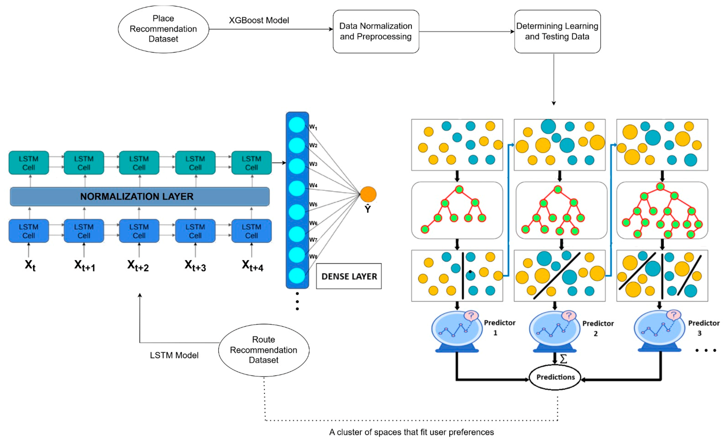
The XGBoost model is employed to generate personalized recommendations for places to visit within the context of a user’s reservation. The dataset is constructed using the geographic coordinates of the booking location alongside the reservation details provided by the user during registration. While reservation data initially serves to establish a preliminary user profile, it is progressively enriched with information derived from users’ past activities and behavioral patterns. In addition, the list of nodes that can be visited that we obtained from the Google Place API owing to the reservation locations of the users, the distance of these locations and the scores they received from other users are among the effective parameters in our data set. All these variables are analyzed by the model on a user basis and the suitability of each point that can be visited is scored for the user. These obtained scores constitute the main parameters that will help our model determine what route to follow in the LSTM phase. The results obtained from the XGBoost model consist of a set of locations for each reservation. These sets are processed by the system. The proposed model architecture is shown in Figure 4.
The proposed XGBoost model generates independent preference scores based on user-venue interaction for each candidate venue obtained from the Google Places API, providing route ranking input to the LSTM model. Instead of directly modeling sequential dependencies, the model evaluates the structural, locational, and contextual characteristics of each venue, combined with user information, to predict which places should be included in the route formation. By limiting the tree depth to a reasonable level, excessive splitting and memorization are prevented in this problem, where the number of observations per user is relatively limited, thus promoting a generalizable and simple decision structure. By keeping the learning rate low and using an early-stopping mechanism with numerous boosting rounds, the model ensures small and stable updates at each step; this design reduces instabilities arising from noisy or correlated features. By omitting L1 regularization and enabling L2 regularization in the regularization strategy, the unnecessary interactions of high-cardinality or high-variance variables such as Place_ID, category, and time are suppressed, helping the model to achieve a simple yet effective structure. The GroupKFold validation strategy prevents data leakage by providing group protection at the user level, enabling a more accurate measurement of the model’s true performance on a new user. Furthermore, by scaling features per fold, distance, time, and dummy variables are more consistent across histogram-based splits, supporting stable results with regularization. This integrated design allows XGBoost to be used as the primary component to capture user preferences without overfitting and provide reliable guidance for the LSTM’s route sorting task. The components used in training the XGBoost model are presented in Table 3.
The proposed LSTM model was designed using a two-layered sequence modeling approach, recognizing that step-by-step preferences within a reservation are sequential and context-aware rather than independent. Layer Normalization is applied to ensure features of heterogeneous scales are passed to the model with a balanced distribution, reducing internal training volatility. The two-layered LSTM stack provides the capacity to represent both local transitions and general trends observed across the entire reservation sequence. To constrain overfitting, Dropout and L2 regularization are applied, contributing to the learning of more generalized representations despite the variability in user and route data. The TimeDistributed layer at the output makes it possible for the model to produce a score specific to each step, while the Masked Huber loss maintains training integrity by excluding invalid padding time steps and offering a more stable error surface by limiting the influence of extreme outliers. The Adam optimizer was chosen for its ability to jointly optimize variable-scale features found in the reservation sequences, and maintaining a low learning rate ensures more stable convergence by preventing sudden deviations [40]. This integrated architecture allows the model to compactly and robustly learn the preference dynamics within route steps. Table 4 shows the details the architectural structure and fundamental training components utilized to ensure the proposed two-layered LSTM model efficiently learns the sequential preference dynamics within route steps.
The LSTM model evaluates the variety from each point A to point B and scores all available options according to factors such as transportation mode and distance that directly affect the carbon footprint and the reality of users’ ability to implement the route. These scores are valid for every point and variety that can be reached from point A. This result provides the optimal path for both environmental impact and user preference. It is often difficult to calculate and decide what is better for a user. In such cases, users may tend to prefer the shortest path. This model allows users to prefer routes with less carbon emissions without complicating their daily lives.
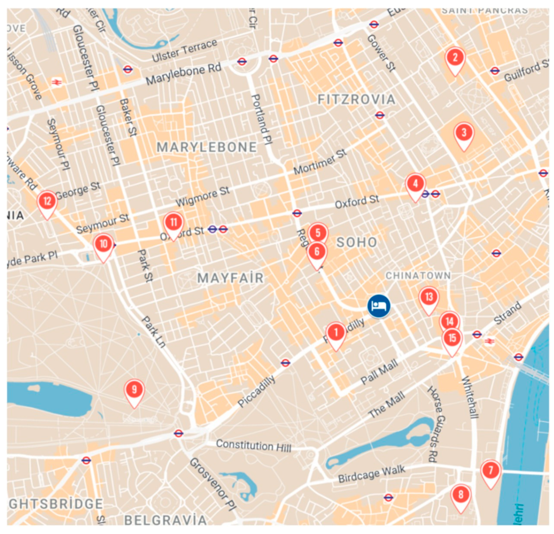
Figure 5 shows an example map of London, United Kingdom, with 15 different locations marked. The model is processed using a sample map by Google Route API. We assume 15 locations that can be visited according to the data provided by the XGBoost model. The pins consisting of numbers marked on the map indicate the order of the relevant location on the route. The starting point considers as the Housing location and route suggestions are adjusted to back to the Housing location. Firstly, in order to create a route with marked locations from 1 to 15, the starting and target points must be determined. The starting and target locations can be thought of as the matches of all locations on this map. For example, to go to another location from the place of accommodation, a location is selected from 15 location options. Similarly, the remaining 14 different options are evaluated to go to the next location. The selection of locations varies according to route, time, distance, and vehicle types. Therefore, location selections are directly related to carbon footprint when creating a route. After these steps are completed, a travel route with 15 locations is created.
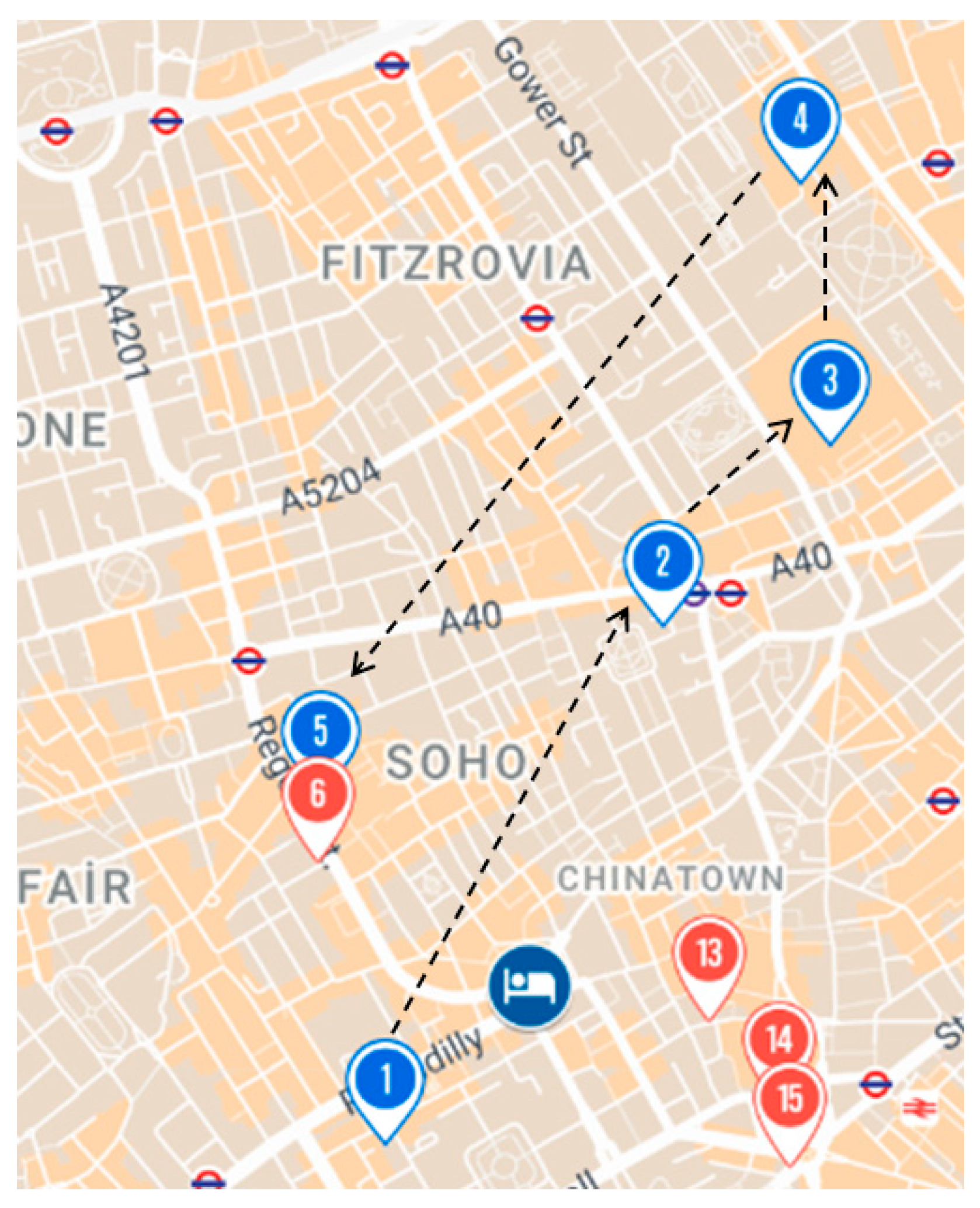
In the map shown in Figure 5, the locations visited from the Housing are determined sequentially. The route between these locations varies based on multiple parameters. Users generally prefer to visit locations that seem close to one another; however, this may not always represent the most optimal route. Factors such as available transportation options or public transit schedules may influence this behavior. This situation is illustrated in Figure 6 and Figure 7.
The algorithm makes a binary combination and decides on the next location. It reviews the time, distance and vehicle information between the locations specified in Table 5. Table 5 describes the route information shown in Figure 6.
The binary combination of each location creates many possibilities with route options and vehicle types. For this reason, a comparison is made between many locations to determine the first location to be visited from the reservation location. When creating a data set, instead of considering each row independently, it is necessary to create a data set where the next data is dependent on the previous data. At the same time, the interconnected rows should remember the previous situations in order for the route to be formed consistently. For this reason, using the LSTM model, which is a solution for time series, is a useful solution for our problem. In this way, the model has become able to learn long-term dependencies effectively. LSTM layers process consecutive time series data, rank the travel points suitable for the user’s interests, and optimize the transportation options between these points in terms of environmental effects and feasibility.
Figure 7 depicts an alternative route for the locations illustrated in Figure 6. The user prefers location 2, which is location 4 depicted in Figure 6, and ranks location 2 as location 4. The blue marks from 1 to 5 indicate the user’s preference order.
Table 6 shows that the route from location 1 to location 5 is completed in a longer distance and time compared to the route suggested by the model in Table 5. Although these differences seem insignificant to us, they cause an increase in carbon emissions throughout the travel. The route suggested by our algorithm has shown a much more effective and appropriate behavior in terms of both environmental impacts and user experience.

4.5. Comparison of Estimated and Actual Values

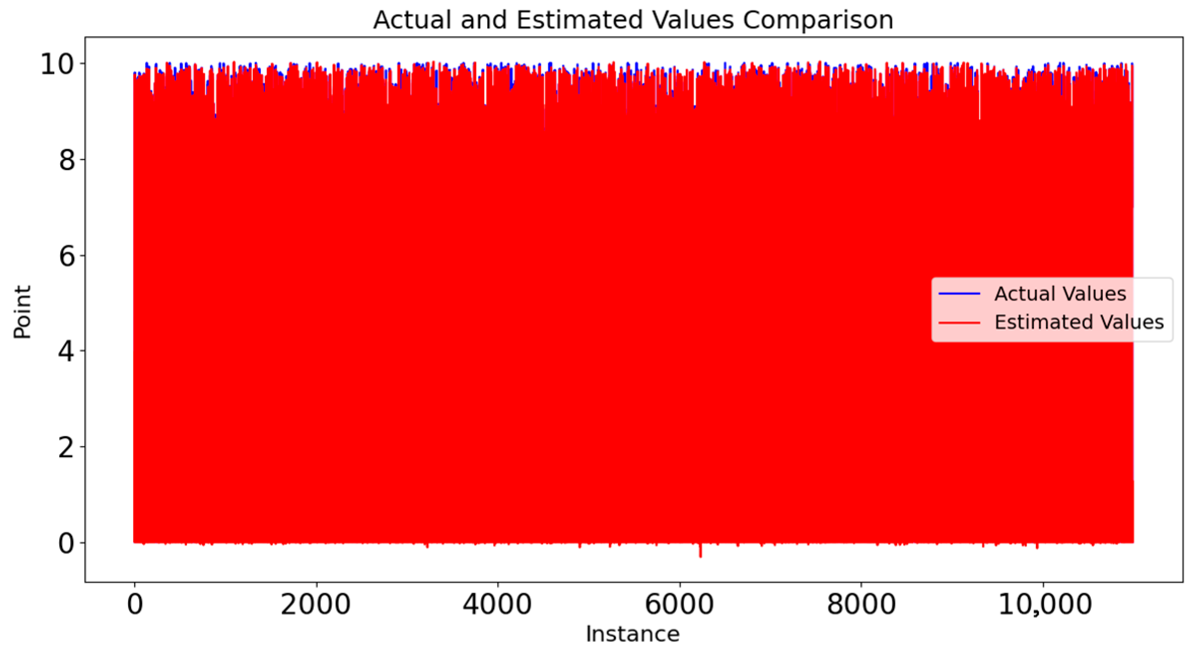
One of the most important methods for evaluating the success of deep learning models is to compare the values predicted by the model with the real values. The comparison of the scores predicted by the LSTM model with the real scores for each example in the test dataset is shown in Figure 8. Instance refers to each data point that the model predicted and represents one point for more than 10,000 different route predictions. The score is a measure that rates the reasonableness of going from a certain point to another. At each step, the model evaluates the most suitable destination from the current location, and the route with the highest score is preferred. In Figure 8, the X-axis shows the route predictions in the test dataset, and the Y-axis shows the scores assigned for these routes. The blue lines show how well the model matches the real scores, while the red lines represent the model’s predictions.
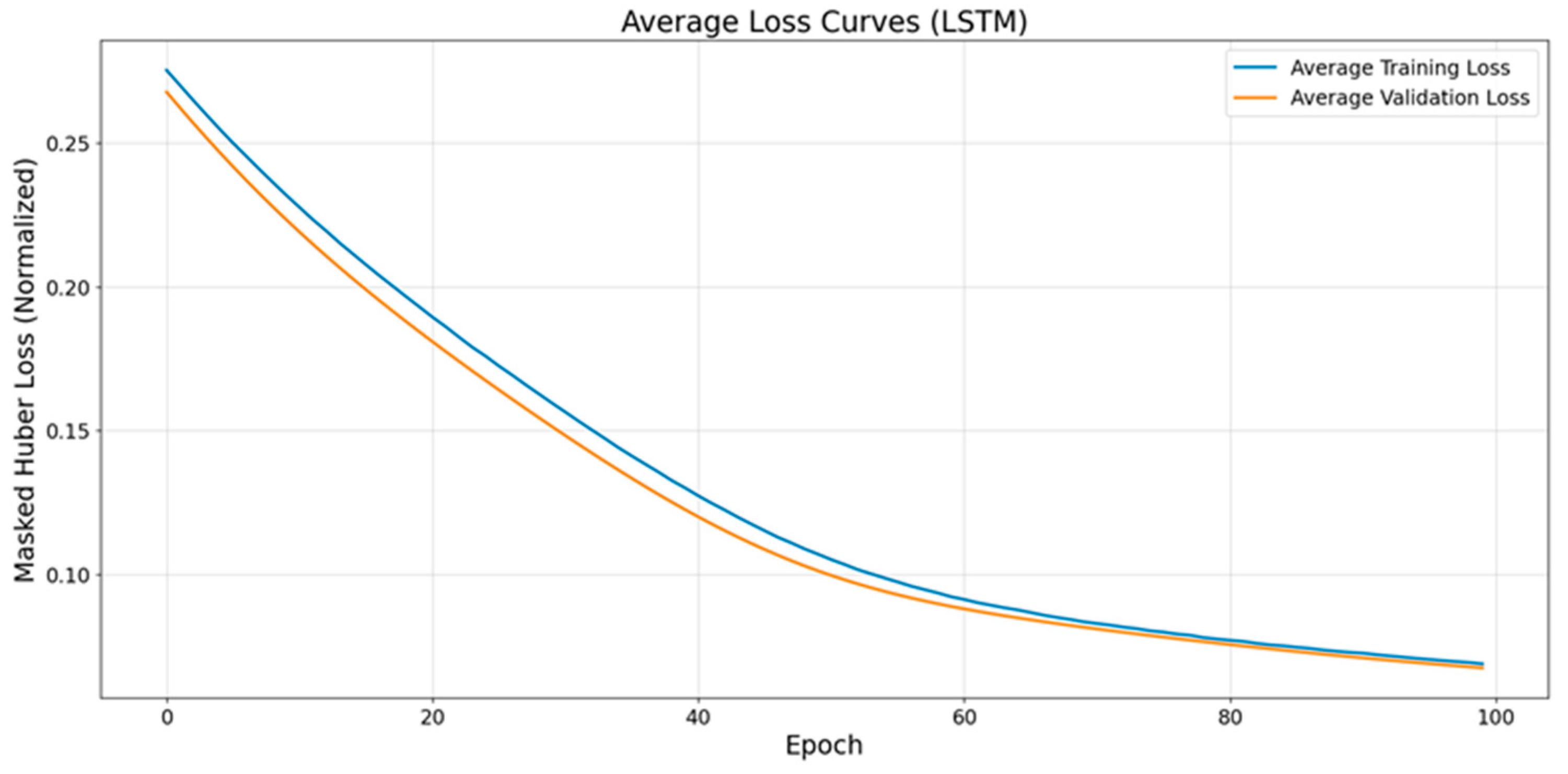
The average loss curves for LSTM is presented in Figure 9.
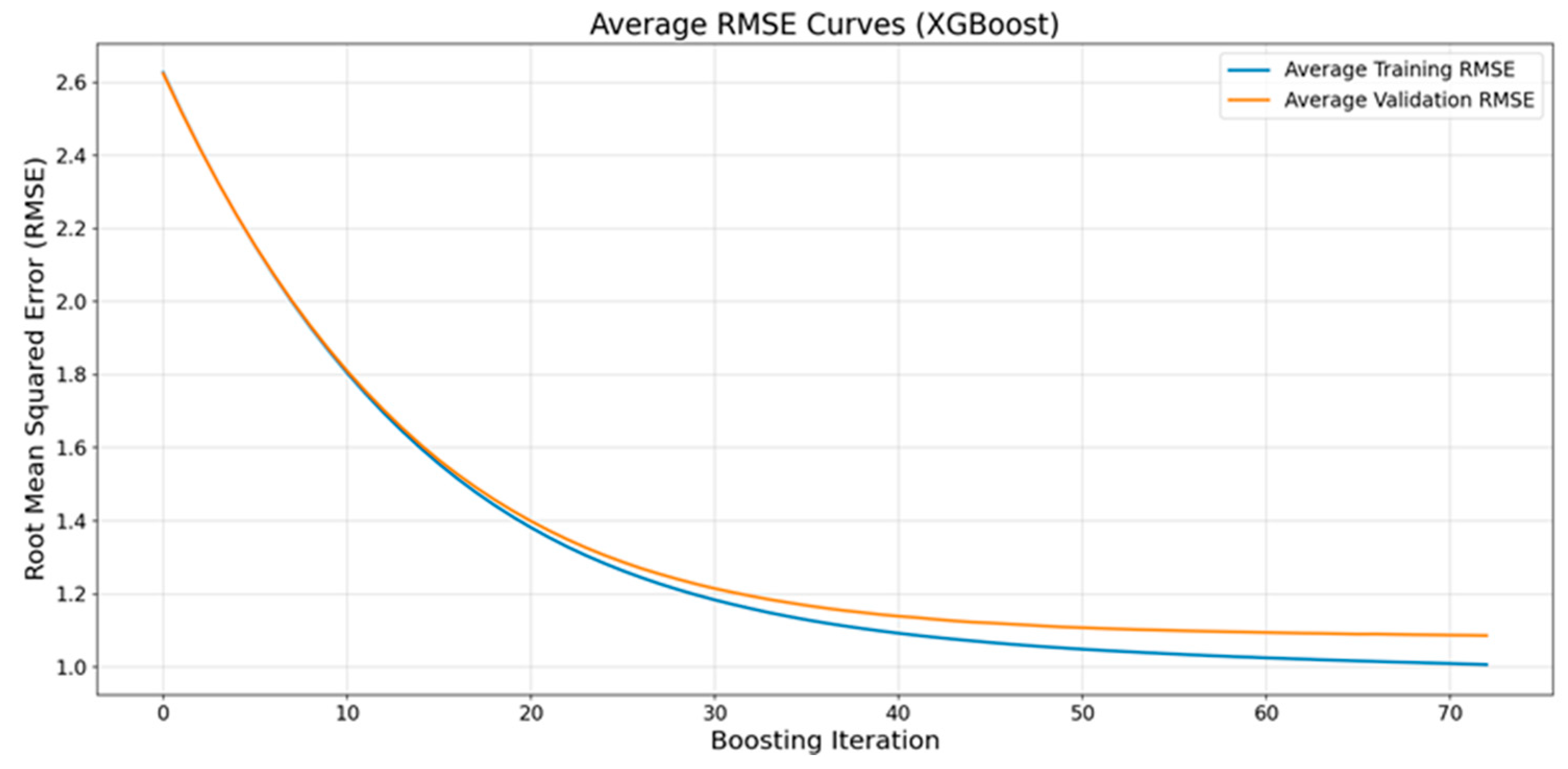
The average RMSE curves for XGBoost is presented in Figure 10.

4.6. Distribution of Forecast Errors

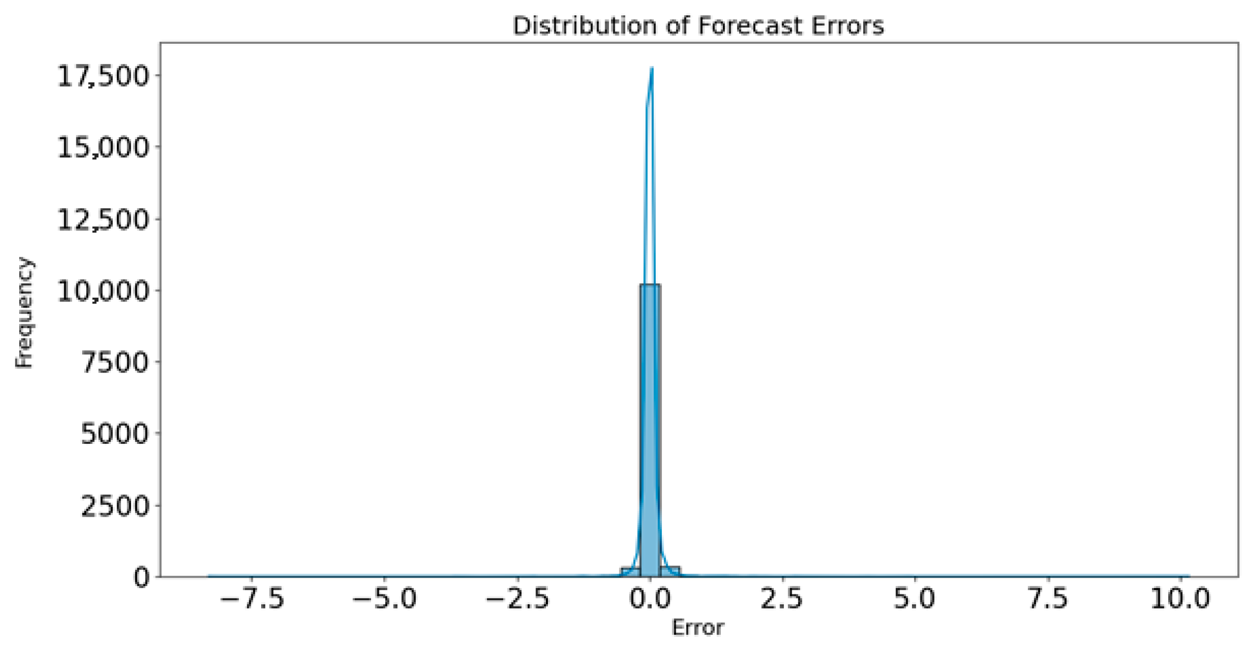
It is important to analyze the error levels with the accuracy of the model. The estimation error distribution of LSTM model is shown in Figure 11. Figure 11 shows KDE curve; this curve provides information about the error distribution by showing the smooth distribution of errors. The horizontal axis shows the differences between the real values and the estimated values (error). Positive errors indicate that the estimation is below the real value, while negative errors indicate that it is above. In this work, the horizontal axis represents the difference between the real and estimated scores given to the points on the route. The vertical axis indicates the frequency observed for each error value; this shows how much the model’s estimations are concentrated in certain error ranges. Figure 8 indicates that the LSTM model makes accurate estimations, as the estimation errors are symmetrical and concentrated around zero.

4.7. Statistical Analysis

For the LSTM analyses, folds were constructed based on individual reservations, and statistical comparisons were performed using reservation-level error values. To validate this approach, checks were conducted to assess potential user-induced dependencies. As a result, reservation-level observations were treated as independent, allowing the Wilcoxon signed-rank test to be applied. In contrast, for the XGBoost analyses, folds were assigned on a per-user basis, with all reservations of each user contained within a single fold. This design preserved independence between users, enabling the Wilcoxon test to be confidently applied to user-level error values. Across both model evaluations, the results include the Shapiro–Wilk normality test, the nonparametric Wilcoxon test (suitable for the small number of folds), bootstrap-derived 95% confidence intervals, and relevant effect size measures. Table 7 shows the statistical significance tests results for the LSTM and XGBoost models.
The Wilcoxon signed-rank test indicates that the RMSE difference between the LSTM and Ridge models is statistically significant, with the LSTM model achieving substantially lower RMSE values. And the MAE difference between the LSTM and Ridge models is statistically significant, with the LSTM model achieving substantially lower MAE values. The RMSE difference between the XGBoost and Linear Regression baseline is statistically significant, with the XGBoost model achieving substantially lower RMSE values. And the MAE difference between XGBoost and Linear Regression baseline is statistically significant, with the XGBoost model achieving substantially lower MAE values.

4.8. Distribution of Futures

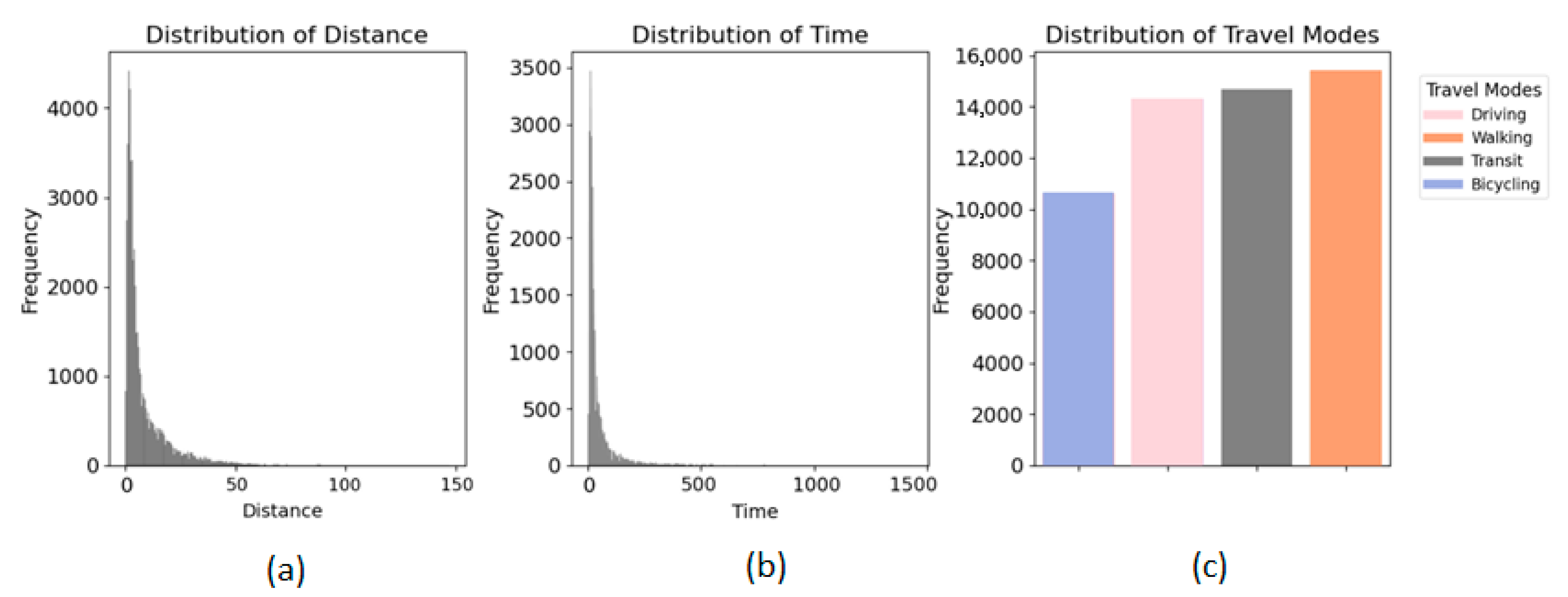
Figure 12 shows the distributions of three different features: distance, time, and travel mode. These features reveal the structure of the data features that the model takes into account when making predictions. The concentration areas in the distance and time variables indicate that the model encounters such data more frequently and can be more successful in predictions in these areas. Figure 12a shows the frequency of distances and which distance intervals are more common. Figure 12b shows how the time intervals are distributed and which durations are more common. Figure 12c shows how frequently different travel modes are used, and the frequencies of the modes expressed in numerical categories. These distributions help us understand the distribution and density of each feature in the dataset. Thus, it allows us to better analyze the structure of the data used in training the model.

5. Performance Metrics

In this work, four evolution metrics are used to compare the TRP model performance with other algorithms. The following equations define these metrics, respectively [41].
R M S E = 1 N   i = 1 N ( P i A i ) 2
M A E = 1 N   i = 1 N P i A i
M S E = 1 N   i = 1 N ( P r e d i c t e d i A c t u a l i ) 2
N R M S E = R M S E A m a x A m i n
where P and A denote predicted and actual values. N corresponds to number of samples.

5.1. Comparison of XGBoost and Other Algorithms

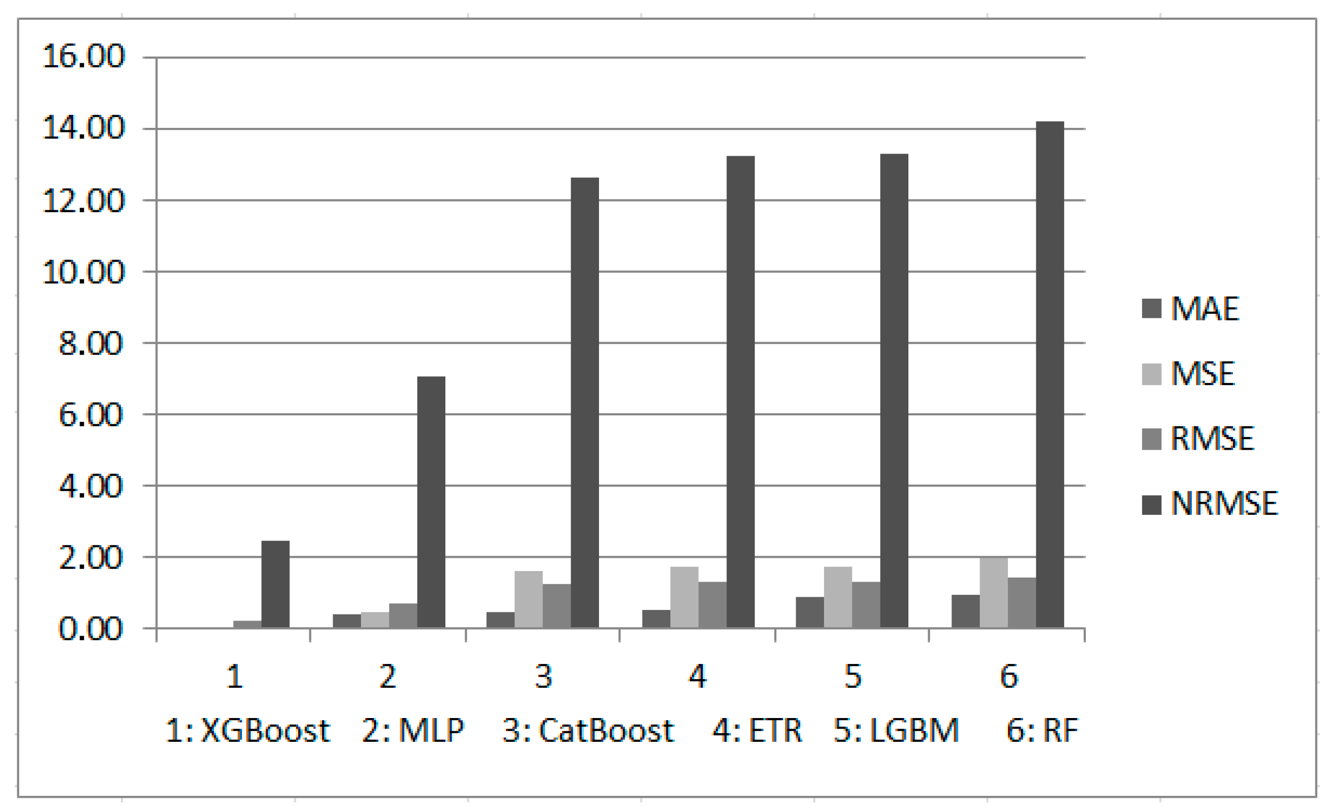
The XGBoost algorithm is particularly powerful in medium and large datasets and in modeling complex and nonlinear relationships. We define our dataset as medium and complex structure since it has multiple locations for each user and multiple features for each location. A scoring system has been developed that takes into account all the parameters to determine the most suitable locations for users. This system evaluates the suitability of each location from the user’s perspective. A lower score indicates that the location is less suitable for the user, while a higher score indicates a better option. Therefore, the estimation process in our algorithm aims to directly calculate and evaluate these scores. In addition to XGBoost algorithm, other algorithms are proposed for the TRP model performance. The algorithms that can be applied to the dataset and system structure are, respectively: MLP, ETR, LightGBM, CatBoost and RF algorithms. The error measurements of the algorithms are given comparatively in Table 8.
In Figure 13, the bar plots depicts the error measurements of the models.
The descriptions of the algorithms compared with XGBoost are presented below.
  • MLP is a type of artificial neural network consisting of input, hidden, and output layers that can learn nonlinear models. Activation functions are typically used in the hidden layers, while the output layer does not use them. MLPs are trained using the backpropagation method and work with loss functions such as mean squared error. They provide an effective solution for applications requiring multiple outputs [42,43].
  • RF is a method used in classification and regression problems. It creates multiple decision trees and combines their results to make the final decision. At each split, random features are selected, which helps reduce variance. It can work with both categorical and continuous data and provides effective results even in cases of missing or corrupted data. Additionally, it can be successfully applied to complex datasets with many variables [42,44].
  • ETR is an algorithm consisting of multiple decision trees that operates on the entire training data. The trees are constructed by selecting random subsets of features and split points. This approach increases generalization performance by ensuring independence and delivers successful results in both classification and regression problems [45].
  • LightGBM is a histogram-based algorithm that can handle categorical features and provides fast training time with low resource usage. The decision trees are split based on leaf information, which leads to lower loss and better results compared to other algorithms in terms of accuracy. Moreover, it is an optimized algorithm that works effectively with large datasets [46].
  • CatBoost is an algorithm which quickly processes categorical data by using the GBDT algorithm. It can achieve effective results even with limited data compared to deep learning models. This algorithm improves performance by working with categorical features during the training process, rather than during preprocessing as in traditional GBDT. Additionally, it uses special methods to prevent overfitting and prediction bias, improving prediction accuracy [47].

5.2. Comparison of LSTM and Other Algorithms

In this work, LSTM model proposes to users personalized travel routes. This model analyzes the time dependencies and historical data to recommend the most optimal routes by determining the sequence and mode of transport for each travel destination. Therefore, both user-friendly and environmentally friendly routes can be designed. LSTM enables more accurate predictions of future actions and transport options by effectively recalling past information. The scoring system is applied to evaluate routes based on their suitability for users and their low CO2 emissions. A higher score indicates a route that is more suitable for the user’s needs and environmentally friendly, while a lower score reflects a less suitable route. The comparison of error measurements with RNN and GRU are presented in Table 9.
In Figure 14, the bar plots depicts the error measurements of deep learning models.
RNN is a type of artificial neural network designed to process sequential data. These networks learn dependencies over time through hidden states by retaining information derived from previous inputs. The structure of RNNs consists of an input layer, a hidden layer, and an output layer. Unlike feedforward neural networks, RNNs contain recurrent connections, which allow information to be processed cyclically within the network. GRU addresses the vanishing gradient problem in RNNs and is ideal for processing time-series data. It controls the forgetting of past information and updates the cell state through reset and update gates. Due to its simple architecture, GRU has low computational costs and offers high performance during training. By eliminating the vanishing gradient problem, GRU provides a robust method for time-series analysis [48,49,50].

6. Impact of TRP on Carbon Emission

Carbon emissions are classified in two ways as direct and indirect emissions according to the ISO 14040:2006 standard [51] and the Greenhouse Gas Protocol [52,53]. This study examines only the directly occurring carbon emissions. The Tier-1 methodology recommended by the Intergovernmental Panel on Climate Change (IPCC) is used for emission calculations [54]. The energy contents of fuels are calculated by multiplying the fuel consumption data with the conversion coefficients specified in the IPCC guide. These coefficients are determined by the Communiqué on Monitoring and Reporting of Greenhouse Gas Emissions published in the Official Gazette dated 22 July 2014 and numbered 29,068, and are also the data included in the IPCC 2006 Guide. Table 10 shows the parameters of fuel type [55,56,57].
In the Tier-1 approach, calculations are based on fuel consumption. In this method, the amount of emissions is determined depending on the amount of fuel used. Calculations are made based on the amount of consumption according to the type of fuel and only the default conversion factors. It is assumed that the average fuel consumption is 7.3 L per 100 km by car and 29.9 L by bus [58]. Accordingly, the total fuel consumption per person is calculated assuming that users visit all locations on their route. The first step in calculating CO2 emissions is to determine the amount of energy consumption. Fuel consumption values (tons) are calculated in Equation (9) according to fuel types. Then, these values are multiplied by the net calorie (TJ/kt) values to calculate the energy amount of the fuel (TJ).
Energy consumption [TJ] = Fuel consumption [t] × Conversion factor [TJ/kt]
The carbon content of the consumed fuel is determined by Equation (10). In this process, the energy factor is multiplied by the carbon emission factor, which is expressed in the unit of TJ of carbon content per ton of energy. The resulting carbon content is converted to the unit Gg specified in Equation (11) by scaling it by 10−3.
Carbon content [t C] = Carbon emission factor [t C/TJ] × Energy consumption [TJ]
Carbon   content   [ Gg   C ] = Carbon   content   [ t   C ] × 10 3
The proportion of carbon that undergoes oxidation is calculated using Equation (12). This value is determined by multiplying the carbon oxidation rate by the carbon content.
Carbon emission [Gg C] = Carbon content [Gg C] × Carbon oxidation rate
Equation (13) is used in the calculation of CO2 emissions.
CO2 emission [Gg CO] = Carbon emission [Gg C] × (44/12)
The molar masses of carbon dioxide and carbon are given in Table 11. The calculated emission value is multiplied by the ratio of these molar masses to obtain the CO2 emission [59,60].
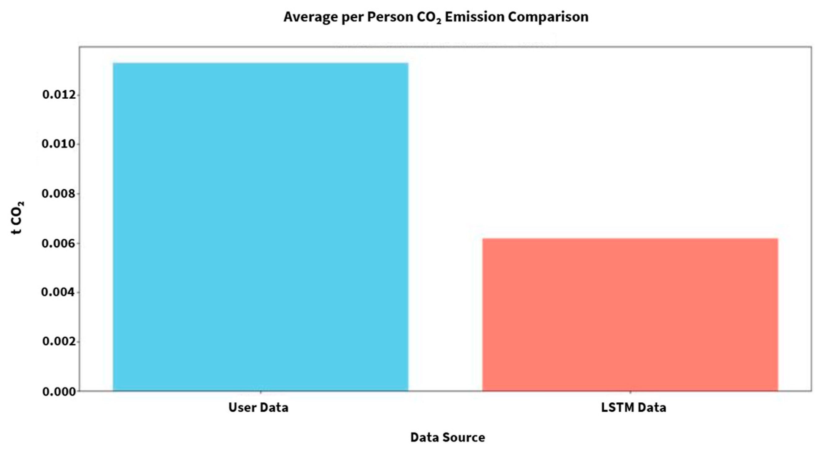
Calculations in Tier 1 management were performed using the suggestions we obtained from the LSTM model and the user data. In Figure 15, it is observed that the total carbon emission in the routes suggested by the LSTM model is approximately 53.46% less than the carbon emission per person in the travel routes selected by the users. This ratio may vary depending on the preferences of the users. However, users may not be able to calculate and analyze routes with different probabilities for multiple locations as detailed as the LSTM model. Thus, it is concluded that the LSTM model is more successful.
This study quantitatively evaluates the environmental impact of the proposed LSTM-based route recommendation algorithm by comparing its performance with two baseline models that reflect traditional user travel preferences. Because these baseline models do not include any CO2 optimization mechanisms, they function as control scenarios, highlighting the emission-reduction potential of the proposed algorithm.
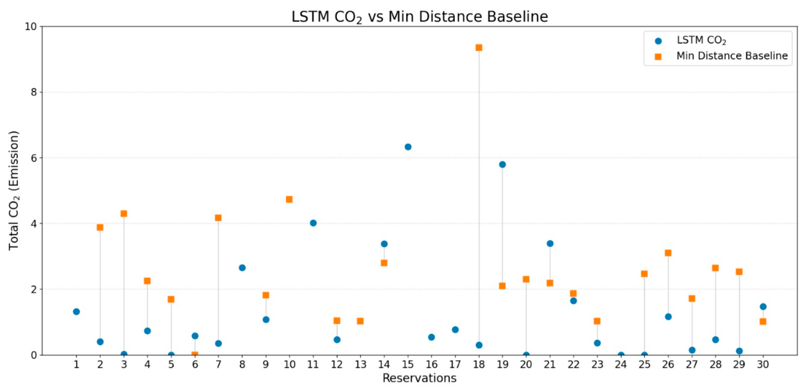
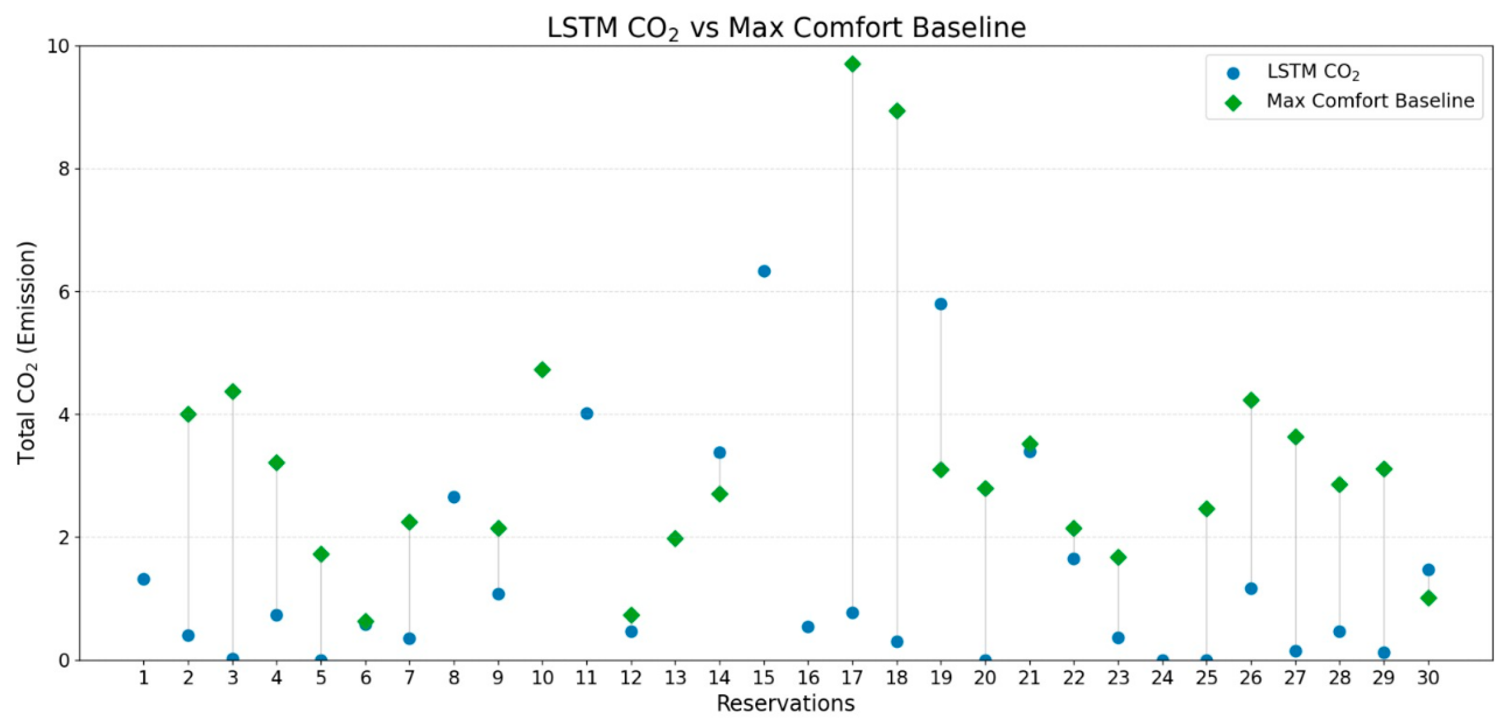
The analysis shows that the CO2 costs computed by the Min Distance Baseline (which selects the locally shortest path) generally exhibit higher values compared to those produced by the LSTM algorithm (Figure 16). This finding indicates that the algorithm implements a long-term, global emission-reduction strategy that goes beyond merely choosing short-distance routes and instead optimizes across the entire chain. Furthermore, the Max Comfort Baseline—defined as a proxy for user behavior by prioritizing highest comfort—was observed to generate notably high CO2 costs. The results demonstrate that the LSTM algorithm consistently yields lower CO2 emission outputs compared to both baseline scenarios (Figure 17). This provides strong evidence supporting the hypothesis that the algorithm can deliver environmental efficiency even in scenarios that resemble users’ conventional choices.

7. Conclusions and Discussion

This study presents an innovative travel recommendation system that prioritizes sustainability by integrating environmental factors, such as carbon footprint, into travel planning. By leveraging the LSTM and XGBoost models, the system generates personalized, optimized travel routes and suggests low-carbon transportation modes and environmentally friendly activities. Compared to traditional reservation systems, which focus primarily on price, duration, or popularity, the proposed approach encourages conscious travel decisions, supports local businesses, and promotes cultural engagement. User-generated data, including reservation details, travel preferences, and historical behaviors form the foundation of the dataset, which is further enriched with external information such as venue ratings, distances, and categories obtained via the Google Places API. Analyses of user behavior reveal that individuals often prioritize personal comfort over environmental considerations, highlighting the value of AI-driven guidance in fostering sustainable travel choices. The interactive mapping interface and spatial decision-support mechanisms enhance user engagement, enabling the creation of feasible, personalized itineraries. The experimental results further demonstrate that routes suggested by the LSTM model differ from typical user preferences, achieving improvements in both time efficiency and environmental impact. Overall, this study provides a practical tool for environmentally responsible travel, demonstrating that integrating AI-driven recommendations with sustainability criteria can effectively reduce carbon emissions, optimize travel planning, and promote meaningful, culturally rich travel experiences.
Future work could focus on integrating real-time traffic and weather data with detailed energy consumption measurements to enhance the carbon reduction effectiveness of an AI-based route recommendation system. The system’s route planning could be further improved by adapting to dynamic variables such as traffic density, road closures, and weather conditions. Parameters such as vehicle type, speed, and road gradients could be measured through sensors and advanced data collection techniques, enabling far more accurate carbon emission estimates. With a comprehensive data-collection and analysis approach, AI would not only optimize distance or travel time but also strengthen environmental sustainability indicators by accounting for dynamic conditions.

Author Contributions

Conceptualization, G.I. and Y.G.; methodology, S.E.; software, G.I. and Y.G.; validation, G.I. and Y.G.; formal analysis, G.I. and Y.G.; investigation, S.E.; resources, G.I. and Y.G.; data curation, G.I. and Y.G.; writing—original draft preparation, G.I., Y.G. and S.E.; writing—review and editing, S.E.; visualization, G.I. and Y.G. All authors have read and agreed to the published version of the manuscript.

Funding

This research received no external funding.

Institutional Review Board Statement

Not applicable.

Informed Consent Statement

Not applicable.

Data Availability Statement

The raw data supporting the conclusions of this article will be made available by the authors on request.

Conflicts of Interest

The authors declare no conflicts of interest.

Abbreviations

The following abbreviations are used in this manuscript:
AIArtificial Intelligence
CatBoostCategorical Boosting
CO2Carbon dioxide
ETRExtra Trees Regressor
GBDTGradient Boosting Decision Tree
GgGigagram
GHGsGreenhouse Gas emissions
GRUGated Recurrent Unit
GtCO2eGigatons of CO2 equivalent
KDEKernel Density Estimation
LightGBMLight Gradient Boosting Machine
LSTM Long Short-Term Memory
MAEMean Absolute Error
MLPMulti-Layer Perception
MSEMean Squared Error
NRMSENormalized Root Mean Square Error
RFRandom Forest
RMSERoot Mean Square Error
RNNRecurrent Neural Networks
TRPTravel Route Planning
XGBoost Extreme Gradient Boosting

References

  1. Sadollah, A.; Nasir, M.; Geem, Z.W. Sustainability and Optimization: From Conceptual Fundamentals to Applications. Sustainability 2020, 12, 2027. [Google Scholar] [CrossRef]
  2. Bouakkaz, A.; Mena, A.J.G.; Haddad, S.; Ferrari, M.L. Efficient Energy Scheduling Considering Cost Reduction and Energy Saving in Hybrid Energy System with Energy Storage. J. Energy Storage 2021, 33, 101887. [Google Scholar] [CrossRef]
  3. Sylejmani, K.; Abdurrahmani, V.; Ahmeti, A.; Gashi, E. Solving the Tourist Trip Planning Problem with Attraction Patterns Using Meta-Heuristic Techniques. Inf. Technol. Tour. 2024, 26, 633–678. [Google Scholar] [CrossRef]
  4. Schmitz, M.F.; Rodriquez, P.D. Tourism as a Challenge; WIT Series on Tourism Today; WIT Press: Southampton, UK, 2014. [Google Scholar]
  5. Aribas, E.; Daglarli, E. Transforming Personalized Travel Recommendations: Integrating Generative AI with Personality Models. Electronics 2024, 13, 4751. [Google Scholar] [CrossRef]
  6. United Nations Environment Programme (UNEP). Emissions Gap Report 2024: No More Hot Air … Please! With a Massive Gap between Rhetoric and Reality, Countries Draft New Climate Commitments; UNEP: Nairobi, Kenya, 2024; Available online: https://wedocs.unep.org/20.500.11822/46404 (accessed on 23 October 2025).
  7. Lenzen, M.; Sun, Y.-Y.; Faturay, F.; Ting, Y.-P.; Geschke, A.; Malik, A. The Carbon Footprint of Global Tourism. Nat. Clim. Change 2018, 8, 522–528. [Google Scholar] [CrossRef]
  8. World Tourism Organization; International Transport Forum. Transport-Related CO2 Emissions of the Tourism Sector–Modelling Results; UNWTO: Madrid, Spain, 2019. [Google Scholar] [CrossRef]
  9. Corbeil, J.-P.; Daudens, F. Deploying a Cost-Effective and Production-Ready Deep News Recommender System in the Media Crisis Context. In Proceedings of the ORSUM@ACM RecSys 2020, Rio de Janeiro, Brazil, 25 September 2020. Virtual Event. [Google Scholar]
  10. Yao, H.; Liu, Y.; Zhang, X. Developing Deep LSTM Model for Real-Time Path Planning in Unknown Environments. In Proceedings of the 7th International Conference on Dependable Systems and Their Applications (DSA), Xi’an, China, 28–29 November 2020; pp. 219–225. [Google Scholar] [CrossRef]
  11. Chen, X.; Zhang, H.; Xiao, F.; Peng, D.; Zhang, C.; Hong, B. Route Planning by Merging Local Edges into Domains with LSTM. In Proceedings of the 2022 IEEE 25th International Conference on Intelligent Transportation Systems (ITSC), Macau, China, 8–12 October 2022; pp. 505–510. [Google Scholar] [CrossRef]
  12. Zhang, Y.; Chen, P. Path Planning of a Mobile Robot for a Dynamic Indoor Environment Based on an SAC-LSTM Algorithm. Sensors 2023, 23, 9802. [Google Scholar] [CrossRef]
  13. Park, K.-W.; Kim, M.; Kim, J.-S.; Park, J.-H. Path Planning for Multi-Arm Manipulators Using Soft Actor–Critic Algorithm with Position Prediction of Moving Obstacles via LSTM. Appl. Sci. 2022, 12, 9837. [Google Scholar] [CrossRef]
  14. Kong, J.; Huang, J.; Yu, H.; Deng, H.; Gong, J.; Chen, H. RNN-Based Default Logic for Route Planning in Urban Environments. Neurocomputing 2019, 338, 307–320. [Google Scholar] [CrossRef]
  15. Hoang, N.-T.; Tong, V.; Tran, H.A.; Duong, C.S.; Nguyen, T.L.T. LSTM-Based Server and Route Selection in Distributed and Heterogeneous SDN Network. J. Comput. Sci. Cybern. 2023, 39, 79–99. [Google Scholar] [CrossRef]
  16. Sanagavarapu, S.; Sridhar, S. SDPredictNet—A Topology-Based SDN Neural Routing Framework with Traffic Prediction Analysis. In Proceedings of the 2021 IEEE 11th Annual Computing and Communication Workshop and Conference (CCWC), Las Vegas, NV, USA, 27–30 January 2021; pp. 264–272. [Google Scholar]
  17. Azzouni, A.; Boutaba, R.; Pujolle, G. Neuroute: Predictive Dynamic Routing for Software-Defined Networks. In Proceedings of the 2017 13th International Conference on Network and Service Management (CNSM), Tokyo, Japan, 26–30 November 2017; pp. 1–6. [Google Scholar]
  18. Sun, G.; Li, T. Optimizing Logistics in Forestry Supply Chains: A Vehicle Routing Problem Based on Carbon Emission Reduction. Forests 2025, 16, 62. [Google Scholar] [CrossRef]
  19. Mohsen, B.M. AI-Driven Optimization of Urban Logistics in Smart Cities: Integrating Autonomous Vehicles and IoT for Efficient Delivery Systems. Sustainability 2024, 16, 11265. [Google Scholar] [CrossRef]
  20. Xu, Z.; Zheng, C.; Zheng, S.; Ma, G.; Chen, Z. Multimodal Transportation Route Optimization of Emergency Supplies under Uncertain Conditions. Sustainability 2024, 16, 10905. [Google Scholar] [CrossRef]
  21. Li, L.; Zhang, Q.; Zhang, T.; Zou, Y.; Zhao, X. Optimum Route and Transport Mode Selection of Multimodal Transport with Time Window under Uncertain Conditions. Mathematics 2023, 11, 3244. [Google Scholar] [CrossRef]
  22. Yi, Z.; Bauer, P.H. Optimal Stochastic Eco-routing Solutions for Electric Vehicles. IEEE Trans. Intell. Transp. Syst. 2018, 19, 3807–3817. [Google Scholar] [CrossRef]
  23. Owais, M.; Alshehri, A. Pareto Optimal Path Generation Algorithm in Stochastic Transportation Networks. IEEE Access 2020, 8, 58970–58981. [Google Scholar] [CrossRef]
  24. Almutairi, A.; Owais, M. Reliable Vehicle Routing Problem Using Traffic Sensors Augmented Information. Sensors 2025, 25, 2262. [Google Scholar] [CrossRef]
  25. Champahom, T.; Banyong, C.; Janhuaton, T.; Se, C.; Watcharamaisakul, F.; Ratanavaraha, V.; Jomnonkwao, S. Deep Learning vs. Gradient Boosting: Optimizing Transport Energy Forecasts in Thailand Through LSTM and XGBoost. Energies 2025, 18, 1685. [Google Scholar] [CrossRef]
  26. Mazibuko, T.; Akindeji, K. Hybrid Forecasting for Energy Consumption in South Africa: LSTM and XGBoost Approach. Energies 2025, 18, 4285. [Google Scholar] [CrossRef]
  27. Çınarer, G.; Yeşilyurt, M.K.; Ağbulut, Ü.; Yılbaşı, Z.; Kılıç, K. Application of various machine learning algorithms in view of predicting the CO2 emissions in the transportation sector. Sci. Technol. Energy Transit. 2024, 79, 15. [Google Scholar] [CrossRef]
  28. IPCC. Global Warming of 1.5 °C; Masson-Delmotte, V., Zhai, P., Pörtner, H.-O., Roberts, D., Skea, J., Shukla, P.R., Pirani, A., Moufouma-Okia, W., Péan, C., Pidcock, R., et al., Eds.; Cambridge University Press: Cambridge, UK; New York, NY, USA, 2018; pp. 3–24. [Google Scholar] [CrossRef]
  29. World Health Organization (WHO). Climate Change, October 2023. Available online: https://www.who.int/news-room/fact-sheets/detail/climate-change-and-health (accessed on 23 October 2025).
  30. Singer, M. Climate Change and Social Inequality: The Health and Social Costs of Global Warming; Routledge: New York, NY, USA, 2018; Volume 152, pp. 1–247. [Google Scholar]
  31. Diffenbaugh, N.S.; Burke, M. Global Warming Has Increased Global Economic Inequality. Proc. Natl. Acad. Sci. USA 2019, 116, 9808–9813. [Google Scholar] [CrossRef]
  32. Hochreiter, S.; Schmidhuber, J. Long Short-Term Memory. Neural Comput. 1997, 9, 1735–1780. [Google Scholar] [CrossRef] [PubMed]
  33. Van Houdt, G.; Mosquera, C.; Nápoles, G. A Review on the Long Short-Term Memory Model. Artif. Intell. Rev. 2020, 53, 5929–5955. [Google Scholar] [CrossRef]
  34. Kaja, S.; Shakshuki, E.M.; Yasar, A. Long Short-Term Memory Approach for Routing Optimization in Cloud ACKnowledgement Scheme for Node Network. Procedia Comput. Sci. 2021, 184, 461–468. [Google Scholar] [CrossRef]
  35. Lindemann, B.; Müller, T.; Vietz, H.; Jazdi, N.; Weyrich, M. A Survey on Long Short-Term Memory Networks for Time Series Prediction. Procedia CIRP 2021, 99, 650–655. [Google Scholar] [CrossRef]
  36. Tsai, C.-Y.; Tai, L.-Y.; Lo, C.-C. An LSTM-Based Personalized Travel Route Recommendation System. In Proceedings of the 2023 Congress in Computer Science, Computer Engineering, & Applied Computing (CSCE), Las Vegas, NV, USA, 24–27 July 2023. [Google Scholar]
  37. Siddiqui, J.; Ahmed, U.; Amin, A.; Alharbi, T.; Alharbi, A.; Aziz, I.; Khan, A.R.; Mahmood, A. Electric Vehicle Charging Station Load Forecasting with an Integrated DeepBoost Approach. Alex. Eng. J. 2025, 116, 331–341. [Google Scholar] [CrossRef]
  38. Ding, H. Establishing a soil carbon flux monitoring system based on support vector machine and XGBoost. Soft Comput. 2024, 28, 1–24. [Google Scholar] [CrossRef]
  39. Palermo, J. The Onion Architecture: Part 1. Jeffrey Palermo Blog 2008. Available online: https://jeffreypalermo.com/2008/07/the-onion-architecture-part-1/ (accessed on 23 October 2025).
  40. Sun, H.; Zhou, W.; Shao, Y.; Cui, J.; Xing, L.; Zhao, Q.; Zhang, L. A Linear Interpolation and Curvature-Controlled Gradient Optimization Strategy Based on Adam. Algorithms 2024, 17, 185. [Google Scholar] [CrossRef]
  41. Sharma, D.K.; Chatterjee, M.; Kaur, G.; Vavilala, S. Deep Learning Applications for Disease Diagnosis. In Deep Learning for Medical Applications with Unique Data; Gupta, D., Kose, U., Khanna, A., Balas, V.E., Eds.; Academic Press: Cambridge, MA, USA, 2022; pp. 31–51. [Google Scholar]
  42. Kurt, N.; Ozturk, O.; Beken, M. Estimation of Gas Emission Values on Highways in Turkey with Machine Learning. In Proceedings of the 2021 10th International Conference on Renewable Energy Research and Applications (ICRERA), Istanbul, Turkey, 26–29 September 2021; pp. 443–446. [Google Scholar] [CrossRef]
  43. Colak, M.; Yesilbudak, M.; Bayindir, R. Forecasting of Daily Total Horizontal Solar Radiation Using Grey Wolf Optimizer and Multilayer Perceptron Algorithms. In Proceedings of the 2019 8th International Conference on Renewable Energy Research and Applications (ICRERA), Brasov, Romania, 3–6 November 2019; pp. 939–942. [Google Scholar] [CrossRef]
  44. Breiman, L. Random Forests. Mach. Learn. 2001, 45, 5–32. [Google Scholar] [CrossRef]
  45. Aziz, T.; Camana, M.R.; Garcia, C.E.; Hwang, T.; Koo, I. REM-Based Indoor Localization with an Extra-Trees Regressor. Electronics 2023, 12, 4350. [Google Scholar] [CrossRef]
  46. Cai, Z.; Huang, H.; Sun, G.; Li, Z.; Ouyang, C. Advancing Predictive Models: Unveiling LightGBM Machine Learning for Data Analysis. In Proceedings of the 2023 4th International Conference on Computer, Big Data and Artificial Intelligence (ICCBD+AI), Guiyang, China, 15–17 December 2023; pp. 109–112. [Google Scholar] [CrossRef]
  47. Kumar, G.S.; Dhanalakshmi, R. Performance Analysis of CatBoost Algorithm and XGBoost Algorithm for Prediction of CO2 Emission Rating. In Proceedings of the 2023 6th International Conference on Contemporary Computing and Informatics (IC3I), Gautam Buddha Nagar, India, 14–16 December 2023; pp. 1497–1501. [Google Scholar] [CrossRef]
  48. Liu, L.; Li, C.; Li, X.; Ge, Q. State of Energy Estimation of Electric Vehicle Based on GRU-RNN. In Proceedings of the 2022 37th Youth Academic Annual Conference of Chinese Association of Automation (YAC), Beijing, China, 19–20 November 2022; pp. 115–120. [Google Scholar] [CrossRef]
  49. Alshehri, O.S.; Alshehri, O.M.; Samma, H. Blood Glucose Prediction Using RNN, LSTM, and GRU: A Comparative Study. In Proceedings of the 2024 IEEE International Conference on Advanced Systems and Emergent Technologies (IC_ASET), Hammamet, Tunisia, 27–29 April 2024; pp. 1–5. [Google Scholar] [CrossRef]
  50. Routray, N.; Rout, S.K.; Sahu, B. Breast Cancer Prediction Using Deep Learning Technique RNN and GRU. In Proceedings of the 2022 Second International Conference on Computer Science, Engineering and Applications (ICCSEA), Gunupur, India, 8 September 2022; pp. 1–5. [Google Scholar] [CrossRef]
  51. ISO 14040:2006; Environmental Management—Life Cycle Assessment—Principles and Framework. International Organization for Standardization: Geneva, Switzerland, 2006.
  52. Weidema, B.P. Comparison of the Requirements of the GHG Protocol Product Life Cycle Standard and the ISO 14040 Series; 2.-0 LCA Consultants: Aalborg, Denmark, 2022. [Google Scholar]
  53. Bhatia, P.; Ranganathan, J.; World Business Council for Sustainable Development (WBCSD). The Greenhouse Gas Protocol: A Corporate Accounting and Reporting Standard, Revised Edition; World Resources Institute: Washington, DC, USA, 2004. [Google Scholar]
  54. Hünerli, E.; Karaca Dolgun, G.; Ural, T.; Güllüce, H.; Karabacak, D. Calculation of Muğla Sıtkı Koçman University’s Carbon Footprint with IPCC Tier 1 Approach and DEFRA Method. Kırklareli Univ. J. Eng. Sci. 2024, 10, 1–28. [Google Scholar] [CrossRef]
  55. Eggleston, H.S.; Buendia, L.; Miwa, K.; Ngara, T.; Tanabe, K. 2006 IPCC Guidelines for National Greenhouse Gas Inventories; Institute for Global Environmental Strategies (IGES): Hayama, Japan, 2006. [Google Scholar]
  56. Kardeş Selimoğlu, S.; Poroy Arsoy, A.; Bora Kılınçarslan, T. Creating Assurance on Greenhouse Gas Statements According to the International Assurance Standard 3410 within the Context of Elements of Assurance Engagement. J. Account. Financ. 2022, 21–34. [Google Scholar] [CrossRef]
  57. Kılıç, E.; Önler, E. A Study on the Calculation of the Carbon Footprint of Public Transport in Çorlu District of Tekirdağ Province. Eur. J. Sci. Technol. 2022, 41, 67–72. [Google Scholar]
  58. IPCC. Revised 1996 IPCC Guidelines for National Greenhouse Gas Inventories, Volume III: Reference Manual, Chapter 1: Energy; IPCC: Geneva, Switzerland, 1996. [Google Scholar]
  59. Kiliç, M.Y.; Dönmez, T.; Adalı, S. Change of Carbon Footprint Due to Fuel Consumption: Çanakkale Case Study. Gümüşhane Univ. J. Sci. Technol. 2021, 11, 943–955. [Google Scholar] [CrossRef]
  60. Kaplanseren, B.; Mercan, B.; Özdemir, B.; Kadıoğlu, H.H.; Sel, Ç. Carbon Footprint in Vehicle Routing and an Industrial Application. Int. J. Eng. Res. Dev. 2019, 11, 239–252. [Google Scholar] [CrossRef]
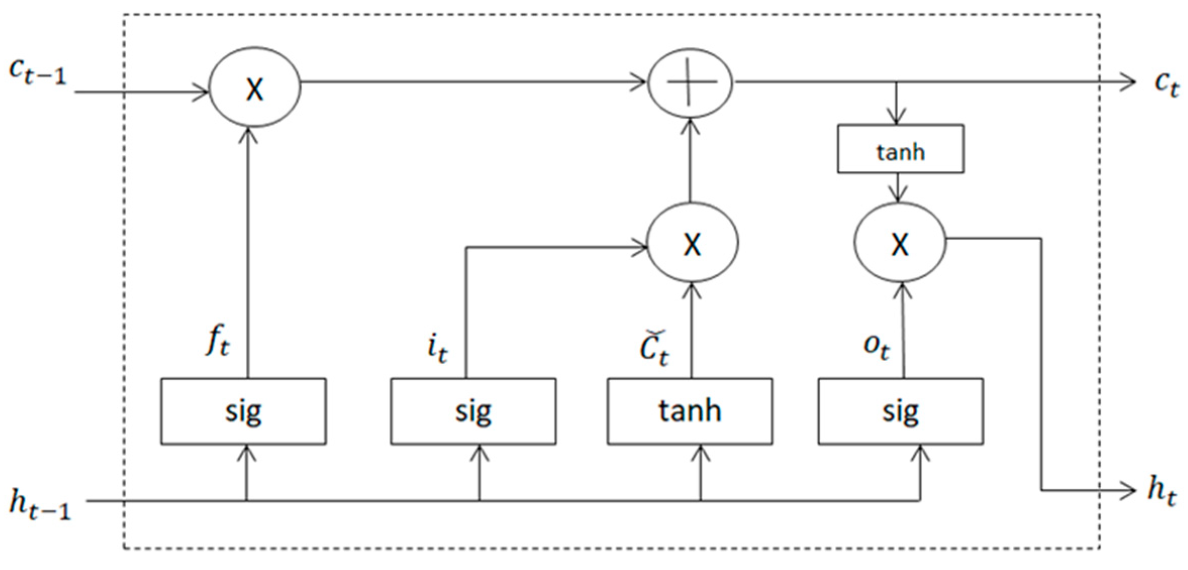
Figure 1. LSTM abstract model.
Sustainability 17 10802 g001
Figure 2. TRP architecture.
Sustainability 17 10802 g002
Figure 3. Hypothesis diagram of TRP model.
Sustainability 17 10802 g003
Figure 4. Workflow of the proposed model architecture.
Sustainability 17 10802 g004
Figure 5. The locations to be visited on the map.
Sustainability 17 10802 g005
Figure 6. The route suggested by the model.
Sustainability 17 10802 g006
Figure 7. Alternative route suggested by user.
Sustainability 17 10802 g007
Figure 8. Comparison of prediction values with actual values.
Sustainability 17 10802 g008
Figure 9. The diagram of average training and validation loss curves for the LSTM.
Sustainability 17 10802 g009
Figure 10. The diagram of average training and validation RMSE curves for the XGBoost.
Sustainability 17 10802 g010
Figure 11. The estimation error distribution of LSTM model.
Sustainability 17 10802 g011
Figure 12. Distribution of features; (a) Distance; (b) Time; (c) Travel mode.
Sustainability 17 10802 g012
Figure 13. Errors demonstration of the models.
Sustainability 17 10802 g013
Figure 14. The bar diagram of error measurements.
Sustainability 17 10802 g014
Figure 15. Comparison of user data and LSTM data on average daily carbon dioxide emissions per person.
Sustainability 17 10802 g015
Figure 16. LSTM-predicted CO2 emissions and distance-oriented user simulation.
Sustainability 17 10802 g016
Figure 17. LSTM-predicted CO2 emissions and comfort-oriented user simulation.
Sustainability 17 10802 g017
Table 1. Sustainability indicators of route optimization and carbon minimization.
CategoryIndicatorsDescription
EnvironmentalCarbon Emissions CO2 emissions per person (Gg CO2)
Energy EfficiencyChange in total CO2 emissions before and after route optimization
EconomicTime EfficiencyChanges in total travel time, transportation options
SocialAccessibilityRoute optimization, time planning
TechnologicalModel PerformanceEvaluation of LSTM and XGBoost models using RMSE, MAE, MSE, and NRMSE metrics
Data IntegrationIncorporation of user interaction and Google API map
Table 2. LSTM training configuration.
Training ComponentConfiguration
Cross-ValidationGroupKFold (N_SPLITS = 5)
Seed EnsembleENSEMBLE_SEEDS = [42, 43, 44, 45, 46]
Batch Size64
Epochs100
EarlyStoppingpatience = 8,
restore_best_weights = True
Learning Rate SchedulingReduceLROnPlateau
(factor = 0.5, patience = 3, min_lr = 1 × 10⁻⁷)
Table 3. XGBoost training configuration.
Training ComponentConfiguration
Max Depth4
Learning Rate0.05
N Estimators (Boosting Rounds)500
Early Stoppingearly_stopping_rounds = 20
L2 Regularization (reg_lambda)1.0
Cross-ValidationGroupKFold (N_SPLITS = 10)
Seed/Random State42
Table 4. LSTM model configuration.
Training ComponentConfiguration
Embeddings(e.g., TravelMode represented with 6 dimensions, with mask_zero = True)
Layer NormalizationApplied after feature fusion
LSTM StackTwo layers
(50 units + 50 units, return_sequences = True)
Dropout0.15
L2 Regularizationλ = 1 × 10⁻⁴
Output LayerTimeDistributed(Dense(1))
Loss FunctionMasked Huber (δ = 0.5)
OptimizerAdam (lr = 2 × 10⁻⁴, clipnorm = 1.0)
Table 5. Route information suggested by the model.
RouteTime (min.)Distance (km)Vehicle
First LocationSecond Location
1 (Housing)2172.6Bus
2340.8Bicycle
3440.6Bicycle
4530.8Bicycle
Table 6. Route information suggested by user.
RouteTime (min.)Distance (km)Vehicle
First LocationSecond Location
1 (Housing)2131.4Bus
23111.2Bus
3470.5Walking
45112.8Bicycling
Table 7. Statistical significance tests results.
ModelWilcoxon Tests Bootstrap Confidence
Interval
Effect Size
Rank-Biserial r_rb
LSTM (RMSE) W = 0.0000,
p = 2.386 × 10⁻¹⁰
Mean difference = 1.6305
95% CI = [1.4843, 1.7873]
−0.8701
LSTM (MAE)W = 0.0000,
p = 2.386 × 10⁻¹⁰
Mean difference = 1.6273
95% CI = [1.5086, 1.7523]
−0.8701
XGBoost (RMSE) W = 0.0000,
p = 1.9531× 10⁻³
Mean difference = 0.101084
95% CI = [0.060589, 0.146333]
−1.0000
XGBoost (MAE)W = 3.0000,
p = 9.766 × 10⁻³
Mean difference = 0.080994
95% CI = [0.040150, 0.119400]
−0.8909
Table 8. Error measurements of the models.
ModelRMSEMAEMSENRMSE
XGBoost0.250.060.062.48
RF1.420.952.0214.21
CatBoost1.270.501.6112.67
LightGBM1.330.891.7713.29
ETR1.320.541.7513.22
MLP0.710.430.507.07
Table 9. Comparative error metrics of deep learning models.
ModelRMSEMAEMSENRMSE
LSTM0.240.060.062.42
RNN0.410.140.174.14
GRU0.310.100.103.13
Table 10. The parameters of fuel consumption.
Fuel TypeIntensity (kg/L)Conversion Factor (TJ/Gg)
(Total CO2)
Carbon Emission Factors (tC/TJ)Oxidation Rate
Diesel0.82043.3320.20.99
Table 11. The molar masses of carbon dioxide and carbon.
SubstanceMolar Mass (g/mol)
Carbon (C)12
Carbon dioxide (CO2)44
Disclaimer/Publisher’s Note: The statements, opinions and data contained in all publications are solely those of the individual author(s) and contributor(s) and not of MDPI and/or the editor(s). MDPI and/or the editor(s) disclaim responsibility for any injury to people or property resulting from any ideas, methods, instructions or products referred to in the content.