When Everyone Loses: Does Air Pollution Create ‘Spurious Equality’?

Abstract

This paper examines how air pollution affects the distribution of labor income within firms. We build a within-firm incentive model and show that air pollution, treated as an exogenous shock, reduces production efficiency and increases operating uncertainty. In response, firms compress both employee and executive compensation. Because executive pay carries a larger weight on performance- and equity-based components and is therefore more sensitive to profit volatility, it declines by more, mechanically narrowing within-firm pay dispersion. At the same time, rank-and-file wages display downward rigidity. The result is a “synchronized decline with sharper cuts at the top,” a form of spurious equality. Using 2014–2022 data on non-financial A-share listed firms in China, we find that a 1% increase in air pollution is associated with a 0.37% average decline in labor income. Effects are stronger in labor-intensive firms and in firms with weaker unions. Two-stage least squares estimates indicate real consequences: talent outflows and reduced innovation. By linking air quality to wage setting, human capital, and innovation, our results reveal a sustainability channel through which pollution undermines decent work and inclusive growth—issues of global relevance for urban economies. The mechanisms we document are likely to generalize beyond China and inform integrated policies that combine environmental regulation with labor-market and innovation policy to support a just and sustainable transition.

1. Introduction

1.1. Background

Since China’s opening-up in 1978, rapid economic growth has been accompanied by pronounced environmental pressures and sizable cross-regional differences in air quality. Air pollution worsens residents’ quality of life, raises infant mortality, and dampens business activity [1]. Despite major efforts by the Chinese government to improve air quality, the Ministry of Ecology and Environment’s Report on National Air Quality in 2023 indicates that more than 40% of cities still fail to meet air quality standards. Moreover, with extreme weather events occurring more frequently, the share of areas facing severe environmental pollution has trended upward in recent years. Over the same period, China’s labor income has risen modestly since 2007 but remains below levels in advanced economies and below the global average [2]. Other studies further indicate that China faces severe income inequality and imbalances in wealth distribution [3]. Our study provides new micro-level evidence on an environmental channel that helps explain China’s slow growth in labor income and persistent distributional inequality.

We focus on a basic question: who bears the cost of air pollution? The adverse health effects of pollution have received wide attention in the literature [4]. Deteriorating air quality leads to numerous health problems, including respiratory infections, cardiovascular disease, and lung cancer [5]. Air pollution is considered a major environmental hazard for human health, affecting not only physical but also psychological, cognitive, and emotional well-being; elevated risks of anxiety, depression, and cognitive decline attest to this [6,7]. Beyond direct health effects, air pollution is linked to a broad range of economic activities [8]. Evidence suggests that higher pollution can worsen mood or heighten risk aversion, distorting subjective probabilities of future events and reducing demand for risky assets [9,10]. Conversely, better weather conditions are associated with more optimistic sentiment and increased financial activity [11,12].

We begin by proposing an optimal compensation-contract model with uncertainty. When air pollution reduces firms’ marginal product and increases earnings volatility, total labor income at the firm level declines. Risk-averse firms tend to lower the intensity of risk-sensitive executive incentives (equity and performance pay) and concomitantly cut executive cash compensation to curb cash outlays [13]. By contrast, nominal wages for rank-and-file employees are constrained by institutional factors such as minimum-wage rules and collective bargaining; firms therefore adjust more on the employment margin—particularly the number of low-skill workers—to compress the overall wage bill [14].

1.2. Research Hypothesis

Air pollution has certain negative externalities, adversely affecting the input of production factors and the quality of the production environment. In areas with more severe air pollution, firms face stricter environmental regulations from local governments. These government regulations compel firms to allocate part of their output to the purchase of green and low-carbon equipment or to adopt stricter emission reduction measures [15]. Consequently, companies must invest more in green capital to combat pollution, which undoubtedly increases their operational costs. To ensure maximization of profits, firms may reduce the scale of employment in the short term to cope with rising production costs. The crowding-out effect of production factors leads to a decline in labor share within firms.

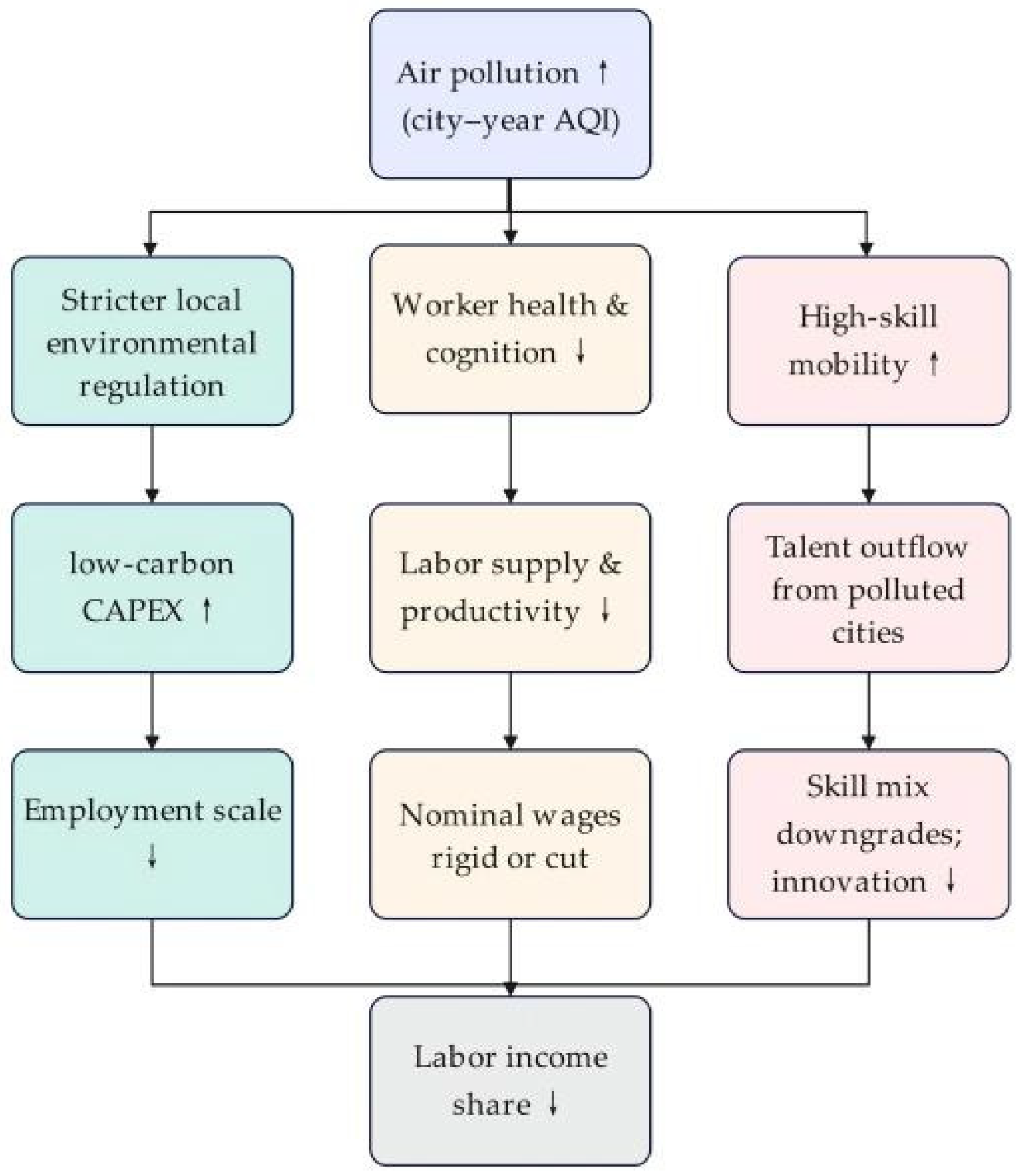
Moreover, air pollution also impacts employees’ productive activities. On one hand, air pollution can severely damage employees’ cognitive abilities and physical health. Employees may choose to reduce their labor supply and lower their productivity during periods of high air pollution, especially in outdoor occupations. Additionally, employees who commute long distances might opt for remote work or take leave to avoid the hazards of air pollution during their commute, which would also decrease the labor supply and reduce employee income. On the other hand, in China, employees are typically at a disadvantage in wage negotiations [16], leading companies facing continually declining labor productivity to often reduce wages to decrease costs. This undeniably has a negative impact on the labor share (Figure 1).

Incontestably, air pollution is becoming an increasingly critical factor influencing the occupational decisions of the labor force [17]. Prolonged exposure to significant air pollution levels elevates the risk of developing respiratory ailments and lung cancer among workers. Meanwhile, air pollution also profoundly affects employees’ families, particularly impacting the elderly and children more adversely than adults [18].

As the market economy rapidly develops and barriers to labor mobility decrease, employees are increasingly moving to areas with lower air pollution to reduce its risks. Employees with higher education and technical skills, who face lower mobility costs and have greater advantages in the job market, are more likely to relocate to cities with better air quality in response to pollution’s adverse effects [19]. These employees are more concerned about how air pollution impacts their health, which gives them greater mobility. As a result, air pollution’s brain drain effect is stronger in companies with higher levels of human capital [20,21]. The loss of high-skilled talent, which is crucial for a company’s human capital, leads to a reduction in labor income share. A formal analysis of the underlying mechanism is provided in the Supplementary Materials.

1.3. Main Findings and Contributions

We measure air quality by the average concentrations of six pollutants, including common measures such as PM_2.5 and CO. Air-pollution data come from ground monitoring stations that have been built out since 2012 to cover China’s major prefecture-level cities. We aggregate daily city-station readings into annual averages to construct a city–year measure of pollution intensity. Listed firms are mapped to cities based on their registered location or principal place of business, and firm-year financials are obtained from annual reports. We define a firm’s labor income share as the ratio of employee compensation to output. To account for unobserved factors affecting labor income, our baseline identification includes industry and year fixed effects. Using the Air Quality Index (AQI) available since 2013, we find that firms located in regions with worse air quality exhibit significantly lower labor income within the firm. Quantitatively, a 1% increase in air pollution is associated with a 0.37% decline in firm-level labor income.

We evaluate several threats to identification. First, our AQI measure may not fully capture true pollution. Replacing AQI with annual averages of single pollutants (PM₂.₅, PM₁₀, SO₂, NO₂, CO, O₃) leaves the core results unchanged. Among these, O₃ shows the largest negative effect on labor income, followed by PM₁₀. Second, results may be sensitive to the sample period. Splitting the sample at 2017 yields no meaningful change in significance, and controlling for time trends produces consistent conclusions. Third, findings could be driven by specific cities. Excluding highly polluted regions and the large metropolitan areas of Beijing, Shanghai, Guangzhou, and Shenzhen does not alter the results. Fourth, estimation concerns remain. We introduce stricter city fixed effects and adjust clustering to the industry-year and city-year levels to account for error correlation. Fifth, measurement of labor income may not perfectly reflect employees’ actual earnings. In Section 3.2.4., we redefine firm labor income and standardize it by industry-year means; the overall evidence confirms the robustness of our baseline identification.

Causal identification may still face reverse-causality and omitted-variable concerns. First, firms’ compensation structures and profit-sharing schemes could shape environmental investment and emissions, thereby feeding back into local pollution levels. Second, regional differences in economic structure or policy could jointly affect pollution and labor income, introducing omitted-variable bias. To mitigate endogeneity, we use thermal inversion days as an instrumental variable. Typically, atmospheric temperature decreases with altitude, and the resulting convection disperses pollutants, lowering pollution levels. During thermal inversions, however, temperature rises with altitude, suppressing convection and trapping pollutants, thereby intensifying pollution. Inversion strength is, in theory, determined by complex meteorological systems and is exogenous to firm-level outcomes. Hence, using inversion strength as an instrument satisfies both relevance and exogeneity. Two-stage least squares (2SLS) estimates indicate that a 1% increase in air pollution reduces firm labor income by 0.74%, roughly twice the OLS estimate.

We use “spurious equality” to denote a decline in within-firm pay dispersion that is driven by disproportionate cuts at the top under pollution-induced uncertainty, while rank-and-file wages remain bound by downward nominal rigidity. This compression does not reflect welfare gains for lower-paid workers and is typically accompanied by employment adjustments and weaker innovation. This differs from “transitory equality,” a short-lived, symmetric and reversible compression that fades as temporary shocks dissipate, and from “artificial reduction of inequality,” a compression created by accounting or policy devices rather than real risk and cash-flow constraints. The stability of labor income is a key concern for policymakers, as it reflects distributive fairness and strongly influences long-term social stability and sustainable growth. Since disposable household income is primarily composed of labor income, a declining labor share threatens social equity, justice, and political stability [22]. We document the economic consequences of reduced firm labor income. Treating pollution-induced changes in labor income as an exogenous driver, we find that firms’ human-capital structures and innovative activity deteriorate significantly: the share of highly educated employees (bachelor’s degree or above) declines, the share of low-skill workers (below high school) rises, and both total patents and invention patents fall.

We further examine within-firm labor income distribution and show that air pollution compresses internal pay gaps through “larger cuts at the top”. Executive cash and equity compensation both decline significantly, while employees’ nominal pay is broadly insensitive. After standardizing compensation within industries, pollution significantly lowers the executive pay premium but does not affect the employee pay premium, resulting in a narrower premium gap. Moreover, in firms with higher stock-price volatility, the suppressing effect of pollution on equity-based pay is stronger; the negative impact on executive cash pay is somewhat attenuated but remains negative overall, consistent with the basic rigidity of nominal employee wages.

Our contributions are threefold. First, we add to research on how air pollution affects firms’ human capital. Prior work shows that improved air quality stabilizes labor supply and raises productivity [23,24,25,26,27], while pollution increases absenteeism and sick leave and reduces the efficiency of human-capital utilization [28,29]. Direct evidence on how pollution shapes human capital within firms remains scarce. By analyzing a factor that has received limited attention—air pollution’s impact on firm-level labor income shares—we extend the discussion of the declining labor share. Second, we broaden the study of the economic consequences of a falling labor share. Our empirical results document a talent-loss effect—pollution leads to outflows of high-skill labor—and we show a further consequence: reduced innovation output. Third, we contribute to the literature on income distribution between executives and employees.

Our findings speak directly to the sustainability agenda by identifying a firm-level channel through which degraded air quality undermines decent work (via pay compression and wage rigidity), inclusive growth (through a falling labor share and widening distributional risks), and innovative capacity (via talent outflows and reduced high-quality patents). These mechanisms are not specific to China’s institutional setting: urbanization, transboundary pollution, and exposure to episodic shocks (e.g., thermal inversions, wildfires, dust storms) are common across both advanced and emerging economies. The link we document between environmental quality, wage-setting under risk, and human-capital allocation thus has broad applicability and policy salience. It also complements climate and air-pollution co-benefit strategies by showing that cleaner air can help preserve the labor share and sustain innovation during green transitions. Taken together, the results provide micro-level evidence to inform integrated policies that combine environmental regulation with labor-market and innovation policies in support of a just and sustainable transition worldwide.

The remainder of the paper is organized as follows. Section 2 (“Material and Method”) describes data sources, variable construction, and our hypotheses. Section 3 provides empirical evidence on the effects of air pollution on firm-level labor income shares, including baseline results, robustness checks, endogeneity analyses, and cross-sectional heterogeneity. Section 4 delves into within-firm labor income distribution. Section 5 concludes.

2. Material and Method

2.1. Main Variables

2.1.1. Air Pollution

We sourced daily Air Quality Index (AQI) data for Chinese cities from the China Ministry of Environmental Protection’s official website to assess our paper’s key explanatory variable—air pollution. Air pollution levels are evaluated using the natural logarithm of the average daily AQI for each year and city. In our empirical evaluation, we primarily employ the Air Quality Index (AQI) as the fundamental explanatory variable [30,31,32].

2.1.2. Labor Income Share

Based on prior research, we extracted labor income share data from the financial statements of listed companies [33]. We define labor income share (LnLS) as the payment to employees divided by the firm’s value-added and log-transform this ratio for analysis. Here, employee compensation is represented by the accounting line item “payroll payable”, while the firm’s value added is calculated as operating revenue minus operating costs plus employee compensation payments plus depreciation of fixed assets. Furthermore, this paper uses “cash paid to employees” from the balance sheet as an alternative variable for employee compensation to test the stability of our results under different definitions.

2.2. Control Variables

To address confounding factors and ensure valid inference, we include the following controls [34,35]: (1) Asset size (Size), the logarithm of total assets; (2) Operating cash flow (Cash), cash flow from operations divided by total assets; (3) Sales revenue (Sales), the change in sales divided by total assets; (4) Leverage (Lev), total liabilities divided by total assets; (5) Tobin’s q (Tobinq), (market value of equity + total debt)/total assets (market value of equity + total debt)/total assets; (6) Top ten shareholding (Top10), the percentage of shares held by the top ten shareholders; (7) Independent directors (Ind), independent directors divided by total board members; and (8) CEO duality (Dual), equal to 1 if the chairman and general manager are the same person, and 0 otherwise.

2.3. Data Sources

We use data from 2014 to 2022 on companies listed on China’s Shanghai and Shenzhen A-shares, sourced from the CSMAR (China Stock Market & Accounting Research, Shenzhen, China) database. Air pollution data are obtained from the daily Air Quality Index provided by China’s National Environmental Monitoring Center. In processing the data, the following steps were taken: First, companies listed as ST or *ST are excluded to prevent the potential unreliability of accounting information from companies in financial distress. Second, due to significant differences in business models and financial statements between financial and non-financial firms, listed companies in the finance and insurance sectors are further removed. Third, to avoid the interference of outliers, all continuous variables are winsorized at the 1% and 99% quantiles. Lastly, observations with missing values for main variables are omitted. This results in a total of 20,619 company-year observations.

Table 1. Summary statistics for main variables.

Variables	Obs.	Mean	S.D.	Min	P25	P50	P75	Max
LnLS	20,619	−2.1488	1.0801	−11.7550	−2.6339	−2.0109	−1.4623	−0.0031
AQI	20,619	4.3077	0.2618	3.4326	4.1139	4.3138	4.4793	5.1668
Size	20,619	22.4070	1.2974	18.9750	21.4720	22.2110	23.1670	26.1020
Cfo	20,619	0.0553	0.0656	−0.1909	0.0178	0.0533	0.0920	0.2578
Sales	20,619	0.0680	0.1461	−0.5237	0.0003	0.0511	0.1217	0.7153
Leverage	20,619	0.4120	0.1939	0.0530	0.2574	0.4051	0.5526	1.0539
Tobinq	20,619	2.0829	1.3188	0.8559	1.2481	1.6609	2.4049	8.1714
Top10	20,619	0.5891	0.1478	0.2278	0.4835	0.5956	0.6989	0.9492
Ind	20,619	0.3768	0.0535	0.1429	0.3333	0.3636	0.4286	0.5714
Dual	20,619	0.2949	0.4560	0	0	0	1	1

reports the variable definitions for the baseline strategy. Data cleaning and analyses were conducted in Stata 16, and selected figures were produced in Python 3.11.

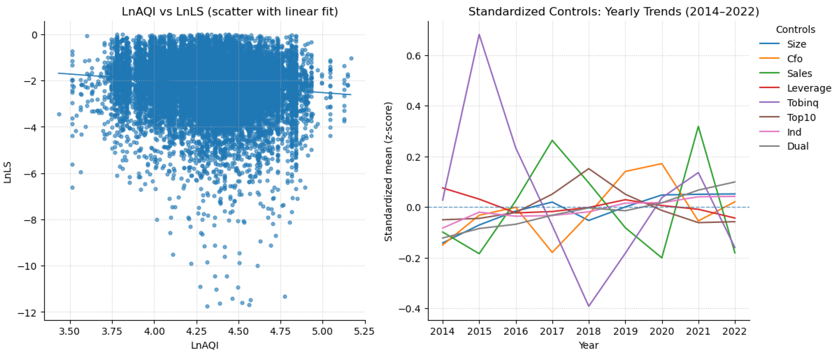
Table 1 reports the descriptive statistics results for the main variables used in this paper. The mean value of LnLS is −2.1488 with a standard deviation of 1.0801, indicating significant differences in labor income share among enterprises. The average value of air pollution is 4.3077 with a standard deviation of 0.2618, suggesting that the air pollution level in most cities in China is at an average level (Figure 2).

2.4. Empirical Model

To identify air pollution’s effect on labor income share, the basic empirical model is as follows:

$$LnL{S}_{it}={\alpha }_0+{\alpha }_{1}AQ{I}_{jt}+{\alpha }_{2}Controls+{\mu }_k+{\gamma }_t+{\epsilon }_{it}$$

(1)

where i represents the firm, and t represents the year; LnLS denotes the firm’s labor income share; AQI represents the average air pollution quality index for the city where the enterprise is located; Controls denotes a collection of control variables, while ε symbolizes the random error term, which is presumed to follow an independent and identical distribution. Additionally, we adjust for both industry and year fixed effects to address unobserved characteristics that vary over time at the industry level. The coefficient α₂ is of particular interest, as it quantifies the effect of urban air pollution on labor income.

3. Results and Discussions

3.1. Benchmark Model Results

Baseline regression results.

Table 2. The benchmark model results.

	(1)	(2)	(3)
Variables	LnLS	LnLS	LnLS
AQI	−0.5339 ***	−0.3770 ***	−0.3746 ***
	(0.0577)	(0.0618)	(0.0613)
Size			−0.1289 ***
			(0.0174)
Cfo			−1.6757 ***
			(0.1585)
Sales			−0.5419 ***
			(0.0631)
Leverage			0.9163 ***
			(0.0963)
Tobinq			−0.0361 **
			(0.0153)
Top10			−0.2434 **
			(0.0991)
Ind			−0.0353
			(0.2329)
Dual			−0.0459
			(0.0284)
Constant	0.1509	−0.5249 **	2.3516 ***
	(0.2457)	(0.2648)	(0.4766)
Year FE		√	√
Industry FE		√	√
Obs.	20,618	20,617	20,617
Adj-R2	0.0167	0.1533	0.1988

Note: *** and ** denote statistical significance at the 10% and 5% levels, respectively, with robust standard errors clustered at the firm level in parentheses. A check mark (√) indicates that the specification includes the corresponding fixed effects or control variables. The same notation applies to the following tables.

reports the baseline estimates from Equation (1). In column (1), we do not include any control variables. The coefficient on AQI is negative and statistically significant: a 1% increase in city-level air pollution is associated with a 0.53% decline in the share of labor income in firm revenue. This is a sizable effect, indicating that worsening air quality substantially depresses labor income within firms.

In column (2), after adding the pre-selected controls, the AQI coefficient remains significantly negative, though its magnitude is smaller than in column (1). In column (3), we adopt the full specification with year and industry fixed effects to mitigate biases from unobserved industry factors and time trends. The estimated AQI coefficient stabilizes at a smaller magnitude: a 1% rise in air pollution is associated with a 0.37% reduction in labor income, equivalent to 17% of the sample mean (0.3746/2.1488).

Taken together, columns (1)–(3) in Table 2 support our hypothesis that increases in air pollution reduce labor income within firms.

3.2. Robustness Check

3.2.1. Alternative Measures of Air Pollution

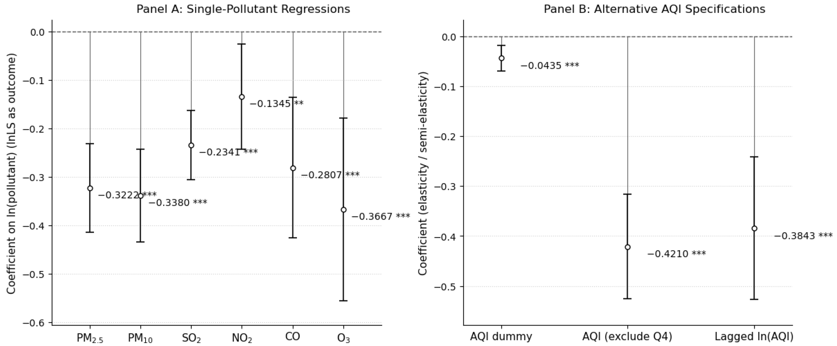
China’s Air Quality Index (AQI), released by the National Environmental Monitoring Center, is a composite of six pollutants (SO₂, NO₂, PM₂.₅, PM₁₀, CO, and O₃). Because pollutant weights and regional heterogeneity may cause a single index to imperfectly capture economic impacts, we re-estimate Equation (1) using the annual mean concentration of each pollutant separately. Figure 3, Panel A plots the point estimates and 95% confidence intervals from these single-pollutant regressions (outcome: lnLS). Relative to CO and SO₂, particulate matter (PM₂.₅/PM₁₀) and O₃ show larger negative effects on labor income.

Next, we define AQI_dummy (1 for cities with AQI above the sample mean; 0 otherwise) and re-estimate Equation (1) with this indicator. Figure 3, Panel B shows that firms in higher-pollution areas have labor income that is about 4% lower than in lower-pollution areas. Panel B also reports two robustness checks: excluding Q4 observations when computing city-level AQI and using lagged ln(AQI); both yield significantly negative coefficients in line with the baseline.

Finally, because local environmental assessment and performance systems could influence reported pollution—raising concerns about “monitoring intervention” or “data smoothing”—we re-compute AQI excluding fourth-quarter readings and also use lagged AQI. We find no evidence of assessment-driven misreporting, and the lagged specification corroborates our main results. Overall, the AQI measure we employ appears to capture city-level air quality well for our purposes.

3.2.2. Subsample Analysis

During our sample period, China underwent several rounds of environmental governance and macro shocks, including the “Blue Sky Protection Campaign” launched in 2017 and the COVID-19 lockdowns in 2020. If nationwide policies or sudden events caused sharp, year-specific swings in air quality, the estimated changes in labor income might capture time trends rather than true firm-level responses. To address this concern, we split the sample into two subperiods—2014–2017 and 2018–2022—and estimate the model separately. As shown in columns (1)–(2) of

Table 3. Subsample analysis.

Variables	(1)	(2)	(3)	(4)
	LnLS	LnLS	LnLS	LnLS
AQI	−0.4980 ***	−0.2904 ***	−0.3699 ***	−0.1998 ***
	(0.0833)	(0.0609)	(0.0676)	(0.0750)
Constant	1.5727 **	2.4337 ***	2.4558 ***	2.2154 ***
	(0.7635)	(0.4400)	(0.5486)	(0.6414)
Controls	√	√	√	√
Year FE	√	√	√	√
Industry FE	√	√	√	√
Obs.	6953	13,664	17,923	14,367
Adj-R2	0.1670	0.2161	0.1986	0.2004

Note: *** and ** denote statistical significance at the 10% and 5% levels, respectively, with robust standard errors clustered at the firm level in parentheses. A check mark (√) indicates that the specification includes the corresponding fixed effects or control variables.

, the pollution coefficients have the same sign and are statistically significant in both subperiods, indicating that our findings are not driven by short-term events.

Air pollution in China is geographically concentrated, especially in the Beijing–Tianjin–Hebei region and the Yangtze River Delta. If changes in pollution and in firms’ distributional outcomes were concentrated in a few heavily polluted areas, our estimates might simply be pulled by those locales rather than reflect a general pattern. To test this possibility, we sequentially exclude (i) cities in the heavily polluted Beijing–Tianjin–Hebei region and (ii) the four megacities—Beijing, Shanghai, Guangzhou, and Shenzhen—and re-estimate the model. As reported in columns (3)–(4), the estimated AQI coefficient remains statistically significant and negative in these subsamples, confirming that our conclusions are not driven by particular cities.

3.2.3. Alternative Measures of Identification Specification

Our baseline specification includes the main firm-level controls and incorporates both industry and year fixed effects to absorb industry heterogeneity and macro shocks. While this setup helps identify the net effect of air pollution on within-firm income distribution, two concerns remain. First, regional policies or environmental shocks may impose common influences on firms within the same city. Second, error terms may exhibit temporal or spatial correlation, potentially affecting standard errors and inference.

We adopt five approaches to address these identification concerns. First, we add city fixed effects to soak up unobserved, time-invariant city-level factors. Second, we account for time trends and their interaction with control variables and province fixed effects. Finally, we allow for serial correlation by employing two-way clustering of standard errors at the city–year and industry–year levels.

Table 4. Alternative measures of identification specification.

	(1)	(2)	(3)	(4)	(5)
Variables	LnLS	LnLS	LnLS	LnLS	LnLS
AQI	−0.2701 ***	−0.3677 ***	−0.3773 ***	−0.3746 ***	−0.3746 ***
	(0.0819)	(0.0734)	(0.0612)	(0.0472)	(0.0328)
Constant	1.9038 ***	2.3266 ***	2.2402 ***	2.3516 ***	2.3516 ***
	(0.4956)	(0.5292)	(0.4998)	(0.2233)	(0.2836)
Control	√	√	√	√	√
Control × Trend			√
City FE	√
Province × Trend		√
Year FE	√	√	√	√	√
Industry FE	√	√	√	√	√
Obs.	20,605	20,617	20,617	20,617	20,617
Adj-R2	0.2517	0.2137	0.2014	0.1988	0.1988
Cluster	Firm	Firm	Firm	City Year	Industry Year

Note: *** denote statistical significance at the 10% levels, respectively, with robust standard errors clustered at the firm level in parentheses. A check mark (√) indicates that the specification includes the corresponding fixed effects or control variables.

, columns (1)–(5), report the results; we find no evidence that our conclusions are driven by biases arising from the identification strategy.

3.2.4. Alternative Measures of Labor Income Share

In this section, we construct alternative indicators for labor share from different perspectives. Labor share can be defined as the proportion of labor income to the value added by the enterprise. Companies typically disclose the cash paid to employees in the cash flow statement. Therefore, we use this as an alternative measure for corporate labor compensation, calculating labor income share as cash paid to employees divided by (total operating revenue—total operating cost + cash paid to employees + depreciation of fixed assets), and log-transform this ratio (LnLS1). Additionally, net profit represents a company’s actual value added, so we use the ratio of cash paid to employees to net profit as another measure for labor share and log-transform it (LnLS2). To account for industry variations, we also adjust for labor share by using industry averages (Adj_mean_LnLS). After substituting labor income share with these alternative measures, our results remain unchanged (

Table 5. Alternative measures of labor income share.

	(1)	(2)	(3)
Variables	LnLS1	LnLS2	Adj_mean_LnLS
AQI	−0.1011 ***	−0.1371 ***	−0.3604 ***
	(0.0231)	(0.0515)	(0.0609)
Constant	1.9268 ***	6.3672 ***	4.3149 ***
	(0.1747)	(0.3704)	(0.4745)
Controls	√	√	√
Year FE	√	√	√
Industry FE	√	√	√
Obs.	20,614	19,658	20,617
Adj-R2	0.3518	0.3002	0.0532

Note: *** denote statistical significance at the 10% levels, respectively, with robust standard errors clustered at the firm level in parentheses. A check mark (√) indicates that the specification includes the corresponding fixed effects or control variables.

).

3.3. Endogeneity Concerns

3.3.1. Instrumental-Variable Estimation

We use the number of thermal inversion days in a firm’s city (Thermal_Inversion) as an instrument for air pollution in a two-stage least squares (2SLS) model [1].

Table 6. Instrumental Variable.

	(1)	(2)	(3)	(4)
Variables	AQI	LnLS	AQI	LnLS
VC	0.0021 ***		0.0021 ***
	(0.0000)		(0.0000)
AQI		−0.7267 ***		−0.7467 ***
		(0.1119)		(0.1137)
Controls		√		√
YEAR FE	√	√	√	√
Firm FE	√	√	√	√
Obs.	20,614	20,614	20,614	20,614
K-P rk Wald F statistic	920.01		2657.58
K-P rk LM statistic	2725.24		907.64

Note: *** denote statistical significance at the 10% levels, respectively, with robust standard errors clustered at the firm level in parentheses. A check mark (√) indicates that the specification includes the corresponding fixed effects or control variables.

presents the instrumental-variable (IV) results. Columns (1) and (3) show the first-stage regressions, with the coefficient on Thermal_Inversion being positive and significant at the 1% level. Columns (2) and (4) present the second-stage estimates: the coefficient on AQI is −0.7467, about twice the baseline magnitude, and remains significant at the 1% level. These results support the view that air pollution significantly reduces within-firm labor income. Instrument strength and validity diagnostics indicate that the instrument is reliable, with Wald F-statistics and LM statistics of 77.560 and 77.290, both exceeding conventional thresholds for weak instruments and overidentification tests. The IV magnitude exceeding OLS is consistent with attenuation from pollution mismeasurement and with a LATE concentrated among inversion-exposed firms; the strong first stage reduces concerns about weak instruments.

3.3.2. Placebo Test

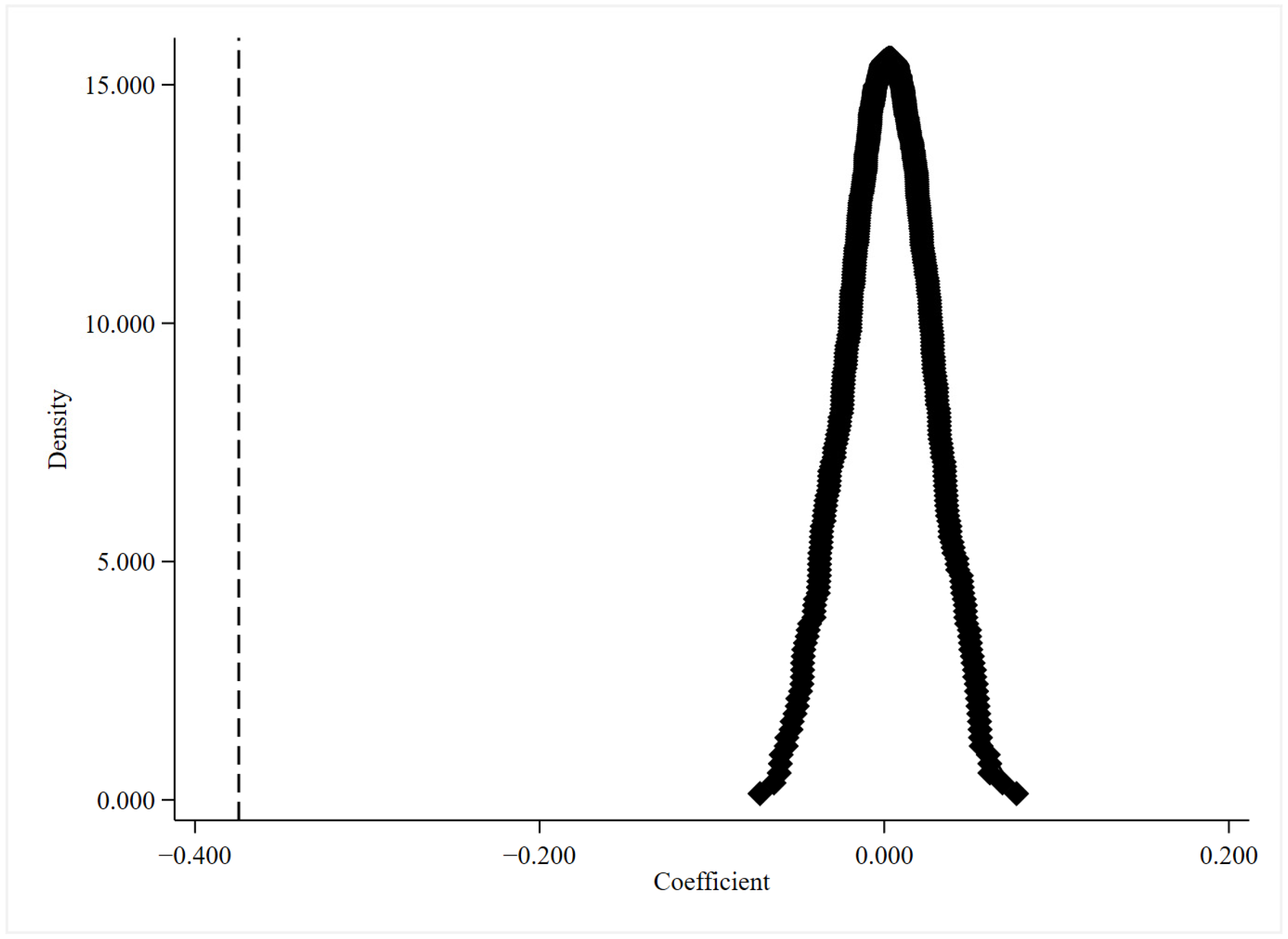
In this section, we implement a placebo test to further enhance the credibility of our results. Specifically, we randomly assign a fictitious AQI value to each city for each year, log-transform these values, and then use them to replace our explanatory variable of air pollution to re-estimate Equation (1). We repeat this regression 500 times and display the probability density of the fictitious AQI (FAQI) coefficients in Figure 1, where the dashed line represents the actual regression coefficient estimate. Figure 1 indicates that our real coefficient estimate deviates from the placebo coefficient estimates, suggesting that our estimation results are largely not driven by omitted variables or measurement errors (Figure 4).

3.4. Heterogeneity Analysis

Unions play a non-negligible role in determining the distribution of labor income. We examine how unionization moderates the decline in labor income induced by air pollution. Following prior work, we define Union as the natural logarithm of a firm’s union expenditures in the current year. Column (1) of

Table 7. Heterogeneity analysis.

	(1)	(2)
Variables	LnLS	LnLS
AQI	−2.5298 ***	−2.1615 ***
	(0.3058)	(0.5756)
Union	−0.4877 ***
	(0.0844)
Capital_intensity		−0.3966 ***
		(0.1228)
Union × AQI	0.1380 ***
	(0.0200)
Capital_intensity × AQI		0.0874 ***
		(0.0283)
Constant	12.5190 ***	10.0375 ***
	(1.4148)	(2.4952)
Controls	√	√
YEAR FE	√	√
Firm FE	√	√
Obs.	17,726	20,617
Adj-R2	0.2634	0.2005

Note: *** denote statistical significance at the 10% levels, respectively, with robust standard errors clustered at the firm level in parentheses. A check mark (√) indicates that the specification includes the corresponding fixed effects or control variables.

shows that firms with stronger union power experience smaller reductions in labor income when air quality deteriorates. This result is consistent with nominal wage rigidity: by strengthening floors on wages and benefits, unions weaken the transmission of pollution shocks to labor compensation, thereby limiting the decline in labor income.

The mix of capital and labor inputs shapes how firms adjust to pollution shocks. Capital-intensive firms can more readily spread shocks by varying capital utilization and project timing, whereas labor-intensive firms rely more on rapid headcount adjustments, making them more susceptible to declines in the labor share. We therefore hypothesize that the effect of air pollution on labor income is weaker in capital-intensive firms. We measure capital intensity (CapInt) as the ratio of net fixed assets to the number of employees.

Column (2) of Table 7 indicates that the negative effect of air pollution on the labor income share is significantly attenuated in firms with higher capital intensity. In other words, when pollution worsens, labor-intensive firms are more inclined to reduce employment rather than cut average wages, which lowers the total wage bill and, in turn, reduces the labor share.

4. Further Analysis

4.1. Consequences of Declining Labor Income

In this section, we examine the consequences of a decline in the labor income share. To ensure causal identification, we employ two-stage least squares (2SLS), treating the labor income share as an endogenous regressor and using the number of thermal inversion days as an instrument to isolate its exogenous component. Our outcome variables include the shares of employees with (i) a bachelor’s degree or above, (ii) a graduate degree or above, and (iii) a high-school education or below, as well as the logarithms of (iv) total patent applications and (v) invention patent applications.

As reported in

Table 8. Consequences of declining labor income.

	(1)	(2)	(3)	(4)	(5)
Variables	ex_pay	em_pay	paygap	ex_premium	em_premium
LnLS	−0.1467 ***	−0.0638 ***	0.2391 ***	0.3270 *	0.3348 **
	(0.0312)	(0.0143)	(0.0736)	(0.1686)	(0.1663)
Controls	√	√	√	√	√
Year FE	√	√	√	√	√
Industry FE	√	√	√	√	√
Obs.	19,392	16,150	11,463	20,614	20,614
K-P rk Wald F statistic	42.95	38.99	18.43	44.51	44.51
K-P rk LM statistic	40.67	36.72	17.92	42.11	42.11

Note: ***, **, and * denote statistical significance at the 10%, 5%, and 1% levels, respectively, with robust standard errors clustered at the firm level in parentheses. A check mark (√) indicates that the specification includes the corresponding fixed effects or control variables.

, columns (1)–(5), the pollution-induced reduction in the labor income share has meaningful effects on firms’ human-capital structure and innovation activity. Specifically, the proportion of employees with a bachelor’s degree or higher—and especially those with graduate degrees—declines, while the share of workers with a high-school education or below rises. This pattern indicates a skill downgrading and quantity expansion at the lower end of the workforce as firms adjust under distributive contraction. At the same time, both total patent applications and invention patents fall significantly, with a stronger suppression of invention patents, suggesting that high-quality innovation is more adversely affected when the labor share contracts. These findings align with our core mechanism: when the labor share is compressed, firms prioritize maintaining basic operations over engaging in riskier, longer-horizon innovation.

Overall, the pollution-induced decline in the labor income share does not simply reduce costs; it constitutes a “distributive contraction” marked by a lower share of high-skill talent and weakened high-quality innovation—further corroborating the paper’s notion of “spurious equality.”

4.2. Distribution of Labor Income

To assess how air pollution affects the distribution of labor income within firms, we constructed six alternative indicators based on previous research methodologies [36]. (i) Executive pay (ex_pay): the ratio of total compensation to the number of executives, excluding independent directors and unpaid executives. (ii) Employee pay (em_pay): total compensation for non-executive employees divided by the number of rank-and-file employees (executive pay excluded). (iii) Internal pay gap (pay_gap): the ratio ex_pay/em_pay. (iv) Executive pay premium: ex_pay relative to the industry–year median, capturing a firm’s executive pay benchmarked to its industry peers. (v) Employee pay premium: em_pay relative to the industry–year median, comparing average employee pay across firms within the same industry. (vi) Pay-gap premium: the ratio of the executive pay premium to the employee pay premium, measuring how a firm’s internal pay gap deviates from its industry counterpart.

Columns (1)–(6) of

Table 9. Distribution of labor income.

	(1)	(2)	(3)	(4)	(5)	(6)
Variables	ex_pay	em_pay	paygap	ex_premium	em_premium	gap_premium
AQI	−0.3162 ***	0.0099	−2.3186 ***	−0.5311 ***	0.0425	−0.6617 ***
	(0.0370)	(0.0070)	(0.2513)	(0.0619)	(0.0319)	(0.0737)
Constant	−4.9757 ***	−0.3928 ***	−20.3141 ***	−8.1489 ***	−1.9857 ***	−5.6936 ***
	(0.3229)	(0.0560)	(1.9352)	(0.5246)	(0.2742)	(0.5448)
Controls	√	√	√	√	√	√
Year FE	√	√	√	√	√	√
Firm FE	√	√	√	√	√	√
Obs.	20,610	20,614	20,607	20,575	20,614	20,572
Adj-R2	0.3167	0.0858	0.2507	0.2689	0.0393	0.1831

Note: *** denote statistical significance at the 10% levels, respectively, with robust standard errors clustered at the firm level in parentheses. A check mark (√) indicates that the specification includes the corresponding fixed effects or control variables.

show that air pollution exerts a consistent directional impact on within-firm income distribution. In terms of levels, air pollution significantly depresses executive average pay, while its effect on employee average pay is statistically insignificant. This asymmetric response—“down at the top, unchanged at the bottom”—is consistent with nominal wage rigidities arising from minimum-wage rules and collective bargaining. Regarding within-firm dispersion, because executive pay declines more while employee pay is stickier, the internal pay gap (pay_gap) narrows significantly. Crucially, this narrowing does not reflect an improvement at the bottom; rather, it is driven by a larger compression at the top—what we term “spurious equality.”

Finally, after industry standardization, air pollution significantly lowers the executive pay premium but leaves the employee pay premium insignificant, thereby reducing the pay-gap premium. This indicates that, under pollution shocks, firms cut executive pay faster relative to industry peers, rather than the result being a uniform, industry-wide decline.

4.3. Executive Equity Pay and Firm Risk

Executive compensation is not limited to cash; a substantial component consists of equity-based incentives tied to performance and risk, which better reflect a firm’s incentive design for value creation. Following related studies, we measure executive equity pay (Ex_Stkcd) as the fair value of equity-based compensation granted at the firm level in the current year. Firm risk (CRT) is measured by the standard deviation of the firm’s stock returns within the year; higher CRT indicates greater stock-price volatility and higher uncertainty.

Table 10. Executive equity pay and firm risk.

	(1)	(2)	(3)	(4)
Variables	ex_stkcd	ex_stkcd	ex_pay	em_pay
CRT		3.4058 **	−0.1162 *	−0.0169 *
		(1.4067)	(0.0691)	(0.0098)
AQI	−1.4806 ***	0.6674	−0.3980 ***	−0.0012
	(0.3244)	(0.9431)	(0.0692)	(0.0107)
CRT × AQI		−0.7222 **	0.0268 *	0.0037 *
		(0.3025)	(0.0155)	(0.0022)
Constant	4.2984 *	−6.7523	−4.6252 ***	−0.3391 ***
	(2.2808)	(4.9082)	(0.3740)	(0.0681)
Controls	√	√	√	√
Year FE	√	√	√	√
Firm FE	√	√	√	√
Obs.	16,172	16,172	20,610	20,614
Adj-R2	0.1538	0.1558	0.3173	0.0858

Note: ***, **, and * denote statistical significance at the 10%, 5%, and 1% levels, respectively, with robust standard errors clustered at the firm level in parentheses. A check mark (√) indicates that the specification includes the corresponding fixed effects or control variables.

, columns (1)–(4), reports the key results on executive equity pay and risk. First, columns (1)–(2) show that the coefficient on AQI for Ex_Stkcd is significantly negative, indicating that higher air pollution reduces executive equity compensation on average. When we include the interaction CRT × AQI, the interaction term is significantly negative, implying that in riskier firms the suppressing effect of pollution on equity-based incentives is stronger. In other words, pollution-induced uncertainty and cash-flow pressure lead firms—especially when risk is high—to scale back equity compensation that is tightly linked to performance, thereby lowering contractual exposure to risk.

Second, column (3) shows that air pollution also depresses executive cash pay. The coefficient on CRT × AQI is positive and significant, suggesting that in high-risk states the negative impact of pollution on executive cash compensation is somewhat attenuated—though not enough in our sample to overturn the overall negative effect. Column (4) contrasts with these patterns by showing that employee nominal wages are rigid: air pollution does not significantly reduce rank-and-file pay.

5. Conclusions and Policy Recommendations

5.1. Conclusions

When everyone bears the costs of air pollution, who pays more? This paper examines how pollution affects the level and distribution of labor income. Combining prefecture-level daily air-quality data from the Ministry of Ecology and Environment with a panel of non-financial A-share listed firms, we document a causal relationship between local air pollution and firms’ labor income shares. The effect is stronger among private and labor-intensive firms and in firms with weaker union resources. We further show that firms with a larger stock of high-skill employees are more exposed to pollution shocks; a talent-outflow channel contributes to the decline in the labor share. Finally, focusing on this channel, pollution reduces the employee component of the labor share with limited impact on the executive component, consistent with our broader evidence of top-end pay compression alongside nominal wage rigidity. Overall, pollution significantly depresses the labor share and, via talent loss, generates a “distributive contraction” that underpins the paper’s notion of “spurious equality.”

Our findings complement evidence that air-quality improvements stabilize labor supply and productivity and are consistent with studies linking pollution to employee treatment and executive pay [23]. Relative to this literature, we highlight a within-firm distribution channel—through the labor income share and pay compression—that helps explain talent outflows and weakened innovation [30]. Recent evidence on airborne micro- and nanoplastics highlights additional pathways through which air quality may affect human health and productivity, thereby reinforcing the sustainability relevance of our results [37].

5.2. Policy Recommendations

The findings suggest that environmental governance should incorporate labor-market considerations, with targeted controls in labor-intensive sectors and cities with limited union coverage; credible monitoring—through broader station coverage, third-party audits, and transparent disclosure of pollutant-specific concentrations—can improve response efficiency; place-based measures to retain high-skill workers can mitigate the talent-outflow mechanism; counter-cyclical innovation support can preserve longer-horizon projects when uncertainty rises; wage-floor institutions and effective collective bargaining can protect lower-end wages without inducing inefficient headcount cuts; firms, particularly those facing high volatility, should calibrate equity-linked incentives and maintain cash-flow buffers to manage pollution-related risk; cleaner capital upgrades supported by temporary financial incentives may reduce reliance on employment contraction in heavily labor-intensive settings; and regional coordination across pollution hotspots can limit policy leakage and enhance aggregate effectiveness.

References

1. Arceo, E.; Hanna, R.; Oliva, P. Does the effect of pollution on infant mortality differ between developing and developed countries? Evidence from Mexico City. Econ. J. 2016, 126, 257–280. [Google Scholar] [CrossRef]
2. Wei, X.; Jiang, F.; Chen, Y. Who pays for environmental protection? The impact of green tax reform on labor share in China. Energy Econ. 2023, 125, 106862. [Google Scholar] [CrossRef]
3. Piketty, T.; Yang, L.; Zucman, G. Capital accumulation, private property, and rising inequality in China, 1978–2015. Am. Econ. Rev. 2019, 109, 2469–2496. [Google Scholar] [CrossRef]
4. Beland, L.P.; Oloomi, S. Environmental disaster, pollution and infant health: Evidence from the Deepwater Horizon oil spill. J. Environ. Econ. Manag. 2019, 98, 102265. [Google Scholar] [CrossRef]
5. Tanaka, S. Environmental regulations on air pollution in China and their impact on infant mortality. J. Health Econ. 2015, 42, 90–103. [Google Scholar] [CrossRef]
6. Chen, P. Industrialization and pollution: The long-term Impact of early-life exposure on human capital formation. J. Public Econ. 2025, 241, 105270. [Google Scholar] [CrossRef]
7. Li, B.; Liu, C.; Sun, S.T. Do corporate income tax cuts decrease labor share? Regression discontinuity evidence from China. J. Dev. Econ. 2021, 150, 102624. [Google Scholar] [CrossRef]
8. He, Z.; Zhao, Y.; Zheng, L. How does air pollution affect the stock market performance? Evidence from China. Environ. Sci. Pollut. Res. 2023, 30, 70636–70648. [Google Scholar] [CrossRef]
9. Lepori, G.M. Air pollution and stock returns: Evidence from a natural experiment. J. Empir. Finance 2016, 35, 25–42. [Google Scholar] [CrossRef]
10. Huang, J.; Xu, N.; Yu, H. Pollution and performance: Do investors make worse trades on hazy days? Manag. Sci. 2020, 66, 4455–4476. [Google Scholar] [CrossRef]
11. Kamstra, M.J.; Kramer, L.A.; Levi, M.D. Winter blues: A SAD stock market cycle. Am. Econ. Rev. 2003, 93, 324–343. [Google Scholar] [CrossRef]
12. Dong, R.; Fisman, R.; Wang, Y.; Xu, N. Air pollution, affect, and forecasting bias: Evidence from Chinese financial analysts. J. Financ. Econ. 2021, 139, 971–984. [Google Scholar] [CrossRef]
13. Anabtawi, I. Some skepticism about increasing shareholder power. Ucla L. Rev. 2005, 53, 561. [Google Scholar] [CrossRef]
14. Matsa, D.A. Capital structure and a firm’s workforce. Annu. Rev. Financ. Econ. 2018, 10, 387–412. [Google Scholar] [CrossRef]
15. Chang, T.Y.; Graff Zivin, J.; Gross, T.; Neidell, M. The effect of pollution on worker productivity: Evidence from call center workers in China. Am. Econ. J. Appl. Econ. 2019, 11, 151–172. [Google Scholar] [CrossRef]
16. Bruyneel, L.; Kestens, W.; Alberty, M.; Karakaya, G.; Van Woensel, R.; Horemans, C.; Trimpeneers, E.; Vanpoucke, C.; Fierens, F.; Nawrot, T.S.; et al. Short-Term exposure to ambient air pollution and onset of work incapacity related to mental health conditions. Environ. Int. 2022, 164, 107245. [Google Scholar] [CrossRef]
17. Yang, J.; Xu, L. How does China’s air pollution influence its labor wage distortions? Theoretical and empirical analysis from the perspective of spatial spillover effects. Sci. Total Environ. 2020, 745, 140843. [Google Scholar] [CrossRef]
18. Xiao, Q.; Jiang, Y.; Li, R.; Xiao, S. Environmental protection tax and the labor income share of companies: Evidence from a quasi-natural experiment in China. Environ. Sci. Pollut. Res. 2023, 30, 41820–41833. [Google Scholar] [CrossRef]
19. Gawande, K.; Berrens, R.P.; Bohara, A.K. A consumption-based theory of the environmental Kuznets curve. Ecol. Econ. 2001, 37, 101–112. [Google Scholar] [CrossRef]
20. Barkai, S. Declining labor and capital shares. J. Finance 2020, 75, 2421–2463. [Google Scholar] [CrossRef]
21. De Loecker, J.; Eeckhout, J.; Unger, G. The rise of market power and the macroeconomic implications. Q. J. Econ. 2020, 135, 561–644. [Google Scholar] [CrossRef]
22. Alvaredo, F.; Chancel, L.; Piketty, T.; Saez, E.; Zucman, G. Global inequality dynamics: New findings from WID. world. Am. Econ. Rev. 2017, 107, 404–409. [Google Scholar] [CrossRef]
23. Hanna, R.; Oliva, P. The effect of pollution on labor supply: Evidence from a natural experiment in Mexico City. J. Public Econ. 2015, 122, 68–79. [Google Scholar] [CrossRef]
24. Ito, K.; Zhang, S. Willingness to pay for clean air: Evidence from air purifier markets in China. J. Polit. Econ. 2020, 128, 1627–1672. [Google Scholar] [CrossRef]
25. Graff Zivin, J.; Neidell, M. Environment, health, and human capital. J. Econ. Lit. 2013, 51, 689–730. [Google Scholar] [CrossRef]
26. Chang, T.; Graff Zivin, J.; Gross, T.; Neidell, M. Particulate pollution and the productivity of pear packers. Am. Econ. J. Econ. Policy 2016, 8, 141–169. [Google Scholar] [CrossRef]
27. Liu, Q.; Li, R. Cities’ low-carbon transformation and labor income share of companies: Evidence from the low-carbon city pilot program in China. Environ. Sci. Pollut. Res. 2023, 30, 104672–104686. [Google Scholar] [CrossRef]
28. Jacob, T.I.; Paul, S. Labour income share, market power and automation: Evidence from an emerging economy. Struct. Chang. Econ. Dyn. 2024, 69, 37–45. [Google Scholar] [CrossRef]
29. Acemoglu, D.; Restrepo, P. Tasks, automation, and the rise in US wage inequality. Econometrica 2022, 90, 1973–2016. [Google Scholar] [CrossRef]
30. Wang, L.; Dai, Y.; Kong, D. Air pollution and employee treatment. J. Corp. Finance 2021, 70, 102067. [Google Scholar] [CrossRef]
31. Yang, Z.; Leng, T.; Pan, L.; Wang, X. Paying for pollution: Air quality and executive compensation. Pac. Basin Financ. J. 2022, 74, 101823. [Google Scholar] [CrossRef]
32. Ma, X.; He, J. Air pollution and corporate green innovation in China. Econ. Modell. 2023, 124, 106305. [Google Scholar] [CrossRef]
33. Li, J.; Massa, M.; Zhang, H.; Zhang, J. Air pollution, behavioral bias, and the disposition effect in China. J. Financ. Econ. 2021, 142, 641–673. [Google Scholar] [CrossRef]
34. Li, C.; Huo, P.; Wang, Z.; Zhang, W.; Liang, F.; Mardani, A. Digitalization generates equality? Enterprises’ digital transformation, financing constraints, and labor share in China. J. Bus. Res. 2023, 163, 113924. [Google Scholar] [CrossRef]
35. Abadie, A.; Athey, S.; Imbens, G.W.; Wooldridge, J.M. When should you adjust standard errors for clustering? Q. J. Econ. 2023, 138, 1–35. [Google Scholar] [CrossRef]
36. Zhou, T.; Zhang, N. Does air pollution decrease labor share? Evidence from China. Global Environ. Chang. 2023, 82, 102706. [Google Scholar] [CrossRef]
37. Casella, C.; Cornelli, U.; Ballaz, S.; Zanoni, G.; Merlo, G.; Ramos-Guerrero, L. Plastic Smell: A Review of the Hidden Threat of Airborne Micro and Nanoplastics to Human Health and the Environment. Toxics 2025, 13, 387. [Google Scholar] [CrossRef] [PubMed]
Figure 1. Flowchart summarizes. Note: The flowchart summarizes three complementary channels linking higher urban air pollution to firms’ labor income shares. Arrows indicate directional effects; upward arrows (↑) denote increases and downward arrows (↓) denote decreases. First, tighter local regulation raises green-capital outlays and operating costs, prompting short-run employment adjustments that reduce the wage bill share. Second, pollution impairs worker health and productivity while bargaining frictions keep rank-and-file wages rigid, further lowering the labor share. Third, pollution increases high-skill mobility, leading to talent outflows, a downgrade of the skill mix, and weaker innovation; this channel is stronger in high–human-capital firms. Taken together, these mechanisms predict a negative elasticity of the labor income share with respect to pollution, with heterogeneity by geography, union strength, and capital intensity, and a distributional consequence of “spurious equality”—pay compression driven by larger cuts at the top under uncertainty.
Sustainability 17 10606 g001
Figure 2. Descriptive patterns. The left panel plots a firm-year scatter of LnAQI against LnLS, overlaid with a linear fit. The slope is negative, indicating a negative association between air pollution and the labor income share. The right panel shows yearly trends (2014–2022) for the control variables—Size, Cfo, Sales, Leverage, Tobinq, Top10, Ind, Dual—after z-score standardization (each variable demeaned and divided by its full-sample standard deviation). The lines report year-level means of these standardized controls, allowing comparability on a common scale without being driven by units.
Sustainability 17 10606 g002
Figure 3. Alternative measures of air pollution. Note: Figure 3 plots coefficient estimates (points) with 95% confidence intervals (vertical bars with caps) from regressions of lnLS on alternative pollution measures. Panel (A) uses the ln of single pollutants (PM2.5, PM10, SO2, NO2, CO, O3); Panel (B) reports AQI_dummy, AQI excluding Q4, and lagged ln(AQI). All specifications include the baseline controls, year and industry fixed effects, and robust standard errors clustered at the firm level. Significance is denoted by ** and *** for the, 5% and 10% levels.
Sustainability 17 10606 g003
Figure 4. Placebo test. Note: This figure shows placebo test results on the impact of air pollution on labor income share, with the dashed line representing the actual regression outcomes from our analysis.
Sustainability 17 10606 g004