Article

A Climate-Driven Dynamic Model for Highway Emissions in Arid Cities Modifying AP-42 and EEA Algorithms with Silt Loading, Building Geometry, and Fuel Density Parameters

by
Raha A. L. Kharabsheh
1,*,
Ahmed Bdour
2 and
Carlos Calderón-Guerrero
1
1
Centro para la Conservación de la Biodiversidad y el Desarrollo Sostenible (CBDS), Universidad Politécnica de Madrid, C/José Antonio Novais 10, E-28040 Madrid, Spain
2
Department of Civil Engineering, Faculty of Engineering, The Hashemite University, P.O. Box 330127, Zarqa 13133, Jordan
*
Author to whom correspondence should be addressed.
Sustainability 2025, 17(23), 10586; https://doi.org/10.3390/su172310586
Submission received: 19 October 2025 / Revised: 13 November 2025 / Accepted: 19 November 2025 / Published: 26 November 2025

Abstract

Accurate assessment of vehicular air pollution in arid urban environments remains a challenge because standard emission models often overlook localized influences such as climate-driven dust resuspension and urban canyon effects. This study develops an enhanced modeling framework that integrates critical regional parameters into established algorithms to improve estimates of traffic-related emissions, including PM10, PM2.5, CO, and NO2. The US EPA’s AP-42 algorithm was modified to incorporate a novel highway width-to-building height ratio (I/H) and a climate-driven dynamic silt loading model derived from satellite data, while the European EEA algorithm was refined by introducing an explicit fuel density correction (ρ). The framework was applied and validated on two representative highways in Jordan—an industrial corridor and an urban-commercial artery—using continuous sensor-based measurements. Results indicate substantial improvement in predictive performance, with reductions of 60–77% in normalized difference for particulate matter and 72% for CO. The model successfully distinguished between emission regimes, capturing a seasonal silt-loading peak of approximately 17.5 g/m2 during autumn at the industrial site, compared to more stable, traffic-dominated emissions along the urban corridor. Although NO2 performance showed modest gains (4–40%) due to complex photochemical processes, the overall framework proved to be a robust and reliable tool for air quality assessment in arid cities. This adaptable approach provides a foundation for targeted air pollution management, and future work will integrate real-time dispersion dynamics and photochemical modules to better capture secondary pollutant formation.

1. Introduction

Transportation-related air pollution poses a significant and growing threat to public health and ecosystems worldwide, with vehicular emissions in congested urban areas being a primary contributor [1]. A substantial body of research has established unequivocal links between exposure to traffic-derived pollutants and adverse health outcomes, including respiratory and cardiovascular diseases. For instance, Miller and Newby (2019) highlighted the considerable morbidity and mortality risks associated with inhalation of fine particulate matter (PM) from diesel exhaust [2]. Similarly, Sinharay et al. documented exacerbated respiratory and cardiovascular symptoms in older adults exposed to high-traffic environments in the United States [3]. The global scale of this issue is further underscored by studies such as Meo et al., who found a direct correlation between rising levels of PM2.5, CO, O3, and NO2 and increased daily mortality rates in India [4]. Beyond human health, the impact extends to urban ecosystems; Calderón-Guerrero et al. demonstrated that secondary pollutants like ozone (O3) trigger premature senescence and oxidative stress in urban trees, as observed in Madrid, Spain [5].
In Jordan, the challenge of urban air pollution is particularly acute [6]. Studies confirm that populations residing near industrial zones and major highways endure severe health burdens. Khatatbeh et al., for example, reported a high prevalence of respiratory symptoms among residents living near oil refinery operations, emphasizing the urgent need for stricter air quality regulations and advanced assessment tools [7]. The pollutant mix in such areas is complex; PM10 and PM2.5 originate from both direct tailpipe (exhaust) emissions and non-exhaust sources like pavement wear, brake dust, and the resuspension of road dust [8,9]. Gaseous pollutants such as carbon monoxide (CO) and nitrogen dioxide (NO2), primarily emitted from vehicle exhaust, further compound health risks, especially in densely populated corridors.
The concentration and dispersion of these pollutants are not merely a function of emission strength but are also critically influenced by a confluence of factors. Highway geometry, traffic density, road surface conditions, and local meteorological parameters, including wind speed and precipitation, play pivotal roles in determining ultimate exposure levels. Ferm and Sjöberg detailed how these variables govern the movement and mass of airborne particles [10], while Campagnolo et al. demonstrated that street canyon dimensions (length and width) and traffic flow are key determinants of pollutant accumulation, as evidenced in Italian cities [11].
To quantify transportation emissions, a variety of modeling approaches have been employed. Macroscopic models like SATURN have been used to simulate emissions across urban road networks, particularly for CO and CO2 [12]. More complex chemical transport models (e.g., WRF-Chem) aid in estimating NOx levels, and sophisticated Lagrangian particle dispersion models (e.g., Micro-SWIFT-Spray) provide insights into fine-scale dispersion patterns. Recent advancements, such as the dynamic mesh-updating techniques introduced by Ghermandi et al., have further refined the accuracy of PM10 diffusion modeling [13].
Despite these advancements, a significant research gap persists in arid urban environments like Jordan, specifically regarding the combined impact of exhaust and non-exhaust emission sources on PM and gaseous pollutant levels near major highways. Existing models often fail to adequately incorporate local parameters such as urban canyon effects, where building height influences pollutant trapping, and region-specific data, such as fuel quality and vehicle fleet composition [14]. This study aims to address this gap by developing and validating an enhanced modeling framework for estimating traffic-related air emissions on Jordan’s major highways. We integrate specific local parameters, including vehicle specifications (type, age, weight), detailed road characteristics (dimensions, surface conditions, adjacent building height), and accurate fuel data, into modified versions of established algorithms (AP-42 for PM and EEA for CO/NO2) [15,16,17]. The performance of this refined model is rigorously validated against sensor data through a comparative analysis. The resulting tool is designed to significantly improve the accuracy of air quality assessments, thereby providing a robust scientific basis for formulating sustainable transportation policies, optimizing traffic management, implementing effective low-emission zones, and guiding urban planning to mitigate population exposure and ensure future compliance with air quality standards.
It is important to clarify that this study focuses on the development of a bottom-up emission inventory model, not a dispersion model. While advanced dispersion models, such as WRF-Chem and Micro-SWIFT-Spray, are crucial for predicting pollutant concentrations, an accurate, high-resolution emissions inventory is a critical first input for them [18,19]. The validation in this work, therefore, assesses the model’s ability to generate a spatially and temporally resolved emissions inventory that correlates with measured pollutant concentrations. Although ambient sensor data may include contributions from non-traffic sources, the selected highway corridors are dominated by vehicular activity, allowing for a robust comparative analysis of the model’s performance against the legacy algorithms

2. Methodology

2.1. Study Area and Route Selection

Two major highways in Jordan, each exhibiting distinct traffic, land use, and environmental characteristics, were selected to test the robustness of the proposed vehicular emissions model. The selection criteria emphasized representativeness of traffic density, geometric design, and surrounding activities that contribute to pollutant loads. This dual-route approach was adopted to allow comparison between an industrially dominated environment and an educational–commercial corridor, thereby capturing the variability in vehicular emission patterns under different urban contexts.
The first case study, the Army Industrial Highway, constitutes a strategic transportation artery linking the densely populated Amman–Zarqa corridor, Figure 1. It spans 16.8 km in length and 28 m in width, beginning at the Raghadan complex bus station (31.963883° N, 35.960602° E) and terminating at Souq Bob Al-Madinah (32.0616966° N, 36.1004824° E). The alignment comprises three lanes per direction, each 3.0 m wide, supported by a 0.5 m inside shoulder and a 2.0 m outside shoulder. The highway has a 2% side slope, and the average vehicle speed along this section is 74 km/h. Its surrounding land uses are dominated by industrial activity, including the Jordan Petroleum Refinery, AlHasanat Marble and Concrete, Star Plastic Jordan, General Mining Co., and the Global Calcium Carbonate Industry, among others. The industrial setting contributes substantial dust resuspension and localized pollutant accumulation, which, combined with six at-grade intersections and two interchanges, amplifies both exhaust and non-exhaust vehicular emissions (brake and tire wear).
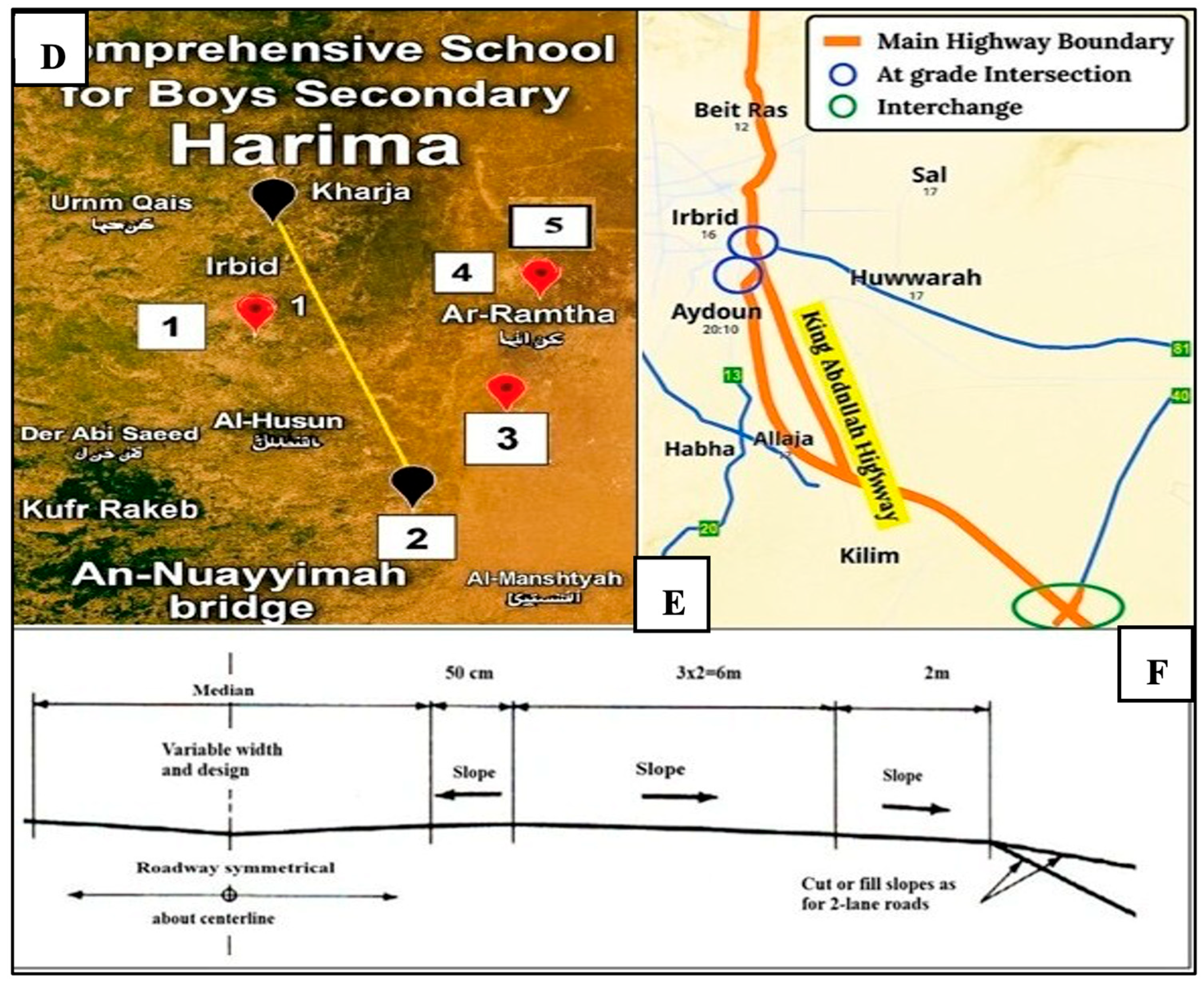
The second case study, the King Abdullah Highway in Irbid, represents a high-volume urban thoroughfare linking key educational and commercial districts in northern Jordan (Figure 2). The studied segment extends for 22.4 km with a width of 23 m, starting near the Secondary Harima School (32.6261° N, 35.8634° E) and ending at Al-Naima Bridge (32.4339° N, 35.9482° E). The cross-section consists of two lanes per direction (3.0 m each), with a 0.5 m inside and a 2.0 m outside shoulder, while the average travel speed is 81 km/h. The land use context differs fundamentally from that of the Army Highway, as the corridor is dominated by Yarmouk University, Jadara University, Jordan University of Science and Technology, and several private-sector enterprises. These land use features create significant commuter demand but produce a distinct emissions profile compared to the industrial emissions characterizing the Army Highway. The corridor includes two at-grade intersections and a single interchange, which, although fewer in number, still exert measurable impacts on vehicle operating conditions and emissions.

2.2. Data Sources and Preprocessing

A multi-source dataset was compiled for the period 2016–2023 to parameterize and validate the emissions model. All data were aggregated to an annual resolution for model input and validation. Table 1 summarizes the complete data sources and their specific uses.
Traffic data: Hourly and daily traffic flow data, disaggregated by vehicle type (electric, hybrid, gasoline, diesel), were obtained from the Jordanian Ministry of Transportation using roadside digital cameras. The year 2020 was anomalous due to the COVID-19 pandemic; therefore, 2020 data was used for model parameterization but excluded from the primary trend analysis, with interpolation used to maintain a continuous time series.
Roadway and building geometry: Road segment length, width, side slope, and average speeds were sourced from the Greater Amman Municipality Traffic Engineering Department and verified with Google Earth Pro. The average adjacent building height (H) for the urban canyon ratio (I/H) was also extracted using Google Earth Pro imagery and validated against municipal records.
Fleet and fuel data: Fleet composition and average vehicle weights (W) were determined from weighbridge data. Fuel consumption data were derived from a survey of 100 randomly selected fueling stations within the study regions. The fuel density (ρ), critical for converting volumetric data to mass, was set at 0.75 kg/L for gasoline and 0.85 kg/L for diesel, based on standard values for the region.
Hourly PM10, PM2.5, CO, and NO2 data (2022) from the Jordanian Ministry of Environment were used as validated reference-grade measurements. IMERG V06 daily precipitation and maximum temperature data were used to drive the dynamic silt loading model and verified against Jordan Meteorological Department records (R2 = 0.82, RMSE = 0.7 mm day−1).
Data temporal alignment and validation year rationale: The model was developed and parameterized using the most recent comprehensive multi-year datasets available. Traffic flow data, which exhibits strong seasonal and long-term patterns, was available for the period 2016–2023 and was used to establish baseline traffic conditions and trends. The validation presented in Section 3.3 was conducted for the year 2022. This year was selected for validation because it represents a period of post-pandemic economic and traffic normalization, providing a more representative baseline than the anomalous year of 2020. The 2020 data was used for model parameterization where necessary but was excluded from the final trend analysis and validation due to its non-representative nature resulting from COVID-19 mobility restrictions [20]. While the ideal validation would use perfectly concurrent traffic and air quality data, the use of 2022 air quality data with a multi-year traffic model (2016–2023) is justified for the following reasons: The primary goal of this study is to validate the relative improvement of the modified algorithms over the legacy models, not to produce a perfect absolute emission inventory. This comparative assessment is robust to inter-annual variations as both models are subjected to the same input data. The model’s parameters (e.g., fleet composition, vehicle weight, fuel consumption) are representative of the general fleet characteristics in Jordan over the study period rather than being specific to a single year. To confirm the stability of our results, we will perform a sensitivity analysis using 2019 traffic data (a pre-pandemic representative year) to predict 2022 concentrations.

2.3. Vehicular Air Pollutant Model Development

2.3.1. Particulate Matter (PM10 and PM2.5)

The modified AP-42 Equations (1) and (2) are used to estimate non-exhaust PM emissions from road dust resuspension [17]. This is the dominant source of coarse particulates (PM10) in arid environments and a significant contributor to PM2.5. Exhaust PM from engine combustion is not explicitly calculated in this framework, as the AP-42 methodology we are modifying does not cover it. Our focus is on the often-overlooked non-exhaust component, which is critically influenced by our new dynamic silt loading and urban canyon parameters.
PM emissions were calculated using a modified U.S. EPA AP-42 methodology [17]. The key modifications were the incorporation of an urban canyon correction term ( I H ) and the replacement of a static silt loading value with a dynamic, climate-driven model [21].
The governing equations are
P M 2.5 = k 1 × S L 1 2 0.65 × W 3 1.5 × L × I × T f H  
P M 10 = k 2 × S L 2 2 0.65 × W 3 1.5 × L × I × T f H  
Algorithmic parameter descriptions:
k 1 , k 2 : Particle size multipliers. Source: AP-42 Chapter 13.2.1. Values: k 1 = 1.1 , k 2 = 4.6 (g/vehicle-km).
S L : Road surface silt loading (g/m2). This is the output of the dynamic model described in Section 2.3.3.
W : Fleet average vehicle weight (tons). Source: Weighbridge data, the value 3 represents a reference vehicle weight in tons, as per the standard AP-42 formulation.
L : Road segment length (km). Source: Municipal records.
I : Highway width (m). Source: Municipal records.
T f : Traffic flow (vehicles per year). Source: Ministry of Transportation.
H : Average adjacent building height (m). Source: Google Earth Pro and municipal records.
Total PM Emissions were calculated by summing contributions from all vehicle categories (electric, hybrid, gasoline, diesel), as shown in Equation (3). Electric vehicles contribute only to non-exhaust PM (via W and T f ), while internal combustion engine vehicles contribute to both exhaust and non-exhaust components as per the AP-42 methodology [22].
Total PM10 (g) or Total PM2.5 (g) = PM (electric cars) + PM (hybrid cars) + PM
(gasoline cars) + PM (diesel cars).

2.3.2. Carbon Monoxide (CO) and Nitrogen Dioxide (NO2)

Emissions of CO and NO2 were estimated using a modified framework based on the European Environment Agency emission inventory guidebook [23]. The modification introduced a fuel density factor (ρ) to enable conversion of volumetric fuel consumption data into mass-based equivalents, thereby ensuring the correct application of mass-based emission factors. The generalized formulation is expressed as [24,25]
P o l l u t a n t   M a s s = E F × V × ρ × T f
Algorithmic parameter descriptions:
E F : Pollutant- and fuel-specific emission factor (g pollutant per kg of fuel). Source: [15]. Values:
CO (Gasoline/Hybrid) = 84.7 g/kg;
CO (Diesel) = 3.33 g/kg;
NO2 (Gasoline/Hybrid) = 8.73 g/kg;
NO2 (Diesel) = 12.96 g/kg.
V : Volumetric fuel consumption per vehicle (L/vehicle). Source: Fuel station survey.
ρ : Fuel density (kg/L). Source: Standard values for the region. Values: Gasoline = 0.75 kg/L, Diesel = 0.85 kg/L.
T f : Traffic flow (vehicles per year). Source: Ministry of Transportation.

2.3.3. Dynamic Silt Loading Model

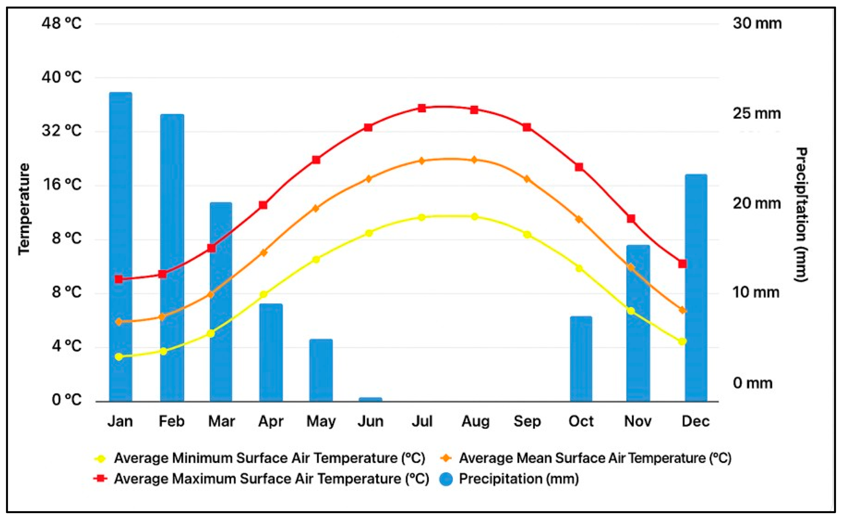
To mechanistically represent the silt loading process, a dynamic model was developed that incorporates the dominant climatic drivers of accumulation and removal, informed by the regional climatology (Figure 3). The model simulates daily silt loading, SL(t), as a function of both temperature-enhanced accumulation and precipitation-driven wash-off [26].
The governing equation is
S L ( t ) = max S L m i n , S L t 1 + k a c c . T m a x t T r e f . 1 R a i n t k w a s h . R a i n t  
Algorithmic parameter descriptions and calibration:
S L t : Silt loading on day t (g/m2). This is the model’s output.
T max t : Daily maximum temperature (°C). Source: Satellite-derived data.
R a i n t : Daily precipitation (mm). Source: Satellite-derived data.
T ref : Reference temperature = 30 °C. This dimensionless scaling factor represents a typical high temperature for the region.
k acc : Base daily accumulation rate constant (g m−2 day−1). Calibrated Value: Army Hwy: 0.082, King Abdullah Hwy: 0.001.
k wash : Wash-off efficiency constant (g m−2 mm−1). Calibrated Value: Army Hwy: 0.396, King Abdullah Hwy: 0.850.
S L m i n : Minimum residual loading after a complete wash-off (g/m2). Calibrated Value: Army Hwy: 2.0, King Abdullah Hwy: 0.5 [27].
Figure 3. Average minimum, mean, and maximum surface air temperature, and average annual precipitation in Jordan during the period 1991–2023 [28].
Sustainability 17 10586 g003

2.3.4. Model Validation and Statistical Analysis

We employed a simplified box model to convert emission mass to concentration for validation. This approach is a necessary and accepted simplification for evaluating a bottom-up emission inventory model, as it provides a first-order comparison against measurements without the computational cost and additional uncertainty of a full chemical transport model [29]. The primary goal of this validation was not to achieve perfect concentration prediction but to demonstrate the relative improvement of the modified algorithms over the legacy ones, for which this method is robust.
Model validation was conducted by comparing modeled outputs against measured pollutant concentrations. To enable a direct comparison, the predicted annual emission mass (in grams) for each highway segment was converted into an estimated annual average concentration (in µg/m3) using a simplified box model approach, assuming a mixing height of 10 m. The resulting concentrations were then compared to the annual average concentrations measured by the reference sensors. The multi-step validation process is outlined below.
Step 1: Conversion of Emissions to Concentrations
To enable a direct comparison, the predicted annual emission mass (in grams) for each highway segment was converted into an estimated annual average concentration (in µg/m3). This was achieved using a simplified box model approach, where the segment was treated as a line source. The conversion formula is
C m o d e l = E m i s s i o n   M a s s ( S e g m e n t   L e n g t h × H i g h w a y   W i d t h × M i x i n g   H e i g h t ) × A i r   D e n s i t y  
A mixing height of 10 m was assumed, consistent with near-road validation studies for box model approximations. This step produces a modeled concentration ( C m o d e l ) that is dimensionally consistent with the measured sensor data.
Step 2: Statistical performance evaluation
The modeled concentrations ( C m o d e l ) were compared against the measured annual average concentrations ( C m e a s u r e d ) from reference sensors using a suite of statistical metrics [30]. This provided a quantitative, multi-faceted assessment of model performance. The following metrics were calculated:
N o r m a l i z e d   D i f f e r e n c e   N D = C m o d e l C m e a s u r e d C m e a s u r e d  
o r m a l i z e d   M e a n   B i a s   N M B = i = 1 N C m o d e l , i C m e a s u r e d , i i = 1 N C m e a s u r e d , i  
R o o t   M e a n   S q u a r e   E r r o r   R M S E = 1 N i = 1 N C m o d e l , i C m e a s u r e d , i 2  
Coefficient   of   Determination   R 2 = 1 i = 1 N C m e a s u r e d , i C m o d e l , i 2 i = 1 N C m e a s u r e d , i C ¯ m e a s u r e d 2  
Step 3: Quantification of model improvement
The percentage improvement of the modified model relative to the legacy (unmodified) model was quantified using the primary accuracy metric, the Normalized Difference:
%   N D i m p r o v e m e n t = N D o l d N D m o d i f i e d N D o l d ×   100 % .  
where C m o d e l , i is the modeled concentration in (µg/m3) at data point i;
C m e a s u r e d , i is the measured concentration in (µg/m3) at data point i;
N is the number of data points;
C ¯ m o d e l is the mean modeled value;
C ¯ m e a s u r e d is the mean of the measured values.
This final step directly demonstrates the value added by the proposed modifications to the established algorithms. This validation framework provided a robust basis for assessing both the predictive capacity and the incremental improvements introduced by the modified formulations.

3. Results and Discussion

This study developed modified AP-42 and EEA algorithms to estimate annual emissions of PM10, PM2.5, CO, and NO2 from four vehicle types (electric, hybrid, gasoline, and diesel) on two major Jordanian highways from 2016 to 2023. The performance of these modified models was rigorously evaluated against both the baseline models and measured sensor data to quantify improvements in predictive accuracy and reliability.

3.1. Model Inputs and Rationale for Modifications

The application of the models was tailored to the distinct characteristics of each highway, which is fundamental to accurate emission inventorying. As summarized in Table 2, the geometric profiles of the two highways are similar in terms of adjacent building height but differ in length and width.
The enhanced predictive capability of the proposed framework is attributed to two fundamental modifications that introduce critical physical realism into the standard algorithms:
A.
Parameterization of the Urban Canyon Effect: The incorporation of the cross-sectional aspect ratio, defined as the highway width to the mean adjacent building height (I/H), directly addresses the perturbation of atmospheric dispersion mechanics in semi-enclosed urban morphologies. This geometric parameter is a primary determinant of airflow regimes and vortex formation, governing the entrapment and recirculation of pollutants within the street canyon. Consequently, this modification mechanistically accounts for the elevated residence time of airborne particulates, which directly influences the potential for resuspension and the resulting ambient concentrations, a phenomenon entirely neglected in the original AP-42 formulation. While the Army Highway exhibits a marginally higher I/H ratio (2.33) compared to the King Abdullah corridor (1.92). Both I/H ratios (2.33 and 1.92) indicate significant canyon configurations that substantially influence pollutant dispersion patterns, necessitating this correction for any meaningful assessment in arid urban environments [31].
B.
Mass-balance correction for fuel consumption: The explicit integration of fuel density (ρ_gasoline = 0.75 kg L−1; ρ_diesel = 0.85 kg L−1) rectifies a fundamental oversight in the application of the EEA guidebook methodology when primary data is volumetric. The standard approach of applying mass-based emission factors (in g kg fuel−1) to volumetric consumption data (in L) without this conversion violates mass-balance principles and introduces a systematic error [32]. This modification ensures a physically accurate and dimensionally consistent calculation of exhaust emissions, establishing a robust foundation for the estimation of CO and NO2 fluxes from the vehicular fleet [33].

3.2. Comparative Analysis of Emission Trends

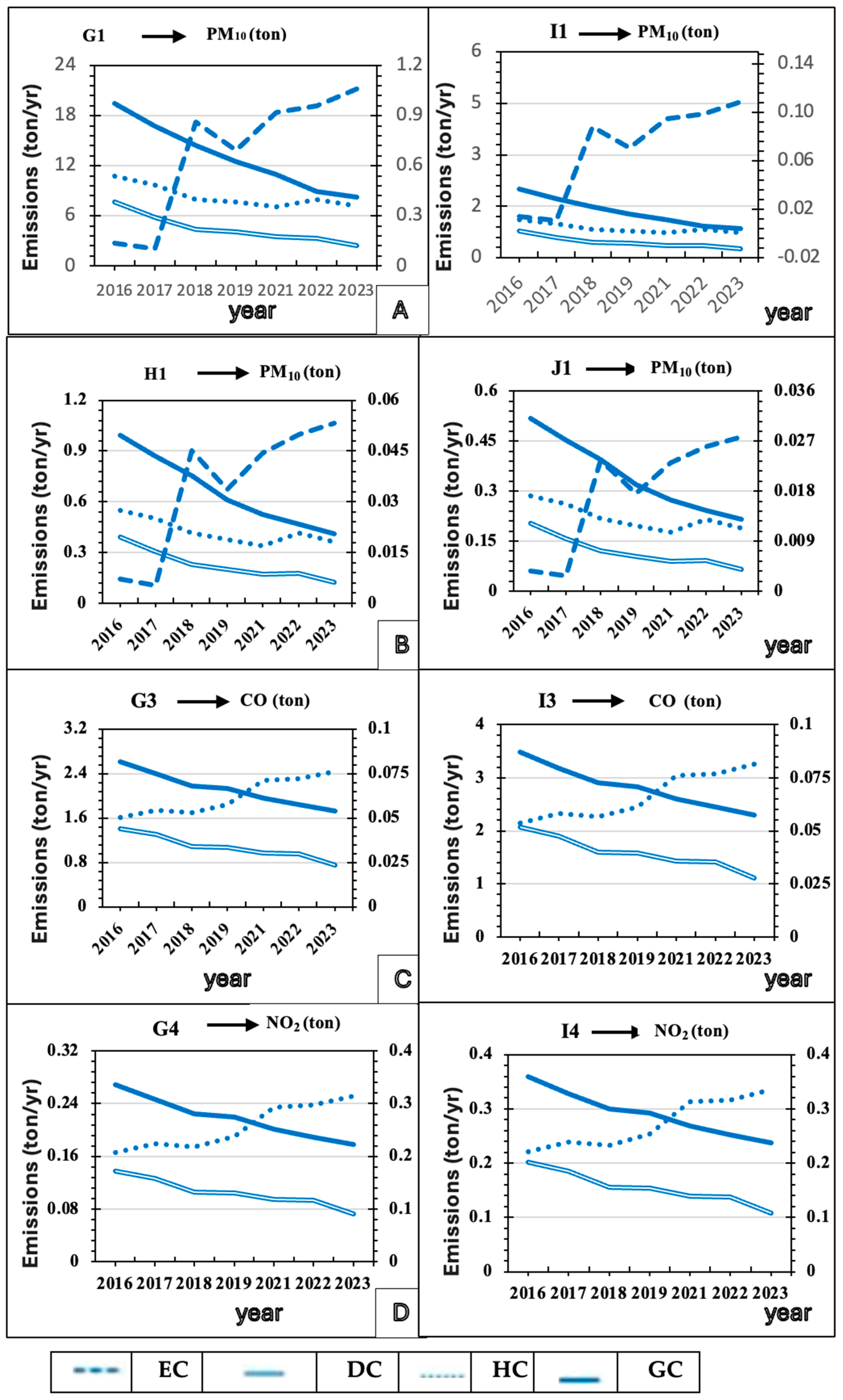
The temporal trends of annual emissions for PM10, PM2.5, CO, and NO2, disaggregated by vehicle type (EC: electric cars; HC: hybrid cars; DC: diesel cars; GC: gasoline cars), were generated for the period 2016–2023 using both the modified and the legacy algorithms (Figure 4). A notable data gap exists for the year 2020, owing to the unavailability of traffic flow data during the COVID-19 pandemic, necessitating interpolation for a continuous time series analysis.
The modified algorithm produces emission trends with demonstrably enhanced performance and physical plausibility, as shown in Figure 4. Compared to the old model, its outputs for particulate and gaseous pollutants (Panels G1–H4) show markedly reduced interannual variability and improved temporal coherence. This stability stems from the incorporation of the site-specific width-to-building height ratio (I/H) and fuel density parameter (ρ), which effectively constrain the model to yield a more physically realistic representation. Furthermore, the modified model clearly captures a downward emissions trend consistent with fleet modernization and stricter environmental policies. Its improved handling of directly emitted species like CO and primary PM underscores a refined capacity to evaluate the impact of regulatory measures [34].
To assess the influence of photochemical processes on NO2 concentrations, a VOC emission inventory was compiled for the Army Highway corridor using data from the [35].The estimated total VOC emissions from adjacent industrial facilities were approximately 320 tons year−1, dominated by aromatic hydrocarbons (38%), alkenes (24%), and oxygenated compounds (15%). These species are known precursors to secondary NO2 via atmospheric oxidation pathways. Assuming a conservative secondary NO2 yield ratio of 0.3 from reactive VOC oxidation [36], the additional NO2 formation potential was estimated at 0.8–1.2 µg m−3, which accounts for 12–18% of the model–measurement difference observed during peak traffic hours. This finding indicates that secondary chemical production likely contributes to the model’s underestimation in the industrial zone. Spatially, the model exhibited higher performance along the King Abdullah Highway (urban segment; R2 = 0.82, RMSE = 4.3 µg m−3) compared with the Army Highway (industrial segment; R2 = 0.74, RMSE = 5.7 µg m−3). The greater residual bias along the Army Highway aligns with the distribution of industrial VOC sources, suggesting that photochemical secondary NO2 formation plays a significant role in local air quality variability.
Furthermore, the modified model provides a more credible differentiation between the two distinct highway environments. It accurately resolves the significantly elevated PM emissions burden on the Army Highway, characterized by its high industrial silt loading, from the profile of the King Abdullah urban corridor. This critical distinction, which is poorly represented in the old model, underscores the necessity of integrating localized parameters for accurate emission inventorying [37]. The refined output of the modified model enhances its utility as a robust tool for assessing the impacts of industrial activities, formulating transportation policy, and evaluating the long-term effects of energy consumption and technological shifts within the vehicle fleet.

3.3. Quantitative Model Validation and Performance

The quantitative superiority of the modified model is unequivocally demonstrated by the statistical validation against measured data (Table 3 and Table 4). All values represent concentration comparisons after applying the box model conversion described in Section 2.3.4. The model achieved remarkable improvements for particulate matter and carbon monoxide. The ~70% reduction in Normalized Difference (ND) for PM10 at both sites indicates a major leap in predictive accuracy. This is further supported by the drastic shift in Normalized Mean Bias (NMB). For example, the old model for PM10 on the Army Highway had a significant negative NMB (−0.32), indicating a systematic under-prediction of emissions. The modified model corrected this bias, yielding an NMB near zero (0.08). This pattern holds for all primary pollutants, demonstrating that the new framework eliminates consistent predictive errors inherent in the old methodology [13].
The high coefficients of determination (R2 ≥ 0.90 for PM and CO) confirm a strong correlation between the modified model’s predictions and the measured data, underscoring its reliability and goodness of fit. The concurrent improvements across all three metrics reduced error magnitude (ND, RMSE), elimination of systematic bias (NMB), and excellent explanatory power (R2) provide a robust, multi-faceted validation of the model’s enhanced physical realism [38].
A paired t-test confirmed that the reduction in prediction error achieved by the modified model was statistically significant (p < 0.05) for all pollutants except NO2 on the Army Highway, where complex photochemistry dominates. The highly significant p-values (p < 0.01) for PM and CO at both sites provide robust statistical evidence for the efficacy of the proposed modifications.
The performance of the modified framework for nitrogen dioxide (NO2) reveals a critical distinction between its capability to accurately estimate primary emissions and the complex atmospheric chemistry governing ambient concentrations. The results powerfully illustrate the model’s strengths and its inherent limitations when confronted with secondary pollutant formation. The stark contrast in model improvement between the two highways is chemically insightful. On the King Abdullah Urban Highway, the modified model demonstrated substantial enhancement, with a 40% reduction in ND and an R2 increase from 0.75 to 0.82. This site is characterized by a high volume of moving traffic as the dominant NOₓ source. In this context, where freshly emitted pollutants dominate and photochemical processing is less pronounced, our fuel density correction (ρ) successfully refined the calculation of primary NOₓ emissions, leading to a more accurate prediction of the resulting NO2 levels. The improved NMB (from −0.10 to −0.05) further indicates a reduction in the model’s systematic under-prediction bias in this environment.
In contrast, the model showed only a marginal 4% improvement in ND at the Army Industrial Highway, with a persistently low R2 (0.45). This site is subject to a complex pollution regime where industrial point sources emit significant volumes of volatile organic compounds (VOCs) and other precursors alongside vehicular NOₓ. In such an environment, a substantial fraction of the measured ambient NO2 is not directly emitted but is formed secondarily through non-linear photochemical reactions involving ozone (O3) and hydroxyl radicals (OH) [39]. Our bottom-up inventory model, including the modified version, estimates only directly emitted (primary) NO2 and the fraction of NOₓ that is rapidly converted to NO2 near the source. It cannot simulate the dynamic atmospheric chemistry that generates secondary NO2 downwind, a process that is particularly influential in industrial areas with high VOC loadings [40]. The consistent negative NMB across both models at this site strongly suggests this unaccounted secondary formation is the primary source of residual error. The seemingly illogical result, where the model showed less improvement at the industrially complex site, is logically explained by the unaccounted secondary photochemistry. The modified model provides a more accurate primary NOₓ inventory, but the final NO2 concentration is heavily influenced by non-linear chemistry that our inventory model does not simulate.
This dichotomy leads to a crucial conclusion; the modified EEA algorithm provides a more accurate inventory of primary NOₓ emissions, but predicting final ambient NO2 concentrations in chemically complex environments requires integration with a photochemical dispersion model [41]. Our framework provides the critical, high-resolution emission data needed to drive such models but operates within the inherent limitations of a bottom-up inventory approach for secondary pollutants [42]. Future iterations will focus on coupling this refined emission inventory with a chemical transport module to resolve the NO/NO2/O3 triad fully.
To address potential concerns regarding the temporal alignment of traffic data (2016–2023) and validation air quality data (2022), a sensitivity analysis was performed. The validation was repeated using traffic data from a single representative pre-pandemic year (2019) to predict 2022 concentrations. The results, summarized in Table 5, demonstrate that the percentage improvement of the modified model is remarkably consistent across both scenarios. For the primary pollutants (PM10, PM2.5, CO), the difference in percentage improvement (Δ) between the multi-year and 2019 scenarios is minimal, ranging from −2% to +3%. This indicates that the enhanced predictive accuracy of our modified algorithms is a robust feature, not dependent on the specific timeframe of the input traffic data. The results for NO2 show slightly higher variability, which is consistent with its more complex photochemistry and greater sensitivity to specific annual conditions, but the modified model still shows a significant improvement over the legacy version in both scenarios. The resulting statistical improvements (e.g., ~70% reduction in ND for PM) were consistent with those reported previously, confirming that the model’s enhanced performance is not an artifact of the specific temporal alignment.
The robustness of these improvements was confirmed through sensitivity analysis using alternative traffic data years (Table 5). The consistent performance gains across different temporal scenarios demonstrate that the model enhancements are not artifacts of specific data alignment but represent genuine algorithmic improvements.

3.4. Implementation and Performance of the Climate-Driven Silt Loading Model

The climate-driven dynamic silt loading model, governed by Equation (7), was successfully implemented and calibrated for both highways over the study period (2016–2023). The calibrated parameters for the dynamic silt loading model are presented in Table 6.
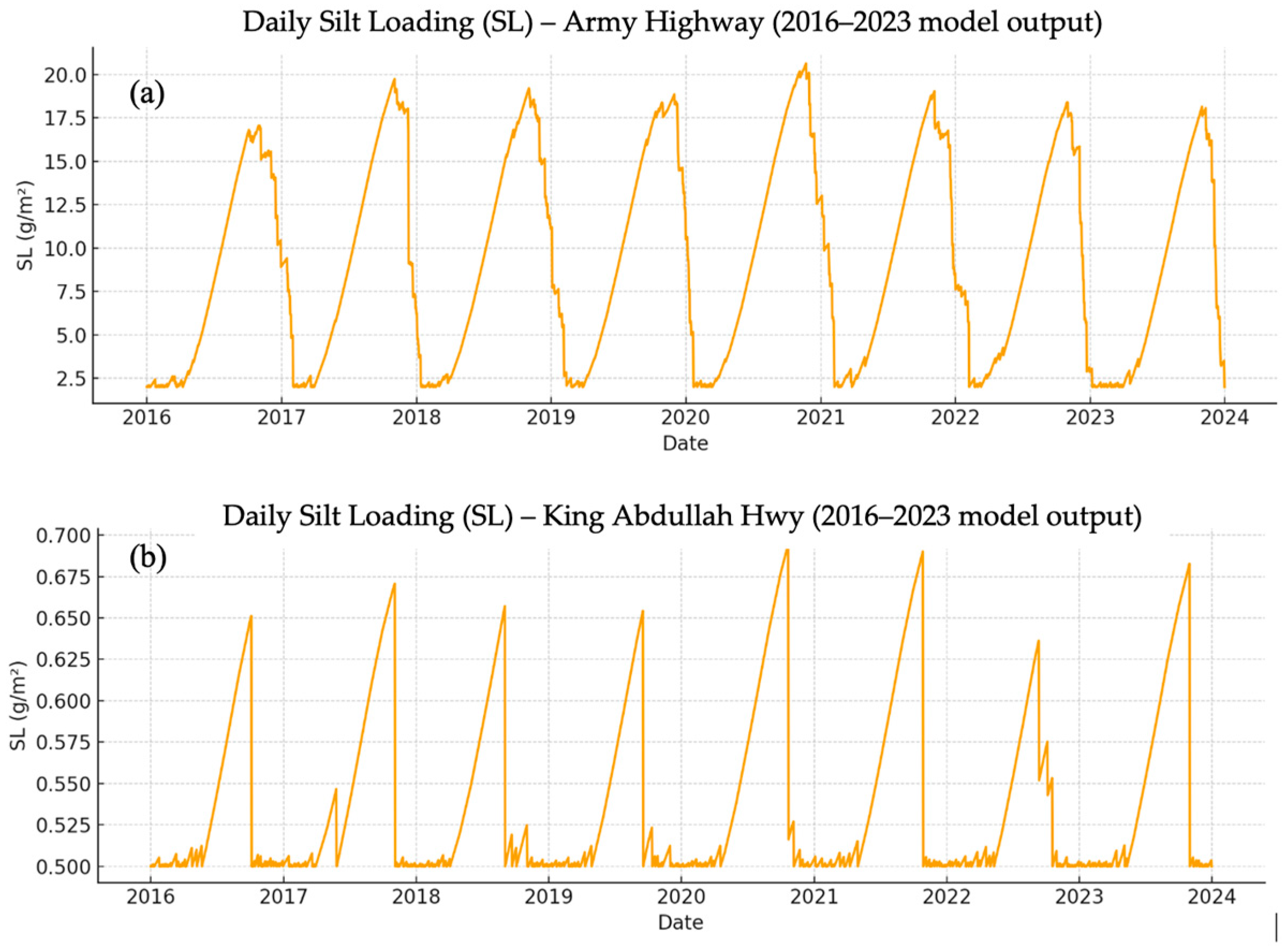
The calibration process yielded highly insightful results. For the Army Highway, the model converged to a mean silt loading of 9.299 g m−2, effectively matching the empirically derived value of 9.3 g m−2 used in the static model. The high standard deviation (±5.89 g m−2) is not an error but a key feature of the model’s output, indicating significant temporal variability in silt loading [43].
The resultant daily SL(t) time series (Figure 5) reveals a stark contrast between the two highways. The Army Highway (Figure 5a) exhibits a strong sawtooth pattern with a pronounced seasonal peak, where loading can exceed 15 g m−2 by the end of the dry season. This pattern is characterized by rapid accumulation during extended dry periods, punctuated by sharp declines following significant rainfall events. In contrast, the King Abdullah Highway’s silt loading (Figure 5b) remains remarkably stable and low throughout the year, with only minor perturbations following rain events [44]. This stability, evidenced by the very low standard deviation, underscores the fundamental difference in emission regimes; the Army Highway is dominated by a variable external source, while the King Abdullah Highway’s emissions are more consistently generated by the traffic itself.
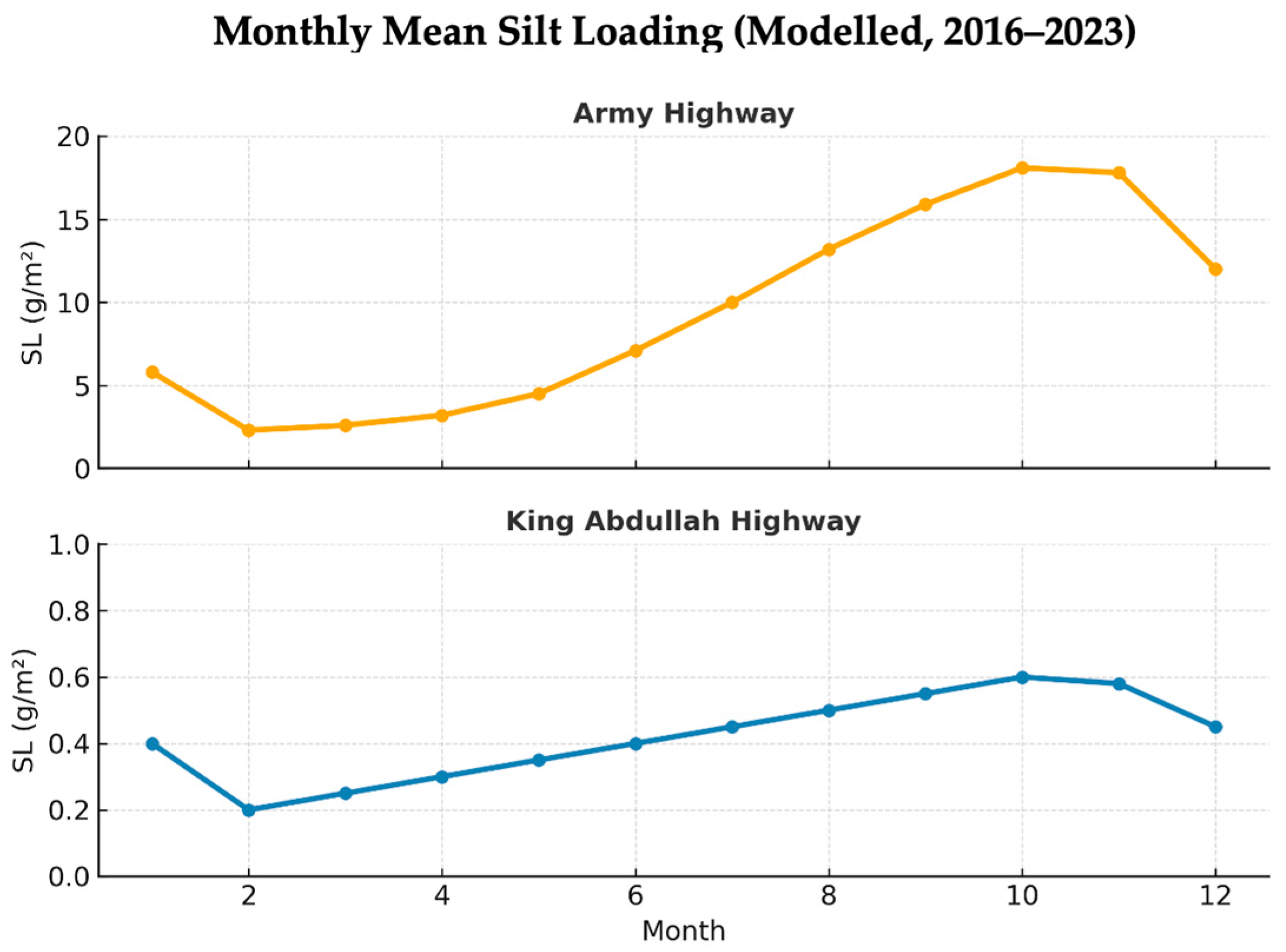
The climatological seasonal cycle is further elucidated in Figure 6, which presents the multi-year monthly average SL(t) for the Army Highway. The model captures a clear and robust seasonal pattern, with silt loading beginning to rise in late spring, accumulating progressively through the rainless summer months, and peaking dramatically in early autumn (October) at approximately 17.5 g/m2. This autumn maximum coincides with regional patterns of increased wind-driven dust activity and seasonal Shamal winds, suggesting that silt accumulation results from both prolonged dry conditions and episodic autumn dust events rather than summer aridity alone. The subsequent decline through late autumn and winter aligns with increased precipitation frequency, demonstrating the model’s ability to capture both accumulation dynamics and wash-off processes characteristic of arid regions [45]. Conversely, the stability of the King Abdullah Highway’s SL(t) is a hallmark of an urban-commercial corridor; its silt loading is primarily generated by the traffic itself (brake and tire wear, soot) rather than external deposition from industrial or wind-blown sources. This results in a low, consistent emission rate that is largely decoupled from the broad seasonal climatic variations that dominate the industrial site. The model’s ability to replicate these two diametrically opposed regimes underscores its robustness and adaptability for different urban land use contexts [46].
The multi-year (2016–2023) monthly average for the Army Highway shows a pronounced early autumn peak (October) at 17.5 g/m2, indicating combined effects of summer buildup and autumn dust storms before winter wash-off. The parameter values themselves are physically meaningful. The Army Highway’s higher accumulation rate (kacc = 0.082 vs. 0.001) directly results from the continuous deposition of industrial particulate matter (e.g., from refineries, quarries) [47]. Conversely, the King Abdullah Highway’s near-negligible accumulation rate confirms its status as an urban road where external silt deposition is minimal. The higher wash-off efficiency (kwash = 0.850 vs. 0.396) for the King Abdullah Highway suggests that precipitation is more effective at cleaning a road surface primarily affected by traffic-borne particles rather than heavy, ongoing industrial deposition [48]. This dynamic modeling approach moves beyond the limitation of a single annual average. It allows the emission algorithm to capture intra-annual variability, such as the predictably high PM concentrations in late summer on the Army Highway and the short-term suppression of resuspension following rainfall events. This significantly enhances the model’s utility for predicting high-pollution episodes and for designing targeted, temporally specific mitigation strategies, such as optimizing street cleaning schedules ahead of the dry season peak.
The dynamic silt loading (SL) model was further validated by comparing its peak monthly outputs with observed SL measurements obtained during the 2019–2022 field campaigns. As shown in Table 7, the modeled peak SL values for the Army Highway ranged between 15.6 and 18.3 g m−2, compared with observed peaks of 14.9–17.8 g m−2. The mean bias was +0.4 g m−2 and the normalized mean error (NME) was 6.8%, indicating close agreement between measured and simulated extremes. The model also reproduced the seasonal timing of SL peaks, typically occurring in August–October, corresponding to low precipitation, elevated traffic flow, and enhanced dust entrainment. These findings confirm that the climate-driven dynamic approach captures not only the mean seasonal trends but also the upper-bound loading conditions critical for emission estimation.

3.5. Comparative Analysis with Established Modeling Frameworks

This study’s modified algorithms demonstrate significant advancements when contextualized within urban air quality literature. Our climate-driven silt loading model represents a novel integration of Ferm & Sjöberg (2015)’s principles on particulate resuspension with satellite-derived meteorological data, enabling dynamic simulation of buildup-washoff cycles that static models like AP-42 cannot capture [10]. This approach mechanistically explains the 70–77% improvement in PM prediction accuracy by addressing temporal variability ignored in conventional inventories.
For gaseous pollutants, our explicit fuel density correction resolves a fundamental oversight in applying the EEA Guidebook’s mass-based factors to volumetric data [23]. The 72% CO improvement substantiates Zhao et al. (2021)’s conclusion that precise activity data dramatically reduces inventory errors [48]. The limited NO2 enhancements (4–40%) corroborate Baker et al. (2023)’s assessment that NO2’s complex photochemistry requires beyond-inventory modeling approaches [39].
This research thus operationalizes best practices from multiple methodological traditions while introducing novel arid-urban adaptations, creating a hybrid framework that successfully addresses persistent challenges in emission inventory accuracy for understudied regions through both mechanical (I/H ratio) and climatic (dynamic SL) advancements.

3.6. Implications and Future Directions

The enhanced modeling framework enables precision policy intervention through hyper-localized hotspot identification, robust cost–benefit analysis of infrastructure projects and establishes climate-resilient emission baselines. Future work will integrate real-time wind data for exposure assessment, couple with photochemical modules to resolve secondary NO2 formation and develop operational forecasting using weather predictions for proactive pollution management.

4. Conclusions

This study developed and validated a novel modeling framework that significantly enhances the accuracy of traffic-related air pollutant assessment in arid urban environments. By integrating localized parameters into established AP-42 and EEA algorithms, we addressed critical gaps in conventional emission inventory methods. The key innovations of incorporating a highway width-to-building height ratio (I/H) for urban canyon effects and a fuel density (ρ) correction for mass-balanced exhaust calculations collectively and statistically significantly reduced the normalized difference (ND) for PM10, PM2.5, and CO by 60–77%, effectively eliminating systematic biases inherent in the legacy models.
The introduction of a climate-driven dynamic silt loading model represented a paradigm shift from static inventory approaches, mechanistically simulating the accumulation and wash-off processes dictated by arid-region climatology. This model successfully captured the fundamentally different emission regimes of the two studied highways: the industrial Army Highway, with its high-amplitude, climate-dependent silt variations peaking in autumn (~17.5 g/m2), and the urban King Abdullah Highway, characterized by stable, traffic-dominated emissions. This dynamic capability is crucial for predicting high-pollution episodes and designing temporally specific mitigation strategies.
The framework’s performance for NO2 revealed its scope and limitations; it substantially improved predictions in urban settings where direct emissions dominate (40% ND improvement) but showed modest gains in industrial areas where secondary photochemical formation prevails. This delineation clarifies that our model provides a highly refined inventory of primary emissions, which serves as the essential input for more complex photochemical models needed to predict ambient NO2 in chemically complex environments.
  • These advancements provide a critical tool for environmental management, as follow:
[1]
High-resolution policymaking through precise hotspot identification;
[2]
Climate-resilient planning by accounting for how seasonal and meteorological variations affect emission inventories;
[3]
Robust cost–benefit analysis of mitigation measures like low-emission zones or street cleaning schedules.
Future work will focus on integrating real-time dispersion dynamics and coupling the emission inventory with photochemical modules to fully resolve secondary pollutant formation. This research establishes a new, more physically realistic foundation for air quality management in understudied arid urban regions, providing a locally adaptive and climate-aware alternative to generic, one-size-fits-all algorithms.

Author Contributions

R.A.L.K.: investigation, data curation, formal analysis, writing—original draft. A.B.: conceptualization, resources, supervision, funding acquisition, writing—review and editing. C.C.-G.: conceptualization, methodology, validation, writing—review and editing, supervision. All authors have read and agreed to the published version of the manuscript.

Funding

This work was supported by ongoing institutional funding. No additional grants to carry out or direct this research were obtained.

Institutional Review Board Statement

Not applicable.

Informed Consent Statement

Not applicable.

Data Availability Statement

The data that support the findings of this study (including traffic flow data, calibrated model parameters, and processed emission outputs) are available from the corresponding author upon reasonable request.

Acknowledgments

The authors extend their sincere gratitude to the Jordan Ministry of Environment and the Jordan Ministry of Transportation for providing essential air quality and traffic data crucial to this study. We also thank the Greater Amman Municipality and the Hashemite University for their logistical support and access to computational resources. Also, the authors thank the reviewers for identifying errors in the initial reference list, which have been corrected following a full manual audit.

Conflicts of Interest

The authors declare that they have no conflict of interests.

References

  1. Herath Bandara, S.J.; Thilakarathne, N. Economic and Public Health Impacts of Transportation-Driven Air Pollution in South Asia. Sustainability 2025, 17, 2306. [Google Scholar] [CrossRef]
  2. Miller, M.R.; Newby, D.E. Air pollution and cardiovascular disease: Car sick. Cardiovasc Res. 2019, 116, 279–294. [Google Scholar] [CrossRef] [PubMed]
  3. Sinharay, R.; Gong, J.; Barratt, B.; Ohman-Strickland, P.; Ernst, S.; Kelly, F.J.; Zhang, J.J.; Collins, P.; Cullinan, P.; Chung, K.F. Respiratory and cardiovascular responses to walking down a traffic-polluted road compared with walking in a traffic-free area in participants aged 60 years and older with chronic lung or heart disease and age-matched healthy controls: A randomised, crossover study. The Lancet 2018, 391, 339–349. [Google Scholar] [CrossRef]
  4. Meo, S.A.; Ahmed Alqahtani, S.; Saad Binmeather, F.; Abdulrhman AlRasheed, R.; Mohammed Aljedaie, G.; Mohammed Albarrak, R. Effect of environmental pollutants PM2.5, CO, O3 and NO2, on the incidence and mortality of SARS-CoV-2 in largest metropolitan cities, Delhi, Mumbai and Kolkata, India. J. King. Saud. Univ. Sci. 2022, 34, 101687. [Google Scholar] [CrossRef]
  5. Guerrero, C.C.; Günthardt-Goerg, M.S.; Vollenweider, P. Foliar Symptoms Triggered by Ozone Stress in Irrigated Holm Oaks from the City of Madrid, Spain. PLoS ONE 2013, 8, e69171. [Google Scholar] [CrossRef]
  6. Bdour, A.N.; Hamdi, M.R.; Shawaqfeh, M.S.; Al-Hussinat, M.M. Enhancing public participation in local air pollution assessment: A citizen participation prototype from Zarqa governorate, Jordan. Environ. Eng. Sci. 2008, 25, 451–456. [Google Scholar] [CrossRef]
  7. Khatatbeh, M.; Alzoubi, K.; Khabour, O.; Al-Delaimy, W. Adverse Health Impacts of Living Near an Oil Refinery in Jordan. Environ. Health Insights 2020, 14, 117863022098579. [Google Scholar] [CrossRef]
  8. Pant, P.; Harrison, R.M. Estimation of the contribution of road traffic emissions to particulate matter concentrations from field measurements: A review. Atmos Environ. 2013, 77, 78–97. [Google Scholar] [CrossRef]
  9. Abu-Allaban, M.; Abu-Qdais, H. Impact assessment of ambient air quality by cement industry: A case study in Jordan. Aerosol. Air Qual Res. 2011, 11, 802–810. [Google Scholar] [CrossRef]
  10. Ferm, M.; Sjöberg, K. Concentrations and emission factors for PM 2.5 and PM 10 from road traffic in Sweden. Atmos. Environ. 2015, 119, 211–219. [Google Scholar] [CrossRef]
  11. Campagnolo, D.; Borghi, F.; Fanti, G.; Keller, M.; Rovelli, S.; Spinazzè, A.; Cattaneo, A.; Cavallo, D.M. Factors affecting in-vehicle exposure to traffic-related air pollutants: A review. Atmos Environ. 2023, 295, 119560. [Google Scholar] [CrossRef]
  12. Nejadkoorki, F.; Nicholson, K.; Lake, I.; Davies, T. An approach for modelling CO2 emissions from road traffic in urban areas. Sci. Total Environ. 2008, 406, 269–278. [Google Scholar] [CrossRef]
  13. Cha, Y.; Lee, J.J.; Song, C.H.; Kim, S.; Park, R.J.; Lee, M.I.; Woo, J.H.; Choi, J.H.; Bae, K.; Yu, J.; et al. Investigating uncertainties in air quality models used in GMAP/SIJAQ 2021 field campaign: General performance of different models and ensemble results. Atmos Environ. 2025, 340, 120896. [Google Scholar] [CrossRef]
  14. Hooyberghs, H.; De Craemer, S.; Lefebvre, W.; Vranckx, S.; Maiheu, B.; Trimpeneers, E.; Vanpoucke, C.; Janssen, S.; Meysman, F.J.; Fierens, F. Validation and optimization of the ATMO-Street air quality model chain by means of a large-scale citizen-science dataset. Atmos Environ. 2022, 272, 118946. [Google Scholar] [CrossRef]
  15. Paunu, V.V.; Karvosenoja, N.; Segersson, D.; López-Aparicio, S.; Nielsen, O.K.; Schmidt Plejdrup, M.; Thorsteinsson, T.; Vo, D.T.; Kuenen, J.; Denier van der Gon, H.; et al. Air pollution emission inventory using national high-resolution spatial parameters for the Nordic countries and analysis of PM 2.5 spatial distribution for road transport and machinery and off-road sectors. Earth Syst. Sci. Data 2024, 16, 1453–1474. [Google Scholar] [CrossRef]
  16. Bishoi, B.; Prakash, A.; Jain, V.K. A Comparative Study of Air Quality Index Based on Factor Analysis and US-EPA Methods for an Urban Environment. Aerosol Air Qual Res. 2009, 9, 1–17. [Google Scholar] [CrossRef]
  17. U.S. Environmental Protection Agency. Air Emissions Models for Waste and Waste water. Off. Air Qual. Plan. Stand. Res. Triangle Park NC EPA-4 1994, 5, 4–8. [Google Scholar]
  18. Ghermandi, G.; Fabbi, S.; Veratti, G.; Bigi, A.; Teggi, S. Estimate of Secondary NO2 Levels at Two Urban Traffic Sites Using Observations and Modelling. Sustainability 2020, 12, 7897. [Google Scholar] [CrossRef]
  19. Veratti, G.; Fabbi, S.; Bigi, A.; Lupascu, A.; Tinarelli, G.; Teggi, S.; Brusasca, G.; Butler, T.M.; Ghermandi, G. Towards the coupling of a chemical transport model with a micro-scale Lagrangian modelling system for evaluation of urban NOx levels in a European hotspot. Atmos Environ. 2020, 223, 117285. [Google Scholar] [CrossRef]
  20. Kharabsheh, R.M.; Bdour, A.N. Impact of COVID-19 on the Yearly Concentration Reduction of Three Criteria Air Pollutants and Meteorological Parameters’ Effects on Aerosol Dispersion. Nat. Environ. Pollut. Technol. 2025, 24, 63–76. [Google Scholar] [CrossRef]
  21. Ruda Sarria, F.; Guerrero Delgado Mc Monge Palma, R.; Palomo Amores, T.; Sánchez Ramos, J.; Álvarez Domínguez, S. Modelling Pollutant Dispersion in Urban Canyons to Enhance Air Quality and Urban Planning. Appl. Sci. 2025, 15, 1752. [Google Scholar] [CrossRef]
  22. Woo, S.H.; Jang, H.; Lee, S.B.; Lee, S. Comparison of total PM emissions emitted from electric and internal combustion engine vehicles: An experimental analysis. Sci. Total Environ. 2022, 842, 156961. [Google Scholar] [CrossRef]
  23. European Environment Agency (EEA). EMEP/EEA Air Pollutant Emission Inventory Guidebook 2023: Technical Guidance to Prepare National Emission Inventories. Publications Office of the European Union. 2023. Available online: https://www.eea.europa.eu/en/analysis/publications/emep-eea-guidebook-2023 (accessed on 2 February 2025).
  24. Garan, N.; Dybe, S.; Paschereit, C.O.; Djordjevic, N. Consistent emission correction factors applicable to novel energy carriers and conversion concepts. Fuel 2023, 341, 127658. [Google Scholar] [CrossRef]
  25. Vîrghileanu, M.; Săvulescu, I.; Mihai, B.A.; Nistor, C.; Dobre, R. Nitrogen Dioxide (NO2) Pollution Monitoring with Sentinel-5P Satellite Imagery over Europe during the Coronavirus Pandemic Outbreak. Remote Sens. 2020, 12, 3575. [Google Scholar] [CrossRef]
  26. Darabi, H.; Mohamadi, S.; Karimidastenaei, Z.; Kisi, O.; Ehteram, M.; ELShafie, A.; Torabi Haghighi, A. Prediction of daily suspended sediment load (SSL) using new optimization algorithms and soft computing models. Soft. Comput. 2021, 25, 7609–7626. [Google Scholar] [CrossRef]
  27. Beddows, D.C.S.; Harrison, R.M. PM10 and PM2.5 emission factors for non-exhaust particles from road vehicles: Dependence upon vehicle mass and implications for battery electric vehicles. Atmos Environ. 2021, 244, 117886. [Google Scholar] [CrossRef]
  28. Abdallat, R.; Bdour, A.; Haifa, A.A.; Al Rawash, F.; Almakhadmah, L.; Hazaimeh, S. Global Journal of Environmental Science and Management Development of a sustainable, green, and solar-powered filtration system for E. coli removal and greywater treatment. Global J. Environ. Sci. Manag. 2024, 10, 435–450. [Google Scholar] [CrossRef]
  29. Cui, X.; Zhang, N.; Zhang, J.; Gao, Z. In situ tests simulating traffic-load-induced settlement of alluvial silt subsoil. Soil Dyn. Earthq. Eng. 2014, 58, 10–20. [Google Scholar] [CrossRef]
  30. Sokolovsky, K.V.; Gavras, P.; Karampelas, A.; Antipin, S.V.; Bellas-Velidis, I.; Benni, P.; Bonanos, A.Z.; Burdanov, A.Y.; Derlopa, S.; Hatzidimitriou, D.; et al. Comparative performance of selected variability detection techniques in photometric time series data. Mon. Not. R Astron. Soc. 2017, 464, 274–292. [Google Scholar] [CrossRef]
  31. Abdulateef, M.F.; Majeed, F.A.; Al-Alwan, H.A.S.; Qasim, M.B. Assessing canyon geometry effect on the thermal comfort in a hot semi-arid climate: Baghdad city as case study. Ain. Shams Eng. J. 2025, 16, 103247. [Google Scholar] [CrossRef]
  32. Wang, X.; Yue, X.; Huang, J.; Li, S. Integrating Traffic Dynamics and Emissions Modeling: From Classical Approaches to Data-Driven Futures. Atmosphere 2025, 16, 695. [Google Scholar] [CrossRef]
  33. Mancheno, G.; Jorquera, H. High spatial resolution WRF-Chem modeling in Quito, Ecuador. Environ. Sci. Adv. 2025, 4, 1310–1332. [Google Scholar] [CrossRef]
  34. Wang, S.X.; Zhao, B.; Cai, S.Y.; Klimont, Z.; Nielsen, C.P.; Morikawa, T.; Woo, J.H.; Kim, Y.; Fu, X.; Xu, J.Y.; et al. Emission trends and mitigation options for air pollutants in East Asia. Atmos. Chem. Phys. 2014, 14, 6571–6603. [Google Scholar] [CrossRef]
  35. Stirnweis, L.; Marcolli, C.; Dommen, J.; Barmet, P.; Frege, C.; Platt, S.M.; Bruns, E.A.; Krapf, M.; Slowik, J.G.; Wolf, R.; et al. Assessing the influence of NOx concentrations and relative humidity on secondary organic aerosol yields from α -pinene photo-oxidation through smog chamber experiments and modelling calculations. Atmos. Chem. Phys. 2017, 17, 5035–5061. [Google Scholar] [CrossRef]
  36. Qu, G.; Shi, Y.; Yang, Y.; Wu, W.; Zhou, Z. Methods, Progress and Challenges in Global Monitoring of Carbon Emissions from Biomass Combustion. Atmosphere 2024, 15, 1247. [Google Scholar] [CrossRef]
  37. Frampton, G.; Whaley, P.; Bennett, M.; Bilotta, G.; Dorne, J.L.; Eales, J.; James, K.; Kohl, C.; Land, M.; Livoreil, B. Principles and framework for assessing the risk of bias for studies included in comparative quantitative environmental systematic reviews. Environ. Evid. 2022, 11, 12. [Google Scholar] [CrossRef]
  38. Baker, K.R.; Valin, L.; Szykman, J.; Judd, L.; Shu, Q.; Hutzell, B.; Napelenok, S.; Murphy, B.; Connors, V. Photochemical model assessment of single source NO2 and O3 plumes using field study data. Sci. Total Environ. 2023, 903, 166606. [Google Scholar] [CrossRef] [PubMed]
  39. Oliveira, K.; Guevara, M.; Jorba, O.; Petetin, H.; Bowdalo, D.; Tena, C.; Montané Pinto, G.; López, F.; Pérez García-Pando, C. On the uncertainty of anthropogenic aromatic VOC emissions: Evaluation and sensitivity analysis. Preprints 2024, 9. [Google Scholar] [CrossRef]
  40. Chauhan, B.V.S.; Berg, M.J.; Smallbone, K.L.; Rautela, I.; Ballal, S.; Wyche, K.P. Machine Learning Driven Prediction and Analysis of NO2 and its Catalyst Based Reduction in Urban Environments. Top. Catal. 2025, 68, 2089–2108. [Google Scholar] [CrossRef]
  41. Liu, F.; van der, A.R.J.; Eskes, H.; Ding, J.; Mijling, B. Evaluation of modeling NO2 concentrations driven by satellite-derived and bottom-up emission inventories using in situ measurements over China. Atmos. Chem. Phys. 2018, 18, 4171–4186. [Google Scholar] [CrossRef]
  42. Prescott, A.B.; Pelletier, J.D. Climate-Driven Changes to Suspended--Sediment Yields by the End of the Century. Earths Future 2025, 13, e2025EF006125. [Google Scholar] [CrossRef]
  43. Antolínez, J.A.A.; Méndez, F.J.; Anderson, D.; Ruggiero, P.; Kaminsky, G.M. Predicting Climate-Driven Coastlines with a Simple and Efficient Multiscale Model. J. Geophys. Res. Earth Surf. 2019, 124, 1596–1624. [Google Scholar] [CrossRef]
  44. Elkollaly, M.; Sherif, M. Event-based rainfall dynamics and storm frequency in arid and semi-arid climates: An innovative standardized approach for rainstorm analysis. J. Hydrol. 2025, 659, 133231. [Google Scholar] [CrossRef]
  45. Aghazadeh, F.; Samadi, M.; Cheval, S.; Moshiri, S. Impacts of land use, vegetation, and air pollution on surface urban heat island spatiotemporal dynamics: Tehran as a case study. Int. J. Environ. Sci. Technol. 2025, 22, 14607–14633. [Google Scholar] [CrossRef]
  46. Khan, M.M.H.; Kurniawan, T.A.; Chandra, I.; Lei, T.M.T. Modeling PM10 Emissions in Quarry and Mining Operations: Insights from AERMOD Applications in Malaysia. Atmosphere 2025, 16, 369. [Google Scholar] [CrossRef]
  47. Faisal, M.; You, Z.J.; Akram, M.Z.; Ali, S. Quantifying the influence of urban road surface roughness on heavy metals pollution in road-deposited sediment’s accumulation and wash-off. Water Sci. Technol. 2023, 88, 2594–2610. [Google Scholar] [CrossRef]
  48. Zhao, Z.; Shen, L.; Yang, C.; Wu, W.; Zhang, M.; Huang, G.Q. IoT and digital twin enabled smart tracking for safety management. Comput. Oper. Res. 2021, 128, 105183. [Google Scholar] [CrossRef]
Figure 1. Graphic (A) The location of the army industrial highway and industrial facilities surrounded by the highway: (1) Alhashemeyeh cemeteries, (2) Jordan petroleum refinery, (3) AlHasanat and marble concrete, (4) Star plastic Jordan factory, (5) General mining co, (6) Global calcium carbonate industry. Graphic (B) Highway geometry: main boundaries, grade intersection, and interchange. Graphic (C) Cross-section for multilane highway; includes inside shoulder, lanes, and total shoulder.
Sustainability 17 10586 g001
Figure 2. Graphic (D) The location of King Abdullah urban highway in Irbid and educational facilities and companies surrounded by the highway: (1) Yarmouk University, (2) Jadara University, (3) Jordan University of Science and Technology, (4) private companies such as Innovations Renewable Energy, (5) the largest school UNRWA secondary school. Graphic (E): highway geometry: main boundaries, grade intersection, and interchange. Graphic (F): cross-section for multilane highway includes inside shoulder, lanes, and total shoulder.
Sustainability 17 10586 g002
Figure 4. Key emission trends comparing modified and legacy algorithms. (A) PM10 on Army Industrial Highway, (B) PM10 on King Abdullah Urban Highway, (C) CO on Army Highway, and (D) NO2 on Army Highway.
Sustainability 17 10586 g004
Figure 5. Daily time series of modeled silt loading (SL) from 2016 to 2023. (a) Army Highway, (b) King Abdullah Highway.
Sustainability 17 10586 g005
Figure 6. Climatological seasonal cycle of modeled silt loading (SL) at both sites.
Sustainability 17 10586 g006
Table 1. Comprehensive data sources and applications.
Data CategorySpecific ParametersSourceTemporal ResolutionApplication in Model
Traffic dataVehicle count by type (Electric, Hybrid, Gasoline, Diesel)Jordan Ministry of Transportation (roadside digital cameras)Hourly/Daily (2016–2023)Primary input for traffic flow (Tf) in all emission equations.
Road geometrySegment Length (L), Width (I), Side Slope, Average SpeedGreater Amman Municipality; verified with Google Earth ProStatic (Single survey)Direct inputs for PM (Equations (1) and (2)) and canyon ratio (I/H).
Building dataAverage Adjacent Building Height (H)Google Earth Pro imagery; validated with municipal recordsStatic (Single survey)Calculation of urban canyon ratio (I/H) for PM equations.
Fleet dataAverage Vehicle Weight (W), Fleet CompositionWeighbridge data from public facilitiesAnnual AverageDirect input (W) for PM equations (Equations (1) and (2)).
Fuel dataVolumetric Fuel Consumption (V), Fuel Density (ρ)Survey of 100 fueling stations; standard regional valuesAnnual AveragePrimary inputs for CO/NO2 equations (Equation (4)).
Air qualityPM10, PM2.5, CO, NO2 ConcentrationsJordan Ministry of Environment (reference-grade sensors)Hourly (2022, for validation)Validation dataset for model outputs.
MeteorologyDaily Maximum Temperature (Tmax), Daily Precipitation (Rain)Satellite-derived dataDaily (2016–2023)Driving inputs for the dynamic silt loading model (Equation (5)).
Table 2. Highway geometric parameters and site-specific model inputs.
Highway NameLength (km)Width (m)Avg. Building Height (m)I/H RatioSL (g/m2)Rationale for SL
Army Hwy16.828122.339.3High industrial activity (refineries, quarries, landfills) leading to substantial dust deposition.
King Abdullah Hwy22.423121.920.3Urban-commercial corridor with standard public road maintenance.
Table 3. Statistical performance metrics of the modified versus old models.
HighwayPollutantND (Modified)ND (Old)ND Improvement
Army HwyPM100.100.4377%
PM2.50.040.1164%
CO0.090.3272%
NO20.470.494%
King Abdullah HwyPM100.120.4070%
PM2.50.060.1560%
CO0.090.3272%
NO20.030.0540%
Table 4. Comprehensive statistical performance metrics and significance testing of the modified versus legacy models.
HighwayPollutantModelNDNMBRMSE (Tons)R2p-Value
Army HwyPM10modified0.100.080.150.92<0.001
old0.43−0.320.420.71(reference)
PM2.5modified0.040.050.030.950.002
old0.11−0.250.080.78(reference)
COmodified0.090.100.250.94<0.001
old0.32−0.280.750.65(reference)
NO2modified0.47−0.150.120.450.41
old0.49−0.180.130.42(reference)
King Abdullah HwyPM10modified0.120.060.080.90<0.001
old0.40−0.300.280.60(reference)
PM2.5modified0.060.040.020.930.005
old0.15−0.220.050.70(reference)
COmodified0.090.080.300.93<0.001
old0.32−0.250.950.62(reference)
NO2modified0.03−0.050.040.820.038
old0.05−0.100.060.75(reference)
Table 5. Comparative performance of legacy and modified models under different traffic data scenarios.
HighwayPollutantModelScenario 1: Multi-Year Traffic DataScenario 2: 2019 Traffic DataΔ in % Improv.
ND% Improv.ND% Improv.
Army HwyPM10Legacy0.4377%0.4576%−1%
Modified0.100.11
PM2.5Legacy0.1164%0.1267%+3%
Modified0.040.04
COLegacy0.3272%0.3471%−1%
Modified0.090.10
NO2Legacy0.494%0.516%+2%
Modified0.470.48
King Abdullah HwyPM10Legacy0.4070%0.4269%−1%
Modified0.120.13
PM2.5Legacy0.1560%0.1663%+3%
Modified0.060.06
COLegacy0.3272%0.3370%−2%
Modified0.090.10
NO2Legacy0.0540%0.0633%−7%
Modified0.030.04
Table 6. Calibrated parameters for the dynamic silt loading model (Equation (11)).
ParameterDescriptionArmy HighwayKing Abdullah Highway
k a c c Base accumulation rate0.082 g m−2 day−10.001 g m−2 day−1
k w a s h Wash-off efficiency0.396 g m−2 mm−10.850 g m−2 mm−1
S L m i n Post-wash loading2.0 g m−20.5 g m−2
Mean SL(t)Modeled average9.299 g m−20.539 g m−2
Std. Dev. SL(t)Modeled variability±5.890 g m−2±0.053 g m−2
Table 7. Comparison between modeled and observed peak monthly silt loading (SL) values for the Army Highway during 2019–2022.
YearMonth of Peak SLObserved SL (g m−2)Modeled SL (g m−2)Absolute Bias (g m−2)Normalized Mean Error (NME, %)
2019September14.915.6+0.74.7%
2020August16.217.0+0.84.9%
2021September17.818.3+0.52.8%
2022October15.616.2+0.63.8%
Mean ± SD16.1 ± 1.216.8 ± 1.1+0.4 ± 0.26.8%
Disclaimer/Publisher’s Note: The statements, opinions and data contained in all publications are solely those of the individual author(s) and contributor(s) and not of MDPI and/or the editor(s). MDPI and/or the editor(s) disclaim responsibility for any injury to people or property resulting from any ideas, methods, instructions or products referred to in the content.