Article

Dual-Layer Optimization Control for Furnace Temperature Setting and Tracking in Municipal Solid Waste Incineration Process

1
College of Information Engineering, Dalian Ocean University, Dalian 116023, China
2
School of Information Science and Technology, Beijing University of Technology, Beijing 100124, China
3
Beijing Laboratory of Smart Environmental Protection, Beijing 100124, China
*
Author to whom correspondence should be addressed.
These authors contributed equally to this work.
Sustainability 2025, 17(23), 10577; https://doi.org/10.3390/su172310577
Submission received: 1 October 2025 / Revised: 15 November 2025 / Accepted: 21 November 2025 / Published: 25 November 2025

Abstract

In the global trend towards a sustainable circular economy, incineration technology is widely used for the treatment of municipal solid waste (MSW), as it effectively achieves waste harmlessness, reduction, and energy recovery. During the MSW incineration (MSWI) process, the furnace temperature (FT) is closely linked to pollutant emission concentrations. Therefore, precise control and stable monitoring of the FT are essential for minimizing pollution emissions. However, existing studies generally treat the optimization of FT setpoint value and tracking control as separate issues, lacking a unified optimization framework that can link environmental objectives with control parameters in an online, automatic, and closed-loop manner. To address these issues, a dual-layer optimization control method for FT setting and tracking, aimed at minimizing pollutant concentrations, is proposed. In the first layer, the optimization targets the lowest possible NOx and CO2 emission concentrations, using a genetic algorithm (GA) to determine optimal FT setpoints. In the second layer, the optimization minimizes the Integral of Time-weighted Absolute Error (ITAE) as the performance index, optimizing the parameters of multi-loop PID controllers via an improved GA. Additionally, an innovative shared-memory judgment mechanism is proposed to transmit process data in real time. Based on residual dynamic correction of the optimization function, an effective double-loop closed control architecture is established. Experimental validation shows that, compared to traditional methods, the optimized control system exhibits faster setpoint value tracking, smaller steady-state errors, and stronger anti-interference capabilities, leading to a significant reduction in pollutant emissions. This study provides a new approach for intelligent optimization control in MSWI with substantial application prospects.

1. Introduction

The global pressure to manage municipal solid waste (MSW) has continued to intensify, with statistics indicating an annual growth rate ranging from 8% to 10% worldwide [1,2]. Many cities in China are at risk of being overwhelmed by waste, and untreated MSW severely pollutes urban environments, affecting the quality of life of city residents [3]. The process of MSW incineration (MSWI) has become a typical industrial process, wherein waste is converted into energy through fermentation, combustion, heat exchange, and cleaning processes, which are subsequently returned to society [4,5]. When compared to other MSW treatment technologies, MSWI presents advantages in terms of harmlessness, volume reduction, and resource recovery, establishing it as the dominant technology worldwide [6,7,8]. However, because incineration is employed in MSWI, high-temperature chemical reactions during the combustion process, which involve the solid, gas, and liquid phases, as well as multi-field interactions of heat flow, generate flue gases that contain numerous pollutants [9,10]. Although flue gas purification is applied during the process, the resulting emissions still place it on pollution discharge lists [11,12].
As a typical process industry, MSWI is a multi-input, multi-output system characterized by strong coupling, nonlinearity, and multiple loops [13,14]. In developing countries such as China, the classification and composition of MSW, as well as the levels of operation and management, differ significantly from those in developed countries, making it difficult for automatic combustion control systems from developed countries to be effectively implemented in developing countries [15,16]. This leads to MSWI power plants in developing countries relying primarily on field experts who control the process manually based on experience and embodied intelligence of “perception-cognition-decision-execution” [17]. This manual mode clearly cannot meet the requirements for intelligent combustion and stable operation, thus causing some plants to fail to meet national pollutant emission standards consistently [18]. Typically, the operational process of MSWI requires that the FT exceed 850 °C, the flue gas residence time be over 2 s, and specific levels of flue gas turbulence intensity and excess air coefficient be strictly maintained [19,20]. FT, as a key variable in the MSWI process, influences pollutant emissions and will be the primary focus of this article. Manual control is overly subjective and prone to delays and randomness, making it difficult for field experts to accurately determine FT under current operating conditions, which in turn complicates the minimization of pollutant emission concentrations [1]. As a result, it is challenging to maintain optimal operating conditions, and short-term pollutant overloads or system disturbances may occur [21]. Therefore, under the current operating conditions, determining the optimal FT value according to national environmental protection standards is crucial for achieving pollutant reduction and sustainable development in MSWI processes [22,23]. The unique challenges outlined above, prevalent in the China region, create a pressing demand for intelligent control strategies that can operate reliably without heavy reliance on human intervention.
Currently, optimization algorithms have been applied in studies aimed at reducing pollutant emission concentrations. Wang et al. [24] proposed an integrated improved multi-objective particle swarm optimization (IMOPSO) combined with a single neuron adaptive PID control-based data-driven strategy, which optimizes key variables, such as FT, collaboratively, leading to a significant reduction in overall pollutant emissions. Huang et al. [25] introduced an adaptive large-scale multi-objective competitive swarm optimization algorithm (ALMOCSO), which was shown to improve energy efficiency while significantly reducing NOx emissions. Qiao et al. [26] propose a dynamic multi-objective operation optimization method for MSWI processes, which utilizes data stream ensemble learning for modeling and a novel Hierarchical Clustering-based Transfer learning Dynamic Multi-Objective Particle Swarm Optimization algorithm to achieve optimal performance in combustion efficiency and nitrogen oxides emissions reduction.
It is essential that controllers capable of effectively tracking the target setpoints of FT be designed once the optimal FT setting has been obtained. Precise and rapid control of FT is crucial for ensuring stable operation of the MSWI process and reducing pollutant emissions, including NOx, SO2, HCl, CO, CO2, and particulate matter. In industrial practice, traditional Proportional-Integral-Derivative (PID) controllers are widely employed to regulate temperature [27]. FT in the MSWI process is influenced by several manipulated variables, such as the volume flow rates of primary and secondary air, the feed rate, and the drying furnace speed. Although intelligent control technologies have developed rapidly, PID controllers are still extensively applied in complex industrial control, since more sophisticated controller structures may aggravate FT fluctuations. Because the FT in the MSWI process is affected by multiple manipulated variables [28], several PID controllers are required for its regulation. As a result, multi-loop controllers have been employed for the stable control of FT [29]. However, due to the coupling relationships among numerous manipulated variables, it is difficult for domain experts to manually tune multiple PID controllers to achieve optimal FT control performance. At present, there are no reported studies on the use of optimization algorithms to determine the parameters of multiple PID controllers for FT control in industrial MSWI environments. Furthermore, although previous research has made separate progress in either setpoint optimization or tracking control, these two aspects have largely been treated as independent challenges. This fragmentation has resulted in a lack of comprehensive strategies that synergistically integrate both layers. This study aims to develop a novel unified optimization framework, thereby achieving online, automatic, and closed-loop optimization for the MSWI process. The primary objective is to utilize this framework to optimize the FT setpoint value and dynamically tune the parameters of the multi-loop PID controllers, ensuring precise tracking and ultimately minimizing pollutant emissions. This effort further responds to China’s dual-carbon strategy.
The absence of such a cohesive strategy highlights a critical academic gap: the lack of a dual-layer optimization framework that can link environmental objectives with lower-level control parameters for FT setting and tracking in an online, automatic, and closed-loop manner. Current offline optimization methods fail to adapt to dynamic process changes, while manual tuning of multiple PID loops is inefficient and often suboptimal.
Motivated by the above issues, a dual-layer optimized control strategy is required to achieve pollutant reduction in the MSWI process and to ensure stable tracking of FT setpoints. First, the setpoints of key controlled variables that influence pollutant indicators are required to be determined through an upper-layer intelligent optimization algorithm. Then, based on the setpoints obtained from the upper layer, a lower-layer intelligent optimization algorithm is applied to determine the numerous parameters of the multi-loop PID controllers used for tracking these setpoints. Finally, an effective judgment and coordination mechanism is required within this dual-layer optimization control framework. The innovations of this article are as follows: (1) Hierarchical decoupling: the complex pollution control problem is decomposed into setpoint optimization and tracking control performance optimization, with the target transmitted through FT setpoint value; (2) Algorithm improvement: appropriate initial populations, genetic operators, and other mechanisms are set according to the required optimization characteristics; (3) Fully automatic optimization: manual experience is replaced to realize closed-loop optimization from environmental indicators to control parameters; (4) Engineering applicability: since the framework is based on numerical-driven models and the PID structures widely used in industry, implementation is facilitated.

2. Materials and Methods

2.1. Materials

2.1.1. Description of the MSWI Process

The six sequential stages of the MSWI process are illustrated in Figure 1, including solid waste fermentation, solid waste combustion, waste heat exchange, steam power generation, flue gas purification, and flue gas emission.
In this process, MSW is first delivered to the storage unit by municipal waste collection vehicles, and electronic weighbridge measurement is required before unloading. The materials are subjected to 3 to 7 days of biological degradation and leachate extraction, after which the MSW is transferred to the hopper by a solid waste grab crane. Subsequently, the MSW is pushed into the grate of the incinerator by the feeder, thereby entering the next stage. During the solid waste combustion stage, the fermented MSW is first pushed onto the drying grate and heated to 100 °C, so that surface moisture is gradually evaporated. Then, the MSW is combusted, involving strong oxidation, pyrolysis, and atomic group collision reactions [30]. In this process, a major role is played by the oxygen supplied through the airflow system and the feed rate determined by the grate [25].
The principle of “3T+E” (Temperature, Time, Turbulence, and Excess Oxygen) is commonly adopted to ensure the complete decomposition and oxidation of harmful flue-gas components [19]. In practice, the Temperature must be kept above 850 °C to provide adequate thermal conditions for organic oxidation, thereby suppressing incomplete-combustion byproducts. Sufficient Time is ensured by maintaining a residence period of over 2 s in the high-temperature zone, allowing key oxidation reactions to fully proceed. Adequate Turbulence is required to promote mixing between waste, combustion air, and volatiles, improving temperature and oxygen uniformity within the furnace. An appropriate level of Excess Oxygen must also be maintained to support complete oxidation while avoiding unnecessary air intake that may cause heat loss or elevated NOx formation [31,32].
Next, NOx is removed in the denitrification system at temperatures ranging from 850 °C to 1100 °C, followed by a semi-dry acid removal process in which acidic gases (HCl, HF, SO2, heavy metals) are neutralized, and activated carbon is employed to adsorb substances such as DXN and heavy metals. Finally, the flue gas purification process is completed by using a baghouse dust collector, through which particulate matter, neutralized reactants, and adsorbents are removed. In this process, a key role is played by the usage of materials such as urea, activated carbon, and lime. In the overall context of MSWI, pollutants such as particulates, NOx, SO2, HCl, CO, and CO2 are focused on as current environmental protection indicators.
The FT control object model used in the strategy is a mapping model between manipulated variables (primary/secondary air volumetric flowrate (P/SAVF), average speed of the feeder grate and drying grate (ASF/D), and ammonia water injection (AWJ)) and FT, which is established using the Tikhonov regularization-least regression decision tree (TR-LRDT) algorithm [24]. All five key manipulated variables are explicitly identified in the process flow diagram provided in Figure 1. Among them, the AWJ serves as a core component of the Selective Non-Catalytic Reduction (SNCR) denitrification system. It is primarily designed to eliminate generated toxic gases, with the side effect of its injection causing a physical impact on the local reaction temperature. The pollutant emission model is a mapping model between FT and NOx and CO2 emission concentrations, which is established using the classification and regression tree (CART) algorithm [29].

2.1.2. Optimization Control Characteristics Analysis

In this article, the goal of intelligent optimal control in the MSWI process is to optimize pollutant emission concentrations, controller performance, and other indicators under the conditions that various methods and inequalities are satisfied, which can be summarized as follows:
min F x = F 1 x , F 2 x , , F l x s . t . h i x = 0 g j x 0 i = 1 , 2 , , j = 1 , 2 ,
where F represents the objective function vector, containing l sub-objectives; F l represents the model for the l-th indicator; x represents the decision variable vector; and h i , g j represent the equality and inequality constraints, respectively.
Optimization Control Analysis for Minimizing Pollutant Emission Concentrations
An optimization model for the minimization of pollutant emissions is constructed, with the aim of formally defining a multi-objective optimization problem to reduce the emission concentrations of key pollutants during the MSWI process. To analyze the relationship between FT and various pollutant emission concentrations, and to minimize pollutant emissions while satisfying FT requirements, a multi-objective optimization model is proposed for determining the optimal FT setting, as follows:
min γ ^ = min γ ^ 1 γ ^ n s . t .   900   °C   r FT *   950   °C
where γ ^ represents the emission concentration unitless vector of pollutants; γ ^ n represents the normalized output of the n-th pollutant model; and r FT * represents the optimal FT setting.
The core of the model is to balance the trade-offs among different pollutants and to integrate physical constraints to ensure the feasibility of the solutions. The objective function is combined with weights and a weighted sum method is employed to convert the multi-objective optimization problem into a single-objective minimization problem, making it easier for solution algorithms to process. Specifically, the model is defined as follows:
min ρ ^ = w γ ^ = [ ω 1 , ω 2 , , ω n ] γ ^ 1 γ ^ n s . t . 900   °C r FT * 950   °C ω 1 + ω 2 + + ω n = 1 γ ^ n = γ ^ n + r e s i d u a l n
where ρ ^ represents the integrated emission concentration of multiple pollutants; w represents the weight vector; γ ^ represents the output unitless vector of the compensated pollutant emission concentrations; ω n represents the weight of the emission concentration of the n-th pollutant; γ ^ n represents the normalized output of the n-th compensated pollutant model; γ ^ n represents the normalized output of the n-th pollutant model; and r e s i d u a l n represents the normalized compensation value of the n-th pollutant model.
Optimization Control Analysis for Minimizing FT Tracking Performance
The performance of the controller is evaluated using the Integral of Time-weighted Absolute Error (ITAE) [33]. The standard discrete ITAE formula is expressed as follows:
I T A E = k = 1 N ITAE t k | e ( t k ) | Δ t
where t k represents the time variable in the PID intelligent controller calculation process; N ITAE represents the total number of steps for ITAE; e ( t k ) represents the error at the t k -th step; and Δ t represents the time step.
The discrete ITAE is calculated using the trapezoidal method as follows:
G ( e ( t k ) ) = k = 1 N ITAE t k | e ( t k ) | + t k 1 | e ( t k 1 ) | 2 Δ t
where G ( ) represents the discrete time-weighted absolute error integral function using the trapezoidal method; and e ( t k 1 ) represents the error at the t k 1 -th step.
An optimization model for FT tracking performance is constructed by minimizing the Integral of Time-weighted Absolute Error (ITAE) criterion, with the parameters of a multi-loop PID controller tuned to ensure that the setpoint is quickly and stably tracked by the system. The ITAE criterion is emphasized for reducing steady-state error and overshoot, making it suitable for industrial processes requiring a high dynamic response. Specifically, the model is defined as follows:
min G e ( t k ) = G y ^ FT ( t k ) r * ( t k )
y ^ FT = Θ u 1 , u 2 , , u n + r e s i d u a l FT u 1 , u 2 , , u q = Φ r , r * s . t . u 1 min u 1 u 1 max u 2 min u 2 u 2 max u q min u q u q max
where G ( ) represents the discrete time-weighted absolute error integral function using the trapezoidal method; Φ · represents the computation process of the PID intelligent controller; N ITAE represents the total step size of ITAE; t k represents the time variable in the PID intelligent controller computation process; Θ · represents the FT controlled object model; y ^ FT represents the output of the FT controlled object model; u q represents the next controller output value after the q-th manipulated variable is calculated by the PID; r e s i d u a l FT represents the compensation value for the FT controlled object model; and Δ t represents the time step size.
Control Performance Evaluation Indicators
The integral square error (ISE), integral absolute error (IAE), and maximum deviation (DEVmax) are used to evaluate the performance of the controller, as follows:
I S E = 1 t f t 0 t 0 t f e ( t ) 2 d t
I A E = 1 t f t 0 t 0 t f e ( t ) d t
D E V m a x = max e ( t )
where t0 and tf represent the start and end times of the controller.

2.1.3. Description of Experimental Data

Due to differences in the composition of MSW in Chinese cities and the management practices compared to those in developing countries, the operating conditions of MSWI plants are subject to frequent fluctuations. This complexity presents challenges for research on dual-layer optimization control. As a result, data collected under relatively stable operating conditions were selected to verify the feasibility of the proposed strategy. The data were obtained from an edge verification platform of an MSWI plant, which is equipped with unidirectional data transmission and securely isolated data acquisition devices, thereby preventing any impact on the MSWI plant during data collection [29]. Based on the above platform, 16 h of continuous process data were collected from 8:00 AM to 12:00 AM on a specific day in March 2021 at an MSWI plant in Beijing.
In this study, the selection of key manipulated variables and targeted pollutant emission indicators was based on the research framework established by Wang et al. [29]. Specifically, the key manipulated variables used for process control and optimization analysis include PAVF, SAVF, ASF, ASD, and AWJ. In terms of pollutant emissions, the primary focus was placed on two key indicators: NOx and CO2. After averaging and removing outliers, 922 data sets were obtained to establish the models for the controlled object and pollutant emission indicators, thereby providing the foundation for verifying the feasibility of the dual-layer optimization control.

2.2. Methods

The MSWI process is characterized by multivariable, strongly coupled, and nonlinear features. The core control objectives are to minimize pollutant concentrations, optimize controller performance, and achieve intelligent adaptive control based on current operating conditions while satisfying environmental protection requirements. In this article, multi-loop PID controllers are utilized for FT control. The approach of relying solely on domain experts to manually adjust the FT setpoints and multi-loop PID parameters has significant limitations. Clearly, the main challenges in implementing dual-layer optimized control for FT setting and tracking in MSWI processes are:
(1)
Difficulty in setpoint optimization: Determining the optimal FT setpoints that minimize combined emissions of NOx and CO2 is difficult, and external condition changes (such as seasonal climate fluctuations) cause variations in output, which affects manual adjustments;
(2)
Difficulty in control parameter tuning: Multi-loop PID controllers have strong parameter coupling, making manual tuning inefficient and unable to guarantee tracking performance. Additionally, internal factors (such as waste calorific value changes) result in discrepancies between the controlled object model and the actual process, preventing dynamic adjustment of model parameters to adapt to changes in system characteristics;
(3)
Difficulty in judgment and coordination between the two layers: Current offline optimization methods cannot adapt to changes in the actual control process, leading to suboptimal optimization results. Furthermore, unnecessary repeated optimizations between layers cause computational resource waste.
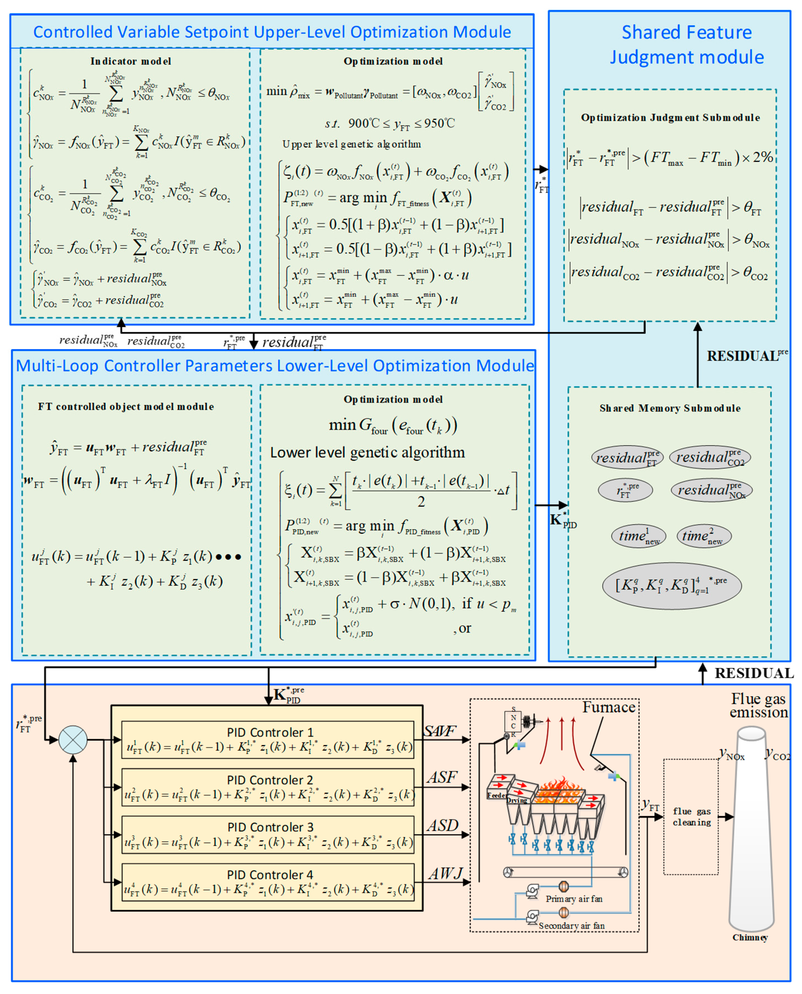
Therefore, the optimal FT setpoint and the optimal multi-loop PID controller parameters are aimed to be obtained in real time by the dual-layer optimization control strategy. The strategy framework consists of an upper-layer optimization module for the controlled variable setpoint, a lower-layer optimization module for multi-loop controller parameters, and a shared memory judgment module, as shown in Figure 2.
In Figure 2, K PID * = [ K P q , K I q , K D q ] q = 1 4 * represents the optimal multi-loop PID controller parameter set vector; r FT * represents the optimal FT setpoint for the minimum pollutant concentration; r FT * , pre represents the historical optimal FT setpoint for the minimum pollutant concentration; R E S I D U A L = [ r e s i d u a l FT ,   r e s i d u a l NOx ,   r e s i d u a l CO 2 ] represents the residual value unitless vector; R E S I D U A L pre = [ r e s i d u a l FT pre ,   r e s i d u a l NOx pre ,   r e s i d u a l CO 2 pre ] represents the historical residual value unitless vector; r e s i d u a l FT represents the FT residual value; r e s i d u a l NOx represents the NOx residual normalized value; r e s i d u a l CO 2 represents the CO2 residual normalized value; r e s i d u a l FT pre represents the historical FT residual value; r e s i d u a l NOx pre represents the historical NOx residual normalized value; r e s i d u a l CO 2 pre represents the historical CO2 residual normalized value; θ FT represents the FT residual value update threshold; θ NOx represents the NOx residual value update threshold; θ CO 2 represents the CO2 residual value update threshold; K PID * , pre = [ K P q , K I q , K D q ] q = 1 4 * , pre represents the historical optimal multi-loop PID controller parameter set vector; γ ^ NO X and γ ^ CO 2 represent the output values of the NOx and CO2 models, respectively; y NOx and y CO 2 represent the actual outputs of NOx and CO2, respectively; y FT represents the actual FT output; y ^ FT represents the output of the FT controlled object model; and S A V F , A S F , A S D and A W J are four key process parameters output by the PID intelligent controller and provided to the actuators: they represent the setpoints for secondary air volumetric flowrate, feeder average speed, dryer average speed, and ammonia injection amount, respectively.
To address the above issues, a dual-layer optimization control strategy is proposed in this article, with the functions of different modules described as follows:
(1)
Controlled Variable Setpoint Upper-Level Optimization Module: The optimal FT setpoint ( r FT * ) that minimizes pollutant concentration is solved using the genetic algorithm (GA), based on the pollutant emission model.
(2)
Multi-Loop Controller Parameters Lower-Level Optimization Module: The optimal multi-loop PID parameters ( [ K P q , K I q , K D q ] q = 1 4 * ) are determined using GA, with r FT * as input and the goal of minimizing ITAE, achieving rapid and precise setpoint tracking.
(3)
Shared Feature Judgment module: Shared memory is used as the parameter transmission medium between the optimization layer and the control layer, and the decision to execute the optimization program again is made based on intermediate parameters.

2.2.1. Controlled Variable Setpoint Upper-Level Optimization Module

In this article, only the combined emission indicators of NOx and CO2 are considered, and the optimization objective is set as the minimization of the weighted emission concentrations of key pollutants (NOx and CO2), so that the environmentally driven optimal FT setpoints can be determined. The model is as follows:
min ρ ^ mix = w Pollutant γ Pollutant = [ ω NOx , ω CO 2 ] γ ^ NOx γ ^ CO 2 s . t . 900   °C y FT 950   °C ω NOx + ω CO 2 = 1 γ ^ NOx = γ ^ NOx + r e s i d u a l NOx pre γ ^ CO 2 = γ ^ CO 2 + r e s i d u a l CO 2 pre
where ρ ^ mix represents the combined emission concentration of NOx and CO2; w Pollutant represents the weight vector of NOx and CO2.; γ Pollutant represents the unitless output vector of the emission concentrations of NOx and CO2; ω NOx represents the weight of the NOx emission concentration; ω CO 2 represents the weight of the CO2 emission concentration; γ ^ NOx represents the compensated NOx model normalized output; γ ^ CO 2 represents the compensated CO2 model normalized output; γ ^ NOx represents the NOx model normalized output; γ ^ CO 2 represents the CO2 model normalized output; r e s i d u a l NOx pre represents the normalized compensation value of the NOx model; and r e s i d u a l CO 2 pre represents the normalized compensation value of the CO2 model.
The transformed single-objective optimization model is solved by GA to obtain the optimal FT setpoint under the condition of minimal pollutant emissions. To ensure the effective implementation of the online dual-layer closed-loop optimization framework, only the standard genetic algorithm improved for MSWI is employed.
The implementation process of GA is composed of population initialization, fitness evaluation, selection, crossover, mutation, and termination condition checking, and is described as follows.
(1).
Initialization of the population
After the parameters of the upper-level genetic algorithm, such as the population size N FT , the maximum number of iterations N FT , iter , the crossover rate c FT , 1 , the mutation rate c FT , 2 , and the upper and lower bounds of the decision variable, are set, the initial population P FT ( 0 ) is generated by a uniform distribution random sampling strategy. As the upper level is a single-variable, single-objective optimization algorithm, only one decision variable (FT) is involved. The mathematical expression for population initialization is given as follows:
x i , FT ( 0 ) = u ( x FT max x FT min ) + x FT min ( i = 1 , 2 , , N FT )
where u represents a random number within the range(0,1); x i , FT ( 0 ) represents the value of the i-th individual gene (FT) of the 0th generation population (initialized population) in the upper-level optimization algorithm; x FT max and x FT min represent the maximum and minimum values of the individual gene (FT), respectively; and N FT represents the population size of the upper-level optimization algorithm.
The distribution of individual genes in the population is shown in Figure 3:
(2).
Fitness function design
The minimization of the weighted concentration of pollutants is set as the optimization objective:
ζ i ( t ) = ρ ^ mix                 = f FT_fitness X i , FT ( t ) = f FT_fitness x i , FT ( t )                 = ω NO x f NO x x i , FT ( t ) + ω CO 2 f CO 2 x i , FT ( t )
f N O x ( x i , FT ( t ) ) = γ ^ NO x ( x i , FT ( t ) ) N O x min N O x max N O x min f C O 2 ( x i , FT ( t ) ) = γ ^ CO 2 ( x i , FT ( t ) ) C O 2 , min C O 2 , max C O 2 , min
where ζ i ( t ) represents the fitness of the i-th individual in the upper-level optimization at the t-th iteration; f FT_fitness represents the FT fitness function in the upper-level optimization algorithm; X i , FT ( t ) represents the D FT -dimensional gene vector of the i-th individual at the t-th iteration, D FT = 1 ; x i , FT ( t ) represents the value of the iii-th individual’s gene (FT) at the t-th iteration; f NOx ( ) and f CO 2 ( ) represent the normalization functions for the NOx and CO2 pollutant indicator models; γ ^ NO x ( ) and γ ^ CO 2 ( ) represent the compensated NOx and CO2 pollutant indicator model functions; N O x max and N O x min represent the maximum and minimum values of NOx emissions; and C O 2 , max , C O 2 , min represent the maximum and minimum values of CO2 emissions.
(3).
Selection operator
A hybrid strategy combining tournament selection and elitist retention is adopted. In the tournament selection strategy, the selection pressure is increased by first randomly selecting k = 3 individuals to form a competition group, then arranging them in ascending order of fitness, and finally allowing the best individual to be chosen for entry into the mating pool.
Then, an elitist retention strategy is incorporated, in which the top two individuals with the highest fitness in each generation are preserved for transfer to the next generation, as expressed by the following formula:
P FT , new ( 1 : 2 ) ( t ) = arg min i     f FT_fitness X i , FT ( t )
where P FT , new ( 1 : 2 ) ( t ) represents the first two individuals in the population of the t-th iteration; and arg min i     f FT_fitness ( ) represents the two individuals that minimize the objective function.
(4).
Crossover Operator
Since the population is encoded in real numbers, each individual contains only one gene value, and therefore simulated binary crossover (SBX) is employed. By utilizing the statistical characteristics of SBX, a balance between global search and local exploitation in the continuous solution space is achieved. The core idea lies in controlling the distribution exponent, by which the probability distribution of the offspring’s distance from their parents is determined, thereby ensuring that diverse individuals are generated without disrupting the structure of high-fitness individuals. Finally, the offspring are rounded to integers and constrained within the maximum and minimum temperature bounds. The crossover operator is formulated as follows:
x i , FT ( t ) = 0.5 [ ( 1 + β ) x i , FT ( t 1 ) + ( 1 β ) x i + 1 , FT ( t 1 ) ] x i + 1 , FT ( t ) = 0.5 [ ( 1 β ) x i , FT ( t 1 ) + ( 1 + β ) x i + 1 , FT ( t 1 ) ]
β = 2 u 1 η + 1                                               if   u 0.5 1 2 ( 1 u ) 1 η + 1                   if   u > 0.5
where u represents a random number within the range (0,1); η represents the distribution index (set to 20); x i , FT ( t 1 ) and x i + 1 , FT ( t 1 ) represent the i-th and (i + 1)-th parent individual FT genes in the upper-level optimization algorithm; and x i , FT ( t ) , x i + 1 , FT ( t ) represent the i-th and (i + 1)-th offspring individual FT genes produced in the upper-level optimization algorithm.
(5).
Mutation Operator
In this article, a hybrid mutation strategy is innovatively employed in the upper-level optimization, by which the search speed is effectively improved while the population is prevented from falling into local optima. The hybrid mutation is defined as a combination of linear decay mutation and uniform mutation. Through linear decay mutation, the convergence toward the optimal solution is accelerated as the number of iterations increases, whereas uniform mutation is applied to maintain global search capability and to prevent the population from being trapped in local optima. During the traversal of population individuals, mutation is triggered probabilistically, leading to two individuals being subjected to mutation, one by linear decay mutation and the other by uniform mutation.
x i , FT ( t ) = x FT min + ( x FT max x FT min ) α u x i + 1 , FT ( t ) = x FT min + ( x FT max x FT min ) u
where α represents the upper-level mutation decay factor; and u represents a random number within the range (0,1).
α = N FT , iter t upper N FT , iter
where N FT , iter represents the maximum number of iterations in the upper-level optimization; and t upper represents the count of optimization generations in the upper-level.

2.2.2. Multi-Loop Controller Parameters Lower-Level Optimization Module

In this lower layer, only the effects of SAVF, ASF, ASD, AWJ, and PAVF (as disturbance variables) on FT are considered. To achieve precise tracking of the target temperature, the Integral of Time-weighted Absolute Error (ITAE) is minimized as the optimization objective, by which the optimal parameters of the multi-loop PID controller are determined. The lower-layer optimization model is presented as follows:
min G four e four ( t k ) = G four r four ( t k ) r four * ( t k )
r four = Θ four u PAVF , u SAVF , u ASF , u ASD , u AWJ + r e s i d u a l FT pre u SAVF , u ASF , u ASD , u AWJ = Φ four r , r * s . t . u SAVF min u SAVF u SAVF max u ASF min u ASF u ASF min u ASD min u ASD u ASD min u AWJ min u AWJ u AWJ max
where G four represents the time-weighted absolute error integral (ITAE) calculation process under the selected manipulated variable; Φ four ( ) represents the PID intelligent controller calculation process under the selected manipulated variable; Θ four represents the controlled object model under the selected manipulated variable; u SAVF , u ASF , u ASD , u AWJ represents the next controller output values for the ASF, ASD, AWJ, and PAVF manipulated variables after PID computation; and r e s i d u a l FT pre represents the FT residual.
The lower-layer single-objective optimization model is solved by GA, so that the optimal parameters of the multi-loop PID controller under the condition of minimal ITAE can be obtained. In this study, only the standard genetic algorithm improved for MSWI control is employed. The specific implementation process of GA is described as follows.
(1).
Initialization of the population
After the parameters of the lower-layer genetic algorithm, such as the population size N PID , number of iterations N PID , iter , crossover rate c PID , 1 , mutation rate c PID , 2 , and the upper and lower bounds of the decision variables, are set, the initial population P PID ( 0 ) is generated by adopting a uniform distribution random sampling strategy. Since the lower layer is formulated as a multi-variable single-objective optimization algorithm, there are D PID = 12 decision variables, which correspond to the four-loop PID parameters K PID = [ K P q , K I q , K D q ] q = 1 4 . The mathematical expression for the population initialization is as follows:
x i , j , PID ( 0 ) = u ( x j , PID max x j , PID min ) + x j , PID min ( i = 1 , 2 , , N PID ; j = 1 , 2 , , D PID )
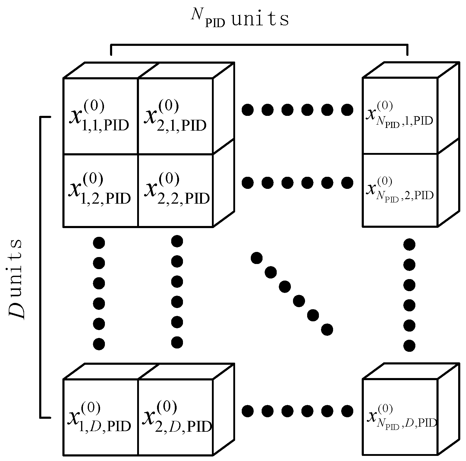
where u represents a random number within the range (0, 1); x i , j , PID ( 0 ) represents the value of the j-th gene (one of the parameters in the 4 PID controllers) of the i-th individual in the 0-th generation population (initialized population) of the lower-level optimization algorithm; x j , PID max and x j , PID min represent the maximum and minimum values of the j-th gene in the lower-level optimization, respectively; N PID represents the population size of the lower-level optimization; and D PID represents the number of individual genes in the lower-level optimization.
The distribution of individual genes in the population is shown in Figure 4:
(2).
Fitness function design
The individual in the population is used as the input to the fitness function, with its gene taken as the parameters of a multi-loop PID controller. The tracking performance of the controller with respect to the optimal FT setpoint is then recorded, and the Integral of Time-weighted Absolute Error (ITAE) is calculated. The minimization of ITAE is adopted as the optimization objective in this study, and the trapezoidal method is employed for the computation of the ITAE. Since ITAE penalizes long-term errors, it is more consistent with the engineering requirement of achieving rapid and stable control.
ξ i ( t ) = G four e four ( t k )                         = f PID_fitness X i , PID ( t )
r four = Θ four u PAVF , u SAVF , u ASF , u ASD , u AWJ + r e s i d u a l FT u SAVF , u ASF , u ASD , u AWJ = Φ four , X i , PID ( t ) r , r *
where ξ i ( t ) represents the fitness of the i-th individual in the lower-level optimization at the t-th iteration; X i , PID ( t ) represents the multi-loop PID controller parameter gene vector of the i-th individual in the t-th generation; and Φ four , X i , PID ( t ) represents the calculation process of the PID intelligent controller using the i-th individual’s parameters in the t-th generation.
(3).
Selection Operator
The selection operator is defined in a manner consistent with the upper-layer method, and the specific formula is presented as follows:
P PID , new ( 1 : 2 ) ( t ) = arg min i   f PID_fitness X i , PID ( t )
where P PID , new ( 1 : 2 ) ( t ) represents the first two individuals in the population at the t-th iteration; and arg min i   f PID_fitness represents the two individuals that minimize the objective function.
(4).
Crossover Operator
A group simulated binary crossover is adopted, in which each PID parameter is treated as an integral unit. For parameter recombination, three parameters of a randomly selected PID controller are employed as a crossover unit, so that the dynamic coupling relationship among PID parameters is preserved. The formula is expressed as follows:
Χ i , k , SBX ( t ) = { x i , 3 k 2 ( t ) , x i , 3 k 1 ( t ) , x i , 3 k ( t ) } ,     k = 1 , , 4
Χ i , k , SBX ( t ) = β Χ i , k , SBX ( t 1 ) + ( 1 β ) Χ i + 1 , k , SBX ( t 1 )             k = 1 , , 4 Χ i + 1 , k , SBX ( t ) = ( 1 β ) Χ i , k , SBX ( t 1 ) + β Χ i + 1 , k , SBX ( t 1 )         k = 1 , , 4
where β ~ Ν ( 1 , 0.5 ) represents the normally distributed disturbance factor; Χ i , k , SBX ( t 1 ) and Χ i + 1 , k , SBX ( t 1 ) represent the k-th gene group of the i-th and (i + 1)-th parent individuals in the lower-level optimization algorithm; and Χ i , k , SBX ( t ) , Χ i + 1 , k , SBX ( t ) represent the k-th gene group of the i-th and (i + 1)-th offspring individuals produced in the lower-level optimization algorithm.
(5).
Mutation Operator
An adaptive Gaussian mutation is employed, in which Gaussian perturbation is combined with boundary reflection (Formula (29)). Compared with traditional uniform mutation, optimization speed can be improved. The formula is expressed as follows:
x i , j , PID ( t ) = x i , j , PID ( t ) + σ N ( 0 , 1 ) ,   if   u < p m x i , j , PID ( t )                                             , or
x i , j , PID ( t ) = 2 x j , PID min x i , j , PID ( t ) ,         if   x i , j , PID ( t ) < x j , PID min 2 x j , PID max x i , j , PID ( t ) ,         else   if   x i , j , PID ( t ) > x j , PID max x i , j , PID ( t ) ,                                         else  
σ = 0.1 + 0.4 u
where σ represents the mutation intensity in the lower-level optimization algorithm, serving as a scaling factor to control the magnitude of the random disturbance; N ( 0 , 1 ) represents the standard normal distribution; u represents a random number within the range (0, 1); x i , j , PID ( t ) represents the gene before mutation in the lower-level optimization; x i , j , PID ( t ) represents the gene after mutation in the lower-level optimization; and x i , j , PID ( t ) represents the gene after boundary reflection when it exceeds the range in the lower-level optimization.

2.2.3. Shared Feature Judgment Module

Shared Memory Submodule
Data are transmitted between the optimization layer and the control layer through shared memory, in a bidirectional manner that allows independent operation without mutual interference.
(1).
Control layer→-ptimization layer: The actual operational FT and pollutant emission concentrations generated by the combustion furnace, together with the corresponding average residuals between the predictive model and the actual measurements, are recorded in real time. The obtained residuals are transmitted back to the optimization module, where the predictive model is updated to adapt to new operating conditions, thereby yielding new optimal variables. The update of residuals is determined by the judgment module: when the difference between the current residuals and the historical residuals exceeds a predefined threshold, the residuals r e s i d u a l CO 2 pre and r e s i d u a l NOx pre are updated.
(2).
Optimization Layer→Control Layer: The optimal FT setpoint r FT and the optimal multi-loop PID parameters K PID * , obtained from the upper- and lower-layer optimization algorithms, are stored and made available for retrieval by the control layer. Through the judgment module, the current r FT is compared with the historical optimal FT setpoint r FT * , p r e . When the threshold is exceeded, r FT * , pre is updated, and the lower-layer optimization algorithm is re-executed. At the same time, a check is performed to determine whether the residual value has been updated; if the residual r e s i d u a l FT pre is updated, the lower-layer optimization algorithm is re-executed again.
Optimization Judgment Submodule
The upper-layer optimization algorithm is executed every 5 min, during which it is determined whether the average residuals between the actual NOx and CO2 outputs and the model outputs exceed the threshold. If the threshold is exceeded, the historical residuals are updated, and the upper-layer optimization algorithm is re-executed.
r e s i d u a l NOx r e s i d u a l NOx pre > θ NOx r e s i d u a l CO 2 r e s i d u a l CO 2 pre > θ CO 2
r e s i d u a l NOx pre = r e s i d u a l NOx r e s i d u a l CO 2 pre = r e s i d u a l CO 2
where r e s i d u a l NOx pre represents the historical average residual value of NOx stored in the shared memory; and r e s i d u a l CO 2 pre represents the historical average residual value of CO2 stored in the shared memory.
The lower-layer optimization algorithm is executed every 30 min, during which it is determined whether the average residual between the actual FT output and the FT model output exceeds the threshold. If the threshold is exceeded, the historical residuals are updated, and the lower-layer optimization algorithm is re-executed.
r e s i d u a l FT r e s i d u a l FT pre > θ FT
r e s i d u a l FT pre = r e s i d u a l FT
where r e s i d u a l FT pre represents the historical average residual value of FT stored in the shared memory.
According to the characteristics of the upper-layer optimization objective, less computational resources are consumed during the upper-layer optimization process, and the optimal solution can be rapidly obtained. In contrast, in the lower-layer optimization, the fitness of each individual is calculated by simulating the PID control process within the fitness function, which results in longer computation times. Therefore, a “lower-layer optimization startup mechanism” is introduced to determine whether the lower-layer optimization should be re-executed. Under this mechanism, when the changes in the upper-layer optimization results fall within a certain range, the lower-layer optimization is not re-executed. The specific formula is as follows.
r FT r FT * , pre > F T max F T min × 2 %
where r FT represents the optimal FT setpoint for the minimum pollutant concentration; r FT * , pre represents the historical optimal FT setpoint for the minimum pollutant concentration stored in the shared memory; and F T max , F T min represent the maximum and minimum values of the optimal FT setpoint, respectively.

2.2.4. Pseudocode

The core execution logic of the dual-layer optimization control strategy proposed in this paper is constituted by three algorithmic modules. In the subsequent subsection, the pseudocode for the upper-layer optimization, lower-layer optimization, and shared-memory judgment algorithms will be elaborated upon, with a focused summary provided for their respective inputs and outputs.
Upper-Level Optimization Algorithm
This algorithm is designed to solve for the optimal FT setpoint that minimizes the comprehensive emission concentration of pollutants (NOx and CO2). Its inputs primarily consist of the fundamental parameters of the Genetic Algorithm and the historical residuals of the pollutant models from the shared memory, which are utilized for dynamic compensation of model predictions. Through the iterative optimization process of the Genetic Algorithm, its output is a specific optimal FT setpoint value, which serves as the control target for the lower-layer tracking control. The specific pseudocode is presented in Algorithm 1.
Algorithm 1: Upper-Level Optimization Algorithm
Input:Population size N FT , maximum iterations N FT , iter , crossover rate c FT , 1 , mutation rate c FT , 2 , model historical residual value r e s i d u a l NOx pre , r e s i d u a l NOx pre ;
Step 1:Initialize the algebraic counter t upper , randomly generate the initial population individual genes according to Formula (12), and finally produce the upper-level initial population P FT ( 0 ) ;
Step 2:Calculate the fitness of the initial population according to Equations (13) and (14);
Step 3:Record the current optimal solution of the population and save it as the global best individual;
Step 4:Iteration begins, while t upper = 1 : N FT , iter ;
Step 5:Use tournament selection to choose parent individuals from the current population;
Step 6:According to Formulas (16) and (17), for the selected parent individuals, simulation two is performed with probability c FT , 1 ;
Step 7:Perform crossover; according to Formulas (18) and (19), for the individuals after crossover, execute the hybrid mutation operation with probability c FT , 2 ;
Step 8:Calculate the fitness of the new population according to Equations (13) and (14);
Step 9:if global optimal individual fitness < new population worst individual fitness;
Step 10:The globally optimal individual replaces and eliminates the worst individual in the new population;
Step 11:end if;
Step 12:If the fitness of the new population’s optimal individual < the fitness of the global optimal individual;
Step 13:Save the best individual in the new population to the global best individual;
Step 14:end if;
Step 15:end while;
Output:The optimal FT setting r FT * .
Lower-Level Optimization Algorithm
This algorithm is responsible for optimizing the parameters of the multi-loop PID controllers to ensure the system can rapidly and accurately track the optimal FT setpoint provided by the upper layer. The inputs encompass the Genetic Algorithm parameters, the historical residual of the FT model, and the historically optimal setpoint obtained from the upper-layer optimization. Utilizing the Integral of Time-weighted Absolute Error (ITAE) as the performance index, the optimization is conducted through improved genetic operations. The final output is an optimal set of parameters for the multi-loop PID controllers. The specific pseudocode is presented in Algorithm 2.
Algorithm 2: Lower-Level Optimization Algorithm
Input:Population size N PID , maximum number of iterations N PID , iter , crossover rate c PID , 1 , mutation rate c PID , 2 , model historical residual value r e s i d u a l FT pre ; the historically optimal r FT * , pre
Step 1:Initialize the algebraic counter t lower , randomly generate the initial population individual genes according to Formula (22), and finally produce the initial lower-level population P PID ( 0 ) ;
Step 2:Calculate the fitness of the initial population according to Equations (23) and (24);
Step 3:Record the current optimal solution of the population and save it as the global best individual;
Step 4:Iteration begins, while t lower = 1 : N PID , iter ;
Step 5:Using tournament selection and elitist selection according to Formula (25), select parent individuals from the current population;
Step 6:According to Formulas (26) and (27), for the selected parent individuals, perform grouping simulation binary crossover with probability c PID , 1 .
Step 7:According to Equations (28) and (29), adaptive Gaussian mutation is performed on the crossed individuals with a probability of c PID , 2 .
Step 8:Calculate the fitness of the new population according to Equations (23) and (24);
Step 9:If optimal individual fitness of the new population< global optimal individual fitness;
Step 10:Save the optimal individual from the new population as the global optimal individual;
Step 11:end if
Step 12:If fitness reaches the threshold
Step 13:break while
Step 14:end if
Step 15:end while
Output:The optimal PID parameter settings value [ K P q , K I q , K D q ] q = 1 4 * for this optimization.
Shared Memory Judgment Algorithm
This algorithm is designed to function as an intelligent coordinator that connects the dual-layer optimization with the real-time control process. Its inputs are derived from the real-time model residuals obtained through actual process monitoring. By comparing these real-time residuals against historical residuals and predefined thresholds, the algorithm determines whether significant changes in process characteristics have occurred. Based on this judgment, a decision is made regarding whether to update the model compensation values and re-trigger either the upper or lower-layer optimization. The outputs consist of the updated historical residuals, historically optimal setpoints, and historically optimal PID parameters. These outputs are written into the shared memory to guide the optimization and control procedures for the subsequent operational cycle, thereby achieving online self-adaptation and closed-loop management of the system. The specific pseudocode implementation is presented in Algorithm 3. A complete list of the main mathematical symbols used in this paper and their meanings is provided in Appendix A (Table A1).
Algorithm 3: Shared Memory Judgment Algorithm
Input:Model residual values r e s i d u a l NOx , r e s i d u a l CO 2 , r e s i d u a l FT ;
Step 1:Initialize shared memory
Step 2:Read residual values, and historical residual values r e s i d u a l NOx pre
r e s i d u a l CO 2 pre from shared memory
Step 3:According to Equation (31), if the condition is met, update r e s i d u a l NOx pre and r e s i d u a l CO 2 pre , and re-execute the upper-layer optimization algorithm to obtain the optimal FT setpoint r FT * ; otherwise, skip.
Step 4:Read the residual value r e s i d u a l FT , the historical residual value r e s i d u a l FT pre , and the historical optimal FT setpoint r FT * , pre from shared memory.
Step 5:Evaluate according to Equations (33) and (35); if the conditions are satisfied, update r e s i d u a l FT pre and r FT * , pre , re-execute the lower-layer optimization algorithm to obtain the optimal multi-loop PID controller parameters [ K P q , K I q , K D q ] q = 1 4 * and update [ K P q , K I q , K D q ] q = 1 4 * , pre ; otherwise, skip;
Step 6:end;
Output:The historical model residuals r e s i d u a l NOx pre , r e s i d u a l CO 2 pre , and r e s i d u a l FT pre ; the historically optimal multi-loop PID controller parameters [ K P q , K I q , K D q ] q = 1 4 * , pre ; and the historically optimal r FT * , pre .

3. Results

3.1. Parameter Settings

The parameters of the genetic algorithm employed in this study are presented in Table 1.
The parameter configuration has been specifically designed for the dual-layer optimization architecture. The upper-layer population size is set to 30 to balance computational efficiency and global exploration, whereas the lower-layer population is set to 50 to enhance diversity and support the fine-tuning of PID parameters. The maximum number of iterations is set to 50 for the upper layer, as the fitness function at this level is less time-consuming, ensuring that the algorithm is not prevented from finding the optimal solution due to insufficient iterations, and 20 for the lower layer to guarantee real-time responsiveness. The crossover probability is set to 0.8 to facilitate information exchange and maintain exploration of the solution space. The mutation probability is set to 0.2 for the upper layer to balance global and local mutation, and 0.1 for the lower layer to emphasize local fine-tuning, thereby ensuring control stability. Overall, the parameter settings reflect a clear division of focus: exploration and adaptability are emphasized in the upper layer, while convergence and stability are emphasized in the lower layer, effectively supporting the collaborative optimization of pollutant minimization and temperature tracking.

3.2. Experimental Results

3.2.1. Upper-Layer GA Optimization Results

To address the multi-objective optimization problem, weighting coefficients are used to combine the NOx and CO2 emission reductions into a single-objective function in the upper-layer optimization algorithm. Specifically, the NOx weight coefficient is set to 0.0788, and the CO2 weight coefficient is set to 0.9212 [29]. These values reflect the relative importance assigned to each pollutant in the optimization process. The maximum and minimum values of NOx emissions were found to be 245.35 mg/m3 and 51.03 mg/m3, respectively, while for CO2 emissions, the maximum and minimum values were 10.18% and 6.45%, respectively, as presented in Table 2. Additionally, the feasible range of FT setpoints, used for optimization, is constrained between 900 °C and 950 °C, as shown in Table 3. This range was determined based on the data used to train the FT model, which was derived from operational data within this temperature range. The model was trained using process data obtained from the MSWI plant, where the FT was consistently maintained between 900 °C and 950 °C during normal operation. As a result, the optimization is limited to this range to ensure the model’s predictions remain accurate and valid within the conditions it was trained on.
To evaluate the robustness and reliability of the proposed optimization algorithm, the upper-layer Genetic Algorithm (GA) was executed independently 30 times under identical parameter configurations. Because the GA inherently involves random initialization and stochastic genetic operations, multiple runs were necessary to eliminate the influence of random seeds and to verify that the convergence performance was not accidental. The average values and variances of runtime, optimal fitness, and the number of generations required to reach the optimal solution are summarized in Table 4. The small variances among these metrics confirm that the algorithm achieved stable convergence and that the optimization results were consistent across different random initializations. This demonstrates that the algorithm possesses strong robustness and repeatability in solving the upper-layer optimization problem.
It is important to note that in all 30 independent runs, the optimization algorithm reached the maximum number of iterations (50) for the upper-layer optimization. This is because the computational cost of the upper-layer Genetic Algorithm (GA) was relatively low, allowing the algorithm to complete the 50 iterations within a reasonable time frame.
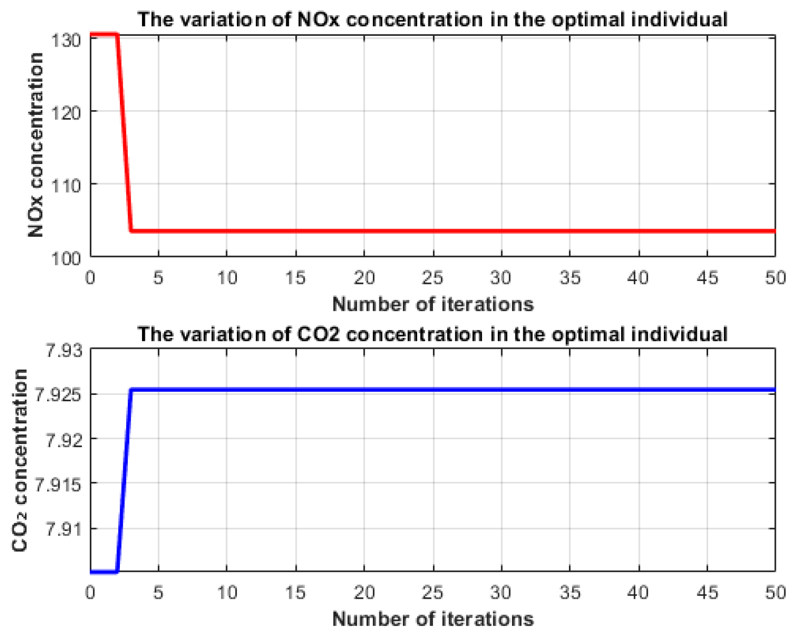
Under the above conditions, the optimal FT setpoint corresponding to the minimum combined pollutant emissions was determined to be 935 °C. A representative single run was selected to illustrate the optimization process. As shown in Figure 5, the fitness curve decreases sharply in the initial iterations and stabilizes after approximately four generations, indicating rapid convergence toward the global optimum. The corresponding variations in pollutant concentrations are shown in Figure 6, where both NOx and CO2 emissions decrease steadily during the optimization process until the minimum point is reached. The smooth and monotonic decline of the curves confirms the effectiveness and convergence stability of the upper-layer GA in minimizing pollutant emissions.
The results obtained from the 30 independent runs demonstrate that the proposed upper-layer Genetic Algorithm (GA) optimization method is both efficient and robust. The runtime data indicate that the algorithm is computationally light, which is crucial for real-time applications, while the optimal fitness values consistently show stable convergence across all runs, further reinforcing the reliability of the algorithm.
The fact that the algorithm always reached the maximum number of iterations (50) does not indicate inefficiency; rather, it reflects the algorithm’s stability. In practice, the algorithm typically finds the optimal FT setpoint within 4 to 6 iterations, which is the range observed during the optimization process. Despite the retention of the 50-generation limit, the algorithm continues to exhibit high efficiency, with each run completing in approximately seconds. This ensures that the optimization process remains computationally efficient and robust, even under the maximum iteration condition. The 50-generation limit is more than sufficient to achieve convergence, while also preventing premature stopping that could affect the optimization results.
In comparison to previous methods, where optimization algorithms have sometimes required more iterations or exhibited higher variability in fitness values, this algorithm proves to be more stable and efficient in achieving the global optimum. However, one potential limitation of the current approach is the dependence on the range of training data. Since the model was trained using operational data within the 900 °C to 950 °C range, its optimization is limited to this range. This means that for operational conditions outside this range, the model’s predictions might become less accurate. Future work could involve extending the training dataset to encompass a broader range of temperatures, improving the model’s ability to generalize and adapt to a wider array of operational conditions.

3.2.2. Lower-Level GA Optimization Results

The lower-layer optimization algorithm is designed to determine the optimal PID parameter settings corresponding to the optimal FT setpoint obtained from the upper-layer optimization. With these optimal PID parameters, the MSWI process can achieve the best convergence of the PID control loops, addressing the challenges associated with manual PID parameter tuning. Moreover, the optimization is performed with respect to the FT setpoint that corresponds to the minimum pollutant concentration, thereby improving the adaptability of the control system to the target temperature.
In this optimization task, the decision variables consist of the four-loop PID parameters for the secondary air volumetric flowrate, feeder, dryer grate, and ammonia injection subsystems. Their allowable ranges were determined based on operational experience and previous research on multi-loop PID tuning for MSWI systems [29]. These parameter ranges define the feasible search space for the GA and are summarized in Table 5, which ensures that each PID parameter remains within a physically meaningful and safe range during the optimization process.
To obtain the optimal PID parameters, the lower-layer GA was executed independently 30 times under identical configurations. The optimization objective was to minimize the Integral of Time-weighted Absolute Error (ITAE), which evaluates both the transient and steady-state performance of the system. The optimized PID parameters obtained under the minimum ITAE condition are presented in Table 6, where each set of parameters represents the optimal control gains for its respective loop. These results ensure that the system achieves fast response, minimal overshoot, and small steady-state error when tracking the optimal FT setpoint.
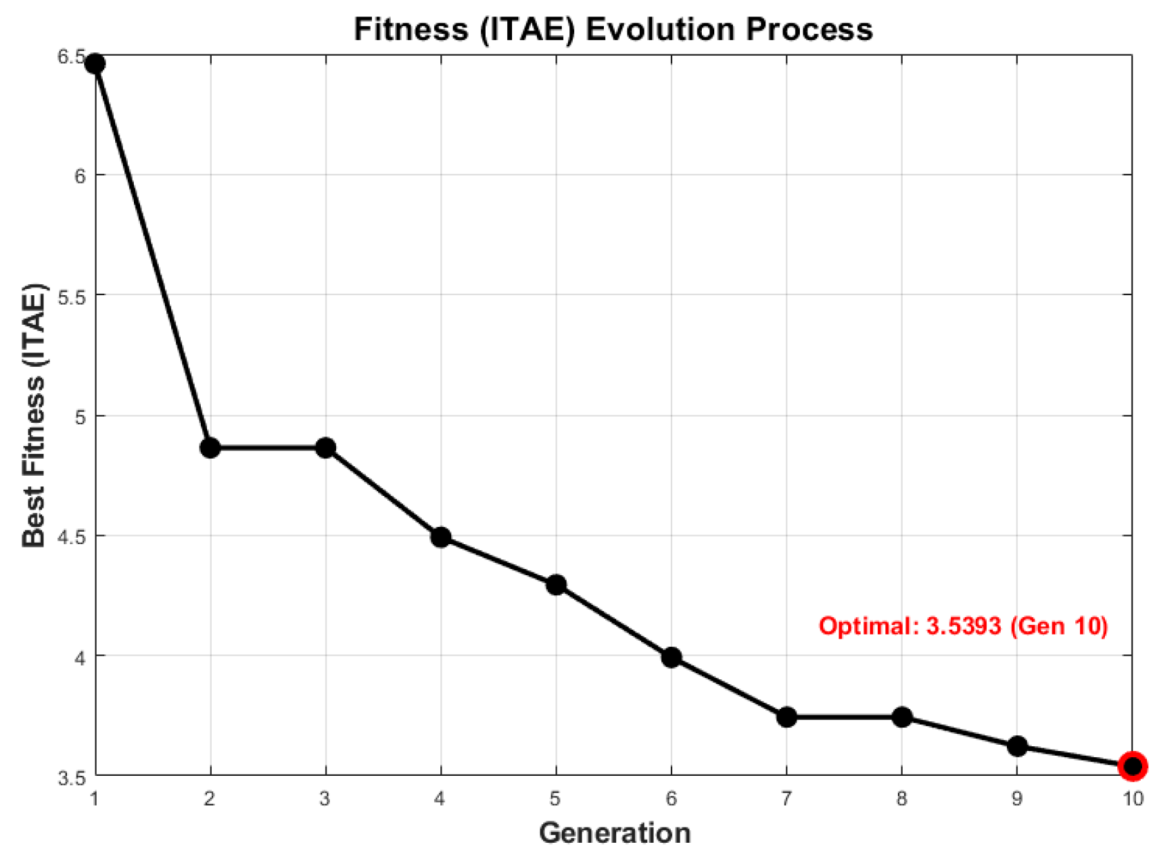
To better understand the optimization process, the convergence behavior of the GA during a representative single run is illustrated in Figure 7. The figure shows how the fitness value decreases rapidly within the first few generations, indicating that the algorithm efficiently identifies promising regions of the search space. After approximately five iterations, the fitness value stabilizes, demonstrating that the algorithm quickly converges to an optimal solution with minimal fluctuation.
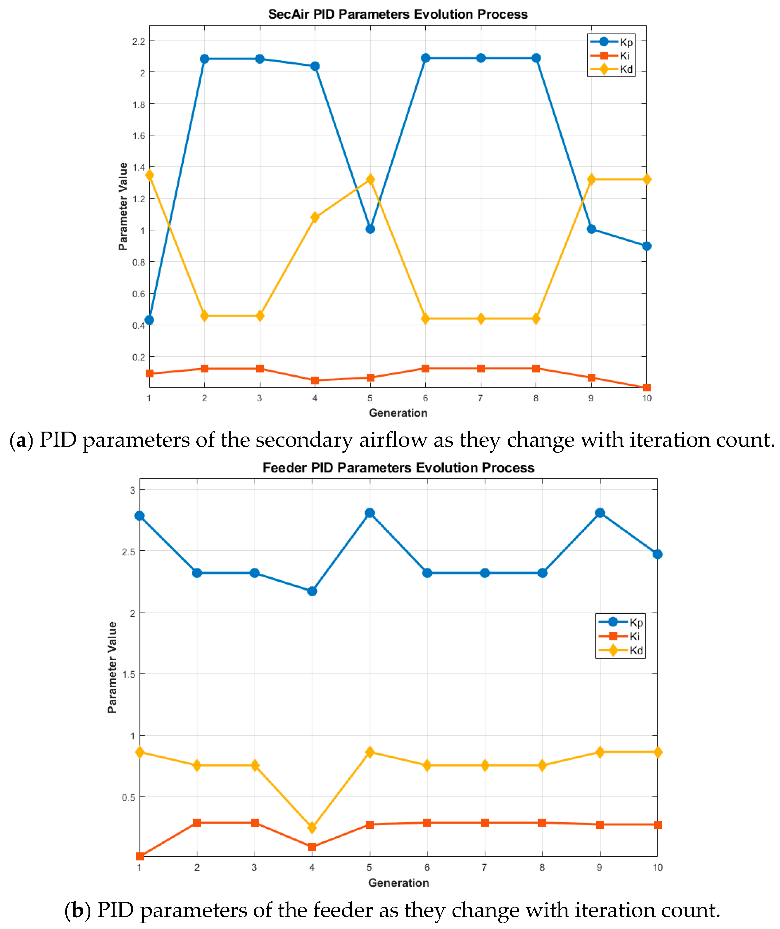
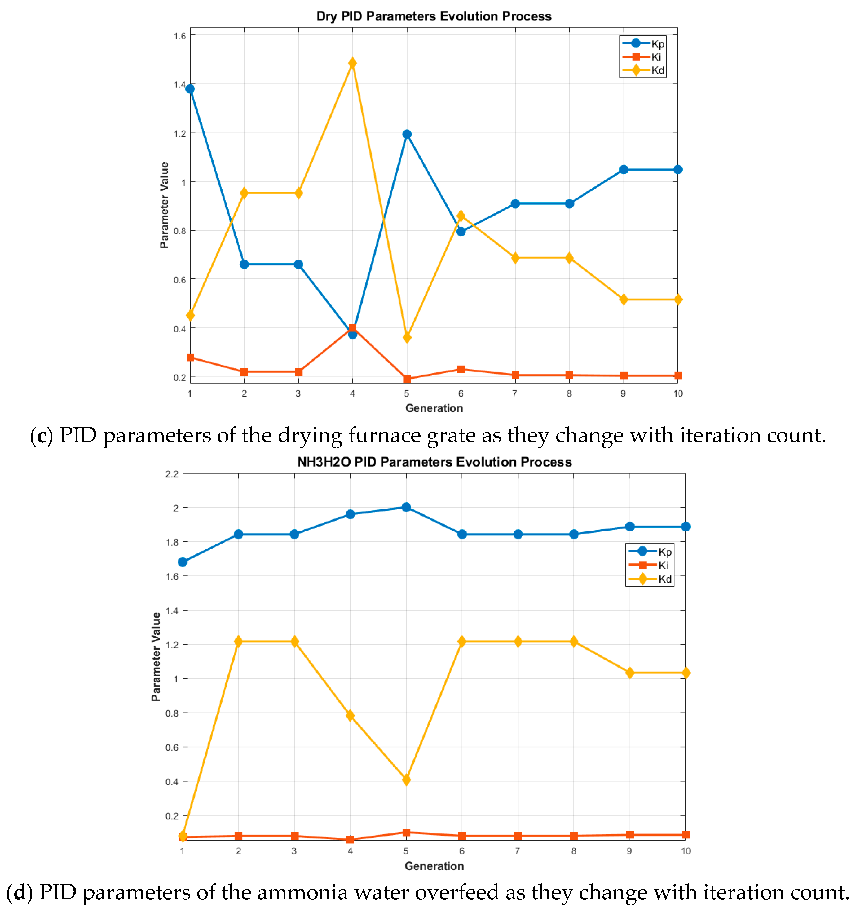
The evolution of the PID parameters for the four control loops throughout the optimization process is shown in Figure 8. Subplots (a)–(d) display the iterative adjustments of each parameter as the GA progresses. It can be observed that each control loop parameter gradually converges to a stable value after several iterations, confirming the algorithm’s capability to fine-tune the PID gains effectively and maintain stability across all loops.
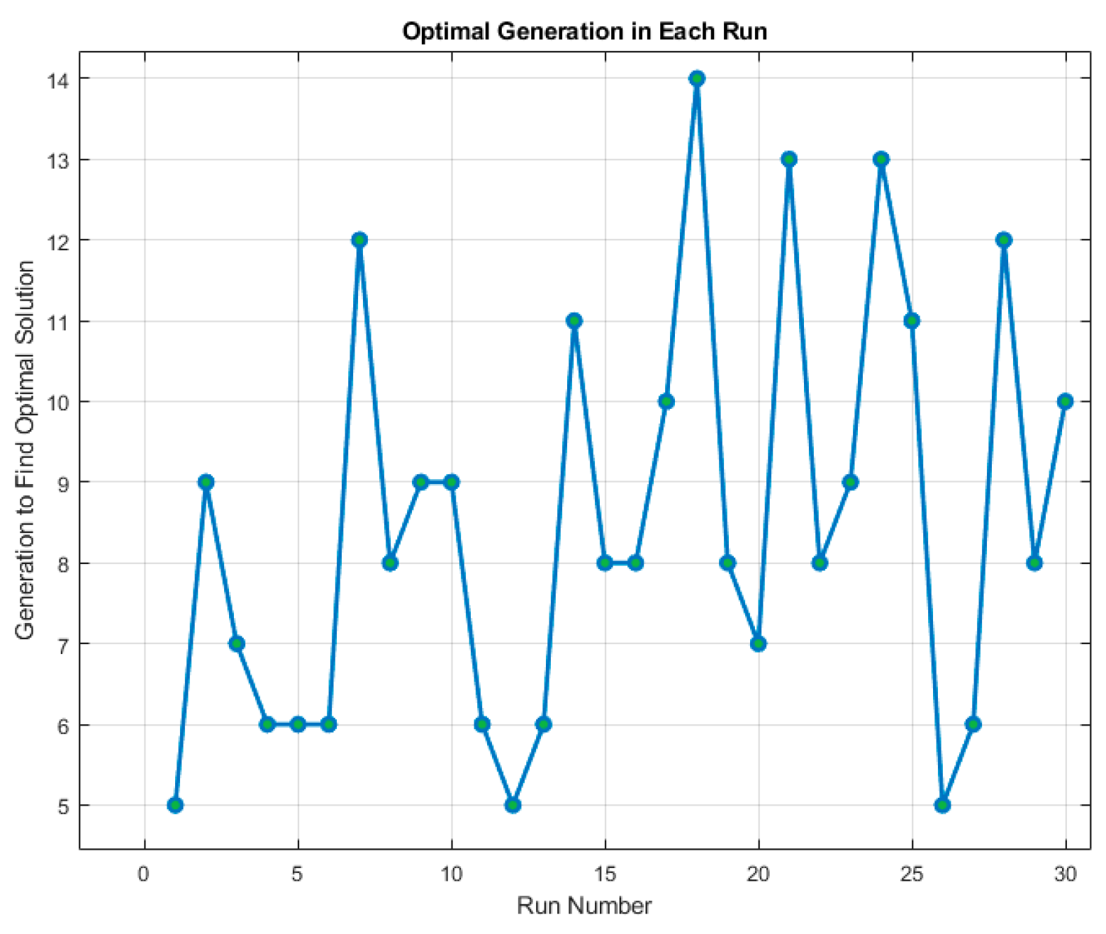
To further illustrate the convergence performance, Figure 9 presents the variation in the number of generations required to reach the optimal solution across 30 independent runs. The figure intuitively shows that the lower-layer GA successfully converged in all runs, and that convergence was always achieved before the maximum iteration limit of 20 generations. This result demonstrates the strong stability and efficiency of the proposed algorithm, indicating that it can reliably locate the optimal solution within a limited number of iterations, regardless of the randomness introduced by different initial populations.
The optimization of the PID controller parameters for the lower-layer optimization algorithm successfully minimizes the Integral of Time-weighted Absolute Error (ITAE), ensuring the optimal control of the FT setpoint. The results indicate that the algorithm efficiently determines the appropriate PID parameters for each loop, which contributes to the stability and effectiveness of the MSWI process.
When comparing the proposed method to traditional manual PID tuning, which often involves trial-and-error adjustments by experts, the optimized algorithm shows clear advantages in terms of accuracy, stability, and computational efficiency. The automated approach eliminates human errors and provides a more reliable and repeatable solution, especially in real-time control scenarios.
One limitation of the current approach is the reliance on the predefined range of PID parameters. Although the algorithm effectively optimizes within the given ranges, it might face difficulties if the system parameters need to be adjusted beyond these ranges due to varying operational conditions or system upgrades. Future research could focus on extending the algorithm to dynamically adjust the PID parameter ranges or incorporate adaptive mechanisms to handle broader and more variable system conditions.

3.2.3. Shared Judgment Results

To enhance the interaction between the upper and lower layers, a shared memory mechanism was introduced to store and exchange residual information between the two optimization layers. The update threshold of this shared memory was determined empirically to balance the feedback frequency and computational stability. The threshold settings used in this study are listed in Table 7, which define the sensitivity of the shared memory updates to residual changes in the optimization process.
(1) The upper-layer GA was executed 30 times with a fixed random seed to eliminate the influence of stochastic initialization and to verify the effect of shared memory feedback under different residual conditions. During each run, random residuals were added to the NOx and CO2 concentrations to simulate fluctuations in system feedback. The residual ranges were set to [−50, 50] for NOx and [−3, 3] for CO2. The purpose of this test was to evaluate whether the shared memory mechanism could effectively handle feedback disturbances and maintain stable optimization performance. The statistical results, including the average and variance of the 30 runs, are presented in Table 8.
(2) In the lower-layer optimization, the GA determines the optimal multi-loop PID parameters corresponding to the compensated FT setpoint. Because this layer involves 12 decision variables, random initialization may cause minor variations in the resulting optimal parameters even under identical termination conditions. To analyze the influence of different residual values on the lower-layer optimization, three control experiments were conducted under a fixed random seed. The residual values were set to −5, 0, and 5, respectively, representing under-compensation, nominal condition, and over-compensation scenarios. The resulting optimal fitness values for these three experiments are summarized in Table 9.
The detailed PID parameters obtained under each residual condition are listed in Table 10, Table 11 and Table 12. These results illustrate the parameter variations among the four control loops under different residual compensation settings.
Although the optimal fitness values obtained for different residual conditions were close in magnitude (Table 9), noticeable variations are observed in the individual PID parameters (Table 10, Table 11 and Table 12). These differences indicate that residual compensation slightly influences the tuning of each loop, especially for the AWJ and ASF controllers, which are more sensitive to system nonlinearities. Nevertheless, the overall optimization results remain stable, confirming that the lower-layer GA maintains consistent convergence behavior under varying residual conditions.

3.3. Method Comparison

3.3.1. PID Performance Perspective

The effectiveness of the proposed dual-layer optimization framework was verified by comparing the PID controller with parameters optimized by the algorithm against both a manually tuned PID controller and an intelligent control method based on an Improved single neuron adaptive PID (ISNA-PID). This comprehensive comparison was designed to evaluate the performance improvements achieved by the proposed automatic optimization strategy over both traditional manual tuning and another contemporary intelligent method. For the manually tuned PID controller, the proportional, integral, and derivative coefficients were empirically set to 0.1, 0.001, and 0.001, respectively. For the ISNA-PID controller, the neural gain coefficient was configured as 0.04, and the learning rates for the proportional, derivative, and integral neurons were set to 0.3, 0.1, and 0.2, respectively. Figure 10 depicts the resulting FT control curves, illustrating the dynamic responses of each controller against the desired setpoint across the sampling instances.
To quantitatively evaluate the tracking performance of different control algorithms in response to changes in the FT setpoint, tests were conducted on three controllers (GA_PID, ISNA_PID, PID) across seven distinct temperature stages. As presented in Table 13, ITAE values were recorded during the process of the system reaching a new steady state after each temperature step change. In addition, to conduct a more comprehensive performance evaluation, the statistical results of ISE, IAE, and DEVmax for the three control algorithms are also listed in Table 14, facilitating a multi-dimensional comparative analysis of the controllers’ performance.
The data in Table 13 clearly demonstrate that the ITAE values of the Genetic Algorithm-optimized controller (GA_PID) are significantly lower than those of both the ISNA_PID and traditional PID controllers across the various temperature stages. This quantitative finding is mutually corroborated by the trend observed in the control curves shown in Figure 10, offering visual proof that the GA_PID achieves faster response speed, reduced overshoot, and superior steady-state accuracy in setpoint tracking. Furthermore, this comparative analysis of the stage-wise ITAE metrics provides compelling data support for the superiority of the proposed dual-layer optimization control strategy in enhancing FT tracking performance.
A detailed analysis of the performance metrics presented in Table 14 reveals that the GA_PID controller demonstrates significantly lower values in both ISE and IAE metrics compared to the ISNA_PID and traditional PID controllers. The lower ISE value indicates that the GA_PID controller is more effective in suppressing large errors during the control process, while the smaller IAE value reflects its superior overall control error level. Although DEVmax was identical for all three controllers in this particular test, the superior performance in ISE and IAE underscores the comprehensive advantage of the GA_PID controller in terms of both response speed and steady-state accuracy.
These quantitative indicators are mutually corroborated by the control curve trends illustrated in Figure 10 and the stage-wise ITAE values listed in Table 13. Collectively, this evidence substantiates the effectiveness of the proposed dual-layer optimization control strategy in enhancing the FT tracking performance.

3.3.2. Pollutant Emissions Perspective

Regarding the search for the global optimal setpoint of FT that minimizes the comprehensive pollutant emission concentration, a comparison is conducted using the GA and PSO algorithm. The experiments are carried out on a PC using Matlab 2020b, with a clock speed of 4.20 GHz and 32 GB RAM, under the Microsoft Windows 10 environment. Both algorithms were configured with identical parameters for a direct comparison: a population size of 30 and a maximum of 50 iterations. Furthermore, the optimization was based on the same set of weighting coefficients for the pollutant concentrations, as defined in the upper-layer optimization model.
The algorithms were independently executed 30 times. The average results from these runs are summarized as follows. The optimal FT setpoint value is 935 °C, and the emission concentration of NOx and CO2 is 103.59 mg/m3N and 7.9255%, respectively. Notably, the variance for these results was zero, indicating exceptionally stable and consistent convergence performance across all runs for both algorithms.
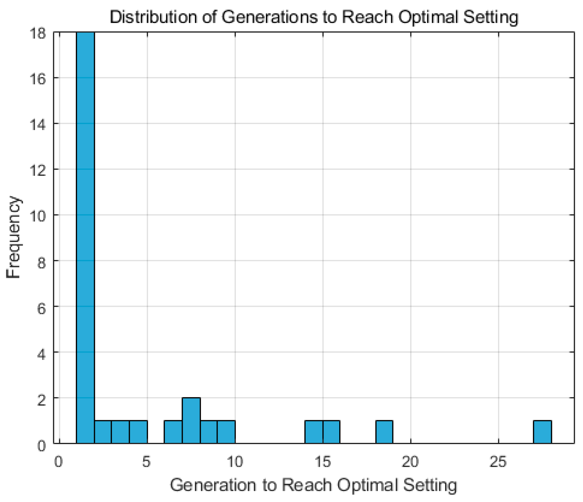
Although identical optimization outcomes were achieved by both the GA and PSO in terms of FT setpoint and pollutant emission minimization, significant disparities were observed in their computational performance metrics. A detailed comparative analysis is systematically presented in Table 15. Moreover, the distribution frequency of the generations required to reach the optimal FT setpoint over 30 independent runs is clearly visualized in Figure 11 and Figure 12.
Although GA and PSO achieved exactly the same optimal FT setpoint and identical pollutant-minimization results, their convergence characteristics exhibited notable differences. GA demonstrated a significantly faster computation speed but showed larger fluctuations in the number of generations required to reach the optimum. In contrast, PSO achieved the optimum with fewer generations and exhibited smaller variance, but its computation time was consistently longer. These findings indicate that GA provides higher computational efficiency, whereas PSO offers more stable convergence behavior.
It should be noted that the operating conditions used in this study were relatively stable and involved a single FT setpoint. When the operating environment becomes more complex such as including multiple setpoints or multiple controlled variables such as FT, steam flow rate, and flue-gas oxygen concentration, the optimization problem will become significantly more challenging. In such cases, the dual-layer optimization framework proposed in this study is expected to exhibit greater efficiency and adaptability.
Future research will consider multi-setpoint and multi-variable scenarios, integrating more complex optimization objectives and constraints, so that the dual-layer structure can further improve environmental performance, control stability, and overall system intelligence under broader MSWI operating conditions.

4. Conclusions

The MSWI process involves complex physical and chemical reactions and operates as a multi-input, multi-output system with multiple loops, strong coupling, and nonlinear characteristics. Consequently, it presents challenges for control experts attempting to minimize pollutant emission concentrations. To address this, a dual-layer optimization control strategy is proposed, which aims to minimize pollutant emissions in accordance with national discharge standards. The contributions of this article are as follows: (1) A dual-layer optimization control method is proposed using an improved genetic algorithm, enabling rapid determination of the optimal FT setpoint and PID controller parameters; (2) A shared memory module is introduced to link the optimization and control layers, achieving closed-loop optimization and overcoming the limitation that offline optimization cannot adapt to real operating conditions; (3) Optimization execution judgment conditions are incorporated to prevent repeated execution under identical constraints, thereby improving optimization efficiency.
However, the FT-controlled object model and the pollutant emission indicator model in this study are constructed only under steady-state operating conditions, and only NOx and CO2 are considered to evaluate the minimum pollutant emission concentrations. In the future, additional pollutant indicators will be incorporated into the bi-level optimization control framework, while economic, energy, and maintenance indicators will also be taken into account to achieve comprehensive optimization. Furthermore, the development of more advanced intelligent optimization algorithms for the MSWI process will be considered to further enhance operational optimization.

Author Contributions

Conceptualization, W.W.; Methodology, W.W. and J.T.; Software, Y.W. and J.R.; Validation, J.R.; Investigation, Y.W.; Resources, Y.W., Z.L. and J.R.; Data curation, Y.W.; Writing—original draft, Y.W.; Writing—review & editing, W.W. and J.T.; Visualization, Y.W. and Z.L.; Supervision, W.W. and J.T.; Project administration, W.W. All authors have read and agreed to the published version of the manuscript.

Funding

This work was supported in part by the General Scientific Research Projects of Liaoning Province Science and Technology Joint Plan Project under Grant 2024JH2/102600083, and in part by Liaoning Provincial Department of Education under Grant JYTMS20230489.

Institutional Review Board Statement

Not applicable.

Informed Consent Statement

Not applicable.

Data Availability Statement

The data presented in this study are available on request from the corresponding author.

Conflicts of Interest

The authors declare no conflict of interest.

Abbreviations

The following abbreviations are used in this manuscript:
MSWMunicipal solid waste
MSWIMunicipal solid waste incineration
FTFT
ITAEIntegral of Time-weighted Absolute Error
GAGenetic algorithm
IMOPSOImproved multi-objective particle swarm optimization
ALMOCSOAdaptive large-scale multi-objective competitive swarm optimization algorithm
PIDProportional-Integral-Derivative
3T+ETemperature, Turbulence, Time, and Excess Oxygen
PAVFPrimary air volumetric flowrate
SAVFSecondary air volumetric flowrate
ASFAverage speed of the feeder grate
ASDAverage speed of the drying grate
AWJAmmonia water injection
SNCRSelective Non-Catalytic Reduction
TR-LRDTTikhonov regularization-least regression decision tree
CARTClassification and regression tree
SBXSimulated binary crossover

Appendix A

Table A1. Symbols used in this article and their meanings.
NumSymbolActual Meaning
1. F Objective function vector
2. F l The l-th indicator model
3. h i Equality constraint
4. g j Inequality constraint
5. x Decision variable vector
6. γ ^ Pollutant emission concentration unitless vector
7. γ ^ n The n-th pollutant model normalized output
8. ρ ^ The combined pollutant emission concentration
9. w Weight vector
10. γ ^ Compensated pollutant emission concentration output unitless vector
11. ω n Weight of the emission concentration of the n-th pollutant
12. γ ^ n Compensated emission model normalized output of the n-th pollutant
13. r e s i d u a l n Normalized compensation value of the n-th pollutant model
14. r FT * Optimal FT setpoint for minimum pollutant concentration
15. r FT * , pre Historical optimal FT setpoint for minimum pollutant concentration
16. G · Trapezoidal method discrete time-weighted absolute error integral function
17. N ITAE Total step length of ITAE
18. Φ · PID intelligent controller calculation process
19. t k Time variable in the PID controller computation process
20. Δ t Time step
21. Θ · FT controlled object model
22. u q The controller output value at the next time step after the PID computation of the q-th manipulated variable
23. K PID * Optimal multivariable PID controller setpoint parameter vector
24. [ K P q , K I q , K D q ] q = 1 4 * Optimal multivariable PID parameters
25. R E S I D U A L Residual value unitless vector
26. R E S I D U A L pre Historical residual value unitless vector
27. r e s i d u a l FT FT residual value
28. r e s i d u a l NOx NOx residual normalized value
29. r e s i d u a l CO 2 CO2 residual normalized value
30. r e s i d u a l FT pre Historical FT residual value
31. r e s i d u a l NOx pre Historical NOx residual normalized value
32. r e s i d u a l CO 2 pre Historical CO2 residual normalized value
33. θ FT FT residual value update threshold
34. θ NOx NOx residual value update threshold
35. θ CO 2 CO2 residual value update threshold
36. y NOx Actual output value of NOx
37. y CO 2 Actual output value of CO2
38. y FT Actual output value of the FT
39. y ^ FT Output value of the FT controlled object model
40. S A V F Setpoint value of the secondary air volumetric flowrate rate output to the actuator after PID intelligent controller computation
41. A S F Setpoint value of the feeder output to the actuator after PID intelligent controller computation
42. A S D Setpoint value of the dryer flow rate output to the actuator after PID intelligent controller computation
43. A W J Setpoint value of the ammonia water injection amount output to the actuator after PID intelligent controller computation
44. ρ ^ mix Comprehensive emission concentration of NOx and CO2
45. w Pollutant Weight vector of NOx and CO2
46. γ Pollutant Output vector of the emission concentrations of NOx and CO2
47. ω NOx Weight of NOx emission concentration
48. ω CO 2 Weight of CO2 emission concentration
49. γ ^ NOx Compensated normalized output of the NOx model
50. γ ^ CO 2 Compensated normalized output of the CO2 model
51. γ ^ NOx Normalized output of the NOx model
52. γ ^ CO 2 Normalized output of the CO2 model
53. x i , FT ( 0 ) Value of the i-th individual gene (FT) in the 0th generation population (initial population) of the upper-level optimization algorithm
54. x FT max Maximum value of the individual gene (FT)
55. x FT min Minimum value of the individual gene (FT)
56. N FT Population size of the upper-level optimization algorithm
57. ζ i ( t ) Fitness of the i-th individual in the upper-level optimization algorithm at the t-th iteration
58. f FT_fitness FT fitness function in the upper-level optimization algorithm
59. X i , FT ( t ) The D FT -dimensional gene vector of the i-th individual at the t-th iteration, where D FT = 1
60. x i , FT ( t ) The value of the gene (FT) of the i-th individual at the t-th iteration
61. f NOx ( ) Normalization function of the NOx pollutant index model
62. f CO 2 ( ) Normalization function of the CO2 pollutant index model
63. γ ^ NO x ( ) Compensated NOx pollutant index model function
64. γ ^ CO 2 ( ) Compensated CO2 pollutant index model function
65. N O x max Maximum value of NOx emissions
66. N O x min Minimum value of NOx emissions
67. C O 2 , max Maximum value of CO2emissions
68. C O 2 , min Minimum value of CO2 emissions
69. P FT , new ( 1 : 2 ) ( t ) The first two individuals in the population at the t-th iteration
70. arg min i f FT_fitness ( ) The two individuals that minimize the objective function
71. x i , FT ( t 1 ) FT gene of the i-th individual in the parent generation of the upper-level optimization algorithm
72. x i + 1 , FT ( t 1 ) FT gene of the (i + 1)-th individual in the parent generation of the upper-level optimization algorithm
73. x i , FT ( t ) FT gene of the i-th individual in the offspring generated by the upper-level optimization algorithm
74. x i + 1 , FT ( t ) FT gene of the (i + 1)-th individual in the offspring generated by the upper-level optimization algorithm
75. α Upper-level mutation decay factor
76. u Random number in the range (0, 1)
77. N FT , iter Maximum number of iterations in the upper-level optimization
78. t upper Upper-level optimization generation count
79. G four Time-weighted absolute error integral (ITAE) calculation process under the selected manipulated variable
80. Φ four ( ) Calculation process of the PID intelligent controller under the selected manipulated variable
81. Θ four · Controlled object model under the selected manipulated variable
82. u SAVF , u ASF , u ASD , u AWJ Represents the next-time-step controller output values of the ASF, ASD, AWJ, and PAVF manipulated variables after PID calculation
83. x i , j , PID ( 0 ) Value of the j-th gene (one of the parameters in the 4 PID controllers) of the i-th individual in the 0-th generation population (initial population) of the lower-level optimization algorithm
84. x j , PID max Maximum value of the j-th gene of an individual in the lower-level optimization
85. x j , PID min Minimum value of the j-th gene of an individual in the lower-level optimization
86. N PID Population size of the lower-level optimization
87. D PID Number of genes per individual in the lower-level optimization
88. ξ i ( t ) Fitness of the i-th individual in the t-th iteration of the lower-level optimization
89. X i , PID ( t ) Multi-loop PID controller parameter gene vector of the i-th individual in the t-th generation
90. Φ four , X i , PID ( t ) Calculation process using the PID intelligent controller of the i-th individual in the t-th generation
91. P PID , new ( 1 : 2 ) ( t ) The first two individuals in the population of the t-th iteration
92. arg min i   f PID_fitness The two individuals that minimize the objective function
93. β   ~   Ν ( 1 , 0.5 ) Gaussian distribution disturbance factor
94. Χ i , k , SBX ( t 1 ) The k-th genome of the i-th individual in the parent generation of the lower-level optimization algorithm
95. Χ i + 1 , k , SBX ( t 1 ) The k-th genome of the (i + 1)-th individual in the parent generation of the lower-level optimization algorithm
96. Χ i , k , SBX ( t ) The k-th genome of the i-th individual in the offspring generation produced by the lower-level optimization algorithm
97. Χ i + 1 , k , SBX ( t ) The k-th genome of the (i + 1)-th individual in the offspring generation produced by the lower-level optimization algorithm
98. σ Mutation strength in the lower-level optimization algorithm, used as a scaling factor to control the magnitude of the random disturbance
99. N ( 0 , 1 ) Standard normal distribution
100. x i , j , PID ( t ) Gene before mutation in the lower-level optimization
101. x i , j , PID ( t ) Gene after mutation in the lower-level optimization
102. x i , j , PID ( t ) Gene after boundary reflection when it exceeds the range in the lower-level optimization
103. F T max The maximum value of the optimal FT setpoint
104. F T min The minimum value of the optimal FT setpoint
105. e ( t k ) The error at step t k
106. e ( t k 1 ) The error at step t k 1

References

  1. Tang, J.; Xia, H.; Yu, F.; Qiao, J. Research Status and Prospects of Intelligent Optimization Control for Municipal Solid Waste Incineration Process. Acta Autom. Sin. 2023, 49, 2019–2059. [Google Scholar] [CrossRef]
  2. Gómez-Sanabria, A.; Kiesewetter, G.; Klimont, Z.; Schoepp, W.; Haberl, H. Potential for Future Reductions of Global GHG and Air Pollutants from Circular Waste Management Systems. Nat. Commun. 2022, 13, 106. [Google Scholar] [CrossRef] [PubMed]
  3. Chen, A.; Chen, J.; Cui, J.; Fan, C.; Han, W. The study on the “Risk of Garbage Surrounding Cities” in 31 Municipalities and Provincial Capitals of China and Countermeasures—An Empirical Study Based on the DIIS Method. Bull. Chin. Acad. Sci. 2019, 34, 797–806. [Google Scholar] [CrossRef]
  4. Vilardi, G.; Verdone, N. Exergy Analysis of Municipal Solid Waste Incineration Processes: The Use of O2-Enriched Air and the Oxy-Combustion Process. Energy 2022, 239, 122147. [Google Scholar] [CrossRef]
  5. Bajić, B.Ž.; Dodić, S.N.; Vučurović, D.G.; Dodić, J.M.; Grahovac, J.A. Waste-to-Energy Status in Serbia. Renew. Sustain. Energy Rev. 2015, 50, 1437–1444. [Google Scholar] [CrossRef]
  6. Walser, T.; Limbach, L.K.; Brogioli, R.; Erismann, E.; Flamigni, L.; Hattendorf, B.; Juchli, M.; Krumeich, F.; Ludwig, C.; Prikopsky, K.; et al. Persistence of Engineered Nanoparticles in a Municipal Solid-Waste Incineration Plant. Nat. Nanotechnol. 2012, 7, 520–524. [Google Scholar] [CrossRef]
  7. Chen, B.; Perumal, P.; Aghabeyk, F.; Adediran, A.; Illikainen, M.; Ye, G. Advances in Using Municipal Solid Waste Incineration (MSWI) Bottom Ash as Precursor for Alkali-Activated Materials: A Critical Review. Resour. Conserv. Recycl. 2024, 204, 107516. [Google Scholar] [CrossRef]
  8. Yang, D.; Kow, K.-W.; Wang, W.; Meredith, W.; Zhang, G.; Mao, Y.; Xu, M. Co-Treatment of Municipal Solid Waste Incineration Fly Ash and Alumina-/Silica-Containing Waste: A Critical Review. J. Hazard. Mater. 2024, 479, 135677. [Google Scholar] [CrossRef]
  9. Kammen, D.M.; Sunter, D.A. City-Integrated Renewable Energy for Urban Sustainability. Science 2016, 325, 922–928. [Google Scholar] [CrossRef]
  10. Kumar, A.; Samadder, S.R. A Review on Technological Options of Waste to Energy for Effective Management of Municipal Solid Waste. Waste Manag. 2017, 69, 407–422. [Google Scholar] [CrossRef]
  11. Long, J.; Du, H.; Zou, X.; Huang, J. A Systematic Study on Carbon Emission Reduction in Urban Household Waste Management. Bull. Chin. Acad. Sci. 2022, 37, 1143–1153. [Google Scholar] [CrossRef]
  12. Liu, Y.; Sun, W.; Liu, J. Greenhouse Gas Emissions from Different Municipal Solid Waste Management Scenarios in China: Based on Carbon and Energy Flow Analysis. Waste Manag. 2017, 68, 653–661. [Google Scholar] [CrossRef]
  13. Asri, R.; Baxter, D. Process Control in Municipal Solid Waste Incinerators: Survey and Assessment. Waste Manag. Res. 2004, 22, 177–185. [Google Scholar] [CrossRef] [PubMed]
  14. Khandelwal, H.; Dhar, H.; Thalla, A.K.; Kumar, S. Application of Life Cycle Assessment in Municipal Solid Waste Management: A Worldwide Critical Review. J. Clean. Prod. 2019, 209, 630–654. [Google Scholar] [CrossRef]
  15. Yu, T.; Ding, H.; Qiao, J. Ensemble Self-Organizing Recursive Neural Network for Modeling Furnace Temperature in Municipal Solid Waste Incineration. Appl. Soft Comput. 2025, 178, 113170. [Google Scholar] [CrossRef]
  16. Wang, J.; Nketiah, E.; Cai, X.; Obuobi, B.; Adu-Gyamfi, G.; Adjei, M. What Establishes Citizens’ Household Intention and Behavior Regarding Municipal Solid Waste Separation? A Case Study in Jiangsu Province. J. Clean. Prod. 2023, 423, 138642. [Google Scholar] [CrossRef]
  17. Lu, M.; Xia, Y.; Yan, J.; Wang, L. Wet Carbonation of MSWI Fly Ash for Sustainable Limestone Calcined Clay Cement-Type Composites. Cem. Concr. Compos. 2025, 156, 105866. [Google Scholar] [CrossRef]
  18. Zhou, H.; Wei, L.; Wang, D.; Zhang, W. Environmental Impacts and Optimizing Strategies of Municipal Sludge Treatment and Disposal Routes in China Based on Life Cycle Analysis. Environ. Int. 2022, 166, 107378. [Google Scholar] [CrossRef]
  19. Hunsinger, H.; Jay, K.; Vehlow, J. Formation and Destruction of PCDD/F inside a Grate Furnace. Chemosphere 2002, 46, 1263–1272. [Google Scholar] [CrossRef]
  20. Yao, X.; Jiao, F.; Gao, S.; Hu, Y.; Liu, T.; Zhang, Y.; Mao, L.; Wu, C.; Li, H.; Dong, Z. Co-Melting Mechanisms for Municipal Solid Waste Incineration Fly Ash with Fine Slag from Coal Gasification and Coal Gangue. J. Environ. Manag. 2024, 367, 122035. [Google Scholar] [CrossRef]
  21. Kolekar, K.A.; Hazra, T.; Chakrabarty, S.N. A Review on Prediction of Municipal Solid Waste Generation Models. Procedia Environ. Sci. 2016, 35, 238–244. [Google Scholar] [CrossRef]
  22. Qiao, J.; Sun, Z.; Meng, X. A Comprehensively Improved Interval Type-2 Fuzzy Neural Network for NOx Emissions Prediction in MSWI Process. IEEE Trans. Ind. Inform. 2023, 19, 11286–11297. [Google Scholar] [CrossRef]
  23. Tang, J.; Wang, T.; Xia, H.; Cui, C. An Overview of Artificial Intelligence Application for Optimal Control of Municipal Solid Waste Incineration Process. Sustainability 2024, 16, 2042. [Google Scholar] [CrossRef]
  24. Wang, T.; Tang, J.; Xia, H.; Yang, C.; Yu, W.; Qiao, J. Data-Driven Multi-Objective Intelligent Optimal Control of Municipal Solid Waste Incineration Process. Eng. Appl. Artif. Intell. 2024, 137, 109157. [Google Scholar] [CrossRef]
  25. Huang, W.; Ding, H.; Qiao, J. Large-Scale and Knowledge-Based Dynamic Multiobjective Optimization for MSWI Process Using Adaptive Competitive Swarm Optimization. IEEE Trans. Syst. Man Cybern. Syst. 2024, 54, 379–390. [Google Scholar] [CrossRef]
  26. Qiao, J.; Cui, Y.; Meng, X. Dynamic Multi-Objective Operation Optimization of Municipal Solid Waste Incineration Process Based on Transfer Learning. IEEE Trans. Autom. Sci. Eng. 2025, 22, 9338–9352. [Google Scholar] [CrossRef]
  27. Samad, T.; Bauer, M.; Bortoff, S.; Di Cairano, S.; Fagiano, L.; Odgaard, P.F.; Rhinehart, R.R.; Sánchez-Peña, R.; Serbezov, A.; Ankersen, F.; et al. Industry Engagement with Control Research: Perspective and Messages. Annu. Rev. Control 2020, 49, 1–14. [Google Scholar] [CrossRef]
  28. Cui, Y.; Meng, X.; Qiao, J. Multi-Condition Operational Optimization with Adaptive Knowledge Transfer for Municipal Solid Waste Incineration Process. Expert Syst. Appl. 2024, 238, 121783. [Google Scholar] [CrossRef]
  29. Wang, T.; Tang, J.; Xia, H.; Aljerf, L.; Zhang, R.; Tian, H.; Akele, M.L. Intelligent Optimal Control of FT for the Municipal Solid Waste Incineration Process Using Multi-Loop Controller and Particle Swarm Optimization. Expert Syst. Appl. 2024, 257, 125015. [Google Scholar] [CrossRef]
  30. Tao, J.; Li, Z.; Chen, C.; Liang, R.; Wu, S.; Lin, F.; Cheng, Z.; Yan, B.; Chen, G. Intelligent Technologies Powering Clean Incineration of Municipal Solid Waste: A System Review. Sci. Total Environ. 2024, 935, 173082. [Google Scholar] [CrossRef]
  31. Tian, H.; Tang, J.; Aljerf, L.; Wang, T.; Qiao, J. FT Control Based on Interval Type-2 Fuzzy Broad Learning System for Municipal Solid Waste Incineration Process. Expert Syst. Appl. 2025, 280, 127530. [Google Scholar] [CrossRef]
  32. Li, Z.; Yao, S.; Chen, D.; Li, L.; Lu, Z.; Yu, Z. Modelling Nitrogen Oxide Emission Trends from the Municipal Solid Waste Incineration Process Using an Adaptive Bi-Directional Long and Short-Term Memory Network. Can. J. Chem. Eng. 2024, 102, 1225–1237. [Google Scholar] [CrossRef]
  33. Sanoj, K.P.; Dhanya Ram, V. Optimal PID Controller Tuning for Multivariable Unstable Systems by Minimizing ITAE Criteria. IFAC Pap. 2024, 57, 391–396. [Google Scholar] [CrossRef]
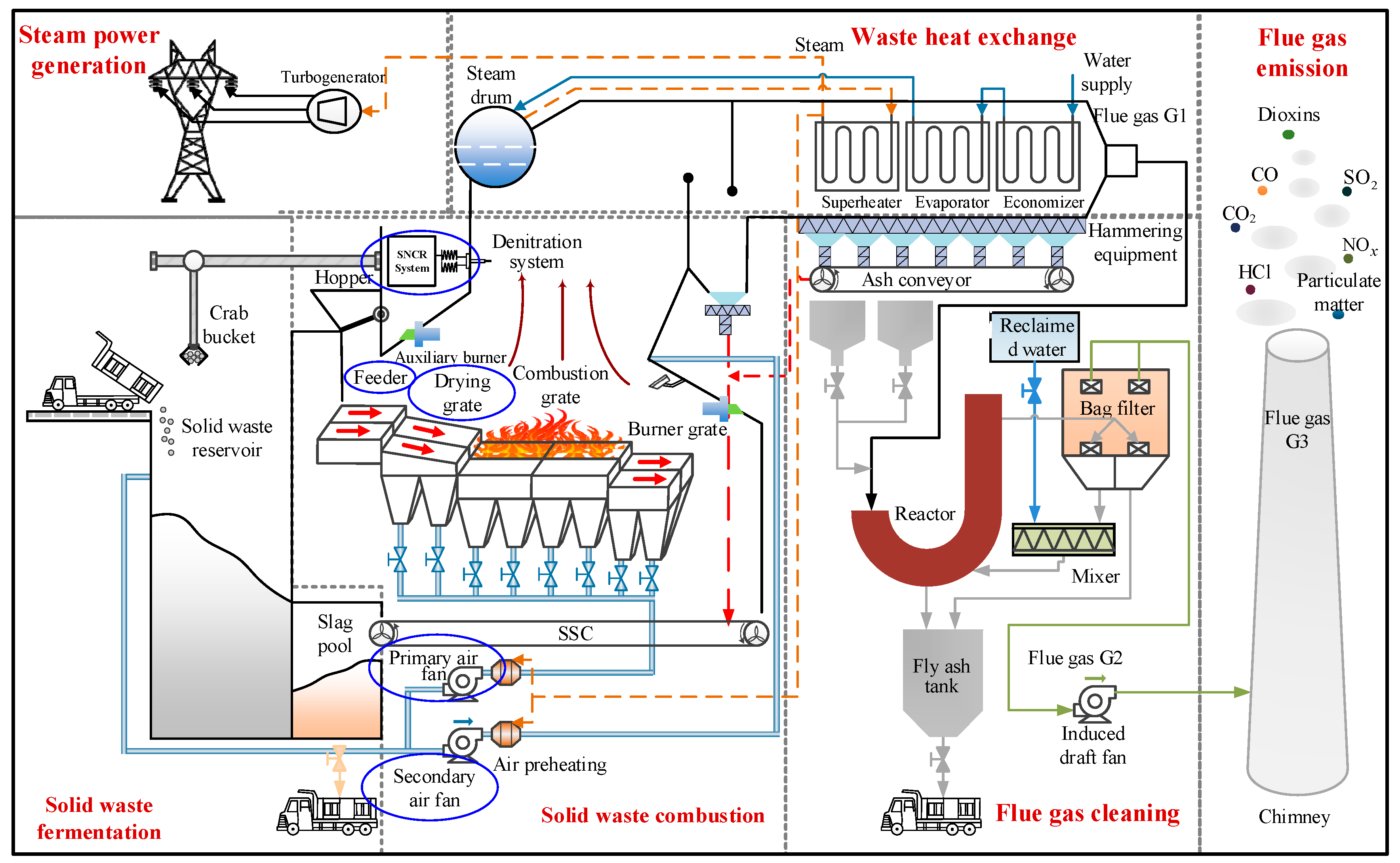
Figure 1. Process flow of the MSWI plant.
Sustainability 17 10577 g001
Figure 2. Dual-layer optimization control framework structure.
Sustainability 17 10577 g002
Figure 3. Schematic diagram of upper-level population initialization encoding.
Sustainability 17 10577 g003
Figure 4. Schematic Diagram of Lower Population Initialization Encoding.
Sustainability 17 10577 g004
Figure 5. Upper-level optimization algorithm fitness variation curve.
Sustainability 17 10577 g005
Figure 6. Pollutant concentration variation with the number of iterations.
Sustainability 17 10577 g006
Figure 7. Optimization algorithm fitness variation curve for the lower layer.
Sustainability 17 10577 g007
Figure 8. Variation curves of four controller parameters with iteration number.
Sustainability 17 10577 g008aSustainability 17 10577 g008b
Figure 9. Algebraic variation curve over 30 iterations reaching the optimal solution.
Sustainability 17 10577 g009
Figure 10. PID control curve under manual and dual-layer optimized tuning.
Sustainability 17 10577 g010
Figure 11. Distribution of convergence generations for the GA.
Sustainability 17 10577 g011
Figure 12. Distribution of generations to optimum for the PSO algorithm.
Sustainability 17 10577 g012
Table 1. Genetic Algorithm Parameter Table.
ParametersUpper-LevelLower-Level
Population Size3050
Maximum Number of Iterations5020
Crossover Probability0.80.8
Mutation Probability0.20.1
Table 2. NOx and CO2 maximum and minimum emission values.
Maximum Emission ConcentrationMinimum Emission Concentration
NOx245.3532 mg/m351.0312 mg/m3
CO210.1750%6.4454%
Table 3. FT Setpoint Range.
Maximum Set ValueMinimum Set Value
r FT * 950 °C900 °C
Table 4. Results of 30 independent runs: Average and Variance.
Upper-Level
Runtime (s)1.9051 ± 0.0115
Optimal Fitness0.3869 ± 0.0000
Generations to Optimal Solution50 ± 0
Table 5. Controller PID parameter ranges.
Control Loop K p Scope K i Scope K d Scope
SAVF(0,5)(0,0.2)(0,2)
ASF(0,3)(0,0.3)(0,1)
ASD(0,4)(0,0.4)(0,2)
AWJ(0,2)(0,0.1)(0,1.5)
Table 6. Optimal multi-loop PID controller parameters.
Control Loop K p  Value K i  Value K d  Value
SAVF0.897901.3187
ASF2.4720.27280.863
ASD1.0480.20360.5158
AWJ1.88620.08491.0332
Table 7. Shared memory update threshold settings.
ParametersValues
θ FT 1
θ NOx 2.5
θ CO 2 0.5
Table 8. Average ± variance of 30 algorithm runs.
Average ± Variance
Optimal Fitness0.4622 ± 0.3263
NOx Concentration60.9998 ± 7.6801
CO2 Concentration8.3003 ± 1.6351
Optimal Temperature Setting935.77 ± 1.57 °C
Table 9. Optimal fitness values under different residuals.
Residual ValueOptimal Fitness
−53.523
03.586
53.629
Table 10. Optimal PID parameters obtained with a residual value of −5.
Control Loop K p K i K d
SAVF1.53830.56920.3721
ASF2.19130.42340.4889
ASD0.98160.15120.5805
AWJ0.50180.08060.7386
Table 11. Optimal PID parameters obtained with a residual value of 0.
Control Loop K p K i K d
SAVF2.87280.15040.5397
ASF1.940800.5493
ASD1.17520.04510.1085
AWJ0.60910.07080.6325
Table 12. Optimal PID parameters obtained with a residual value of 5.
Control Loop K p K i K d
SAVF1.56710.15100.0566
ASF2.99070.16030.7423
ASD0.98660.20330.1268
AWJ0.09720.03581.4827
Table 13. ITAE Values of Control Algorithms by Temperature Stage.
ITAE GA_PID ISNA_PID PID
Stage 1(Original–900 °C)14.91502.381606.15
Stage 2(900 °C–925 °C)29.761331.654898.39
Stage 3(925 °C–910 °C)28.98926.972939.92
Stage 4(915 °C–920 °C)14.92564.241959.58
Stage 5(920 °C–940 °C)25.891075.303918.86
Stage 6(940 °C–930 °C)18.50601.551959.87
Stage 7(930 °C–925 °C)8.82295.55979.9
Table 14. Statistical results of controller performance.
AlgorithmISEIAEDEVmax
GA_PID0.15420.011325
ISNA_PID0.42580.061225
PID1.11480.130125
Table 15. Comparison of Convergence Performance between GA and PSO.
GAPSO
Average Computation Time (s)1.90515.0388
Variance of Computation Time (s)0.01150.1209
Average Generations to Find Optimum4.632.33
Variance of Generations to Optimum41.754.82
Minimum Generations to Optimum11
Maximum Generations to Optimum2810
Disclaimer/Publisher’s Note: The statements, opinions and data contained in all publications are solely those of the individual author(s) and contributor(s) and not of MDPI and/or the editor(s). MDPI and/or the editor(s) disclaim responsibility for any injury to people or property resulting from any ideas, methods, instructions or products referred to in the content.