Article

Effects of Land Use Change on Ecosystem Service Dynamics in the Guangxi Xijiang River Basin

1
Key Laboratory of Environmental Change and Resources Use in Beibu Gulf, Ministry of Education, Nanning Normal University, Nanning 530001, China
2
Guangxi Key Laboratory of Earth Surface Processes and Intelligent Simulation, Nanning Normal University, Nanning 530001, China
3
School of Management Science and Engineering, Guangxi University of Finance and Economics, Nanning 530003, China
*
Author to whom correspondence should be addressed.
Sustainability 2025, 17(23), 10558; https://doi.org/10.3390/su172310558
Submission received: 15 September 2025 / Revised: 10 November 2025 / Accepted: 21 November 2025 / Published: 25 November 2025

Abstract

This study assessed how spatiotemporal changes in land use dynamics affect ecosystem services responses using land use data (1990–2020) from the Guangxi Xijiang River Basin. The results indicate that cropland, forest, water, barren, and impervious areas increased 0.18%, 1.28%, 14.9%, 636.54%, and 208.03%, respectively, while shrubland and grassland decreased by 43.02% and 80.61%. Spatially, vegetation cover was higher in the eastern, northern, and western sections, whereas the central and southern regions were dominated by cropland and impervious surfaces. Water yield, habitat quality, carbon storage and soil conservation decreased by 13.38%, 9.75%, 7.43% and 10.77%, respectively, with notable decreases in the northeastern, eastern, and northwestern areas. The total amounts of these services were 15.06 × 10¹⁰ m3, 0.45, 17335TgC and 9.42 × 10¹⁰ t, respectively. Land use changes affected ecosystem services as follows: cropland and impervious areas enhanced water yield but reduced habitat quality, carbon storage and soil conservation; forests, shrublands, and grasslands promoted the regulation and support services related to carbon storage, habitat quality and soil conservation; wetlands improved habitat quality and soil conservation; and water and barren land had limited impacts relative to other land types. This study addresses a methodological gap in dynamic ecosystem service assessment in the Guangxi Xijiang River Basin and offers insights into integrated land and ecosystem management.

1. Introduction

Ecosystem services are defined as the direct and indirect products and provisions from the structure and workings of ecosystems [1,2,3]. These services are formed by the supporting, provisioning, regulating, and cultural functions of ecosystems and their interactions [1]. Accelerated socioeconomic development has driven transformations in land use configurations, leading modifications in ecosystem composition and operational dynamics, thereby affecting the capacity of ecosystems to deliver services [4,5]. Therefore, a systematic analysis of land use, ecosystem services, and their interrelationships provides valuable insights for rationally planning land use, optimizing national territorial spatial patterns, guiding ecological policy formulation and implementation, and promoting sustainable ecosystem development.
In recent years, the evaluation of ecosystem services mainly focuses on the evaluation of individual ecosystem services [6], the comprehensive analyses using coupled models [7], the coordination and trade-offs, and connections to human well-being [8]. Among various ecosystem assessment frameworks, the Integrated Valuation of Ecosystem Services and Tradeoffs (InVEST) model [9] stands out as the most comprehensive and well-developed, offering the most extensive suite of assessment modules [7]. Most studies have focused on land use changes or ecosystem services at the regional scale or for specific land use types [10,11], often overlooking whether land use changes driven by economic policies within river basins could induce variations in the spatial heterogeneity of ecosystem services. Furthermore, the interrelation of land use patterns with ecosystem service capacities was shaped by spatiotemporal variations. Studies by Xun Rui and other scholars have shown that intensified land use development significantly contributes to the degradation of regional ecosystem services [12,13,14,15]. Current research in the Guangxi Xijiang River Basin has predominantly emphasized ecosystem service valuation [16,17], whereas there has been a lack of sufficient focus on how land use transformations impact such services across the basin [18]. Therefore, long-term studies are necessary for assessing the spatiotemporal dynamics of land use alterations’ effects on ecosystem services in the Xijiang River Basin, clarifying their relationships, and enhance ecosystem service benefits.
The Guangxi Xijiang River Basin serves as a vital transportation hub situated within a critical zone of China’s southern ecological barrier. It is rich in natural resources and provides essential services comprising water and soil conservation, biological diversity support, and climate adjustment [19]. This study sets three primary purposes: (1) to explore how land use transitions evolve in spatiotemporal patterns and how ecosystem services changes across the basin; (2) to reflect the multi-year average level of ecosystem service supply capacity using Getis-Ord Gi* hot spot analysis; and (3) to delineate how ecosystem service functions are spatially linked to land use change dynamics through bivariate spatial autocorrelation analysis. The results of this research are conducive to watershed sustainability studies and offer a scientific basis for the optimization of regional land use patterns, rational water resource utilization, and ecosystem management.

2. Materials and Methods

2.1. Research Framework

This research builds a framework analyzing land use change and ecosystem services (Figure 1). With land use functioning as a vital bridge connecting natural and human systems, its long-term shifts bring about alterations to ecosystem services. Through spatiotemporal analysis, we identified the interconnections between ecosystem services and land use. Drawing on these research findings, we put forward targeted suggestions and countermeasures to regulate human activities and promote ecological conservation in the Guangxi Xijiang River Basin.

2.2. Study Area

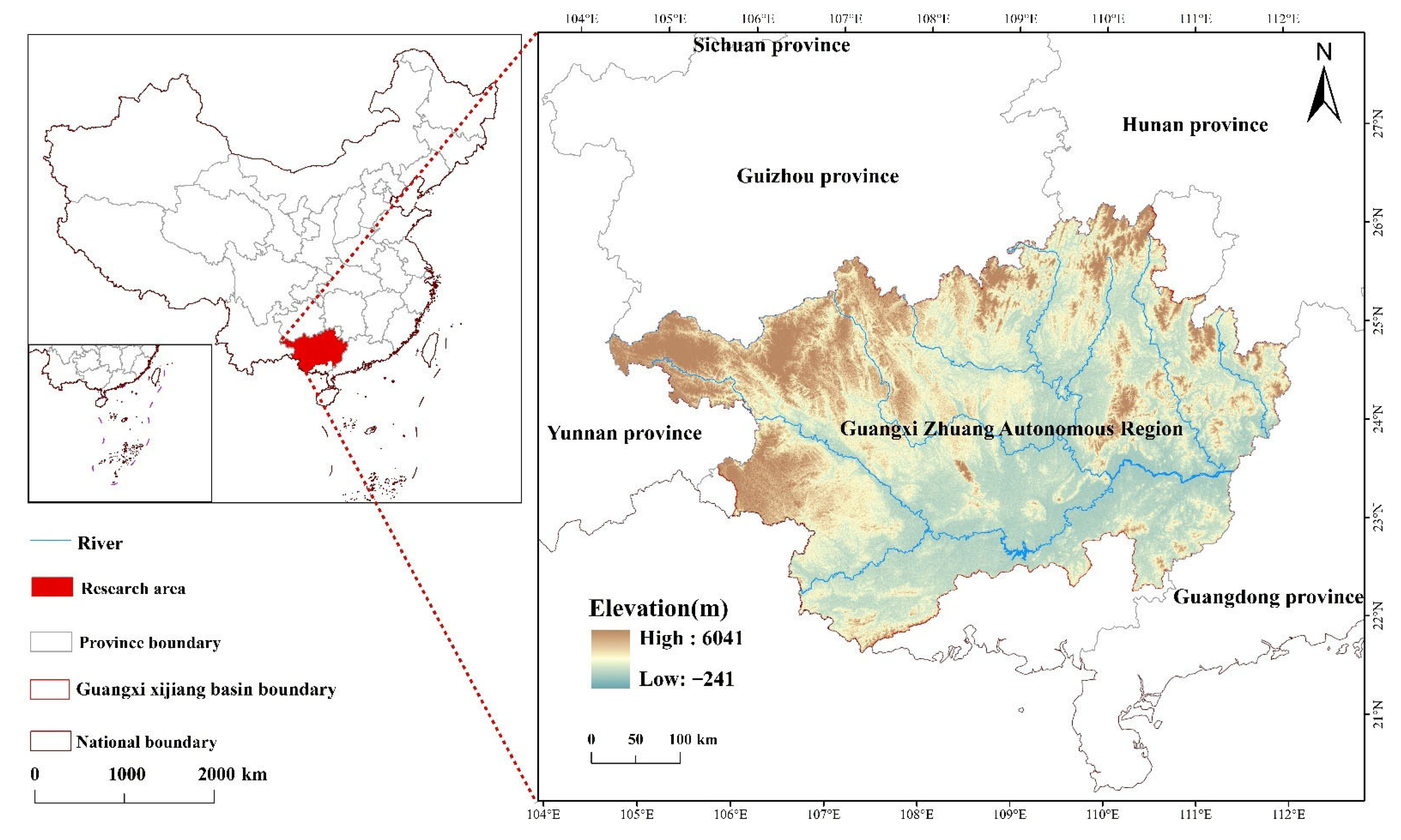
The Guangxi Xijiang River Basin (104°28′ E–112°04′ E, 21°35′ N–26°20′ N) is in southwest China, covering an area of 20.31 × 10⁴ km2. The basin features a characteristic basin-and-valley topography, with mountainous peripheries enclosing narrow alluvial plains along river valleys. This fragmented basin landscape is predominantly composed of mountainous hills, with limited plain areas and well-defined basin morphology (Figure 2). It exhibits favorable thermal conditions with synchronous peaks in temperature and precipitation, with a mean annual temperature of 16.5–23 °C and mean precipitation of 1080–2760 mm [20].

2.3. Acquisition of Data and Preprocessing Procedures

2.3.1. Land Use and Cover Dataset

The land use and cover data were obtained from the Annual China Land Cover Dataset (CLCD) [21] (https://zenodo.org/record/4417801#.YSpGFI4zaUn; accessed on 22 January 2024) with a spatial resolution of 30 m. The dataset’s land use classification comprises nine types: cropland, forest, shrub, grassland, water, snow/ice, barren, impervious, and wetland. In line with this study’s needs, we focused on eight relevant categories, excluding snow/ice due to its absence within the research zone.

2.3.2. Meteorological Data

From the National Earth System Science Data Center (https://www.geodata.cn; Accessed on 10 May 2024), we retrieved the meteorological datasets employed for this study, including three types of datasets with a 1 km resolution: annual average temperature data (1982–2022), annual precipitation data (1982–2022), and monthly potential evapotranspiration data (1901–2022).

2.3.3. Relevant Supplementary Data

30 m spatial resolution DEM datasets were acquired from the Geospatial Data Cloud (https://www.gscloud.cn/; accessed on 28 May 2024). We retrieved HWSD from the National Tibetan Plateau Data Center, which has a spatial resolution of 1 km (http://data.tpdc.ac.cn; accessed on 29 May 2024). From China’s 100 m Depth-To-Bedrock map (DTB), we retrieved the root restriction layer depth (http://globalchange.bnu.edu.cn/research/cdtb.jsp; accessed on 11 July 2024).

2.3.4. Data Preprocessing

All data underwent unification to a spatial resolution of 30 m × 30 m, with WGS1984 UTM Zone 49N adopted as the projection coordinate system. Processing began with importing the raw data into ArcGIS 10.8 and defining its coordinate system through projection to WGS1984. Subsequently, all datasets were uniformly projected to the WGS1984 UTM Zone 49N. Resampling was performed on the raster datasets to attain a uniform 30 m spatial resolution, thus laying the groundwork for a basic map of the research region in subsequent analyses.

2.4. Research Methodology

2.4.1. Investigation into the Dynamics of Land Use

Transfer Matrix
We employed the transfer matrix to capture the spatial–temporal transitions between different land cover categories within the Guangxi Xijiang River Basin during 1990–2020. Specifically, it was derived using the ArcGIS 10.8 Raster Calculator and the Excel 2013 Pivot Table tools [22]. Below is the corresponding Formula (1):
S l ˙ j = S 11 S 12 S 1 n S 21 S 21      S 2 n         S n 1   S n 2    S n n
In this formula, Sij refers to the overall area of national land space shifted from type i to type j at the start of the study, and n represents the count of land use categories.
Land Use Intensity
Human utilization and modification of land define land use intensity as the corresponding degree. The comprehensive index of land use intensity quantifies human disturbance by assigning weighted values to different land cover categories based on their ecological transformation levels. This index effectively integrates the natural carrying capacity of land together with the cumulative impacts resulting from human use patterns [23]. Below is the specific Formula (2):
L = 100 × i = 1 n A i × C i
where L represents the comprehensive index of land use intensity; Ai, the classification index of land use types (refer to Supplementary Material S1); Ci, the proportion of class i area; n, the count of classification levels. The land use intensity index exhibits a positive correlation with anthropogenic disturbance levels, where lower index values signify minimal human modification of natural landscapes, while higher values indicate substantial anthropogenic transformation of terrestrial ecosystems.

2.4.2. Quantitative Assessment of Ecosystem Services

The InVEST model was utilized to assess four ecosystem services, including water yield, soil conservation, carbon storage, and habitat quality. The InVEST facilitates comprehensive spatial quantification of ecosystem services through its modular assessment framework [24]. The expressions are shown in Equations (3)–(6) (Figure 2). Further, the specific operational methods can be referenced in the user guide for InVEST (https://naturalcapitalproject.stanford.edu/software/invest, accessed on 28 May 2024).
This study employed the InVEST model (version3.14.1), elaborates on the model’s parameter selection process, and determined the parameter values based on relevant studies conducted in the adjacent regions of the Xijiang River Basin in Guangxi (refer to Supplementary Material S2). With respect to the relevant parameter values of the Soil Conservation module, it is hereby clarified: we selected the Seasonal Delivery Ratio module in the InVEST model as the data processing component for soil conservation analyses. When utilizing this module, the values of Threshold Flow Accumulation (number of pixels), Borselli K Parameter, Maximum SDR Value, Borselli IC0 Parameter, and Maximum L Value were sequentially set to 1000, 2, 0.8, 0.5, and 122. Detailed information on all input parameters is provided in Material S3. We have conducted statistical tests to verify the significance of changes in ecosystem services over time, as detailed in Supplementary Material S4.
Water yield (WY). The formula is as follow:
W Y ( x ) = 1 A E T ( x ) P x     P x
In the formula: WY(x) is the annual water yield (mm); AET(x) refers to the annual actual evapotranspiration (mm) at grid cell x; and P(x) corresponds to the annual precipitation (mm) at grid cell x [25].
Soil conservation (SC). The formula is as follow:
Q S r = Q s e p Q s e a
Q s e p = R     K     L S
Q s e a = R     K     L S     C     P
where Qse−p represents potential soil erosion quantity; Qse−a, the actual soil erosion quantity; R, the rainfall erosivity factor; K, the soil erodibility factor; LS, the slope length factor; P, the soil and water conservation measure factor; and C, the vegetation coverage and management factor [26].
Carbon storage (CS). The formula is as follow:
C t o t = C a b o v e + C b e l o w + C S o i l + C d e a d
where Ctot is the total carbon storage; Cabove demotes the aboveground biomass carbon; Cbelow signifies the belowground biomass carbon density; Csoil represents the soil carbon density; and Cdead indicates the litter organic matter carbon density [27].
Habitat quality (HQ). The formula is as follow:
H Q x j = H j × 1 D x j z D x j z + k z
where HQxj stands for the habitat quality of pixel x with land use type j; Hj, the habitat suitability corresponding to land use type j; Dxj, the habitat degradation level of pixel x under land use type j; k, a half-saturation constant (k = 0.5); and Z is defined as 2.5 in the model [28].

2.4.3. Cold and Hot Spot Analysis

Within the ArcGIS 10.8 platform, cold-hot spot analysis was implemented utilizing the local Getis–Ord Gi index technique. This approach statistically evaluates whether high- or low-value clusters exhibit significant spatial aggregation. Results visualization helps identify clustered high- and low-value zones [29].
The values of each ecosystem service were assigned to a 5 km fishnet to create mean value layers representing the 30-year period from 1990 to 2020. These layers were then analyzed via the Getis–Ord Gi* analytical tool within the ArcGIS 10.8 platform to identify spatial patterns. Our results explicitly reveal how ecosystem service supply capacity is spatially distributed in the study area, emphasizing the clustering of high-and low-value regions [30]. Provided below is the Formula (7):
  G * = i = 1 n Q i j a ¯ i = 1 n Q i j i = 1 n a i 2 n a 2 i = 1 n Q i j 2 i = 1 n Q i j 2 n 1
where G* is the aggregation index of raster i; ai refers to the attribute value of a given raster i; n signifies the total unit count; a ¯ corresponds to the mean value of the total ecosystem service functions of all pixels; and Qij is the weight matrix. A high positive G* points to a hot spot, in contrast to a negative G* that corresponds to a cold spot. The magnitude of the G* statistic reflects the intensity of clustering, with higher values indicating tighter and more statistically significant agglomerations.

2.4.4. Bivariate Spatial Autocorrelation Analysis Method

Spatial autocorrelation analysis evaluates the dependency between variable distributions in geographic units and their neighbors. It includes global spatial autocorrelation, which assesses overall spatial patterns across the study area, and local spatial autocorrelation, which identifies localized clusters or outliers. For multi-variable relationships, bivariate spatial autocorrelation examines spatial associations between paired variables [31].
I k l = n σ = 1 n σ j 1 n W i j Z K i Z I j n 1 σ = 1 n σ j 1 n W i j
I K I l ˙ = Z K i σ j = 1 n W i j Z I j
where Ikl and I k l i is the bivariate global Moran’s I index and local Moran’s I index, respectively; n denotes the total count of spatial units within the study area; Wij stands for the corresponding spatial weight matrix; and Z K i and Z I j are the standardized values of attributes K and L for units i and j, respectively.

3. Results

3.1. Spatiotemporal Patterns and Variation in Land Use in Guangxi Xijiang River Basin

The primary categories of land use within the Guangxi Xijiang River Basin are cropland, forest, and shrub, which cover 98% of the basin (Figure 3). Forests represent the dominant land cover type within the research area, comprising 71.77% of the area’s total surface. Shrublands and grasslands display an intermixed distribution pattern, primarily distributed across mid–low elevation mountainous regions and the western basin plains. Concentrated in the flat plains and basins across the central and southern regions are croplands, with smaller scattered patches distributed along the upper reaches of the eastern Luoqing River as well as the river networks of the Lijiang and Hejiang. Impervious surfaces are largely confined to urban and peri-urban areas, particularly around administrative centers such as Nanning, Liuzhou, and Guilin. Wetlands and water bodies, covering a limited area, and are scattered throughout.
The study period (1990–2020) was marked by a general stability in the spatial arrangement of land use types, with only minor fluctuations in their respective areas. However, notable conversions occurred between cropland and forest, cropland and shrubland, and cropland and impervious surfaces. These changes suggest a land use pattern characterized by broad stability at the regional scale, alongside localized areas of significant transformation.
The transfer matrix analysis demonstrated notable bidirectional conversions between cropland and forest, as well as between shrubland and forest, representing the most prominent land use change patterns in the basin (Figure 4). Quantitatively, forest-to-cropland and forest-to-shrub conversions accounted for 10,153.9 km2 and 1451.19 km2, respectively, while reverse conversions (cropland-to-forest and shrub-to-forest) covered 8962.63 km2 and 4407.65 km2.
Impervious surfaces showed a steady spread, mainly within urban areas (e.g., Nanning, Liuzhou, Guilin), characterized by flat terrain and high population density, as well as along the riparian zones of major river networks (Yujiang River, Hongshui River, middle–lower Liujiang River, Qianjiang River, and Xunjiang River). From 2010 to 2020, rapid expansion was observed in impervious surfaces, with a total growth of 1648.946 km2 (a 208.03% increase), predominantly through the conversion of cropland (1511.14 km2) and forest (174.93 km2). Impervious surfaces showed limited conversion to other land types, transitioning primarily to cropland (1.68%) and water bodies (8.46%).
From 1990 to 2020, the Guangxi Xijiang River Basin experienced notable land use changes: cropland, forest, water bodies, barren land, and impervious surfaces exhibited net increases, whereas shrubland and grassland areas declined.

3.2. Spatiotemporal Variations in Ecosystem Service Functions

Over the 1990–2020 period, the Guangxi Xijiang River Basin exhibited distinct temporal patterns in ecosystem services. Exhibiting a comparable nonlinear tendency were both water yield service and soil conservation service: a decline in the initial phase, with a subsequent period of improvement, and a later reduction. By the end of the period, the two services had experienced net reductions of 13.38% and 10.77%, respectively (Figure 5a,b). In contrast, carbon storage and habitat quality demonstrated a consistent downward trend, declining by 7.43% and 9.76% from 1990 to 2020 (Figure 5c,d).
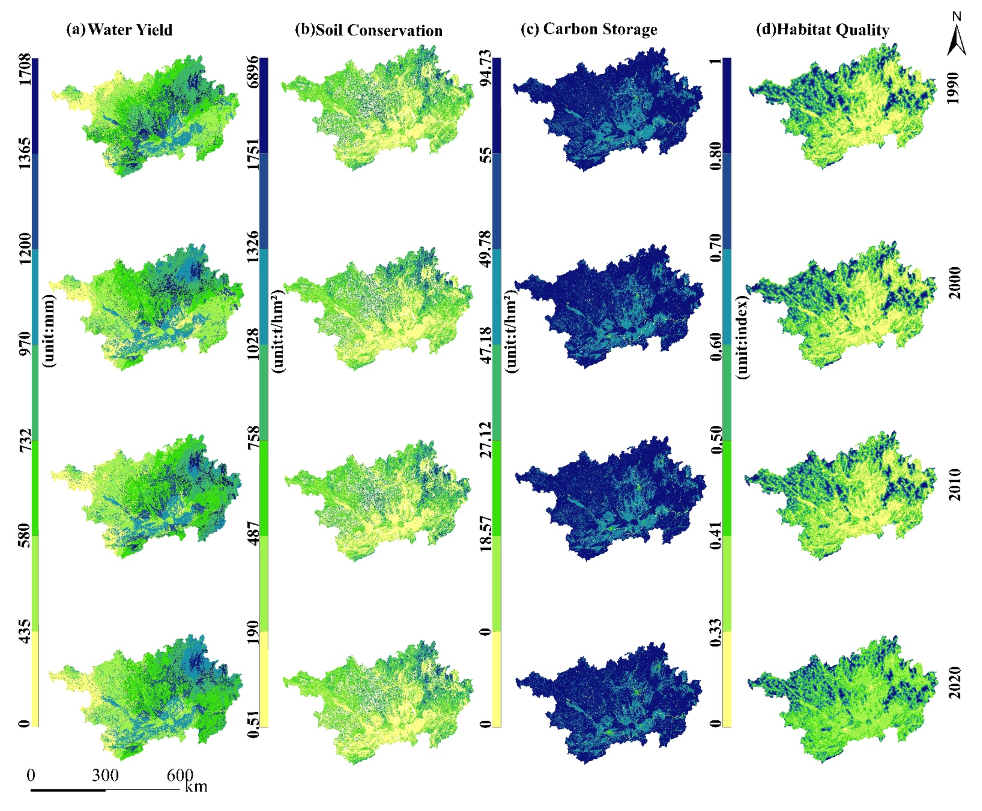
From 1990 to 2020, water yield capacity exhibited a notable spatial distribution, with relatively low levels in the northwest and southeast regions, comparatively high levels along the southwest-to-northeast diagonal, and a gradual decrease from west to east (Figure 6a). High water yield areas extended from the southwest to the northeast, covering Chongzuo, Nanning, Laibin, Liuzhou, and Guilin City. Over the 30-year period, these areas were consistently concentrated in a zone stretching from Rong’an County (Liuzhou) to central Guilin, with values around 1365 mm or higher. Low-water-yield areas were mainly distributed along the northwestern edge of the basin, particularly in the Napo–Xilin–Tian’e County as well as in the southwestern sector, spanning the Daxin County–Pingxiang County corridor, where water yield was approximately 435 mm or lower.
Distinct spatial heterogeneity was observed in soil conservation, characterized by enhanced capacities in the northeast and reduced capacities in the central-south (Figure 6b). High-value soil conservation areas were primarily distributed in ethnic autonomous counties north of Liuzhou (northeastern of the Basin) and mid–low mountains in Guilin (excluding Guilin’s urban area and Lingui District surroundings). Smaller patches also scattered in Jinxiu Yao Autonomous County (eastern Laibin) and Hezhou. The soil conservation quantity in these high-value areas was approximately 1751 t/hm2 or higher. In contrast, low-value areas (approx. 190 t/hm2 or less) were mainly distributed across the central plain regions south of Liuzhou City, including parts of Laibin, as well as areas around Nanning and Guigang cities.
An evident spatial pattern was presented by the carbon storage capacity, with higher levels in outer zones and lower levels in the central region (Figure 6c). High-value carbon storage areas (exceeding 55 t/hm2) exhibited a scattered distribution pattern, with the majority concentrated in the basin’s northeastern and eastern regions. In contrast, low-value areas—with carbon storage levels below 18.5 t/hm2—were distributed in an inverted “T” shape, concentrated in and around central and southern basin cities, including Chongzuo, Nanning, Laibin, Guigang, Liuzhou, and Guilin.
Habitat quality exhibits a spatial distribution pattern highly consistent carbon storage (Figure 6d). High-habitat-quality zones (index > 0.80) were predominantly distributed in the northwest basin, extending eastward to Jinxiu Yao Autonomous County, Zhaoping, Cangwu, Pinggui, and Babu Districts. Additionally, scattered patches were observed in the northeast, including Rongshui, Sanjiang, and Longsheng. In contrast, low-value areas (index < 0.33) were concentrated in urban centers and surrounding areas of Liuzhou, Guilin, Chongzuo, Nanning, Laibin, Guigang, and Wuzhou, situated in the central, northeastern, and southern parts of the basin.

3.3. The Interrelationship Between Land Use Patterns and Ecosystem Services

3.3.1. Effects of Different Land Use Types on Ecosystem Service Supply

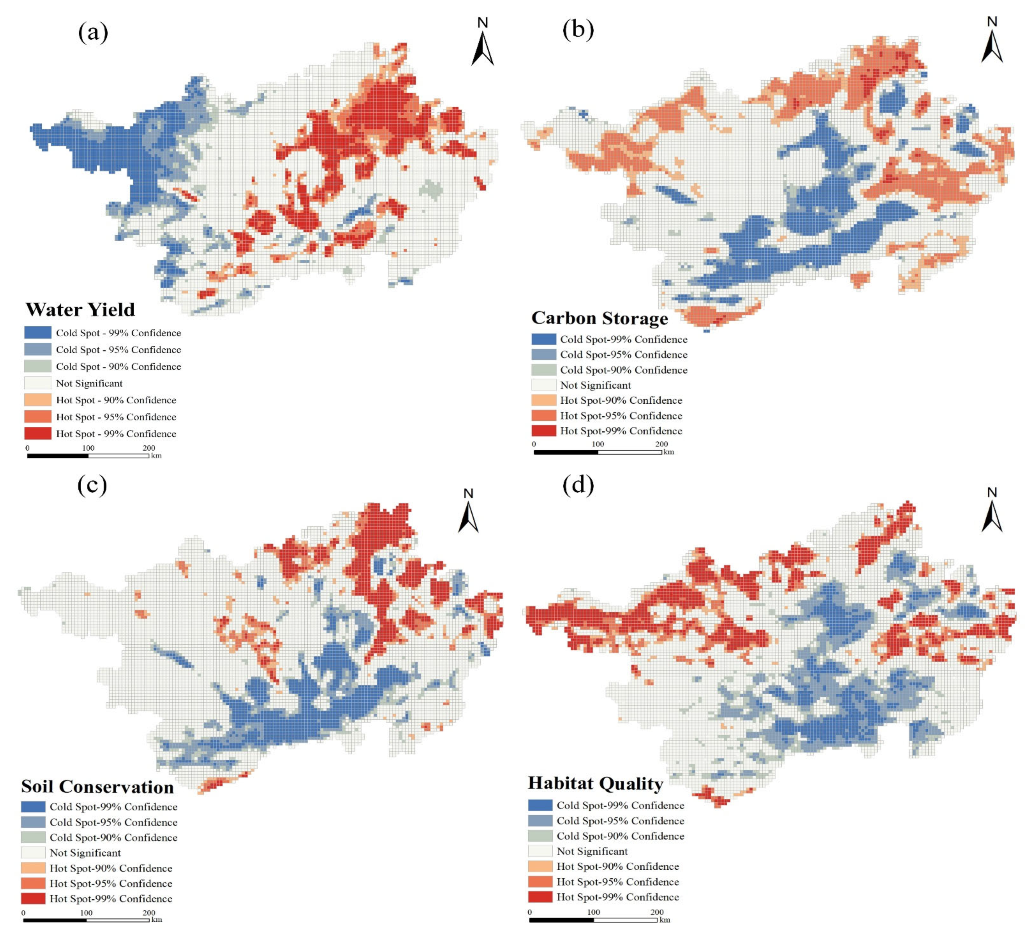
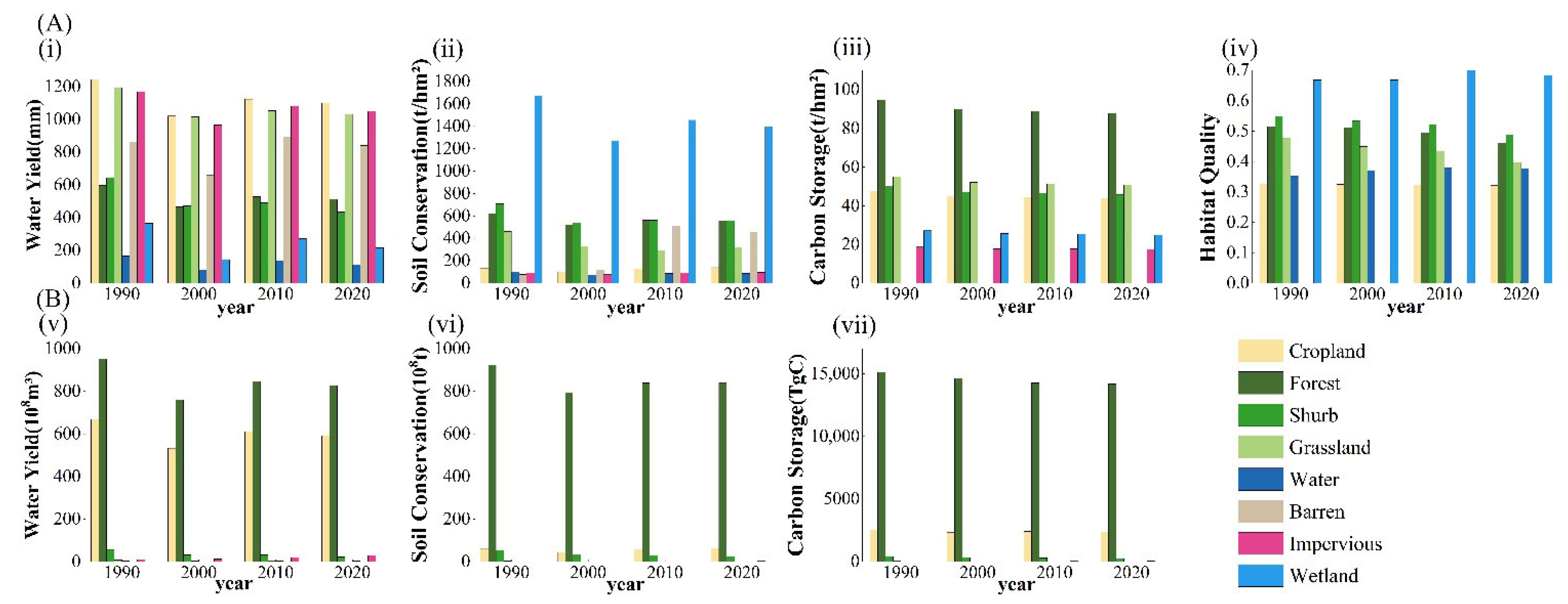
In terms of water yield services, distinct spatial heterogeneity existed, where values in the eastern regions were considerably higher than those in the western areas (Figure 7a). High water yield value was predominantly associated with cropland, grassland, and impervious surfaces, with average values of 1122.64 mm, 1074 mm, and 1067.31 mm, respectively (Figure 3 and Figure 8A(i)). In contrast, the low water yield occurred in the west and central–southern, particularly within the Yujiang River, Zuojiang River, and Qianjiang River watersheds, where the average water yield was 123.91 mm.
Higher soil conservation capacity is found in the northeast and lower capacity in the south. A small fraction is distributed in the central, where land cover is dominated wetlands (Figure 7b). Forestland is the predominant type of land use in the northeast (Figure 3). Forest vegetation, through its extensive root systems, contributes to soil stabilization and thereby promotes sediment retention [32]. Wetlands in the central basin also played a critical role in soil conservation. Slow water flow facilitated sediment deposition, while diverse wetland vegetation stabilized the accumulated sediments. The average soil conservation amounts of wetlands, shrublands, and forestlands were 1499.93 t/hm2, 591.935 t/hm2, and 565.44 t/hm2, respectively (Figure 8A(ii)). The southern area is mainly composed of cropland and built-up areas, where green infrastructure is limited. These land use types reduced the capacity for soil conservation [33].
Spatial analysis revealed a clear periphery-core gradient in both carbon storage and habitat quality, with elevated measurements in outer zones and diminished quantities toward the center (Figure 7c). High-value areas for carbon storage were primarily covered by forestland, grassland, and shrubland, with average values of 90.27 t/hm2, 52.33 t/hm2, and 47.40 t/hm2, respectively (Figure 3 and Figure 8A(iii)). Similarly, high-value areas for habitat quality were mainly associated with wetlands, shrubland, and forestland, averaging 0.68, 0.52, and 0.50, respectively (Figure 3, Figure 6d and Figure 8A(iv)). Notably, forestland, cropland, and shrubland serve as the primary stable sources of ecosystem services of the basin, accounting for 98.41%, 99.67%, and 99.73% of the total service supply in water yield, soil conservation, and carbon storage, respectively (Figure 8B).

3.3.2. The Influence of the Composite Index for Land Use Degree on Ecosystem Services

The bivariate spatial autocorrelation results (Table 1) revealed statistically significant clustering patterns (all p = 0.001), rejecting the null hypothesis of random spatial distribution. The average Moran’s I value for the integrated land use intensity index and the water yield ecosystem service was 0.44, indicating positive spatial autocorrelation between these two variables. Moreover, the average Moran’s I values between land use intensity and soil conservation, carbon storage, and habitat quality were −0.36, −0.62, and −0.45, respectively, indicating negative spatial correlations. The spatial correlations were grouped into four clustering categories, specifically High–Low(H–L), High–High(H–H), Low–Low(L–L), and Low–High(L–H).
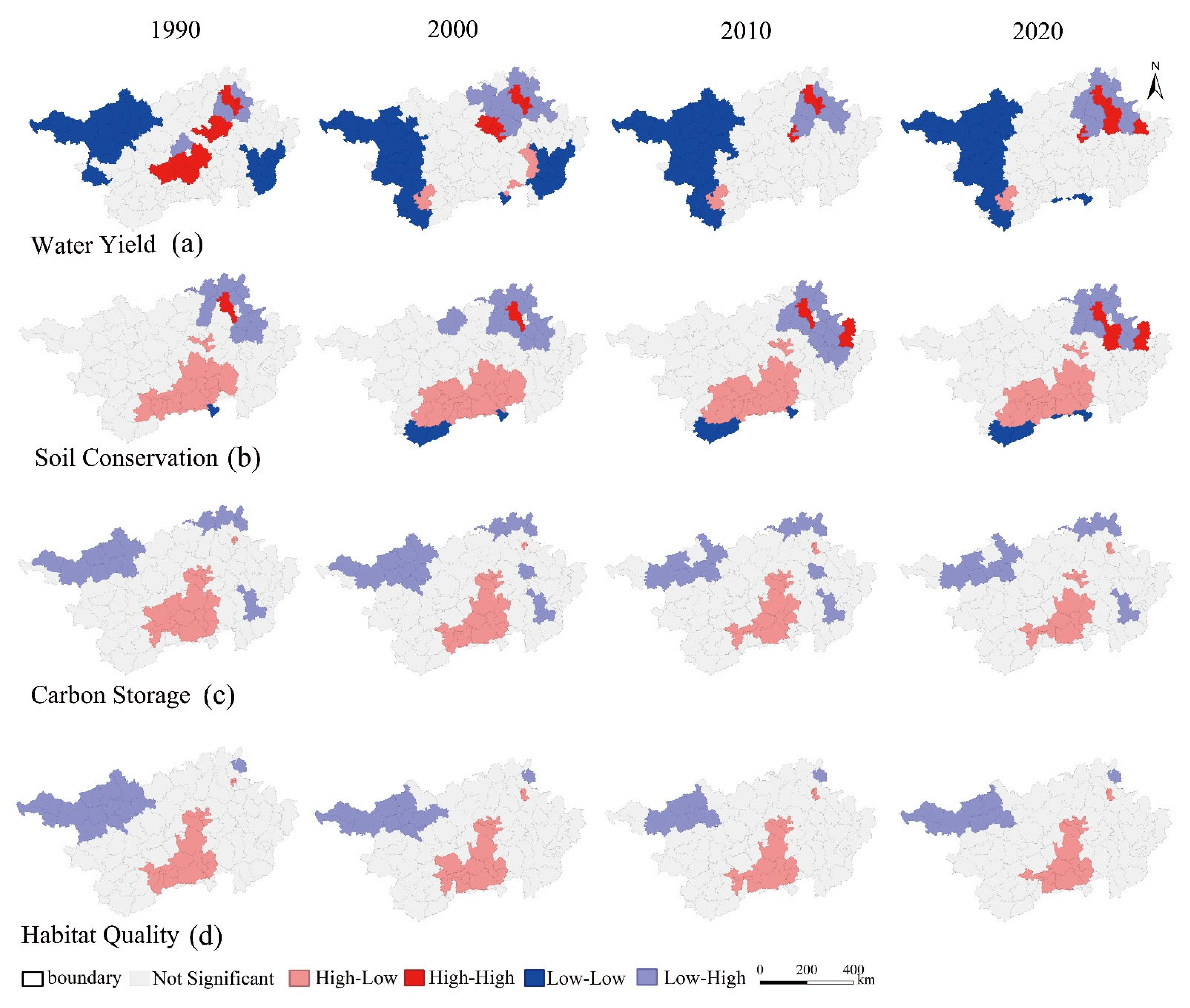
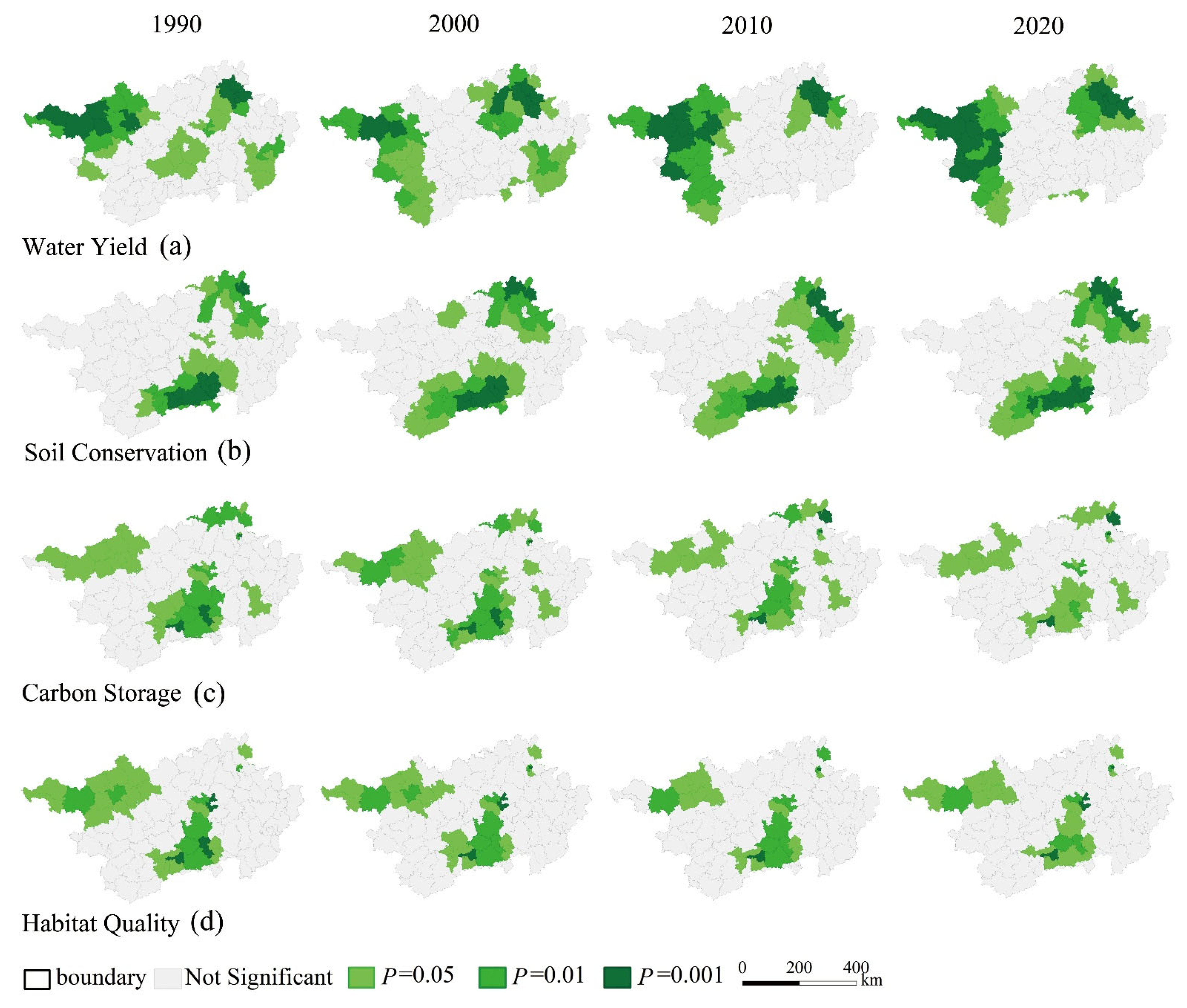
Utilizing results of spatial bivariate autocorrelation (Figure 9 and Figure 10), we generated LISA cluster and significance diagrams to illustrate the interrelationship of land use intensity with ecosystem services.
Throughout the 1990–2020 period, the bivariate spatial correlation between land use intensity and water yield was primarily observed in the eastern and western parts of the basin, with limited presence in the central region. The local spatial autocorrelation pattern exhibited high east and low west clustering, while the global significance pattern showed high north and low south differentiation (Figure 9a and Figure 10a).
H-H clustering was observed in 19 districts and counties—such as Lingui, Yanshan, and Yangshuo—accounting for 18.45% of the region. Among them, seven areas, including Lingui and Xiangshan, showed particularly strong significance (Figure 10a, p = 0.001). The integrated index for land use intensity and the water yield ecosystem service in this region both exhibited relatively high values, indicating a synergistic relationship between the two. High-level areas were clustered in southwestern Liuzhou City and the central–western part of the Lijiang River Basin. However, the extent of these synergistic regions has reduced over the course of the research. Expansion of urban areas and tourism development in Liuzhou and Guilin have intensified land use changes, resulting in a pronounced trade-off trend [34,35,36]. Conversely, L-L clustering occurred in 30 counties—such as Xilin, Longlin, and Tianlin—making up 30.10% of the study area (Figure 9a). These regions were marked by comparatively low water yield capacity and land use intensity levels.
Throughout the research period, the clustering pattern between land use intensity and soil conservation was primarily observed in the northeastern part of the basin (Figure 9b). H-H clustering occurred in Lingui, Fuchuan, Zhongshan, Yangshuo, and Lipu, these areas constituted 4.85% of the total study area. A growing trend of this pattern was observed over the 1990–2020 timeframe. Specifically, soil conservation functions and land use intensity featured a coordinated development pattern within the Guilin-Hezhou area. The implementation of farmland-to-forest conversion policies contributed substantially to the enhancement of synergy within the system [37]. H-L clustering patterns prominently reflected soil conservation and the land use intensity index (Figure 9b and Figure 10b). These clusters were predominantly situated in the southern area of the basin, representing 24.27% of the basin’s total area. Notable regions within this distribution include Gangbei, Qintang, Qingxiu, Yongning, Jiangnan, and Hengzhou City, with statistically significant results (p = 0.001; Figure 10b). These areas exhibited a clear trade-off relationship, with relatively high land use intensity coupled with low soil conservation capacity.
The comprehensive index of land use intensity consistently demonstrates trade-off relationships with both habitat quality and carbon storage, rather than synergistic effects (Figure 9c,d). Primarily situated in the study basin’s south-central region and central Guilin were H-L clusters for these ecosystem functions, while L-H clusters gathered in the basin’s northern area. A modest quantity of L-H clusters related to carbon storage were sporadically distributed within Wuzhou.
The south-central basin and central Guilin were dominated by farmland and built-up areas (Figure 3), leading to ecological trade-offs, where high-intensity land use was associated with compromised carbon sequestration and biodiversity support. The northern clustering zones were dominated by forest and shrubland (Figure 3), which were associated with higher forest coverage [38]. In Wuzhou, local preferences for water quality and forest conservation helped maintain lower land use intensity and higher levels of both carbon storage and habitat quality [39]. The H–L patterns, together with the L–H ones, demonstrate a downward trend, suggesting a gradual weakening of the trade-off relationship.
Regions exhibiting heightened significance (p = 0.01) and statistically significant (p = 0.05) were predominantly distributed near H–H or L–L clusters, indicating indirect geospatial effects (Figure 10). This pattern suggests that ecological services were influenced by adjacent regions. Given the spatial dependence among neighboring areas, attributes of nearby patches have stronger impacts than those farther away. As a result, in counties with either high or low synergy levels, these conditions tend to spread to surrounding areas through spatial spillover effects, eventually forming feedback mechanisms through regional interaction. To address this, land use and ecosystem protection policies should incorporate interregional spillover effects. Regional integration and coordinated resource management should be employed to mitigate imbalances in ecosystem services [40,41].

4. Discussion

4.1. The Integration of Land Use and Ecosystem Services Has Important Implications for Further Research

The framework proposed in this study enables the enhancement of ecosystem services from a land use perspective. Constituents of natural and human-related systems (climatic regimes, terrain characteristics, socioeconomic factors, among others) are extensively interconnected through land use and its shifts [42]. A core objective of SDGs [43] is to conserve ecosystem services, regulate their utilization by human societies, and thereby improve overall well-being [44]. The realization of this goal requires more systematic conservation strategies and action plans. By clarifying the relationship between ecosystem services and land use, tailored governance measures may be formulated to guide land use transition, especially through the modulation of land use modalities, thereby boosting future ecosystem services. In this context, a research framework grounded in evaluating how land use influences ecosystem services delivers an all-round analytical method for successfully tackling eco-environmental predicaments, and simultaneously provides useful implications for regions under comparable conditions.

4.2. The Influence Exerted by Land Use Transition on Ecosystem Services

Between 1990 and 2020, the study underwent significant land use transformations with 28,708 km2 of land converted among different cover type (Figure 4), between. Notable shifts were observed among cropland, forest, and shrubland. Additionally, there was a growing trend of cropland and forest being converted into impervious surfaces, a finding consistent with previous studies in the study area [45]. Such local-scale transformation was mainly driven by urban expansion, the execution of ecological restoration initiatives, and agricultural activities [46]. Within the mid-reaches of the study area, cropland and forest exhibited an interlaced distribution, primarily concentrated in Liuzhou and Laibin Cities (Figure 3). The region is characterized by karst basins and karst peak-cluster depressions, with agriculture serving as the dominant economic sector [47]. Historically, extensive forestlands were converted to cropland. However, the launch of ecological restoration projects—which includes the “Grain for Green” Program and another key initiative, the “Natural Forest Protection Program”—has led to extensive cropland and shrubland being restored to forestland, substantially improving forest resource conservation [40]. Meanwhile, the growing demand for land use associated with human activities has adjusted the structural composition of land use. Impervious surfaces have continued to expand, encroaching upon large tracts of agricultural land and intensifying land development. This process has, to a certain extent, offset the positive feedback of afforestation projects [48] and indirectly contributed to changes in ecosystem services.
The degradation or restoration of ecosystem services is closely linked to land use types [30]. Ecosystem services demonstrated distinct variations across land use types (Figure 7 and Figure 8). High water yield was clustered in cropland, grassland, and construction land. In contrast, habitat quality, carbon storage and soil conservation were highest in forestland, wetlands, and shrubland—ecosystems characterized by minimal human disturbance. This spatial pattern matches findings of studies conducted in comparable watersheds [49]. Water yield demonstrated greater spatial heterogeneity than the other three ecosystem services, which could be attributed to the influence of relatively unstable factors that dominated over large spatial scales, such as precipitation [50]. In the lower Pearl River Basin, Yang et al. have presented similar results consistent with the current study [49]. This study used the comprehensive land use intensity index as the independent variable and various ecosystem services as dependent variables to investigate their spatiotemporal correlation in the basin. Extensive research has confirmed that both land use intensity and ecosystem services exhibit significant spatial spillover effects. That is, changes in land use and the ecological environment are not simply confined within county-level administrative boundaries (Figure 9 and Figure 10). This implies that ecological governance and land management cannot rely solely on the executive power of a single department to implement policies. More critically, effective implementation necessitates coordinated multi-stakeholder collaboration—spanning policymakers, land managers, and field practitioners—across all phases of land management processes [51].

4.3. Integrated Management of the Xijiang River Basin Based on the Relationship Between Ecosystem Services and Land Use

Ecosystem service functions are affected by anthropogenic as well as natural elements [52]. Ecological changes are largely driven by alterations in land use [53]. Within the human–land coupled system, these elements are intrinsically linked. Focusing on the Guangxi Xijiang River Basin, this study set out to investigate the impacts of land use on ecosystem services, conduct a systematic analysis of their interrelationships, and put forward management strategies to enhance the sustainability of regional ecosystems. (1) In H–H areas (high land use intensity and high ecosystem services), sustainable land use practices should be encouraged, while pollution-intensive activities should be restricted. This will help optimize land use structure and maintain ecological quality. (2) In H–L areas (high land use intensity but low ecosystem services), ecological improvement should be prioritized through targeted restoration efforts. Urban planning ought to give priority to the synergistic development of ecological protection and economic growth. (3) In L–H areas (low land use intensity but high ecosystem services), the priority is to preserve the sustainability of ecosystem services. Implementation should be centered on strengthened natural forest conservation, implementing native vegetation restoration, and promoting grassland recovery on marginal farmland. These measures aim to minimize human-induced disturbances such as timber harvesting [54]. (4) In L–L areas, large-scale ecological restoration initiatives should be prioritized to protect ecosystem integrity. Additionally, industrial structure adjustment and land use efficiency improvements are needed to enhance regional ecological functionality [41].
Future regional planning and development strategies should prioritize sustainable land and ecological resource use. Optimizing land resource allocation provides a critical foundation for achieving integrated management of land use and ecosystem services.

4.4. Limitations and Outlook

This study applied the InVEST model to systematically assess ecosystem services in the Guangxi Xijiang River Basin. While the results were generally consistent with previous findings, some discrepancies were observed, which may be attributed to differences in methodology, data sources, or spatiotemporal scales. Unlike prior research that primarily relied on static assessments, this study introduces a dynamic perspective by integrating hot spot and bivariate spatial autocorrelation analyses over an extended time span. This approach more effectively revealed how land use change affects ecosystem services, thereby addressing a critical gap in the dynamic assessment of this region.
While this study provides a systematic assessment of how land-use transformation affects ecosystem services across the Guangxi Xijiang River Basin, several limitations merit attention. First, the analysis was conducted primarily at a macro-scale. Future research could benefit from finer-scale investigations, which, despite being more challenging, could yield deeper insights into local ecosystem dynamics. Second, despite local parameter adjustments, the InVEST model’s inherent constraints and lack of field validation necessitate further refinement [55]. Additionally, this study considered a limited set of ecosystem services; future work should include a broader range (e.g., nutrient cycling, cultural services) for a more comprehensive understanding. Finally, the 1990–2020 analysis provides a basis for subsequent predictive studies on this region’s future trajectory.

5. Conclusions

(1)
Throughout the 1990–2020 period, cropland, forest, and shrubland served as the primary land use types across the Guangxi Xijiang River Basin, accounting for 98% of the study area’s total extent and constituting the matrix of the surface cover landscape. The cropland, forest, water, barren, and impervious areas increased by 0.18%, 1.28%, 14.9%, 636.54%, and 208.03%, respectively, while shrub and grassland areas decreased by 43.02% and 80.61%, respectively. During the study period, wetland did not transfer to or from other land types, and the remaining seven land use types showed mutual transfer, mainly between cropland and forest, as well as between shrub and forest.
(2)
Since 1990, the overall trends of various ecosystem services have been downward. The ecosystem services of water yield, habitat quality, carbon storage and soil conservation have decreased by 13.38%, 9.75%, 7.43% and 10.77%, respectively. Across the Guangxi Xijiang River Basin, areas with high values of the water yield ecosystem service were primarily concentrated in the southwest–northeast direction. The northeast and eastern parts of the region contained high-capacity areas for both soil conservation and carbon storage. Furthermore, territories exhibiting elevated habitat quality service levels were predominantly distributed across the northwestern and eastern sectors.
(3)
Over the 30-year period, cropland, grassland, and impervious surfaces contributed substantially to the water yield ecosystem service. Wetland, shrub, and forest areas made high contribution to soil conservation and habitat quality. Forest and grassland exhibited high contributions to carbon storage. Water bodies demonstrated limited capacity to contribute to both water yield and soil conservation. Impervious surfaces provided limited contributions to habitat quality, carbon storage and soil conservation. Forest land, shrubland, and grassland exhibited synergistic relationships with multiple ecosystem services, while impervious surfaces demonstrated trade-offs with soil retention, carbon storage, and habitat quality.

Supplementary Materials

The following supporting information can be downloaded at: https://www.mdpi.com/article/10.3390/su172310558/s1. This study includes four supplementary materials. Among them, Supplementary Material S1 contains one tables; Supplementary Material S2 contains eight tables; Supplementary Material S3 contains four tables; Supplementary Material S4 contains four table. Table S1: Classification of Land Use Degree. Table S2: Biophysical table of water yield services in the Guangxi Xijiang River Basin; Table S3: Biophysical table of soil conservation services in the Guangxi Xijiang River Basin; Table S4: Carbon pools table for calculating carbon storage services in 1990 in the Guangxi Xijiang River Basin (t/hm2); Table S5: Carbon pools table for calculating carbon storage services in 2000 in the Guangxi Xijiang River Basin (t/hm2); Table S6: Carbon pools table for calculating carbon storage services in 2010 in the Guangxi Xijiang River Basin (t/hm2); Table S7: Carbon pools table for calculating carbon storage services in 2020 in the Guangxi Xijiang River Basin (t/hm2); Table S8: Threats table of habitat quality services in the Guangxi Xijiang River Basin; Table S9: Sensitivity table of habitat quality services in the Guangxi Xijiang River Basin. Table S10: Annual Water Yield: water yield; Table S11: Seasonal Delivery Ratio: soil conservation; Table S12: Carbon Storage and Sequestration: carbon storage; Table S13: Habitat Quality: habitat Quality. Table S14: The area changes of the water yield ecosystem service during its temporal evolution (km2); Table S15: The area changes of the carbon storage ecosystem service during its temporal evolution (km2); Table S16: The area changes of the soil conservation ecosystem service during its temporal evolution (km2); Table S17: The area changes of the Habitat quality ecosystem service during its temporal evolution (km2).

Author Contributions

Writing—original draft preparation, R.J.; writing—review and editing, Y.Y.; project administration Y.Y.; funding acquisition Y.Y.; supervision F.Y. All authors have read and agreed to the published version of the manuscript.

Funding

This work was sponsored by the National Natural Science Foundation of China (42061063), The Open Research Fund of Key Laboratory of Earth Surface Processes and Intelligent Simulation, Nanning Normal University (NO. NNNU-KLOP-K2406), the Faculty Initiation Program for Doctoral Recipients at Guangxi University of Finance and Economics (BS2023013), and the “Construction of High-level Discipline Team for Environmental Safety and Governance” from the School of Management Science and Engineering Guangxi University of Finance and Economics.

Institutional Review Board Statement

Not applicable.

Informed Consent Statement

Not applicable.

Data Availability Statement

All data sources in this study have been marked in the text. Due to restrictions, it is not allowed to be handled by third parties. If necessary, please click on the source to download the data source by yourself.

Acknowledgments

Thanks to the National Earth System Science Data Center for providing data support (https://www.geodata.cn; accessed on 10 May 2024). Meanwhile, we also sincerely extend our heartfelt gratitude to the editors and reviewers for their careful reviews, and it is precisely their valuable comments that have enhanced the scientific rigor and academic value of this study.

Conflicts of Interest

The authors declare no conflicts of interest.

References

  1. Fu, B.; Yu, D.; Lv, N. An indicator system for biodiversity and ecosystem services evaluation in China. Acta Ecol. Sin. 2017, 37, 341–348. [Google Scholar] [CrossRef]
  2. Xie, G.; Lu, C.; Xiao, Y.; Zheng, D. The Economic Evaluation of Grassland Ecosystem Services in Qinghai-Tibet Plateau. Mt. Res. 2003, 21, 50–55. [Google Scholar] [CrossRef]
  3. Ke, L.; Jiang, Q.; Lu, Y.; Zhang, S.; Lei, N.; Yin, C.; Wang, Q.; Gai, M. Coupling analysis of resident well-being and ecosystem services under sustainable development goals: A case study of China’s coastal regions. Ecol. Indic. 2025, 179, 114234. [Google Scholar] [CrossRef]
  4. Wang, J.; Sun, Y.; Zhao, C.; Yang, Z.; Peng, J. Understanding the evolution of relationships among natural resource, social economy, and eco-environment. Geol. Bull. China 2024, 43, 1289–1296. [Google Scholar]
  5. You, G.; Wang, P.; Cao, J.; Hu, Y. Analysis of Spatial-temporal Evolution and Coupling Effects of LandUse and Ecosystem Services in a Resource-based City. J. Southwest For. Univ. (Nat. Sci.) 2025, 45, 117–127. [Google Scholar] [CrossRef]
  6. Gu, J.; Ren, J. Evaluation of Ecosystem Services Review based on Bibliometrics of CiteSpace. J. Hebei Univ. Environ. Eng. 2017, 27, 26–29+66. [Google Scholar] [CrossRef]
  7. Yuan, Z.; Wan, R. A review on the methods of ecosystem service assessment. Ecol. Sci. 2019, 38, 210–219. [Google Scholar] [CrossRef]
  8. Guo, Z.; Liu, Y.; Zhang, L.; Feng, C.; Chen, Y. Research progress and prospect of ecosystem services. J. Environ. Eng. Technol. 2022, 12, 928–936. [Google Scholar] [CrossRef]
  9. Dashtbozorgi, F.; Hedayatiaghmashhadi, A.; Dashtbozorgi, A.; Ruiz–Agudelo, C.A.; Fürst, C.; Cirella, G.T.; Naderi, M. Ecosystem services valuation using InVEST modeling: Case from southern Iranian mangrove forests. Reg. Stud. Mar. Sci. 2023, 60, 102813. [Google Scholar] [CrossRef]
  10. Tian, Y.; Xu, D.; Song, J.; Guo, J.; You, X.; Jiang, Y. Impacts of land use changes on ecosystem services at different elevations in an ecological function area, northern China. Ecol. Indic. 2022, 140, 109003. [Google Scholar] [CrossRef]
  11. Ouyang, X.; Tang, L.; Wei, X.; Li, Y. Spatial interaction between urbanization and ecosystem services in Chinese urban agglomerations. Land Use Policy 2021, 109, 105587. [Google Scholar] [CrossRef]
  12. Chen, L.; Zhang, A.; Wen, L. Complex interactions of ecosystem services and their dynamic changes in response to land-use conflicts—A network analysis in the Yangtze River Economic Belt, China. Land Use Policy 2025, 155, 107582. [Google Scholar] [CrossRef]
  13. Xun, R.; Zhou, Z.; Xu, Y.; Lu, Z. Spatial and Temporal Changes in Ecological Service Functions in Hunan Province Based on Land Use Change. Land Resour. Her. 2024, 21, 93–101. [Google Scholar] [CrossRef]
  14. Chang, Y.; Gao, J.; Xie, Z.; Zhang, T.; Yu, X. Spatiotemporal evolution and spatial correlation of habitat quality and landscape pattern over Beijing-Tianjin-Hebei region. China Environ. Sci. 2021, 41, 848–859. [Google Scholar] [CrossRef]
  15. Liu, L.; Jiang, K.; Hu, Z.; Feng, H. Response characteristics of ecosystem services values in territorial space development of Xiong′an New Area. Acta Ecol. Sin. 2022, 42, 2098–2111. [Google Scholar] [CrossRef]
  16. Liu, J.; Jiang, C.; Bai, Y.; Liu, E. The Research Progress of Ecosystem Service. For. Sci. Technol. 2023, 68–71. [Google Scholar] [CrossRef]
  17. Zhao, Y.; Su, F. Spatio-temporal dynamic characteristics of the ecosystem service values under differential economic growth:A case study of the Pearl River-West River Economic Belt. J. Nat. Resour. 2022, 37, 1782–1798. [Google Scholar] [CrossRef]
  18. Li, Y.; Geng, H.; Wu, L.; Luo, G.; Chen, F. Ecosystem Service Functions of a Typical Karst Urban Basin based on Land Use Change. J. Resour. Ecol. 2024, 15, 1–14. [Google Scholar] [CrossRef]
  19. Fu, B.; Huang, G.; Zhang, H.o.; Zhang, J. Strengthening ecological protection and green development in Pearl River Basin to support construction of Guangdong-Hong Kong-Macao Greater Bay Area. Bull. Chin. Acad. Sci. 2023, 38, 1440–1446. [Google Scholar] [CrossRef]
  20. Zhang, C.; Liu, J.; Hu, B.; Chen, X. Spatial pattern and its influencing factors of water conservation services in Xijiang River Basin, Guangxi. J. Zhejiang AF Univ. 2022, 39, 1104–1113. [Google Scholar] [CrossRef]
  21. Yang, J.; Huang, X. The 30m annual land cover dataset and its dynamics in China from 1990 to 2019. Earth Syst. Sci. Data 2021, 13, 3907–3925. [Google Scholar] [CrossRef]
  22. Cheng, Y.; Chen, Y. Spatial and Temporal Characteristics of Land Use Changes in the Yellow River Basin from 1990 to 2021 and Future Predictions. Land 2024, 13, 1510. [Google Scholar] [CrossRef]
  23. Ma, S.; Shi, M.; Yang, G.; Xu, X.; Yin, J. Analysis on Spatiotemporal Change of Land Use Based on GIS Technology—Taking Xinjiang Tarim Basin as an Example. Res. Soil Water Conserv. 2013, 20, 177–181. [Google Scholar]
  24. Valencia Torres, A.; Tiwari, C.; Atkinson, S.F. Progress in ecosystem services research: A guide for scholars and practitioners. Ecosyst. Serv. 2021, 49, 101267. [Google Scholar] [CrossRef]
  25. Pang, C.; Wen, Q.; Ding, J.; Wu, X.; Shi, L. Ecosystem services and their trade-offs and synergies in the upper reaches of the Yellow River basin. Acta Ecol. Sin. 2024, 44, 5003–5013. [Google Scholar] [CrossRef]
  26. Qiao, X.; Li, Z.; Lin, J.; Wang, H.; Zheng, S.; Yang, S. Assessing current and future soil erosion under changing land use based on InVEST and FLUS models in the Yihe River Basin, North China. Int. Soil Water Conserv. Res. 2024, 12, 298–312. [Google Scholar] [CrossRef]
  27. Zhu, Y.; Ma, B.; Hu, H.; Ding, D.; Zhou, H.; Liu, J.; Liu, J.; Lin, Z. Analysis and prediction of spatiotemporal carbon storage changes in the Taihu Lake Basin in Jiangsu Province based on PLUS and InVEST model. Trees For. People 2025, 21, 100916. [Google Scholar] [CrossRef]
  28. Wei, Q.; Abudureheman, M.; Halike, A.; Yao, K.; Yao, L.; Tang, H.; Tuheti, B. Temporal and spatial variation analysis of habitat quality on the PLUS-InVEST model for Ebinur Lake Basin, China. Ecol. Indic. 2022, 145, 109632. [Google Scholar] [CrossRef]
  29. Chang, J.; Wu, Z.; Li, Q.; Liang, H.; Du, Z.; Lei, T.; Sun, B. Spatiotemporal Distribution of Ecosystem Services and Analysis of Cold and Hot Spots in Beijing-Tianjin Sandstorm Source Region. J. Soil Water Conserv. 2024, 38, 216–226. [Google Scholar] [CrossRef]
  30. Min, J.; Liiu, X.; Xiao, Y.; Li, H.; Luo, X.; Wang, R.; Xing, L.; Wang, C.; Zhao, H. Spatial and temporal distribution of ecosystem services and trade-offs in the Yangtze River Delta. Geol. Bull. China 2025, 44, 136–149. [Google Scholar] [CrossRef]
  31. Almeida, B.; Monteiro, L.; Tiengo, R.; Gil, A.; Cabral, P. Spatially explicit assessment of carbon storage and sequestration in forest ecosystems. Remote Sens. Appl.: Soc. Environ. 2025, 38, 101544. [Google Scholar] [CrossRef]
  32. Li, Y.; Luo, Y.; Liu, G.; Ouyang, Z.; Zheng, H. Effects of land use change on ecosystem services: A case study in Miyun reservoir watershed. Acta Ecol. Sin. 2013, 33, 726–736. [Google Scholar] [CrossRef]
  33. Ke, Q.; Zhou, Q.; Zhuang, B.; Sun, C. Construction of ecological security pattern in Guangdong-Hong Kong-Macao Greater Bay Area based on the balance of ecosystem services supply and demand. Acta Ecol. Sin. 2024, 44, 1765–1779. [Google Scholar] [CrossRef]
  34. Hu, J.; Wang, J.; Zhou, Z.; Li, H. Effects of land use changes on ecosystem service values in urban area of Guilin city. J. Cent. South Univ. For. Technol. 2012, 32, 89–93. [Google Scholar] [CrossRef]
  35. Li, L.; Deng, L.; Wu, R. Effects of land use changes on ecosystem service values: A case study of Liuzhou city. J. Cent. South Univ. For. Technol. 2013, 33, 102–106. [Google Scholar] [CrossRef]
  36. He, Y.; Tang, X.; Dai, J. Land-use structure optimization for the Lijiang River basin ecosystem service value maximization. Acta Ecol. Sin. 2021, 41, 5214–5222. [Google Scholar] [CrossRef]
  37. Tang, X.; Liu, M.; Wu, Y.; Huai, H.; Liu, X. Impacts of comprehensive consolidation and ecological restoration of land space on ecosystem service value. Acta Ecol. Sin. 2024, 44, 5974–5984. [Google Scholar] [CrossRef]
  38. Huang, X.; Yan, Z.; Hu, B.; Yan, Q.; Peng, D.; Sheng, K. Spatial autocorrelation analysis study of land use and ecosystem service value in karst area:A case of Baise City in Guangxi. Hubei Agric. Sci. 2023, 62, 44–53. [Google Scholar] [CrossRef]
  39. Chen, P.; Tang, H.; Dong, Y.; Jiang, P.; Liu, Y. Payment Preference and Latent Class Identification of Residents for Ecological Compensation in the Xijiang River Basin. J. Hydroecology 2023, 44, 9–16. [Google Scholar] [CrossRef]
  40. Wang, Y.; Ma, J. Effects of land use change on ecosystem services value in Guangxi section of the Pearl River-West River Economic Belt at the county scale. Acta Ecol. Sin. 2020, 40, 7826–7839. [Google Scholar] [CrossRef]
  41. Lei, J.; Chen, z.; Wu, T.; Li, Y.; Yang, Q.; Chen, X. Spatial autocorrelation pattern analysis of land use and the value of ecosystem services in northeast Hainan island. Acta Ecol. Sin. 2019, 39, 2366–2377. [Google Scholar] [CrossRef]
  42. Jin, X.; Jin, Y.; Mao, X. Ecological risk assessment of cities on the Tibetan Plateau based on land use/land cover changes—Case study of Delingha City. Ecol. Indic. 2019, 101, 185–191. [Google Scholar] [CrossRef]
  43. Smith, M.S.; Cook, C.; Sokona, Y.; Elmqvist, T.; Fukushi, K.; Broadgate, W.; Jarzebski, M.P. Advancing sustainability science for the SDGs. Sustain. Sci. 2018, 13, 1483–1487. [Google Scholar] [CrossRef]
  44. Zhu, L.; Wu, Z.; Huang, X. Exploring the relationship between ecosystem services and sustainable development goals in Guangdong province, China. Ecol. Indic. 2024, 169, 112907. [Google Scholar] [CrossRef]
  45. Qiu, H.; Hu, B.; Zhang, Z. Impacts of land use change on ecosystem service value based on SDGs report--Taking Guangxi as an example. Ecol. Indic. 2021, 133, 108366. [Google Scholar] [CrossRef]
  46. Wang, Y.; Gong, J.; Zhu, Y. Integrating social-ecological system into watershed ecosystem services management: A case study of the Jialing River Basin, China. Ecol. Indic. 2024, 160, 111781. [Google Scholar] [CrossRef]
  47. Hu, B. Geography of Guangxi; Jingai, W., Ed.; Beijing Normal University Publishing Group: Beijing, China, 2011. [Google Scholar]
  48. Zhang, X.; Zhou, Y.; He, W.; Ju, W.; Liu, Y.; Bi, W.; Cheng, N.; Wei, X. Land cover change instead of solar radiation change dominates the forest GPP increase during the recent phase of the Shelterbelt Program for Pearl River. Ecol. Indic. 2022, 136, 108664. [Google Scholar] [CrossRef]
  49. Yang, Y.; Li, M.; Feng, X.; Yan, H.; Su, M.; Wu, M. Spatiotemporal variation of essential ecosystem services and their trade-off/synergy along with rapid urbanization in the Lower Pearl River Basin, China. Ecol. Indic. 2021, 133, 108439. [Google Scholar] [CrossRef]
  50. Zhou, R.; Lin, M.; Gong, J.; Wu, Z. Spatiotemporal heterogeneity and influencing mechanism of ecosystem services in the Pearl River Delta from the perspective of LUCC. J. Geogr. Sci. 2019, 29, 831–845. [Google Scholar] [CrossRef]
  51. Jiang, Z.; Wu, H.; Xu, Z.; Shen, F.; Jia, N.; Huang, J.; Lin, A. Optimizing land use spatial patterns to balance urban development and resource-environmental constraints: A case study of China’s Central Plains Urban Agglomeration. J. Environ. Manag. 2025, 380, 125173. [Google Scholar] [CrossRef] [PubMed]
  52. Wang, S.; Xiang, Y.; Gao, F.; Zhao, L.; Luo, X.; Hou, M.; Bian, S. Spatiotemporal evolution characteristics of ecosystem services under the influence of natural and anthropogenic factors:a case study of the Guanzhong Plain urban agglomeration. J. Xi’an Univ. Technol. 2025, 41, 227–236. [Google Scholar] [CrossRef]
  53. Huang, A.; Xu, Y.; Sun, P.; Zhou, G.; Liu, C.; Lu, L.; Xiang, Y.; Wang, H. Land use/land cover changes and its impact on ecosystem services in ecologically fragile zone: A case study of Zhangjiakou City, Hebei Province, China. Ecol. Indic. 2019, 104, 604–614. [Google Scholar] [CrossRef]
  54. Xie, Y.; Zhang, S.; Lin, B.; Zhao, Y.; Hu, B. Spatial zoning for land ecological consolidation in Guangxi based on the ecosystem services supply and demand. J. Nat. Resour. 2020, 35, 217–229. [Google Scholar] [CrossRef]
  55. Agudelo, C.A.R.; Bustos, S.L.H.; Moreno, C.A.P. Modeling interactions among multiple ecosystem services. A critical review. Ecol. Model. 2020, 429, 109103. [Google Scholar] [CrossRef]
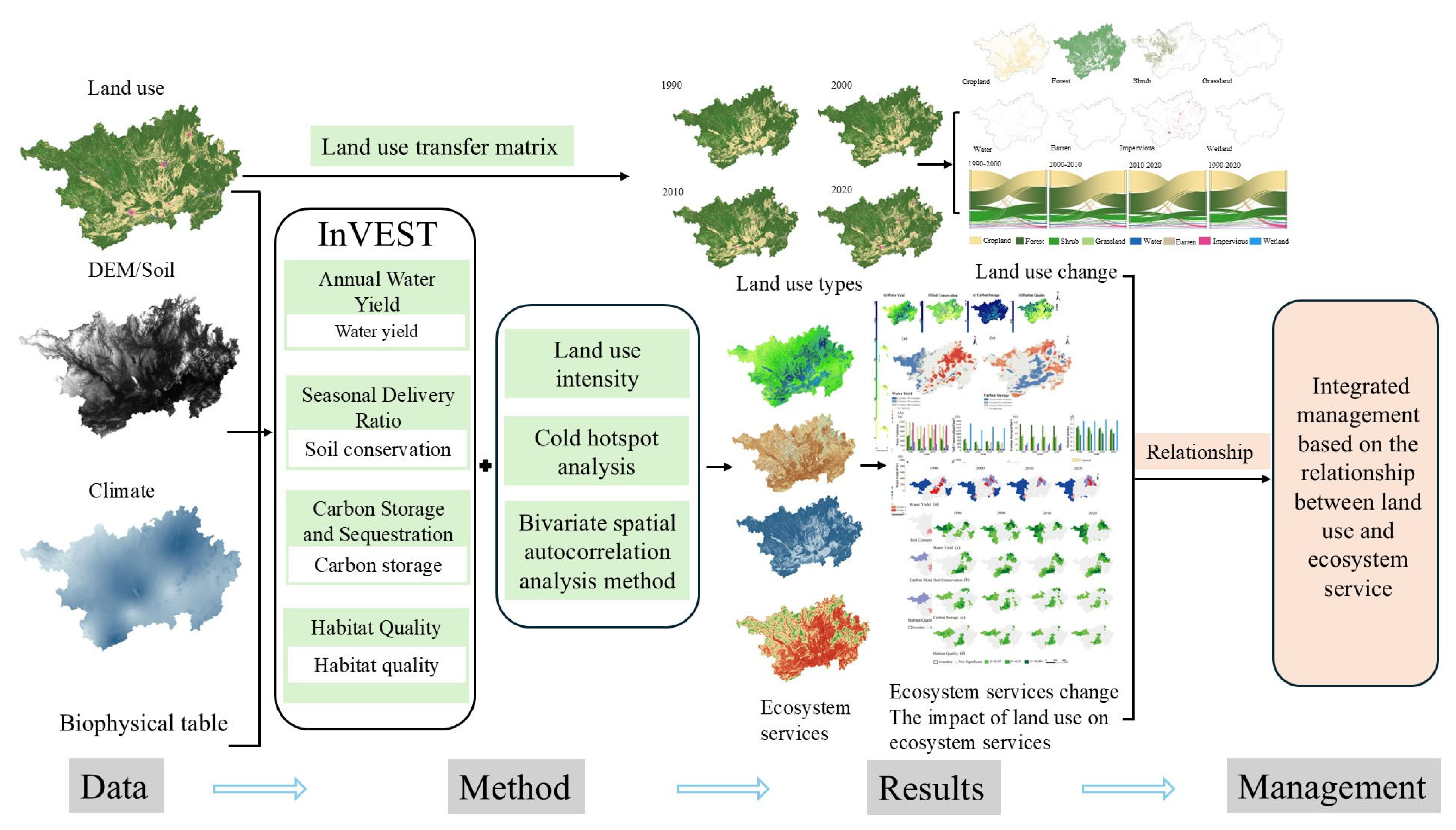
Figure 1. Analytical framework of the study.
Sustainability 17 10558 g001
Figure 2. Geographical position of the research region.
Sustainability 17 10558 g002
Figure 3. The evolution of land use patterns in the Guangxi Xijiang River Basin for the years 1990, 2000, 2010, and 2020.
Sustainability 17 10558 g003
Figure 4. Land use transitions based on transfer matrix of the study area in 1990, 2000, 2010, and 2020.
Sustainability 17 10558 g004
Figure 5. Ecosystem services functions of the Guangxi Xijiang River Basin in 1990, 2000, 2010, and 2020. Among them: (a) denotes water yield; (b) denotes soil conservation; (c) denotes carbon storage; (d) denotes habitat quality.
Sustainability 17 10558 g005
Figure 6. Characteristics of spatiotemporal distribution of four categories of ecosystem services within Guangxi’s Xijiang River Basin across 1990, 2000, 2010, and 2020. Among them: (a) represents water yield; (b) represents soil conservation; (c) represents carbon storage; (d) represents habitat quality.
Sustainability 17 10558 g006
Figure 7. Multi-year average cold and hot spots of four ecosystem services in the Guangxi Xijiang River Basin in 1990, 2000, 2010, and 2020. Among them: (a) is water yield; (b) is soil conservation; (c) is carbon storage; (d) is habitat quality.
Sustainability 17 10558 g007
Figure 8. (A) Average levels of water yield (i), soil conservation (ii), carbon storage (iii), and habitat quality (iv) for various land use types in the Guangxi Xijiang River Basin from 1990 to 2020; (B) total value of water yield (v), soil conservation (vi), and carbon storage (vii) for various land use types in the Guangxi Xijiang River Basin in 1990, 2000, 2010, and 2020.
Sustainability 17 10558 g008
Figure 9. LISA cluster distribution map of the comprehensive index of land use intensity and four ecosystem services in the Guangxi Xijiang River Basin in 1990, 2000, 2010, and 2020. Among them: (a) denotes water yield; (b) denotes soil conservation; (c) denotes carbon storage; (d) denotes habitat quality.
Sustainability 17 10558 g009
Figure 10. Spatial distribution of LISA significance levels for the integrated index of land use intensity and four ecosystem services in 1990, 2000, 2010, and 2020. Among them: (a) is water yield; (b) is soil conservation; (c) is carbon storage; (d) is habitat quality.
Sustainability 17 10558 g010
Table 1. Bivariate spatial autocorrelation between the comprehensive index of land use intensity and four ecosystem services in 1990, 2000, 2010, and 2020.
Water Yield1990 2000 2010 2020 Mean Value
Moran’s I0.53330.38800.43600.40380.44
p-value0.0010.0010.0010.001
Z-value8.86127.03957.82757.4999
Soil conservation1990200020102020Mean value
Moran’s I−0.4182−0.3811−0.3793−0.2726−0.36
p-value0.0010.0010.0010.001
Z-value−7.2727−6.7500−6.6760−5.0252
Carbon storage1990200020102020Mean value
Moran’s I−0.6276−0.6357−0.6191−0.5888−0.62
p-value0.0010.0010.0010.001
Z-value−9.5731−9.6283−9.4098−8.9514
Habitat quality1990200020102020Mean value
Moran’s I−0.4675−0.4681−0.4435−0.4399−0.45
p-value0.0010.0010.0010.001
Z-value−7.8867−7.8492−7.4754−7.4908
Disclaimer/Publisher’s Note: The statements, opinions and data contained in all publications are solely those of the individual author(s) and contributor(s) and not of MDPI and/or the editor(s). MDPI and/or the editor(s) disclaim responsibility for any injury to people or property resulting from any ideas, methods, instructions or products referred to in the content.