Appendix A
Table A1.
Spatial Autocorrelation Analysis of All Explanatory Variables.
Table A1.
Spatial Autocorrelation Analysis of All Explanatory Variables.
| | Moran’s I | R2 | Z Score | p Value |
|---|
| TPBTA1000 | 0.746093 | 0.000080 | 83.574324 | 0.000000 |
| TPBTA10000 | 0.502461 | 0.000079 | 56.411084 | 0.000000 |
| NQPDA1000 | 0.918994 | 0.000080 | 102.923865 | 0.000000 |
| NQPDA10000 | 0.867269 | 0.000080 | 97.107082 | 0.000000 |
| Bus Stop | 0.991140 | 0.000080 | 110.988637 | 0.000000 |
| Metro Station | 0.994295 | 0.000080 | 111.327239 | 0.000000 |
| Building Density | 0.66958 | 0.000080 | 74.981112 | 0.000000 |
| Floor Area Ratio | 0.756198 | 0.000080 | 84.685642 | 0.000000 |
| Road Density | 0.627165 | 0.000080 | 70.241239 | 0.000000 |
| Average Housing Price | 0.479179 | 0.000080 | 53.701269 | 0.000000 |
| POI Density | 0.712069 | 0.000080 | 79.895480 | 0.000000 |
| POI Mix Index | 0.727543 | 0.000080 | 81.462662 | 0.000000 |
| Shopping & Retail | 0.861887 | 0.000079 | 96.808261 | 0.000000 |
| Landscape | 0.946578 | 0.000079 | 106.382142 | 0.000000 |
| Catering | 0.897002 | 0.000079 | 100.743711 | 0.000000 |
| Leisure & Entertainment | 0.958889 | 0.000080 | 107.467371 | 0.000000 |
| Hotel & Accommodation | 0.933813 | 0.000079 | 104.909135 | 0.000000 |
| Healthcare | 0.938535 | 0.000080 | 105.198327 | 0.000000 |
| Life Service | 0.930476 | 0.000080 | 104.303840 | 0.000000 |
| Commercial & Residential | 0.971676 | 0.000080 | 108.964231 | 0.000000 |
| Science & Education | 0.955393 | 0.000080 | 107.039829 | 0.000000 |
| Corporate & Enterprise | 0.956727 | 0.000080 | 107.187181 | 0.000000 |
This table presents the global spatial autocorrelation analysis results for each explanatory variable. The Moran’s I values for all variables are positive with p-values less than 0.01, indicating statistically significant spatial clustering. The Moran’s I ranges from 0.479 (average housing price) to 0.994 (subway stations), demonstrating moderate to very strong spatial autocorrelation.
Table A2.
OLS Analysis of All Influencing Factors on the Peak Season (1 January).
Table A2.
OLS Analysis of All Influencing Factors on the Peak Season (1 January).
| Variable | Coefficient [a] | StdError | Probability [b] | VIF [c] |
|---|
| Intercept | 680.617936 | 234.465781 | 0.003718 * | -------- |
| NQPDA1000 | −1640.452700 | 679.580788 | 0.015796 * | 8.898169 |
| TPBTA1000 | 68.790793 | 47.885670 | 0.150906 | 5.323968 |
| NQPDA10000 | 73.055809 | 16.266724 | 0.000010 * | 7.800938 |
| TPBTA10000 | 7.840457 | 1.585912 | 0.000001 * | 1.602675 |
| Road Network Density | 134,744.50816 | 15,002.613208 | 0.000000 * | 3.566915 |
| Distance to Bus Depot/Terminal | −0.164531 | 0.068907 | 0.016967 * | 3.072622 |
| Distance to Metro Station | 0.032066 | 0.055121 | 0.560770 | 3.418771 |
| Floor Area Ratio | 2055.902227 | 198.525817 | 0.000000 * | 3.346409 |
| Building Density | −765.478870 | 579.858628 | 0.000000 * | 1.002461 |
| Average Housing Price | 0.166603 | 0.020904 | 0.000000 * | 1.789764 |
| POI Density | 7.568737 | 0.398009 | 0.000000 * | 7.329613 |
| POI Mix | 3052.703164 | 166.320978 | 0.000000 * | 3.372136 |
| Shopping & Retail | −1.154325 | 0.938806 | 0.218908 | 6.016032 |
| Landscape & Attractions | −46.596555 | 29.345276 | 0.112379 | 1.886030 |
| Catering | 23.561568 | 4.181377 | 0.000000 * | 5.843977 |
| Leisure & Entertainment | 83.481735 | 27.540555 | 0.002458 * | 6.227914 |
| Hotel & Accommodation | 61.855724 | 5.035808 | 0.000000 * | 3.890451 |
| Medical & Insurance | 14.339805 | 5.570346 | 0.010058 * | 6.510724 |
| Life Services | −20.221038 | 2.733236 | 0.000000 * | 10.065604 |
| Commercial & Residential | 1.355120 | 12.070152 | 0.910596 | 5.473145 |
| Science, Education & Culture | 7.142377 | 6.537603 | 0.274645 | 5.086368 |
| Corporations & Enterprises | −60.968105 | 4.632331 | 0.000000 * | 4.009531 |
This table presents the global OLS model regression results for all explanatory variables during the peak season. The asterisk (*) next to the probability values (Probability [b]) indicates statistical significance (p < 0.05). The “Coefficient” indicates the direction and strength of the influence of the independent variables on the dependent variable. Variables marked with [b] are statistically significant at the 0.05 level, such as road network density, floor area ratio, and POI density, which exhibit significant positive effects on peak-season demand. The notation [c] indicates the presence of evident multicollinearity issues in the model, which will be addressed in subsequent steps by removing collinear explanatory variables for optimization.
Table A3.
Data of the OLS Model Pertaining to the Peak Season (1 January).
Table A3.
Data of the OLS Model Pertaining to the Peak Season (1 January).
| AIC | AICc | R2 | R2 Adjusted | F-Stat | F-Prob |
|---|
| 127,151.71328200000 | 127,151.95109300000 | 0.68655142178 | 0.68531931259 | 557.21637880600 | 0.00000000000 |
The OLS regression results demonstrate that the model exhibits good explanatory power on the peak-season data. The adjusted R2 of 0.685 indicates that the independent variables explain 68.5% of the variance in the dependent variable. The F-statistic is highly significant at the 0.01 level (p < 0.01), confirming the overall validity of the model.
Table A4.
OLS Model Results After Multicollinearity Remediation for the Peak Season (1 January).
Table A4.
OLS Model Results After Multicollinearity Remediation for the Peak Season (1 January).
| Variable | Coefficient [a] | StdError | Probability [b] | VIF [c] |
|---|
| Intercept | 449.822781 | 189.705340 | 0.017746 * | -------- |
| NQPDA10000 | 45.428387 | 11.674707 | 0.000110 * | 3.937862 |
| TPBTA10000 | 8.391897 | 1.557365 | 0.000000 * | 1.514572 |
| Road Network Density | 122,145.80946 | 11,436.977546 | 0.000000 * | 2.031436 |
| Distance to Bus Depot/Terminal | −0.167484 | 0.051928 | 0.001281 * | 1.710024 |
| Floor Area Ratio | 1999.814212 | 199.036540 | 0.000000 * | 3.296343 |
| Average Housing Price | 0.175988 | 0.020680 | 0.000000 * | 1.716579 |
| POI Density | 7.215932 | 0.253213 | 0.000000 * | 2.907294 |
| POI Mix | 3105.111577 | 162.739885 | 0.000000 * | 3.163886 |
| Hotel & Accommodation | 72.541993 | 3.922842 | 0.000000 * | 2.313583 |
| Corporations & Enterprises | −66.063048 | 3.954790 | 0.000000 * | 2.863935 |
After variable screening, the VIF values of all retained variables were below 5, indicating that multicollinearity issues had been mitigated. The asterisk (*) next to the probability values (Probability [b]) indicates statistical significance (
p < 0.05). For building density, although its VIF value was acceptable, it was ultimately excluded from the final modeling due to the following considerations: its coefficient sign was inconsistent with theoretical expectations, and its inclusion might interfere with the local parameter estimation of other variables with greater spatial stability. Except for the intercept term, all variables had a significant effect on the dependent variable at the 0.05 level (
p < 0.05). The model was subsequently used for GWR analysis, with specific results presented in
Figure 15 in the main text.
Table A5.
OLS Model Data after Removing Multicollinearity (1 January).
Table A5.
OLS Model Data after Removing Multicollinearity (1 January).
| AIC | AICc | R2 | Adj. R2 | F-Stat | F-Prob |
|---|
| 127,151.71328200000 | 127,151.95109300000 | 0.68655142178 | 0.68531931259 | 557.21637880600 | 0.00000000000 |
The diagnostic metrics of the OLS model indicate that the model is overall significant and demonstrates a good fit (Adj. R2 = 0.685, F-test p-value < 0.01). These results provide a reliable baseline model for the subsequent Geographically Weighted Regression (GWR) analysis. The AICc value (127,151.713) will be used for comparing the goodness-of-fit with the GWR model.
Table A6.
OLS Analysis of All Influencing Factors for the off-Season (15 March).
Table A6.
OLS Analysis of All Influencing Factors for the off-Season (15 March).
| Variable | Coefficient [a] | StdError | Probability [b] | VIF [c] |
|---|
| Intercept | 716.223813 | 258.344758 | 0.005583 * | -------- |
| NQPDA1000 | −2155.505639 | 748.792143 | 0.004014 * | 8.898169 |
| TPBTA1000 | 96.505870 | 52.762547 | 0.067439 | 5.323968 |
| NQPDA10000 | 70.867598 | 17.923396 | 0.000086 * | 7.800938 |
| TPBTA10000 | 9.092760 | 1.747428 | 0.000000 * | 1.602675 |
| Road Network Density | 166,614.92549 | 16,530.542193 | 0.000000 * | 3.566915 |
| Distance to Bus Depot/Terminal | −0.183259 | 0.075925 | 0.015805 * | 3.072622 |
| Distance to Metro Station | 0.032747 | 0.060735 | 0.589794 | 3.418771 |
| Floor Area Ratio | 2307.161466 | 218.744517 | 0.000000 * | 3.346409 |
| Building Density | −226.718486 | 638.913861 | 0.722728 | 1.002461 |
| Average Housing Price | 0.122858 | 0.023033 | 0.000000 * | 1.789764 |
| POI Density | 8.950145 | 0.438544 | 0.000000 * | 7.329613 |
| POI Mix | 3357.537913 | 183.259803 | 0.000000 * | 3.372136 |
| Shopping & Retail | 0.539975 | 1.034418 | 0.601694 | 6.016032 |
| Landscape & Attractions | −237.819059 | 32.333922 | 0.000000 * | 1.886030 |
| Catering | 16.584760 | 4.607226 | 0.000335 * | 5.843977 |
| Leisure & Entertainment | 52.524340 | 30.345401 | 0.083529 | 6.227914 |
| Hotel & Accommodation | 32.189913 | 5.548676 | 0.000000 * | 3.890451 |
| Medical & Insurance | 23.844233 | 6.137653 | 0.000113 * | 6.510724 |
| Life Services | −23.657281 | 3.011600 | 0.000000 * | 10.065604 |
| Commercial & Residential | 17.519495 | 13.299427 | 0.187791 | 5.473145 |
| Science, Education & Culture | 50.970112 | 7.203420 | 0.000000 * | 5.086368 |
| Corporations & Enterprises | −62.065938 | 5.104107 | 0.000000 * | 4.009531 |
This table presents the global OLS model regression results for all explanatory variables during the off-season (15 March). The asterisk next to the probability values indicates statistical significance (p < 0.05). The “Coefficient” indicates the direction and strength of the influence of the independent variables on the dependent variable. Variables with statistically significant probability values have a significant impact on off-season demand. The VIF value is used to diagnose multicollinearity; the high VIF values of some variables indicate evident multicollinearity issues in the model, which will be addressed in subsequent steps by removing collinear explanatory variables for optimization.
Table A7.
Data of the OLS Model Pertaining to the off-Season (15 March).
Table A7.
Data of the OLS Model Pertaining to the off-Season (15 March).
| Diag_Name | Diag_Value |
|---|
| AIC | 128,388.79792700000 |
| AICc | 128,389.01871700000 |
| R2 | 0.68859973334 |
| AdjR2 | 0.68742482273 |
| F-Stat | 586.08691299500 |
| F-Prob | 0.00000000000 |
The OLS regression results indicate that the model demonstrates good explanatory power on the off-season data. The adjusted R2 value of 0.687 shows that the independent variables explain 68.7% of the variance in the dependent variable. The F-statistic is highly significant at the 0.01 level (p < 0.01), confirming the overall validity of the model.
Table A8.
OLS Model Results After Multicollinearity Remediation for the off-Season (15 March).
Table A8.
OLS Model Results After Multicollinearity Remediation for the off-Season (15 March).
| Variable | Coefficient [a] | StdError | Probability [b] | VIF [c] |
|---|
| Intercept | 797.729379 | 191.325393 | 0.000036 * | -------- |
| TPBTA10000 | 11.672668 | 1.570638 | 0.000000 * | 1.277782 |
| Road Network Density | 164,122.64045 | 11,842.119305 | 0.000000 * | 1.806488 |
| Average Housing Price | −0.228592 | 0.054214 | 0.000030 * | 1.546067 |
| Distance to Bus Depot/Terminal | 2300.754568 | 215.877468 | 0.000000 * | 3.216451 |
| Floor Area Ratio | 0.124420 | 0.022918 | 0.000000 * | 1.748728 |
| POI Density | 8.632011 | 0.280830 | 0.000000 * | 2.966205 |
| POI Mix | 3330.238611 | 180.143074 | 0.000000 * | 3.215611 |
| Landscape & Attractions | −193.733922 | 29.681137 | 0.000000 * | 1.568378 |
| Hotel & Accommodation | 35.359382 | 4.827363 | 0.000000 * | 2.906022 |
| Science, Education & Culture | 65.382243 | 5.632403 | 0.000000 * | 3.068849 |
| Corporations & Enterprises | −67.469280 | 4.483835 | 0.000000 * | 3.053592 |
This table presents the final set of variables selected for the Geographically Weighted Regression analysis. After the screening process, all retained variables exhibit acceptable Variance Inflation Factor values (<5) and statistically significant p-values (p < 0.01). These results confirm the overall robustness of the model and indicate that multicollinearity issues have been effectively resolved, thereby satisfying the prerequisite conditions for conducting GWR analysis.
Table A9.
OLS Model Data after Removing Multicollinearity (15 March).
Table A9.
OLS Model Data after Removing Multicollinearity (15 March).
| Diag_Name | Diag_Value |
|---|
| AIC | 128,460.27214200000 |
| AICc | 128,460.32926700000 |
| R2 | 0.68381014151 |
| AdjR2 | 0.68326447341 |
| F-Stat | 1253.16130191000 |
| F-Prob | 0.00000000000 |
The model diagnostic metrics indicate that, after controlling for multicollinearity, the independent variables explain approximately 68.3% of the variance in the dependent variable (Adjusted R2 = 0.683), and the model is highly significant overall (p < 0.001). The AIC and AICc values will serve as benchmarks for subsequent comparisons of goodness-of-fit with local models such as GWR.
Table A10.
Spatial Autocorrelation Analysis (Global Moran’s I) of GWR Model Coefficients for the Peak Season (1 January).
Table A10.
Spatial Autocorrelation Analysis (Global Moran’s I) of GWR Model Coefficients for the Peak Season (1 January).
| Variable Description | Moran’s I | z-Score | p-Value | Spatial Pattern Judgment |
|---|
| POI Functional Mix Index | 0.993324 | 111.533 | <0.001 | Highly Significant Clustering |
| POI Density | 0.985401 | 110.666 | <0.001 | Highly Significant Clustering |
| Road Betweenness (Vehicular) | 0.980215 | 110.054 | <0.001 | Highly Significant Clustering |
| Road Network Density | 0.994259 | 111.643 | <0.001 | Highly Significant Clustering |
| Housing Price | 0.988510 | 110.990 | <0.001 | Highly Significant Clustering |
| Accessibility to Bus Stops | 0.997275 | 111.999 | <0.001 | Highly Significant Clustering |
| Corporate Density | 0.986078 | 110.722 | <0.001 | Highly Significant Clustering |
| Hotel Density | 0.972212 | 109.167 | <0.001 | Highly Significant Clustering |
| Floor Area Ratio (FAR) | 0.997287 | 111.981 | <0.001 | Highly Significant Clustering |
This table presents the Global Moran’s I analysis results of the regression coefficients for each driving factor in the peak-season GWR model. All coefficients exhibit a highly significant positive spatial correlation at the level of p < 0.001, indicating that their influence intensity demonstrates high spatial clustering and regularity, rather than a random distribution.
Table A11.
Spatial Autocorrelation Analysis (Global Moran’s I) of GWR Model Coefficients for the Off-Season (15 March).
Table A11.
Spatial Autocorrelation Analysis (Global Moran’s I) of GWR Model Coefficients for the Off-Season (15 March).
| Variable Description | Moran’s I | Z-Score | p-Value | Spatial Pattern Judgment |
|---|
| Bus Stop Accessibility | 1.001507 | 112.501 | <0.001 | Highly Significant Clustering |
| Road Network Density | 0.999001 | 112.170 | <0.001 | Highly Significant Clustering |
| Floor Area Ratio | 0.998528 | 112.133 | <0.001 | Highly Significant Clustering |
| Road Betweenness | 0.985473 | 110.643 | <0.001 | Highly Significant Clustering |
| Housing Price | 0.985821 | 110.693 | <0.001 | Highly Significant Clustering |
| POI Density | 0.982313 | 110.315 | <0.001 | Highly Significant Clustering |
| Sci-Edu Density | 0.974207 | 109.417 | <0.001 | Highly Significant Clustering |
| Hotel Density | 0.961187 | 107.942 | <0.001 | Highly Significant Clustering |
| Scenic Spot Distribution | 0.952843 | 107.278 | <0.001 | Highly Significant Clustering |
| Corporate Density | 0.991270 | 111.302 | <0.001 | Highly Significant Clustering |
| POI Functional Mix Index | 0.992730 | 111.460 | <0.001 | Highly Significant Clustering |
This table presents the spatial autocorrelation analysis results of the regression coefficients for each variable in the off-season GWR model after controlling for multicollinearity. Similarly to the peak season, all coefficients exhibit highly significant spatial clustering, revealing that the off-season driving mechanisms also possess strong spatial dependence characteristics.
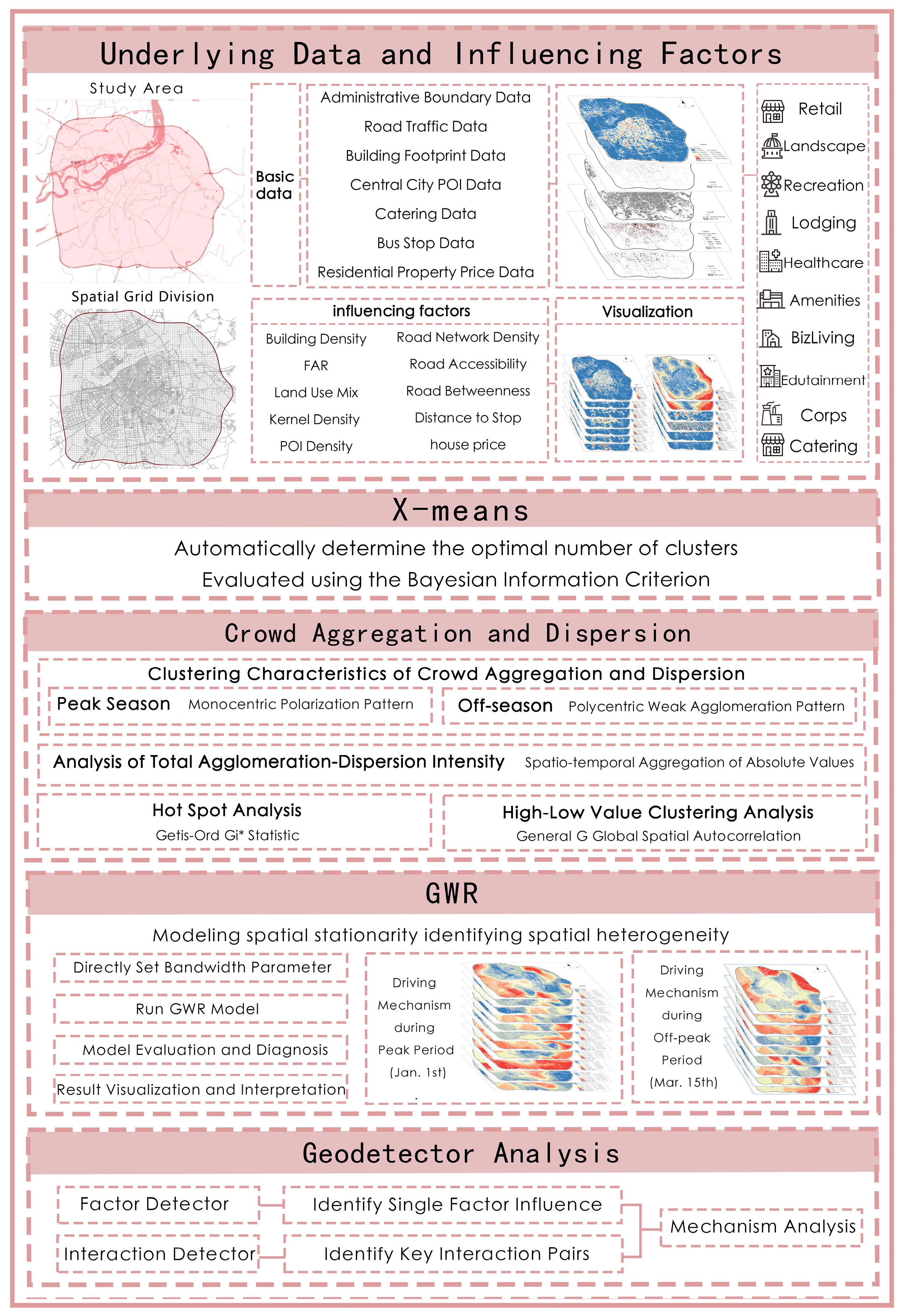
Figure 1.
Article Framework Diagram. This figure illustrates the technical framework for analyzing crowd aggregation and dispersion. In this chart, solid arrows indicate the main analytical procedure or strong direct relationships; dashed arrows represent supportive data flows, interpretive relationships, and model inputs.
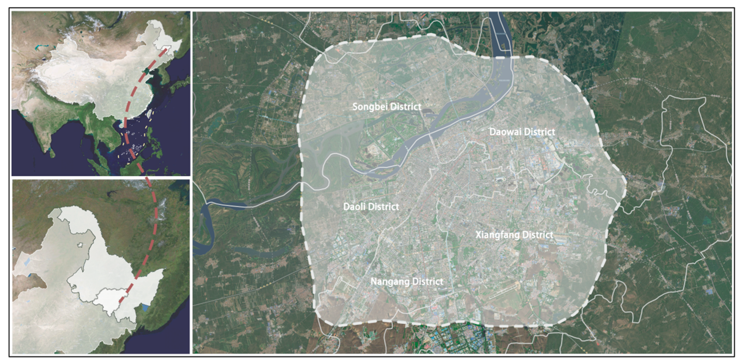
Figure 2.
The figure depicts the study area located within the Fourth Ring Road of Harbin City, Heilongjiang Province, China.
Figure 2.
The figure depicts the study area located within the Fourth Ring Road of Harbin City, Heilongjiang Province, China.
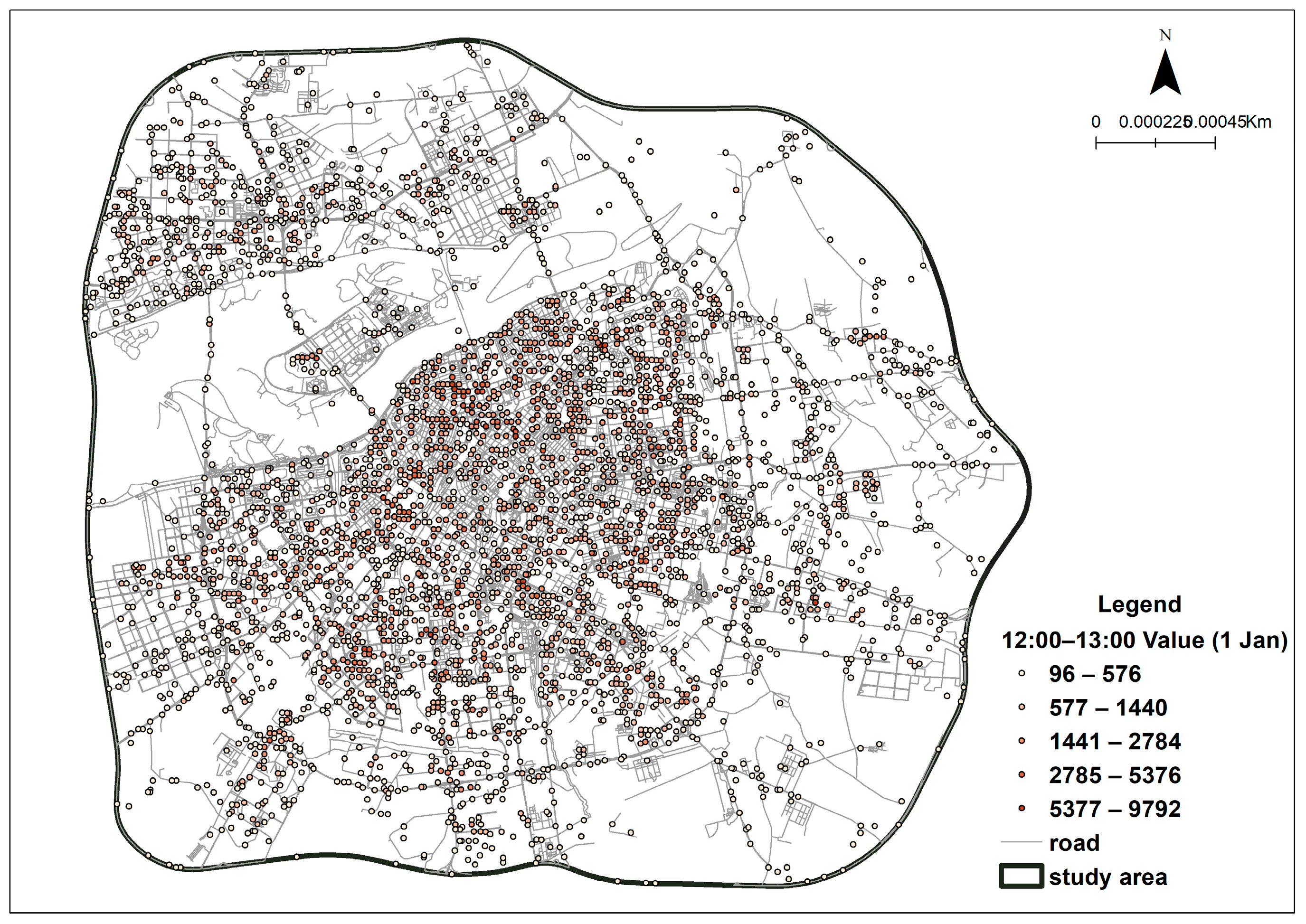
Figure 3.
This figure presents the initial heatmap data for the time period 12:00–13:00 on 1 January 2025. The color intensity at each point corresponds to the magnitude of the heatmap value.
Figure 3.
This figure presents the initial heatmap data for the time period 12:00–13:00 on 1 January 2025. The color intensity at each point corresponds to the magnitude of the heatmap value.
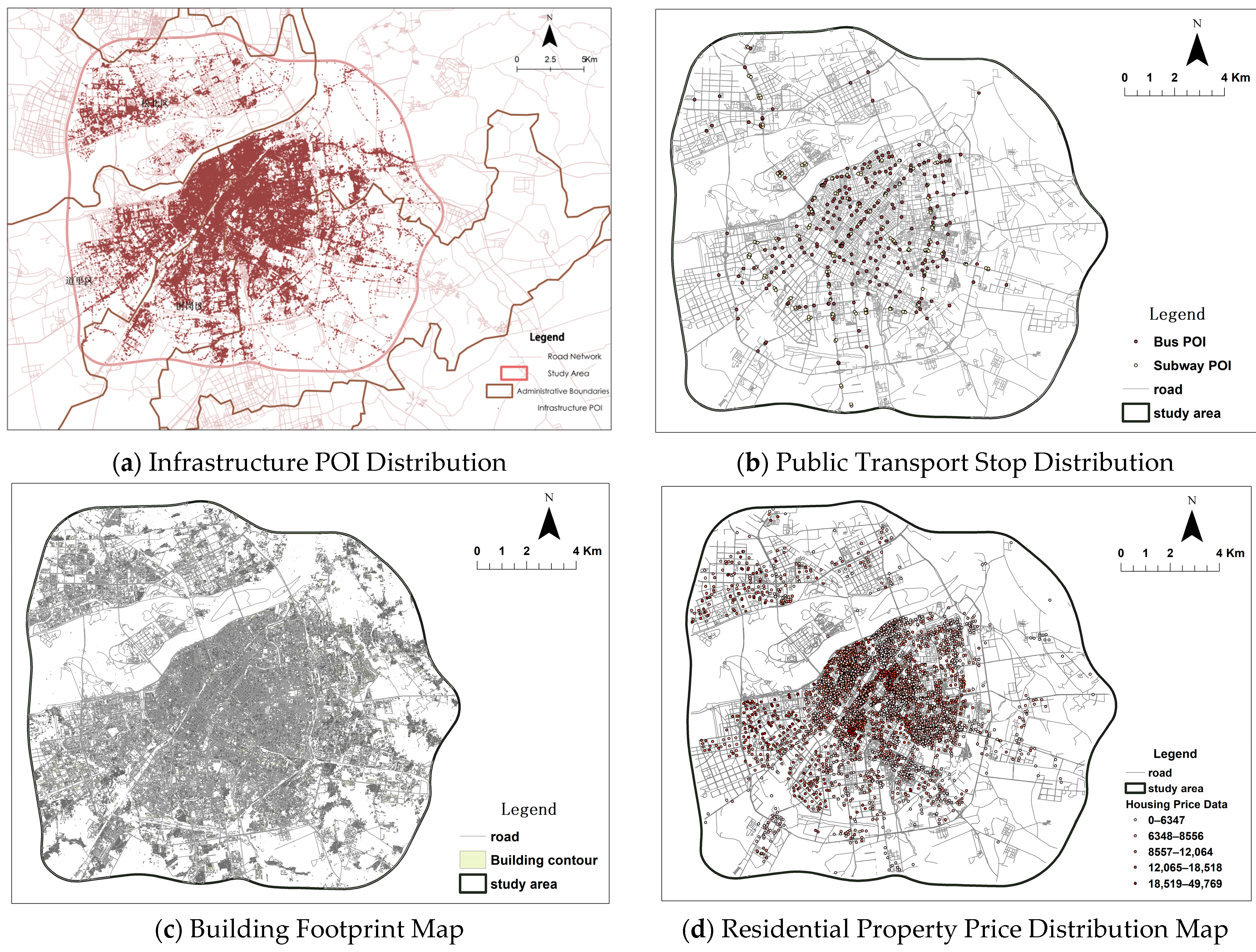
Figure 4.
Spatial distribution of the four key types of built environment and socioeconomic data used in this study: (a) Points of Interest (POI), (b) public transport stops, (c) building footprints, and (d) residential property prices.
Figure 4.
Spatial distribution of the four key types of built environment and socioeconomic data used in this study: (a) Points of Interest (POI), (b) public transport stops, (c) building footprints, and (d) residential property prices.
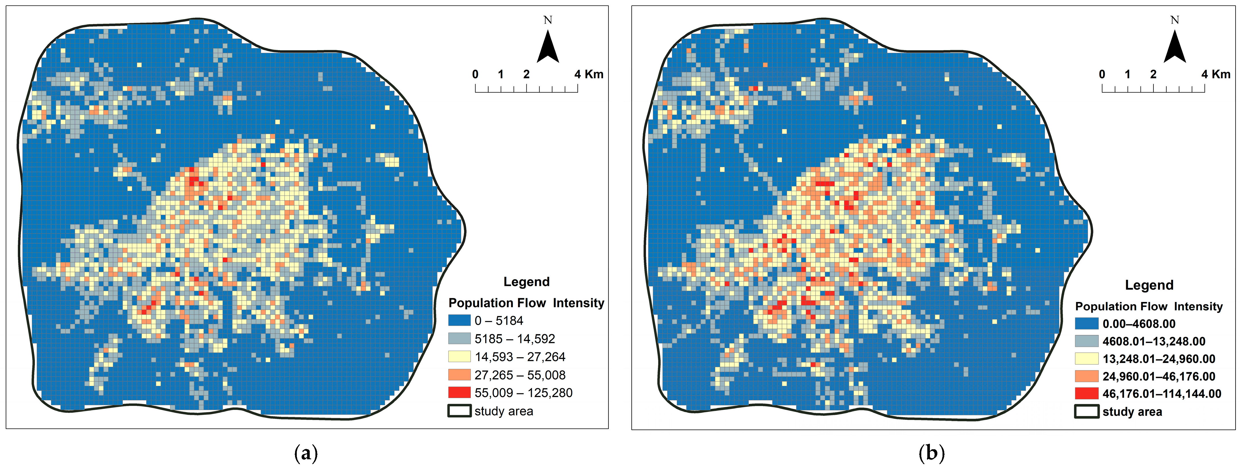
Figure 5.
Total Intensity of Population Aggregation and Dispersion: (a) Peak Season vs. (b) Off-Season.
Figure 5.
Total Intensity of Population Aggregation and Dispersion: (a) Peak Season vs. (b) Off-Season.
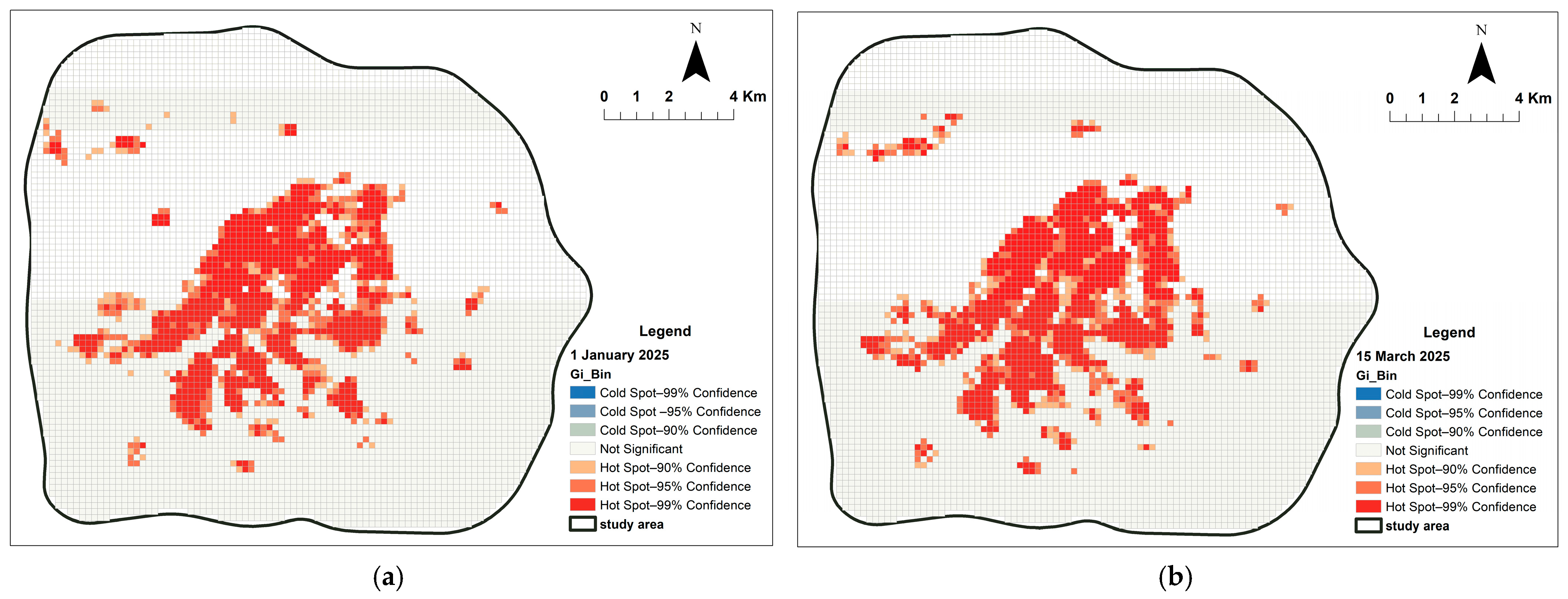
Figure 6.
This figure shows the hot spot and cold spot analysis of population aggregation/dispersion intensity for both seasons, with the primary difference located near Taiyang Island. (a) peak season. (b) off-season.
Figure 6.
This figure shows the hot spot and cold spot analysis of population aggregation/dispersion intensity for both seasons, with the primary difference located near Taiyang Island. (a) peak season. (b) off-season.
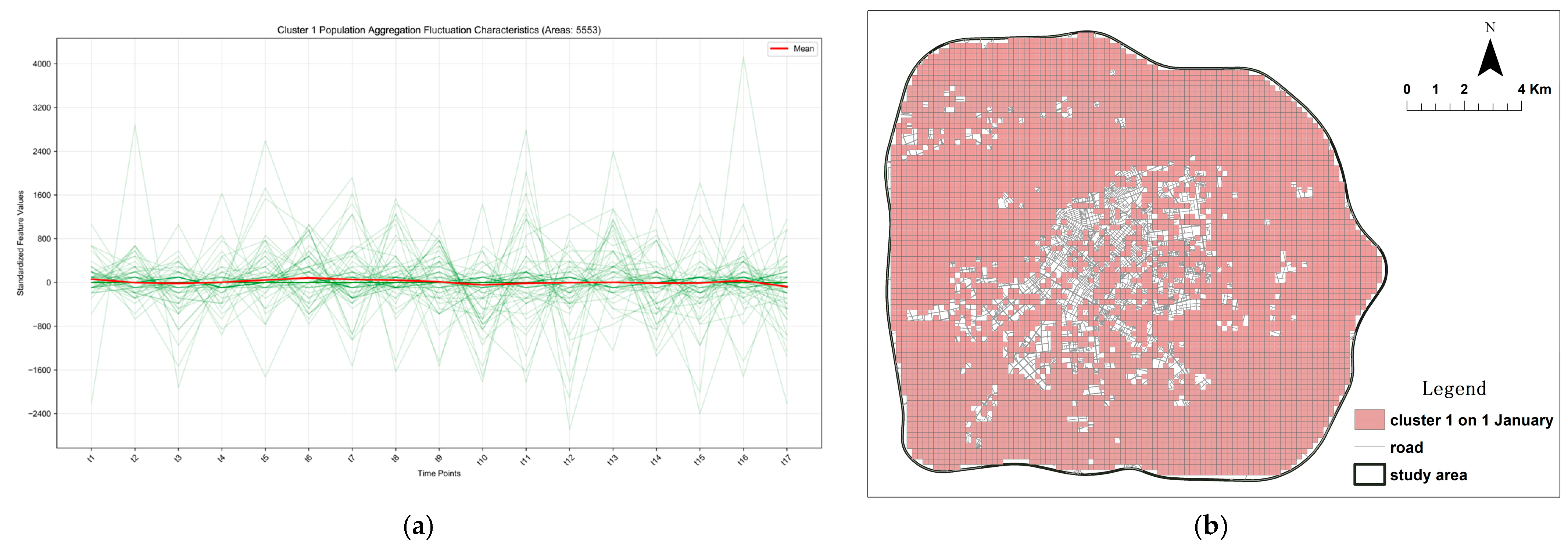
Figure 7.
Cluster Characteristics and Spatial Distribution of Peak-season Population Aggregation/Dispersion Category 1 Based on Clustering Analysis. The green lines depict the temporal variation in standardized aggregation values across all regions. (a) Spatio-temporal fluctuation characteristics of Cluster 1. (b) Spatial distribution pattern of Cluster 1.
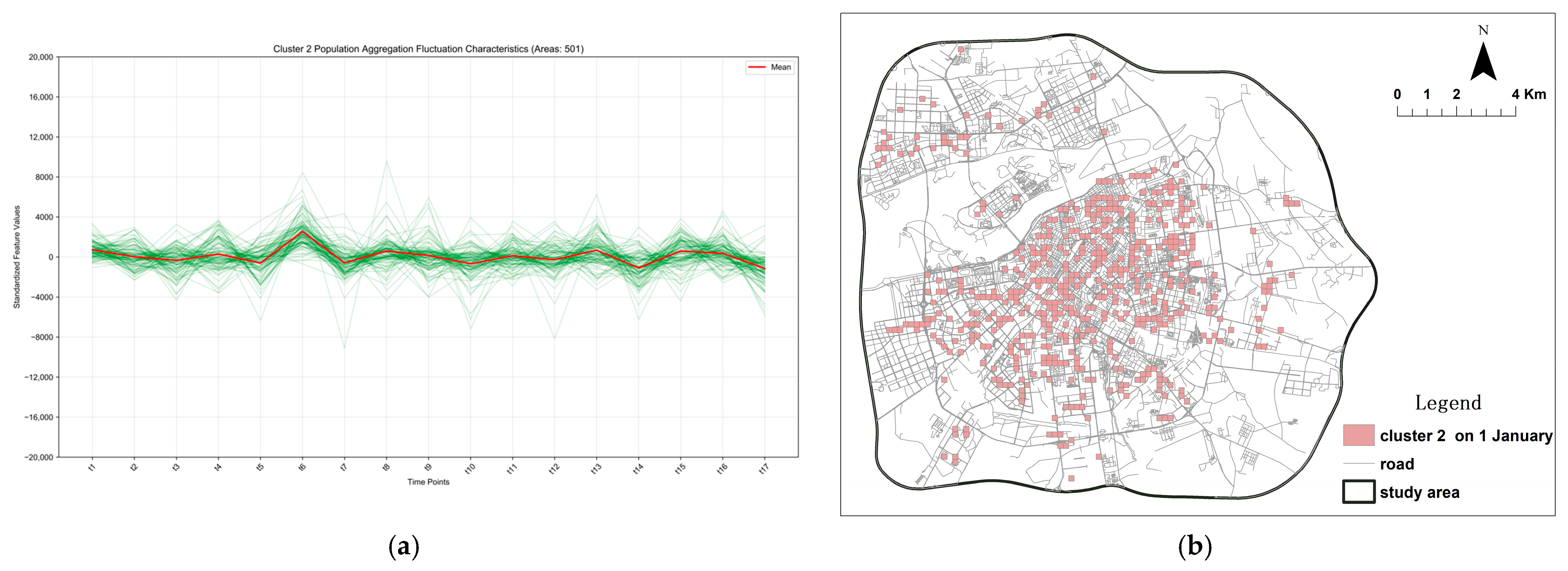
Figure 8.
This is a figure, illustrates the cluster characteristics and spatial distribution of population aggregation/dispersion Category 2 during the peak season, which functions as a passenger flow distribution hub for tourist attractions and commercial districts. The green lines depict the temporal variation in standardized aggregation values across all regions. (a) Spatio-temporal fluctuation characteristics of Cluster 2. (b) Spatial distribution pattern of Cluster 2.
Figure 9.
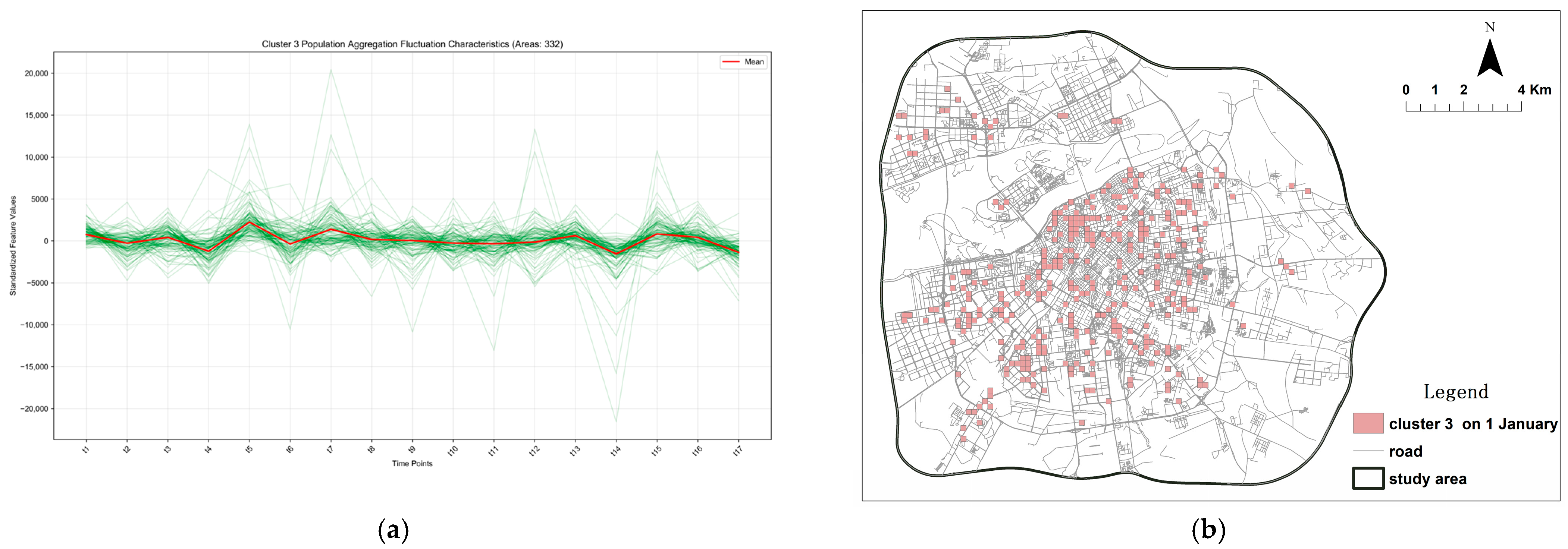
Cluster characteristics and spatial distribution of population aggregation/dispersion Category 3 during the peak season, exhibiting a typical consumption-destination pattern. The green lines depict the temporal variation in standardized aggregation values across all regions. (a) Spatio-temporal fluctuation characteristics of Cluster 3. (b) Spatial distribution pattern of Cluster 3.
Figure 10.
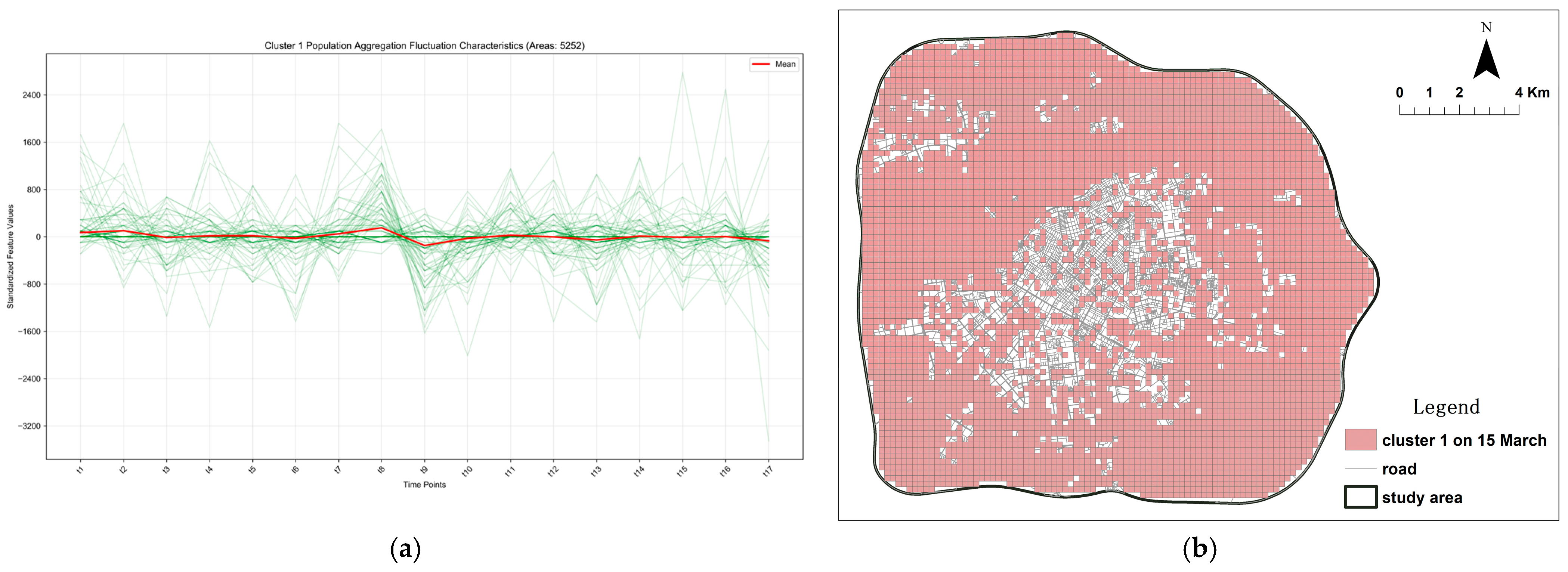
Cluster characteristics and spatial distribution of population aggregation/dispersion Category 1 during the off-season, exhibiting a pattern dominated by local commuting with both stability and pulsating characteristics. The green lines depict the temporal variation in standardized aggregation values across all regions. (a) Spatio-temporal fluctuation characteristics of Cluster 1. (b) Spatial distribution pattern of Cluster 1.
Figure 11.
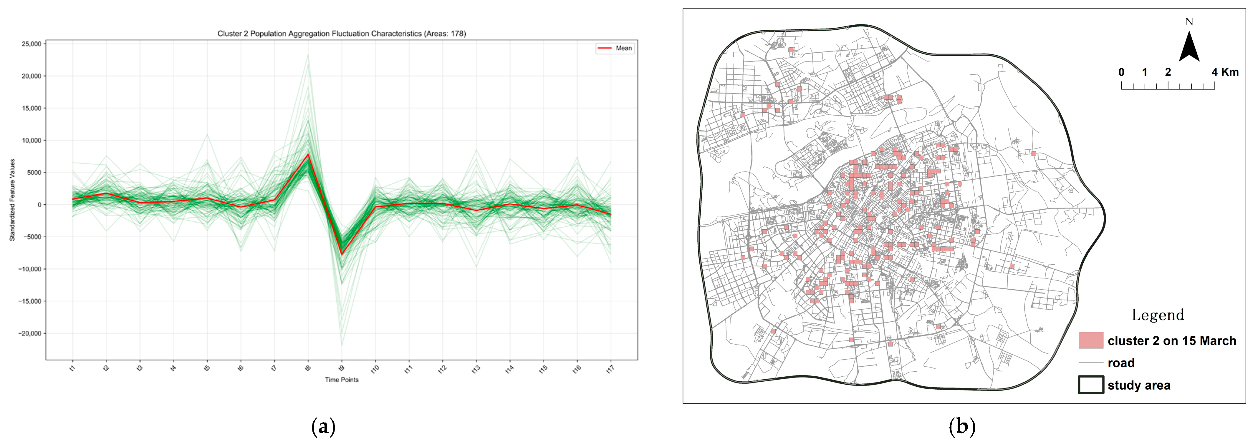
Cluster characteristics and spatial distribution of population aggregation/dispersion Category 2 during the off-season, exhibiting a short-term pulse pattern. The green lines depict the temporal variation in standardized aggregation values across all regions. (a) Spatio-temporal fluctuation characteristics of Cluster 2. (b) Spatial distribution pattern of Cluster 2.
Figure 12.
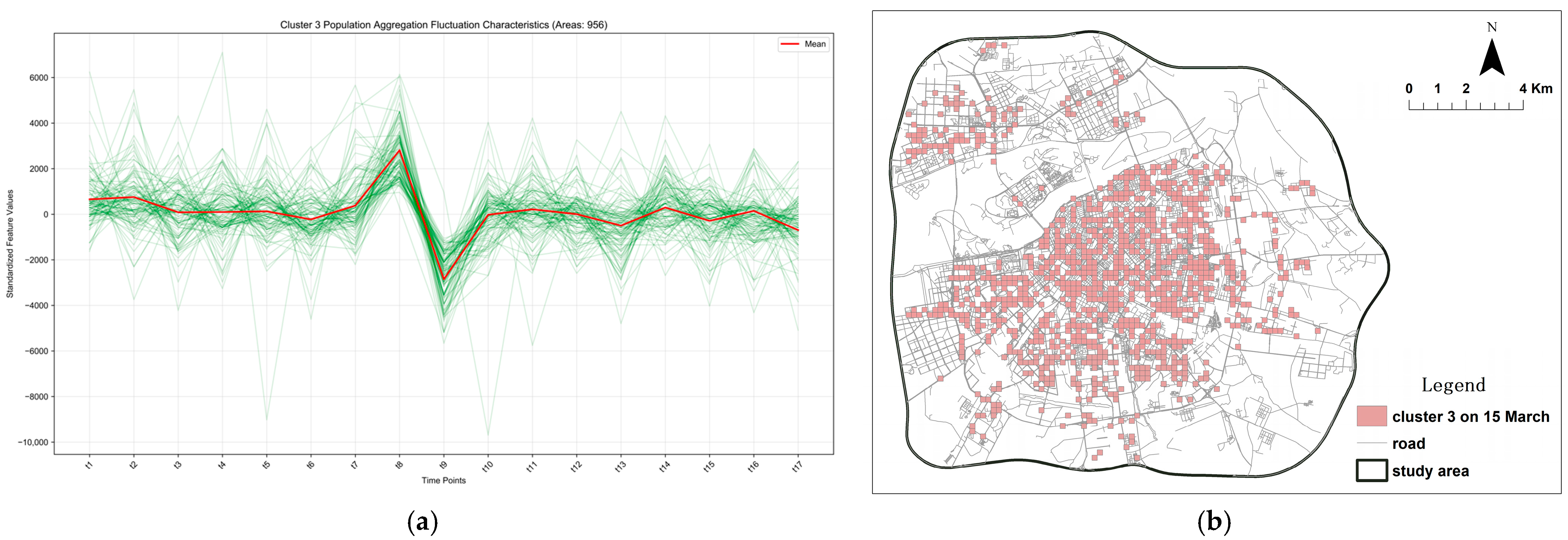
Cluster characteristics and spatial distribution of population aggregation/dispersion Category 3 during the off-season, exhibiting a resilient spatial pattern supported by the integration of commercial and residential functions. The green lines depict the temporal variation in standardized aggregation values across all regions. (a) Spatio-temporal fluctuation characteristics of Cluster 3. (b) Spatial distribution pattern of Cluster 3.
Figure 13.
Comparison of cluster characteristics for population activity during peak and off-seasons. The peak season exhibits an “area-wide fluctuation” pattern with dispersed and highly heterogeneous population activity, while the off-season shows concentration around midday fluctuations, presenting a more predictable urban operational rhythm. (a) Peak season. (b) Off-season.
Figure 14.
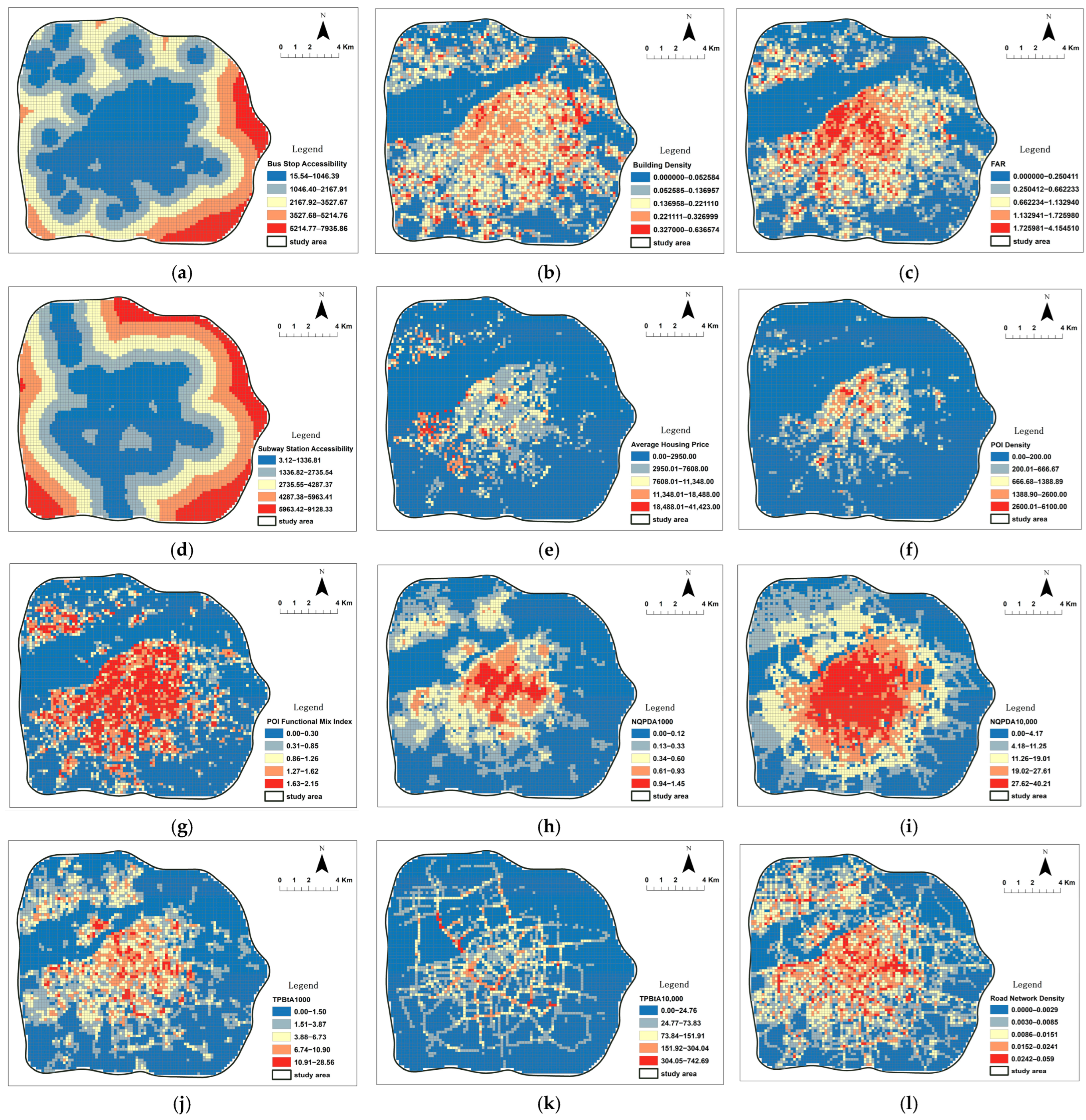
Spatial distribution of all key explanatory variables selected for this study. (a) Bus Stop Accessibility. (b) Building Density. (c) FAR. (d) Subway Station Accessibility. (e) Average Housing Price. (f) POI Density. (g) POI Functional Mix Index. (h) NPQDA Distribution at 1000 m Scale. (i) NPQDA Distribution at 10,000 m Scale. (j) TPBTA Distribution at 1000 m Scale. (k) TPBTA Distribution at 10,000m Scale. (l) Road Network Density.
Figure 15.
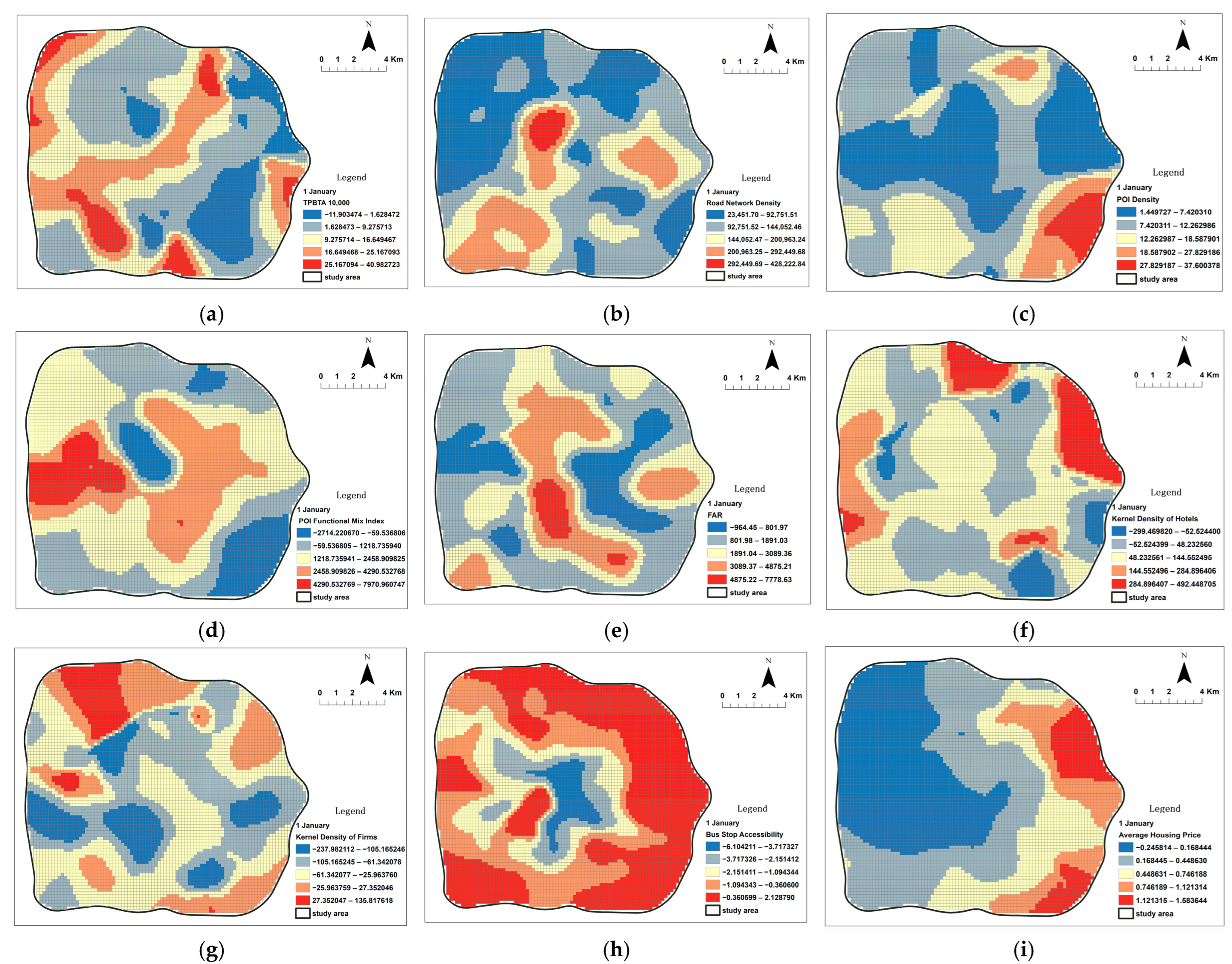
Spatial distribution of the local estimated coefficients for influencing factors of population aggregation/dispersion intensity during the peak season in Harbin. (a) TPBTA Distribution at 10,000 m Scale. (b) Road Network Density. (c) POI Density. (d) POI Functional Mix Index. (e) FAR. (f) Kernel Density of Hotels. (g) Kernel Density of Firms. (h) Bus Stop Accessibility. (i) Average Housing Price.
Figure 16.
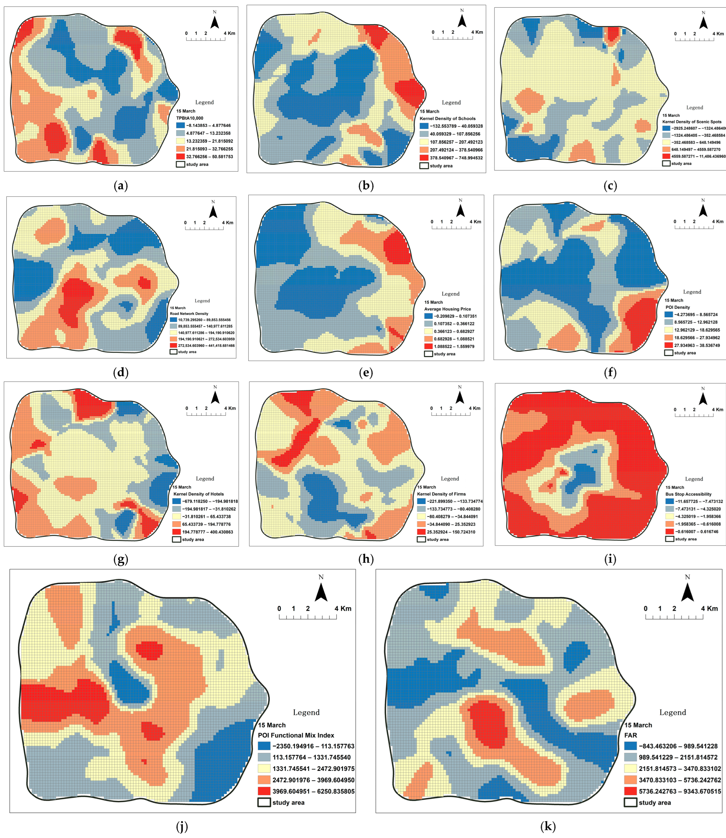
Presents the coefficient maps of explanatory variables from the off-season GWR model for Harbin. The operational mechanisms revealed in these maps contrast with those observed during the peak season, demonstrating the urban system’s off-season resilience—achieved through functional transformation and demand rebalancing—during periods of low demand. (a) TPBTA Distribution at 10,000 m Scale. (b) Kernel Density of Schools. (c) Kernel Density of Scenic Spots. (d) Road Network Density. (e) Average Housing Price. (f) POI Density. (g) Kernel Density of Hotels. (h) Kernel Density of Firms. (i) Bus Stop Accessibility. (j) POI Functional Mix Index. (k) FAR.
Figure 17.
Spatial Clustering Analysis Results of Population Activity on Peak-Season Workdays.The green lines depict the temporal variation in standardized aggregation values across all regions. (a) Cluster 0. (b) Cluster 1.
Figure 17.
Spatial Clustering Analysis Results of Population Activity on Peak-Season Workdays.The green lines depict the temporal variation in standardized aggregation values across all regions. (a) Cluster 0. (b) Cluster 1.
Figure 18.
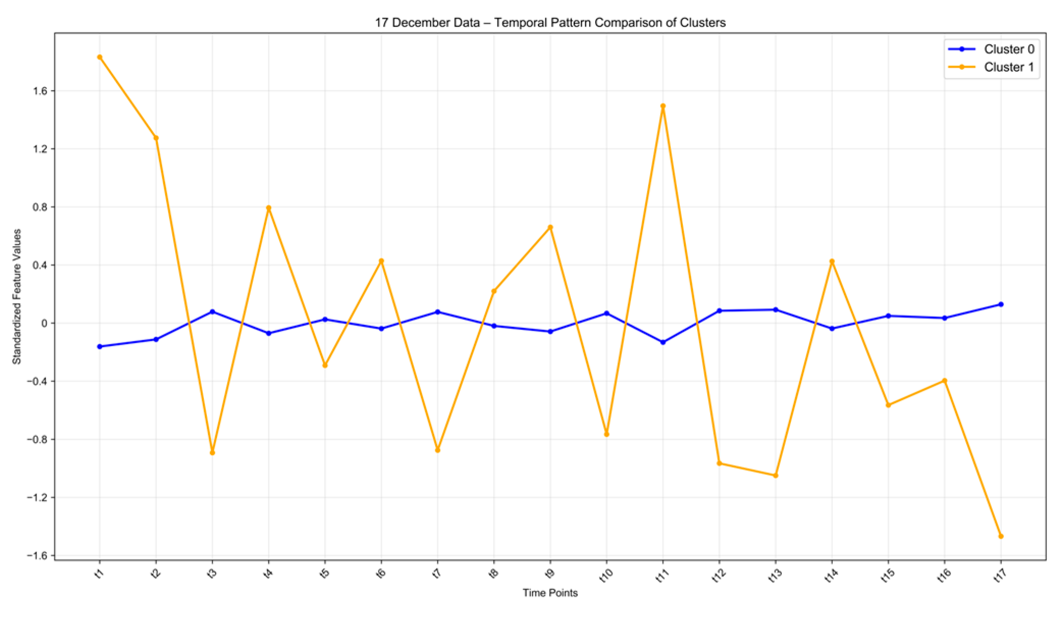
Temporal Pattern Comparison of Clusters on the Peak Season Weekday.
Figure 18.
Temporal Pattern Comparison of Clusters on the Peak Season Weekday.
Figure 19.
Spatial Clustering Analysis Results of Population Activity on an Off-Season Weekend (22 March). The green lines depict the temporal variation in standardized aggregation values across all regions. (a) Cluster 0. (b) Cluster 1.
Figure 19.
Spatial Clustering Analysis Results of Population Activity on an Off-Season Weekend (22 March). The green lines depict the temporal variation in standardized aggregation values across all regions. (a) Cluster 0. (b) Cluster 1.
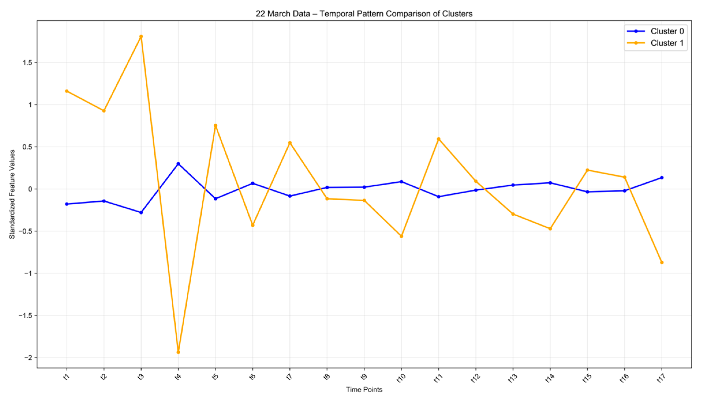
Figure 20.
Temporal Pattern Comparison of Clusters on Off-Season Weekend (22 March).
Figure 20.
Temporal Pattern Comparison of Clusters on Off-Season Weekend (22 March).
Table 1.
Data Sources and Preprocessing Description.
Table 1.
Data Sources and Preprocessing Description.
| Specific Data Name | Data Content Description | Data Format/Source | Brief Description of Processing |
|---|
| Basic Geographic Data | Administrative Boundary Data | Administrative boundaries at various levels | GADM Global Administrative Areas Database | Used to define the study area, serving as the base for spatial analysis |
| Road Traffic Data | Road type, location, length, name, etc. | openstreetmap | Used to calculate road network density, build network datasets, and perform sDNA analysis |
| Building Footprint Data | Building footprint, height | Crawled from Tianditu Platform | Used for calculating building density and floor area ratio within the fishnet grid. |
| POI | Central City POI Data | Address, administrative district, type | Crawled via Baidu Maps API | Classified by type, used to calculate facility density, function mix index, and other metrics |
| Bus and metro Stop Data | Station names, latitude, and longitude | Crawled from Baidu Maps | Used for public transport accessibility analysis |
| Socioeconomic Data | Residential Property Price Data | Average property price within unit grid | Numerical | Used to analyze the spatial differentiation of housing prices and its influencing factors |
Table 2.
Explanation Data and Sources.
Table 2.
Explanation Data and Sources.
| Built Environment | Data Sources | Indicator | Explanation |
|---|
| Construction Intensity | Building Footprint Data | Building Density | Total Base Area/Site Area |
| | FAR | Total Floor Area/Site Area |
| Land Use | Infrastructure POI Data | Land Use Mix | Shannon Entropy |
| Kernel Density of Infrastructure | Kernel Density |
| POI Density | Number of Facilities/Grid Cell Area |
| Transportation Accessibility | Road network data | Road Network Density | Road Length within the Grid Cell/Grid Cell Area |
| Road Accessibility | Closeness Metric Calculated based on the sDNA Model |
| Road Betweenness | Betweenness Metric Calculated based on the sDNA Model |
| Public transport POI | Distance to the Nearest Public Transport Stop | Distance from the Grid Cell Centroid to the Nearest Metro/Bus Station |
| Socioeconomic Factors | Residential Unit Price | house price | Average housing price within the grid cell |
Table 3.
General G statistics of population flow (Peak vs. Off-season).
Table 3.
General G statistics of population flow (Peak vs. Off-season).
| Statistical Metric | Observed General G: | Expected General G: | Variance: | z-Score: | p-Value: |
|---|
| PEAK | 0.000006 | 0.000002 | 0.000000 | 74.108732 | 0.000000 |
| LOW | 0.000005 | 0.000002 | 0.000000 | 72.795889 | 0.000000 |
Table 4.
Comparison of Model Performance between OLS and GWR during the Peak Season.
Table 4.
Comparison of Model Performance between OLS and GWR during the Peak Season.
| | R2 | R2 Adjusted | AICc |
|---|
| OLS | 0.67942792448 | 0.67892506632 | 127,265.26724200 |
| GWR | 0.736056 | 0.723182 | 126,465.488768 |
Table 5.
Spatial Autocorrelation Analysis Results of Residuals from the OLS and GWR Models during the Peak Season.
Table 5.
Spatial Autocorrelation Analysis Results of Residuals from the OLS and GWR Models during the Peak Season.
| Model | Analysis Object | Moran’s I | z-Score | p-Value | Spatial Pattern Judgment |
|---|
| OLS | Residuals | 0.168 | 18.97 | <0.001 | Highly Significant Clustering (Non-Random) |
| GWR | Residuals | 0.088 | 9.90 | <0.001 | Significant Clustering (But Weakened) |
Table 6.
Comparison of Model Performance between OLS and GWR during the Off-Season.
Table 6.
Comparison of Model Performance between OLS and GWR during the Off-Season.
| | R2 | R2 Adjusted | AICc |
|---|
| OLS | 0.68381014151 | 0.68326447341 | 128,460.32926700000 |
| GWR | 0.740531 | 0.726046 | 127,708.172418 |
Table 7.
Spatial Autocorrelation Analysis Results of Residuals from the Off-season OLS and GWR Models.
Table 7.
Spatial Autocorrelation Analysis Results of Residuals from the Off-season OLS and GWR Models.
| Model | Analysis Object | Moran’s I | z-Score | p-Value | Spatial Pattern Judgment |
|---|
| OLS | Residuals | 0.156 | 17.56 | <0.001 | Highly Significant Clustering (Non-Random) |
| GWR | Residuals | 0.075 | 8.43 | <0.001 | Significant Clustering (But Weakened) |
Table 8.
Factor detector results for population gathering–dispersal intensity in the peak season.
Table 8.
Factor detector results for population gathering–dispersal intensity in the peak season.
| | A | B | C | D | E | F | G | H | I |
|---|
| q statistic | 0.293 | 0.293 | 0.439 | 0.439 | 0.531 | 0.491 | 0.4821 | 0.360 | 0.191 |
| p value | 0 | 0 | 0 | 0 | 0 | 0 | 0 | 0 | 0 |
Table 9.
Interaction detector results for factors influencing population gathering–dispersal intensity in the peak season.
Table 9.
Interaction detector results for factors influencing population gathering–dispersal intensity in the peak season.
| | A | B | C | D | E | F | G | H | I |
|---|
| A1 | 0.293 | | | | | | | | |
| B1 | 0.405 | 0.293 | | | | | | | |
| C1 | 0.531 | 0.500 | 0.439 | | | | | | |
| D1 | 0.474 | 0.452 | 0.509 | 0.385 | | | | | |
| E1 | 0.599 | 0.581 | 0.588 | 0.602 | 0.531 | | | | |
| F1 | 0.538 | 0.523 | 0.544 | 0.526 | 0.622 | 0.491 | | | |
| G1 | 0.538 | 0.521 | 0.569 | 0.561 | 0.595 | 0.610 | 0.482 | | |
| H1 | 0.450 | 0.432 | 0.476 | 0.473 | 0.567 | 0.522 | 0.526 | 0.360 | |
| I1 | 0.330 | 0.356 | 0.490 | 0.442 | 0.561 | 0.512 | 0.521 | 0.407 | 0.191 |
Table 10.
Factor detector results for population gathering–dispersal intensity in the off-season.
Table 10.
Factor detector results for population gathering–dispersal intensity in the off-season.
| | a | b | c | d | e | f | g | h | i | j | k |
|---|
| q statistic | 0.200 | 0.299 | 0.381 | 0.544 | 0.510 | 0.121 | 0.464 | 0.375 | 0.513 | 0.304 | 0.456 |
| p value | 0 | 0 | 0 | 0 | 0 | 0 | 0 | 0 | 0 | 0 | 0 |
Table 11.
Table Interaction detector results for factors in the off-season.
Table 11.
Table Interaction detector results for factors in the off-season.
| | a | b | c | d | e | f | g | h | i | j | k |
|---|
| a1 | 0.200 | | | | | | | | | | |
| b1 | 0.365 | 0.299 | | | | | | | | | |
| c1 | 0.441 | 0.453 | 0.381 | | | | | | | | |
| d1 | 0.575 | 0.591 | 0.596 | 0.544 | | | | | | | |
| e1 | 0.532 | 0.542 | 0.538 | 0.637 | 0.510 | | | | | | |
| f1 | 0.274 | 0.352 | 0.419 | 0.557 | 0.539 | 0.121 | | | | | |
| g1 | 0.506 | 0.503 | 0.541 | 0.594 | 0.593 | 0.479 | 0.464 | | | | |
| h1 | 0.426 | 0.447 | 0.487 | 0.581 | 0.541 | 0.400 | 0.513 | 0.375 | | | |
| i1 | 0.544 | 0.532 | 0.559 | 0.630 | 0.596 | 0.525 | 0.561 | 0.536 | 0.513 | | |
| j1 | 0.344 | 0.417 | 0.480 | 0.606 | 0.558 | 0.338 | 0.525 | 0.465 | 0.549 | 0.304 | |
| k1 | 0.511 | 0.519 | 0.515 | 0.605 | 0.564 | 0.490 | 0.564 | 0.492 | 0.578 | 0.552 | 0.456 |
Table 12.
Factor detector results for Influencing Population Gathering–Dispersal Intensity in the Peak Season Weekday.
Table 12.
Factor detector results for Influencing Population Gathering–Dispersal Intensity in the Peak Season Weekday.
| | a1 | b1 | c1 | d1 | e1 | f1 | g1 | h1 | i1 | j1 |
|---|
| q statistic | 0.179 | 0.300 | 0.340 | 0.001 | 0.459 | 0.124 | 0.429 | 0.364 | 0.288 | 0.417 |
| p value | 0.000 | 0.000 | 0.000 | 0.1542 | 0.000 | 0.000 | 0.000 | 0.000 | 0.000 | 0.000 |
Table 13.
Interaction Detector Results for Factors Influencing Population Gathering–Dispersal Intensity in the Peak Season Weekday.
Table 13.
Interaction Detector Results for Factors Influencing Population Gathering–Dispersal Intensity in the Peak Season Weekday.
| | a1 | b1 | c1 | d1 | e1 | f1 | g1 | h1 | i1 | j1 |
|---|
| a1 | 0.179 | 0 | 0 | 0 | 0 | 0 | 0 | 0 | 0 | 0 |
| b1 | 0.35 | 0.3 | 0 | 0 | 0 | 0 | 0 | 0 | 0 | 0 |
| c1 | 0.395 | 0.424 | 0.34 | 0 | 0 | 0 | 0 | 0 | 0 | 0 |
| d1 | 0.182 | 0.303 | 0.344 | 0.001 | 0 | 0 | 0 | 0 | 0 | 0 |
| e1 | 0.481 | 0.496 | 0.485 | 0.465 | 0.459 | 0 | 0 | 0 | 0 | 0 |
| f1 | 0.256 | 0.35 | 0.379 | 0.132 | 0.487 | 0.124 | 0 | 0 | 0 | 0 |
| g1 | 0.463 | 0.473 | 0.494 | 0.433 | 0.531 | 0.446 | 0.429 | 0 | 0 | 0 |
| h1 | 0.404 | 0.435 | 0.448 | 0.367 | 0.494 | 0.39 | 0.484 | 0.364 | 0 | 0 |
| i1 | 0.321 | 0.404 | 0.437 | 0.291 | 0.502 | 0.327 | 0.494 | 0.443 | 0.288 | 0 |
| j1 | 0.463 | 0.484 | 0.468 | 0.42 | 0.505 | 0.454 | 0.519 | 0.459 | 0.505 | 0.417 |
Table 14.
Factor detector results for Influencing Population Gathering–Dispersal Intensity on Off-Season Weekend (22 March).
Table 14.
Factor detector results for Influencing Population Gathering–Dispersal Intensity on Off-Season Weekend (22 March).
| | a1 | b1 | c1 | d1 | e1 | f1 | g1 | h1 | i1 | j1 |
|---|
| q statistic | 0.21 | 0.317 | 0.405 | 0.001 | 0.551 | 0.117 | 0.483 | 0.395 | 0.314 | 0.484 |
| p value | 0.000 | 0.000 | 0.000 | 0.542724 | 0.000 | 0.000 | 0.000 | 0.000 | 0.000 | 0.000 |
Table 15.
Interaction Detector Results for Factors Influencing Population Gathering–Dispersal Intensity on Off-Season Weekend (22 March).
Table 15.
Interaction Detector Results for Factors Influencing Population Gathering–Dispersal Intensity on Off-Season Weekend (22 March).
| | a1 | b1 | c1 | d1 | e1 | f1 | g1 | h1 | i1 | j1 |
|---|
| a1 | 0.21 | | | | | | | | | |
| b1 | 0.385 | 0.317 | 0 | | | | | | | |
| c1 | 0.468 | 0.48 | 0.405 | | | | | | | |
| d1 | 0.214 | 0.318 | 0.407 | 0.001 | | | | | | |
| e1 | 0.571 | 0.581 | 0.578 | 0.555 | 0.551 | | | | | |
| f1 | 0.277 | 0.361 | 0.433 | 0.121 | 0.569 | 0.117 | | | | |
| g1 | 0.524 | 0.525 | 0.567 | 0.487 | 0.622 | 0.496 | 0.483 | | | |
| h1 | 0.447 | 0.47 | 0.514 | 0.397 | 0.575 | 0.415 | 0.539 | 0.395 | | |
| i1 | 0.357 | 0.436 | 0.505 | 0.316 | 0.592 | 0.344 | 0.547 | 0.484 | 0.314 | |
| j1 | 0.54 | 0.548 | 0.547 | 0.486 | 0.6 | 0.511 | 0.591 | 0.52 | 0.578 | 0.484 |
