Comprehensive Value Evaluation of Rural Shared Energy Storage Based on Nash Negotiation

Abstract

As a vital support for sustainable energy power systems, shared energy storage has the potential to address challenges in energy storage within rural grids. Nevertheless, the comprehensive value of rural shared energy storage (RSES) exhibits scenario-dependent variations across operation models, and existing studies have neither revealed this sensitivity nor established a scientifically unified evaluation method. This study first identifies typical rural grid scenarios using the density-based spatial clustering of applications with noise (DBSCAN) algorithm and analyzes RSES operation models. Then, this paper creates a three-dimensional evaluation system of RSES based on environmental, social, and governance (ESG) concepts that support sustainable development goals. Furthermore, to reconcile conflicts between subjective and objective weights, this paper proposes a combination weighting method based on Nash negotiation, subsequently using an improved technique for order preference by similarity to an ideal solution (TOPSIS) for multi-attribute decision-making. Finally, this paper completes simulations and discussions by an improved IEEE 33 bus system. The decision-making trial and evaluation laboratory (DEMATEL) technique and sensitivity analysis validate the validity and feasibility of the method proposed from horizontal and vertical dimensions. Based on the results, preferred strategies of RSES currently are energy aggregation and service purchase, for which this study provides recommendations.

1. Introduction

1.1. Motivation

The energy storage system (ESS), as a key enabling technology for sustainable energy power systems, has commenced extensive development. Nevertheless, ESS in rural grids still encounters challenges, such as elevated costs, poor usage rates, and difficulties in coordinated regulation across diverse scenarios [1]. These issues not only hinder the promotion and application of ESS in rural power grids but also exacerbate energy poverty in rural areas, where residents struggle to access affordable and reliable modern energy services [2]. As an innovative business model based on tenets of the sharing economy, rural shared energy storage (RSES) integrates distributed renewable energy (DRE), centralized station ESS, distributed household ESS, and mobile energy storage units, creating a collaborative operation model that mitigates these challenges. The deployment of RSES is intrinsically aligned with the Sustainable Development Goals (SDGs), as it facilitates enhanced integration of clean energy sources and carbon emission reductions, thereby actively contributing to the global transition towards sustainable energy systems [3,4].

Currently, the operation of RSES has exhibited significant scenario dependency due to factors such as seasonal load fluctuations, growing penetration of DRE, and the relatively weak structure of rural grids, manifesting in scenarios such as periods of high photovoltaic (PV) output, irrigation-related peak demand or holidays. Recent studies have focused on optimization issues of RSES under a single operation model. In [5], the researchers validated the success of RSES in enhancing PV consumption rates via multi-scenario comparisons. In [6], the researchers analyzed the operation mechanisms of RSES in rural living and production scenarios.

However, existing studies have not systematically revealed the sensitivity and variability of the comprehensive value of RSES across different scenarios, nor have they developed a targeted operation model evaluation for typical scenarios. Therefore, it is imperative to conduct a comprehensive value evaluation on distinct operation models of RSES across typical scenarios, thus providing a decision-making basis for its regulation, policy design and market implementation.

1.2. Literature Review

The construction of an evaluation index system and a multi-attribute decision-making model are vital components of the comprehensive value evaluation [7].

Current studies on the index system emphasize the techno-economic aspect. F.J. proposes an economic benefit evaluation model for distributed energy storage systems that considers multiple custom power services [8]. D.M. et al. proposed an evaluation model covering battery efficiency and lifetime deterioration, stressing the importance of applying distinct indices across various scenarios [9]. Y.S. et al. evaluated the economic value of ESS across scenarios separately for the grid-side and microgrid [10,11]. S.C. et al. analyzed the effects of tariff rules and incentives on the ESS operation model, proposing an incentive method combining flexibility and reliability [12]. B.Z. et al. evaluated the worth of ESS in enhancing new energy utilization and boosting system flexibility and economy through parameter planning theory [13].

Additionally, certain studies have proposed indices of environmental value. Based on the systematic, full-life-cycle perspective emphasized in [14], Y.L. et al. quantified the carbon reduction potential linked to manufacturing, transportation and recycling [15]. Based on the core waste-to-resource principle, by focusing on optimizing the properties and unlocking the value of specific waste streams to displace virgin resources [16], S.D. et al. revealed the non-linear relationship between the energy storage scale and environmental benefits via a dual-indicator analysis of carbon reduction and the carbon payback period, offering a dynamic perspective for assessing the environmental value of storage systems [17]. X.Q. et al. incorporated concepts of environmental, social, and governance (ESG) into the evaluation model and analyzed the environmental value of ESS under time-of-use tariffs [18].

Regarding research on multi-attribute decision-making methods, X.X. et al. evaluated the technical and economic value of ESS by the analytic hierarchy process (AHP) [19]. W.S. et al. analyzed the comprehensive value of distribution-side ESS by the cumulative approximation method and the difference method [20]. S.X. uses the entropy weight method (EWM) to assign objective weights to different evaluation indices, enabling a comprehensive evaluation of each generator’s voltage support potential [21]. K.B. uses the fuzzy AHP to develop an evaluation model for investing in PV projects, incorporating the uncertainty and fuzziness of expert judgments [22].

To consider subjective preferences and objective attributes, Z.C. et al. developed a method for ESS in microgrids using linear weighting [23]. D.W. et al. conducted an evaluation model of the operational effect of grid-side ESS using game theory [24]. C.S. et al. optimized subjective and objective weights separately using the minimum relative entropy (MRE) theory and fuzzy cumulative prospect theory (FCPT), establishing a basis for the selection of ESS [25,26]. S.D. et al. employed equal weights and fuzzy hierarchical analysis to conduct a thorough life cycle value evaluation of shared energy storage (SES) [27,28].

An analysis of studies revealed that comprehensive value evaluation indices and methods for RSES have yet to establish a quantitative standard and evaluation framework that possesses widespread consensus. On the one hand, recent studies have not incorporated the unique benefits of RSES. On the other hand, there remains potential for enhancing the weight allocation mechanism of current methods, particularly in tackling multi-scenario issues, where the stability of weight distribution and the reliability of evaluations require improvement.

1.3. Contributions

This study proposes an evaluation method for assessing the comprehensive value of distinct operation models for RSES across typical scenarios. The main steps include (1) identifying typical rural grid scenarios using the density-based spatial clustering of applications with noise (DBSCAN) algorithm and analyzing operation models; (2) formulating a three-dimensional evaluation system covering low carbon, reliability and economic value, based on concepts of ESG that supports the SDGs; (3) establishing the combination weighting model based on Nash negotiation to resolve conflicts caused by subjective and objective weighting from AHP and EWM; and (4) applying an improved technique for order preference by similarity to an ideal solution (TOPSIS) to conduct longitudinal comparisons between evaluation schemes and objectives.

Based on the proposed method, this study utilizes the improved IEEE 33 bus system for the evaluation, identifying the current optimal RSES operation models. Meanwhile, this study conducts horizontal and vertical tests using the decision-making trial and evaluation laboratory (DEMATEL) technique and sensitivity analysis. The results confirm the validity and feasibility of the proposed method. Ultimately, this study concludes with practical recommendations.

2. Analysis of RSES Application Scenarios and Operation Models

2.1. Analysis of Typical Scenarios in Rural Grids Based on the DBSCAN Algorithm

In contrast with the intensive nature of urban power grids, rural grids exhibit high volatility, high loss rates, high vulnerability, low power supply reliability, low load density, and inadequate equipment usage. Accordingly, there is an urgent need for SES to mitigate swings, enhance efficiency, and bolster resilience.

The traits of rural grids exhibit significant scenario dependency, and the evolution patterns of rural grids are affected by various factors, including agricultural production cycles, climate variables, and user behavior [29]. The conventional scenario analysis method based on typical days mainly includes selection based on manual experience and simplification based on time slices [30]. The former refers to manually choosing seasonal extreme days or special event days. The latter refers to dividing the entire year into a limited number of “time slices,” where load data within each slice is averaged. However, this method overlooks the spatiotemporal coupling patterns and probabilistic distribution traits of load data, making it difficult to accurately reflect the complex variability in rural grids caused by the influencing factors mentioned above [31].

In contrast, the density-based spatial clustering of applications with noise (DBSCAN) algorithm, as an unsupervised machine learning method, can comprehensively capture the spatiotemporal coupling features and probabilistic distribution traits by automatically identifying arbitrarily shaped load clusters and effectively handling noise data [32]. This method enhances the objectivity and accuracy of scenario clustering while also providing a more reliable data foundation for the subsequent comprehensive value evaluation.

This paper directly adopts the DBSCAN algorithm from [30] for clustering due to space limitations. A set of daily load curves was constructed by using 8760 h of load data supported by the Chongqing power grid from a county-level power grid in China for 2024. To ensure the comparability of the load characteristics, the daily load curves were standardized based on the maximum daily load. The clustering results are shown in Figure 1.

Figure 1 exhibits the central position curves of load clusters. Scenario 1 shows evening peak traits with a maximum at 20:00. After 20:00, the load persists over 0.60. These signify sustained high demand during nighttime. Scenario 2 displays a double-peak trend, occurring at about 7:00 and 15:00, with reduced intensity in the morning compared with the evening. These show two periods of intensive energy consumption during each day. Scenario 3 shows a stable trend during daytime, with the load surpassing 0.80 from 9:00 to 16:00 and the peak-to-trough variation rate descending below 20%. Scenario 4 exhibits traits of nightly pulse clusters with brief spikes occurring from 21:00 to 04:00. Each pulse possesses a duration of around 1 to 2 h with peak values over 0.60. These indicate irregular and high-power demand during nighttime. Scenario 5 possesses a minimal probability. The daytime load consistently remains high, while the nighttime demand diminishes due to storage from DRE. Nonetheless, it still exceeds the usual level. These reveal that the devices operate constantly, aligned with persistent demands during extreme weather conditions.

This study defines five typical scenarios of rural grids using multi-scale clustering and external factors, in contrast to conventional scene classification methods based on electricity intensity. Scenario 1 represents rural living characterized by a singular evening peak that addresses concentrated energy consumption for dwelling illumination, appliances and so on. Scenario 2 depicts rural production with a dual-peak structure at dawn and dusk, which mirrors conventional agricultural operation cycles. Scenario 3 exhibits rural processing marked by a plateau-like high load during daytime hours, reflecting the constant-power, long-duration operation of processing devices. Scenario 4 reflects rural transportation, showing nighttime pulse group traits with sporadic high-power demand that align with the cyclical patterns of vehicles. Scenario 5 depicts an emergency sustaining high loads throughout the day. The traits reveal that the energy-consuming devices require a stable power source. The duration has a positive relationship with weather warning levels.

2.2. Analysis of SES Operation Models

SES employs public energy storage devices to serve users by aggregating dispersed resources. This study classifies SES operation models into six groups based on investment subjects, resource management strategies, and energy interaction scopes [33], as illustrated in

Table 1. Classic operation models of SES.

Operation Model	Investment Subject	Resource Management Strategy	Interaction Scope
Capacity allocation	All users	Pre-allocated capacity and self-managed	Among users
Energy aggregation	All users	Centralized scheduling and optimization	Among users
Capacity leasing	Third-party operator	Billing based on leased capacity	Operator’s control area
Service purchase	Third-party operator	Billing based on the charging and discharging service	Operator’s control area
Internal sharing	All users	Collaborative scheduling among user groups	Among users
External sharing	All users	Participation in grid scheduling	With external grids

.

The operation models offer distinct solutions for the implementation of SES across scenarios. Nevertheless, for decision makers, there is a lack of comprehensive value evaluation indices and scientific methods, alongside an absence of scenario suitability analyses for operation models. Consequently, there is an urgent need to formulate comprehensive value evaluation indices of RSES and evaluate its comprehensive value utilizing multi-attribute decision-making methods.

3. Formulation of Comprehensive Value Evaluation Indices of RSES Based on the ESG Concept

3.1. ESG Concept

The ESG concept is an assessment system that combines environmental, social, and governance aspects, and it is intrinsically linked to sustainable development [34]. Sustainable development aims to meet the needs of the present without compromising future generations’ ability to meet their own needs. ESG provides an actionable framework for achieving sustainable development goals by systematically evaluating project performance in environmental protection, social equity, and economic governance. The ESG concept is incorporated into comprehensive value evaluation due to its multidimensional value integration capability and alignment with the needs of rural grids, alongside its direct support of sustainable development goals, particularly those related to affordable and clean energy, climate action, and sustainable infrastructure [35].

Based on the ESG concept, this study formulates a three-dimensional evaluation system of “low carbon, reliability, and economy” to overcome the limits of single-dimensional evaluation and to advance the sustainable transformation of rural grids. In the environmental dimension, this study designs eight low-carbon indices to optimize energy structure and cut multiple pollutants. In the social dimension, this study designs five reliability indices, covering core parameters for the secure and stable operation of power grids. In the governance dimension, this paper designs nine economic indices, covering investment, return, and commercial viability, which integrate unique value to rural scenarios. This evaluation system provides a quantitative framework for evaluating the comprehensive value of RSES, considering the decarbonization transition, grid safety and stability, and commercial viability, as detailed below.

3.2. Low-Carbon Value

• Proportion of new energy power generation

$$A1=(E\mathrm{r}/Et)\times 100\%,$$

(1)

where $E\mathrm{r}$ represents actual outputs of new energy; $Et$ denotes the total power generation.

2.

Rate of new energy consumption

$$A2=(E\mathrm{u}/Et)\times 100\%,$$

(2)

where $E\mathrm{u}$ represents the actual consumption of new energy.

3.

Decreased coal consumption of thermal power units

$$A3=\left[rcoal\cdot Er\cdot \left(1-\alpha l\right)/\eta g\right]\cdot Pcoal,$$

(3)

where $rcoal$ denotes the coal consumption rate; $\eta g$ represents the grid transmission efficiency; $\alpha l$ indicates the loss rate of power plants; $Pcoal$ signifies the price of the standard coal.

4.

Decreased carbon dioxide emission

$$A4=44/12\cdot \left[\omega C\cdot mcoal\cdot \alpha ox\cdot \left(1-\eta C\right)\right]\cdot PC,$$

(4)

where $\omega C$ is the mass fraction of carbon; $mcoal$ is the quantity of coal combustion substituted; $\alpha ox$ is the carbon oxidation rate; $\eta C$ is the carbon capture rate.

5.

Decreased carbon monoxide emission

$$A5=\left[\beta CO\cdot \omega C\cdot mcoal\cdot \left(1-\eta comb\right)\right]\cdot PCO,$$

(5)

where $\beta CO$ is the conversion factor of carbon to CO; $PCO$ is the cost of CO management.

6.

Decreased sulfur dioxide emission

$$A6=32/16\cdot \left[\omega S\cdot mcoal\cdot \left(1-\eta FGD\right)\right]\cdot PSO2,$$

(6)

where $\eta FGD$ is the efficacy of desulfurization; $PSO2$ is the cost of $SO2$ treatment.

7.

Decreased nitrogen oxide emission

$$A7=46/14\cdot \left[\omega N\cdot mcoal\cdot f\cdot \left(1-\eta SCR\right)\right]\cdot PNOx,$$

(7)

where $f$ denotes the conversion ratio of nitrogen to $NOx$.

8.

Decreased particulate emission

$$A8=\left[Ac\cdot \omega ash\cdot mcoal\cdot \left(1-\eta ESP\right)\right]\cdot PPM,$$

(8)

where $Ac$ represents the ratio of respirable suspended particulate in ash.

3.3. Reliability Value

• Reliability of power supply

$$B1=(1-T\mathrm{o}/Tt)\times 100\%,$$

(9)

where $T\mathrm{o}$ is the aggregate user outage duration; $Tt$ is the overall duration of the period.

2.

Voltage eligibility rate

$$B2=\left[1-\left(T\mathrm{u}+T\mathrm{d}\right)/Tt\right]\times 100\%,$$

(10)

where $T\mathrm{u}$ and $T\mathrm{d}$ represent the cumulative durations during which the voltage surpasses the upper and lower thresholds, respectively; $Tt$ denotes the overall monitoring duration.

3.

Voltage deviation rate

$$B3=(\left|Ur-Un\right|/Un)\times 100\%,$$

(11)

where $Ur$ represents the actual voltage; $Un$ denotes the nominal voltage.

4.

Frequency deviation rate

$$B4=(\left|fr-fn\right|/fn)\times 100\%,$$

(12)

where $fr$ represents the actual frequency; $fn$ denotes the nominal frequency.

5.

Harmonic distortion rate

$$B5=(\sqrt{{\displaystyle \sum _{h-2}^{50}{U}_h^2}}/U1)\times 100\%,$$

(13)

where $U1$ denotes the fundamental voltage root mean square (RMS).

3.4. Economic Value

• Initial investment cost

$$C1={\displaystyle \sum _{i=1}^I\left[r{\left(1+r\right)}^D\right]/\left[{\left(1+r\right)}^D-1\right]\cdot \left[QiCi\left(ni+1\right)\right]},$$

(14)

where D is the planning timetable; r is the prime interest rate;$Qi$ is the storage capacity; $Ci$ is the unit capacity investment cost; $ni$ is the frequency of replacement [36].

2.

Land cost

$$C2=A\times Pl,$$

(15)

where A represents the footprint; $Pl$ denotes the unit cost of land lease or acquisition.

3.

Construction and installation cost

$$C3=\left(CB\times Q\right)+Cl,$$

(16)

where $CB$ is the unit capacity installation cost; $Cl$ is the cost of installation labor.

4.

Charging and discharging loss cost

$$C4={\displaystyle \sum \left(Ein-Eout\right)}\times Pg,$$

(17)

where $Pg$ signifies the power purchase price during charging.

5.

Equipment maintenance cost

$$C5=Q\times Pmt\times Nmt,$$

(18)

where $Pmt$ is the unit maintenance cost; $Nmt$ is maintenance visits.

6.

Shared leasing benefit

The shared leasing benefit is divided as follows [37]:

$$C6.1={\displaystyle \sum _{i=1}^I\left(Qa,i\times Pa\times Ta,i\right)},$$

(19)

$$C6.2={\displaystyle \sum _{d=1}^D\left(Eu,d\times Pu\times \eta r\right)},$$

(20)

$$C6.3={\displaystyle \sum _{i=1}^I\left(Qr,i\times Pr\times Tr,i\right)},$$

(21)

$$C6.4={\displaystyle \sum _{k=1}^K\left(Ek\times \mathsf{\Delta }Pk\times \gamma s\right)},$$

(22)

$$C6.5={\displaystyle \sum _{t=1}^T\left(Ei,t\times Pi\right)},$$

(23)

$$C6.6={\displaystyle \sum _{m=1}^M\left(Qe,m\times Pe\times Hu,m\right)},$$

(24)

where $Qa,i$ is the capacity assigned; $Pa$ is the rental unit price per capacity; $Ta,i$ is the rental duration; $Eu,d$ is the number of electricity utilized; $Qr,i$ is the assured capacity allocated; $Pr$ is the cost of capacity reservation; $Tr,i$ is the contract duration; $\mathsf{\Delta }Pk$ is the pricing differential for charging/discharging; $\gamma s$ is the ratio for sharing service charges.

7.

Peak and valley arbitrage benefit

$$C7={\displaystyle \sum Ed\times \left(Pp-Pv\right)}\times \eta r,$$

(25)

8.

Improved new energy consumption benefit

Taking the wind energy (WE) utilized by RSES over a year as an example:

$$Ew={\displaystyle \sum _{i=1}^{365}{\displaystyle \underset{tl1i}{\overset{tl2i}{\int }}fw\left(t\right)}} dt,$$

(26)

$$fw\left(t\right)=\left\{\begin{array}{c}0 , Pw\left(t\right)\le Pw \\ Pw\left(t\right)-Pw , Pw\le Pw\left(t\right)\le Pw+P\max \\ P\max , Pw\left(t\right)\ge Pw+P\max \end{array}\right.,$$

(27)

where $tl1i$ and $tl2i$ represent the start and stop moments; $fw\left(t\right)$ represents the WE stored at time t; $Pw$ indicates the WE utilized during the valley time capacity.

The benefit formula for RSES from the consumption of the WE is:

$$Cw=\lambda w\cdot Ew,$$

(28)

likewise, the benefit formula for RSES from the consumption of the PV is:

$$Cpv=\lambda pv\cdot Epv,$$

(29)

where $\lambda pv$ is the feed-in tariff of PV. The benefit formula of RSES from the utilization of new energy is the sum of $Cw$ and $Cpv$.

9.

Delayed grid upgrading benefit

$$C9=P\inf \cdot e\inf \cdot \left[1-\exp (-\mathsf{\Delta }Np)\right],$$

(30)

$$\mathsf{\Delta }N=\log \left(1+\lambda \right)/\log \left(1+\tau \right),$$

(31)

where $P\inf$ is the power of RSES to delay grid expansion; $e\inf$ is the cost of unit expanding power; $\mathsf{\Delta }N$ is the duration of deferring the grid upgrade. $\lambda$ is the peak shaving rate of RSES; $\tau$ is the annual growth rate of peak load.

4. Multi-Attribute Decision-Making Methods for the Comprehensive Value Evaluation of RSES

This study addresses the issue of weight bias stemming from subjective preferences in AHP and the reliance on objective information in EWM. It reconciles the conflict between subjective and objective weights by incorporating Nash negotiation theory. This combination weighting model is utilized to create an evaluation framework for the comprehensive value of RSES, employing an improved TOPSIS to support multi-attribute decision-making for the evaluation.

4.1. Subjective Weighting Based on AHP

• Establish the Hierarchy

The comprehensive value evaluation index system of RSES constructed in this paper is shown in Figure 2.

2.

Construct the judgment matrix

$$A=\left[\begin{array}{l}a11\hspace{1em}a12\hspace{1em}\dots \hspace{1em}a1n\\ a21\hspace{1em}a22\hspace{1em}\dots \hspace{1em}a2n\\ ⋮\hspace{1em}\hspace{1em}⋮\hspace{1em}\hspace{1em}\hspace{1em}\hspace{1em}⋮\\ an1\hspace{1em}an2\hspace{1em}\dots \hspace{1em}ann\end{array}\right],$$

(32)

where $aij$ represents the relative significance of the indices i and j, utilizing the nine-level scale.

3.

Conduct the consistency test

To avoid excessive subjective value mistakes, it is vital to assess the consistency of the judgment matrix. The largest eigenvalue of the judgment matrix can be calculated as follows:

$$\lambda \max =(1/n){\displaystyle \sum _{i=1}^n\left[\left(A\widehat{\omega }\right)i/\widehat{\omega }i\right]},$$

(33)

The consistency ratio coefficient is subsequently calculated based on $\lambda \max$:

$$CR=CI/RI,$$

(34)

where $RI=1.65$, $CI$ is the consistency indicator:

$$CI=\left(\lambda \max -n\right)/\left(n-1\right),$$

(35)

when $CR<0.1$, the judgment matrix fulfills the consistency criterion.

4.

Calculate subjective weights

$$\omega i={\left({\displaystyle \prod _{j=1}^{n}aij}\right)}^{1/n},$$

(36)

the vectors $\omega ={\left(\omega 1,\omega 2,\dots ,\omega n\right)}^T$ are standardized for calculating the subjective weights:

$$\widehat{\omega }i=\omega i/{\displaystyle \sum _{j=1}^n\omega j}$$

(37)

4.2. Objective Weighting Based on EWM

• Establish the index matrix

This paper sets the total number of evaluation schemes as m, the total number of evaluation indices as n, and the value of each index as $dij$. The objective matrix is as follows:

$$D=\left[\begin{array}{l}d11\hspace{1em}d12\hspace{1em}\dots \hspace{1em}d1n\\ d21\hspace{1em}d22\hspace{1em}\dots \hspace{1em}d2n\\ ⋮\hspace{1em}\hspace{1em}⋮\hspace{1em}\hspace{1em}\hspace{1em}\hspace{1em}⋮\\ dm1\hspace{1em}dm2\hspace{1em}\dots \hspace{1em}dmn\end{array}\right],$$

(38)

2.

Standardize the index matrix

$$gij=dij/\sqrt{{\displaystyle \sum _{i=1}^m{\left(dij\right)}^2}}$$

(39)

3.

Calculate characteristic weights

$$hij=\left(1+gij\right)/{\displaystyle \sum _{i=1}^m\left(1+gij\right)}$$

(40)

4.

Calculate entropy weights

$$kj=-{\displaystyle \sum _{i=1}^{m}hij\cdot \ln hij}/\ln n$$

(41)

5.

Calculate the coefficient of variation

$$pj=1-kj$$

(42)

6.

Calculate objective weights

$$qj=pj/{\displaystyle \sum _{j=1}^{n}pj}$$

(43)

4.3. Combination Weighting Based on Nash Negotiation

The traditional combination weighting method, based on linear weighting, achieves combined weighting by linearly averaging subjective and objective weights, which is straightforward but overlooks inherent conflicts and synergistic effects between weights, potentially leading to biased, unbalanced results. Moreover, the traditional combination weighting method based on game theory establishes a mathematical optimization model to minimize the deviations between the combined weight and each respective weight set, which does not account for their actual credibility differences. Minor weight changes in multi-scenario decision-making may lead to ranking reversals.

To address these issues, this study proposes the combination weighting method based on Nash negotiation. Nash negotiation is classified as a cooperative game aimed at optimizing the maximization of the incremental product of collective utilities. The method formulates the utility function and resolves the equilibrium allocation scheme on the Pareto optimal frontier, creating a solution that fulfills both individual rationality and collective optimality criteria, as demonstrated in Equation (44):

$$\left\{\begin{array}{l}\max {\displaystyle \prod _{i=1}^I\left(Ui-U_i^0\right)}\\ s.t.\hspace{1em}Ui\ge U_i^0\end{array}\right.,$$

(44)

where $Ui$ represents the benefit accrued by a participant following engagement in the negotiation and collaboration; $U_i^0$ signifies the point of impasse in the negotiation.

The method assumes participants possess symmetric bargaining power, whereas the credibility of subjective and objective weights is unequal in multi-attribute decision-making. This study introduces the asymmetric bargaining power parameter and develops a combination weighting model based on Nash negotiation, as illustrated in Equation (45):

$$\left\{\begin{array}{l}\max {\displaystyle \prod _{j=1}^m{\left(\frac{{\omega }_j^{*}}{{\omega }_j^S}\right)}^{\alpha }{\left(\frac{{\omega }_j^{*}}{{\omega }_j^O}\right)}^{1-\alpha }}\\ s.t.\hspace{1em}{\displaystyle \sum _{j=1}^m{\omega }_j^{*}=1 , {\omega }_j^{*}>0}\end{array}\right.,$$

(45)

where ${\omega }_j^{*}$, ${\omega }_j^S$ and ${\omega }_j^O$ represent the combined, subjective and objective weights of the index.

Therefore, the proposed combination weighting method based on Nash negotiation achieves a weight allocation on the Pareto optimal frontier that satisfies both individual rationality and collective optimality, effectively overcoming the stated limitations and ensuring fairness and stability in weight allocation via a cooperative negotiation mechanism.

4.4. Comprehensive Value Evaluation Based on an Improved TOPSIS

The classical TOPSIS ranks evaluation schemes based on their relative proximity to the positive ideal solution and the negative ideal solution, which are derived from the maximum and minimum values within the set of evaluation schemes. This approach is inherently a horizontal comparison between the evaluation schemes. Nevertheless, as for the comprehensive value evaluation of RSES, decision makers are more concerned with the gap between the current conditions of RSES and its target condition.

To address this, this study adopts an improved TOPSIS with two key improvements. On the one hand, the target solution, representing the external expectation or desired state, is integrated into the definition of the positive ideal solution as shown in Equations (48) and (49), which surpasses the data-driven positive ideal solution of the classical TOPSIS. On the other hand, the Manhattan distance is employed instead of the Euclidean distance to calculate the distance of each scheme from both positive and negative ideal solutions, as shown in Equations (50) and (51), which mitigates the squared amplification effect. These practical enhancements shift the evaluation from a relative comparison between evaluation schemes to an absolute assessment of the gap between the present and target states. The specific steps of the improved TOPSIS are as follows:

• Normalization of data processing

$$I_x^{h,S}=\left\{\begin{array}{l}\left(I_x^h-I_x^{Ideal-}\right)/\left(I_x^{Ideal+}-I_x^{Ideal-}\right) , \mathrm{Ix}\in \mathsf{\Omega }\mathrm{B}\\ \left(I_x^{Ideal+}-I_x^h\right)/\left(I_x^{Ideal+}-I_x^{Ideal-}\right) , \mathrm{Ix}\in \mathsf{\Omega }\mathrm{C}\\ 1-\left|I_x^h-I_x^f\right|/\max (\left|I_x^h-I_x^f\right|) , \mathrm{Ix}\in \mathsf{\Omega }\mathrm{F}\end{array}\right.,$$

(46)

where $\left|I_x^h-I_x^f\right|$ represents the absolute departure of all evaluation indices from the optimal value.

2.

Calculate the weighted normalized matrix

$$V_x^{h,S}=I_x^{h,S}\zeta x,$$

(47)

where $\zeta x$ represents the combined weight of the index that concerns the overall target level.

3.

Calculate the optimal positive and negative solutions

$$I_x^{Ideal+}=\max \left\{I_x^{tar},\underset{h=1,2,\dots ,H}{\max }{I}_x^h\right\},$$

(48)

$$I_x^{Ideal-}=\min \left\{\underset{h=1,2,\dots ,H}{\min }{I}_x^h\right\},$$

(49)

where $I_x^{tar}$ represents the target value; $I_x^h$ denotes the value of the benefit-based index. However, the optimal positive solution in the classical TOPSIS for the benefit-based index is defined as $I_x^{Ideal+}=\max I_x^h$ and the negative solution is defined as $I_x^{Ideal-}=\min I_x^h$.The adoption of the improved TOPSIS ensures the evaluation is not limited to comparing the relative strengths and weaknesses among the alternative schemes [38].

4.

Calculate the distance of each scheme from both positive and negative ideal solutions

To avoid the squared amplification effect of the Euclidean distance, this study employs the Manhattan distance formula as follows:

$$D_{Euc}^{h+}={\displaystyle \sum _{Ix\in \mathsf{\Omega }x}\left|V_x^{h,S}-V_x^{Ideal+,S}\right|},$$

(50)

$$D_{Euc}^{h-}={\displaystyle \sum _{Ix\in \mathsf{\Omega }x}\left|V_x^{h,S}-V_x^{Ideal-,S}\right|},$$

(51)

where $V_x^{Ideal+,S}$ and $V_x^{Ideal-,S}$ represent the weighted normalized positive and negative ideal solutions, respectively.

5.

Calculate the relative proximity of each evaluation scheme

$$C_{\mathrm{Re}}^{h+}=D_{Euc}^{h-}/\left(D_{Euc}^{h+}+D_{Euc}^{h-}\right),$$

(52)

in conclusion, this paper proposes a comprehensive value evaluation method for RSES, depicted in Figure 3.

Figure 3 illustrates the overall flowchart of the comprehensive value evaluation method of RSES. The proposed method begins with subjective weighting based on AHP, followed by objective weighting using EWM. Subsequently, a combination weighting model based on Nash negotiation theory is constructed to effectively balance the game conflicts between subjective and objective weights. Finally, an improved TOPSIS is applied for multi-attribute decision-making. This flowchart establishes a methodological basis for the subsequent simulation and discussion.

5. Computational Results and Discussion

5.1. Case Overview and Parameter Settings

To verify the method’s scientific validity and feasibility, this paper employs an improved IEEE 33 bus system as a case for simulation and analysis [39], as shown in Figure 4. The simulation was implemented on the MATLAB/Simulink platform (MATLAB_R2021a), a widely used tool for power system modeling and dynamic analysis, which supports the construction of the improved IEEE 33-bus system and multi-scenario operational simulations. The system’s rated bus voltage is 10 kV. A traditional power supply with a total capacity of 50 MW is connected at node 1, with a maximum load of 40+j20 MVA. Distributed PV power supplies with capacities of 8 MW, 6 MW, 7 MW, and 9 MW are connected at nodes 7, 16, 22, and 32, respectively. A distributed WE supply with a total capacity of 12 MW is connected at node 24. Lithium iron phosphate battery storage, with a total capacity of 25 MW, is configured at nodes 7, 16, 22, 24, and 32. The clustering scenario results from Section 2.1 are applied as input parameters.

Simultaneously, this study, grounded in the fundamental principle of “who invests, who benefits,” referenced the literature in [40,41,42,43,44,45] and employed a simplified model to analyze RSES across six operation models, all aimed at minimizing total energy costs. The capacity allocation operation model employs an equalization system, while the external sharing operation model allocates 20% of the energy storage capacity for market engagement. The electricity pricing policy of Chongqing province [46,47] and other key simulation parameters [48,49] of RSES are shown in

Table 2. Key simulation parameters.

Parameter Name	Value	Unit
Residential electricity consumption during peak hours	0.6283	CNY/kWh
Residential electricity consumption during flat hours	0.5283	CNY/kWh
Residential electricity consumption during low hours	0.3483	CNY/kWh
Industrial/commercial electricity consumption during peak hours	1.2960	CNY/kWh
Industrial/commercial electricity consumption during flat hours	0.8100	CNY/kWh
Industrial/commercial electricity consumption during low hours	0.3078	CNY/kWh
The unit capacity investment cost	1000	CNY/kWh
Economic service life	10	year
Discount rate	10	%
Charge–discharge efficiency	92	%
The range of the state of charge	20–90	%

.

5.2. Calculation of Weights

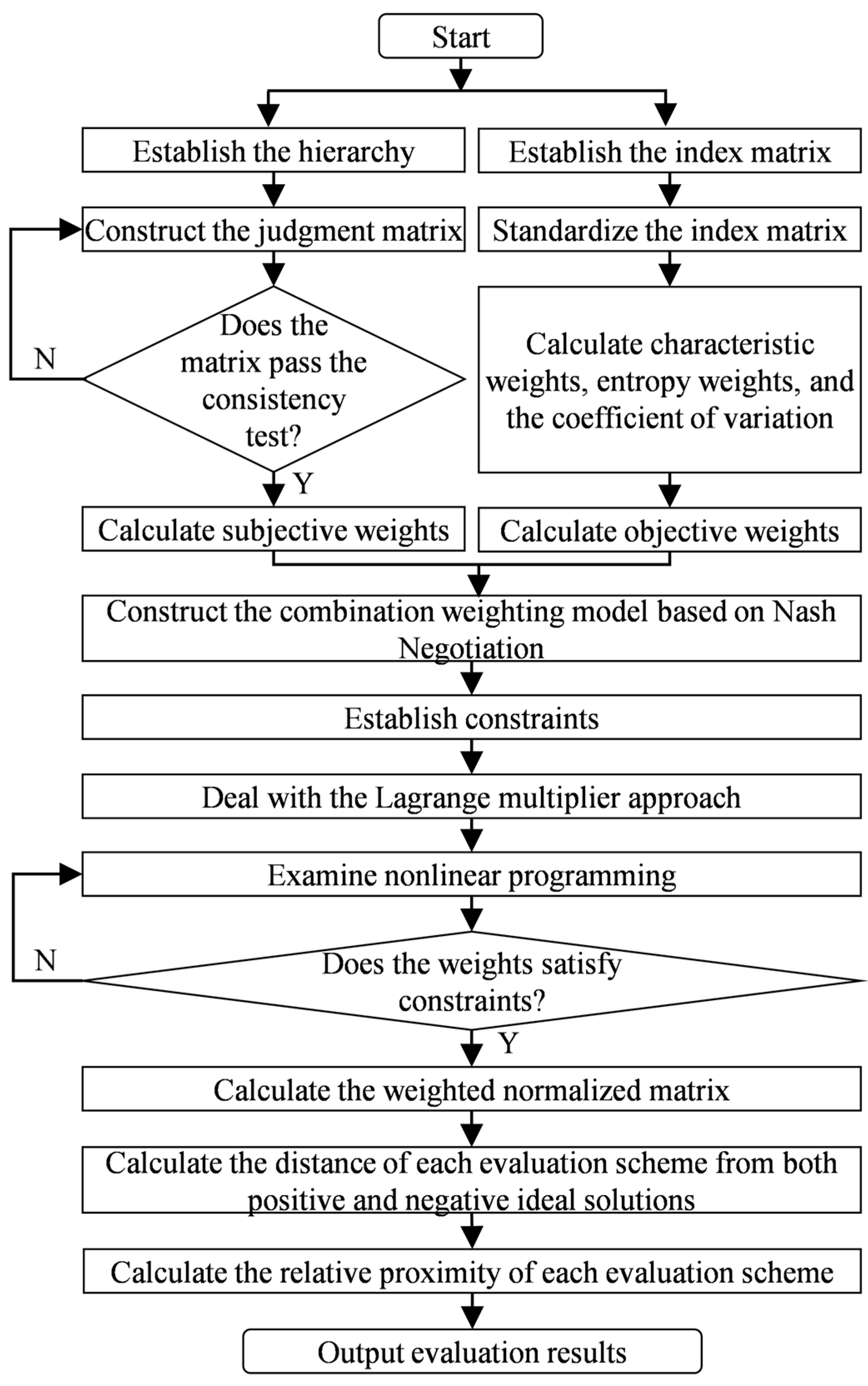
Seven experts were invited to assess the indices, which can be derived using Equations (33)–(35), as presented in

Table 3. Consistency ratio of expert evaluations across scenarios.

	Expert 1	Expert 2	Expert 3	Expert 4	Expert 5	Expert 6	Expert 7
Living	0.030	0.026	0.026	0.027	0.032	0.035	0.029
Production	0.030	0.027	0.031	0.031	0.036	0.030	0.024
Processing	0.023	0.034	0.025	0.028	0.027	0.036	0.022
Transportation	0.032	0.032	0.026	0.027	0.025	0.033	0.030
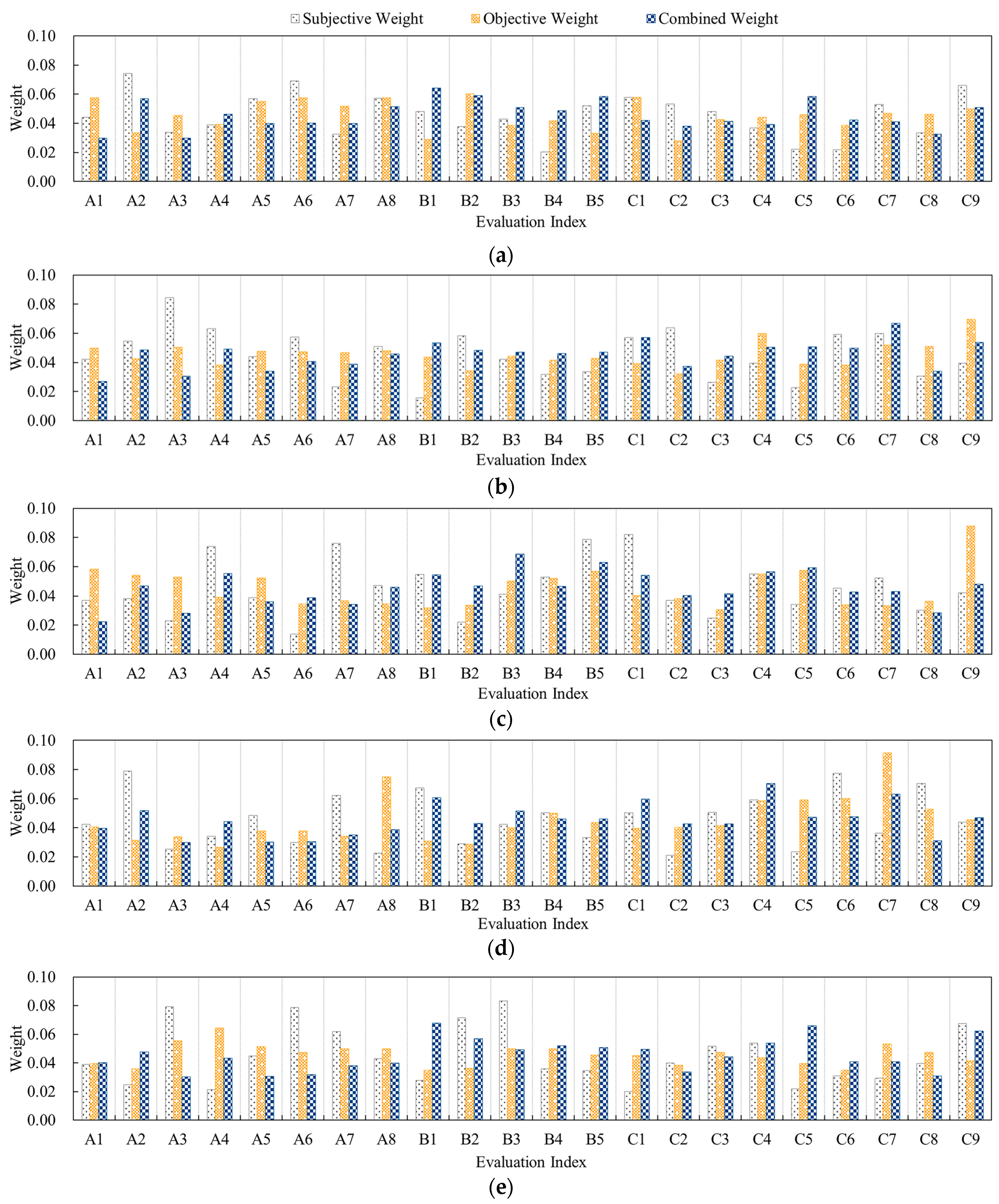
Emergency	0.031	0.026	0.032	0.019	0.036	0.033	0.034

. All satisfy the consistency requirements. The subjective, objective, and combined weights for the comprehensive value evaluation of RSES in each scenario can be derived from Equations (36)–(45), as demonstrated in Figure 5a–e.

As shown in Figure 5, the weight distribution is closely related to scenario traits. In the living scenario, the index with the highest subjective weight is A2, with a weight of 0.0744, reflecting the urgent demand for new energy consumption during evening peak loads. The index with the highest objective weight is B2, with a weight of 0.0604, demonstrating the emphasis on power supply quality in data-driven evaluations. The index with the highest combined weight is B1, with a weight of 0.0641, indicating that system reliability becomes the core concern after Nash negotiation coordination.

In the production scenario, the index with the highest subjective weight is A3, with a weight of 0.0844, highlighting experts’ preference for replacing traditional energy sources in agricultural production. The index with the highest objective weight is C9, with a weight of 0.0697, reflecting the objective value in deferring grid investments. The index with the highest combined weight is C7, with a weight of 0.0667, indicating that the traditional peak and valley arbitrage benefit remains the most dominant requirement after Nash negotiation coordination.

In the processing scenario, the index with the highest subjective weight is C1, with a weight of 0.0819, reflecting experts’ emphasis on cost control during long-term stable operation. The index with the highest objective weight is C9, with a weight of 0.0878, exceeding its weight in the production scenario, indicating the urgent need for rural grids to delay grid upgrading. The index with the highest combined weight is B3, with a weight of 0.0688, indicating that the requirement for voltage stability during continuous operation of processing equipment is the most prominent after Nash negotiation coordination.

In the transportation scenario, the index with the highest subjective weight is A2, with a weight of 0.0790, exceeding its weight in the living scenario, indicating the pulsed nighttime load traits of the transportation scenario impose more urgent demands for precise spatiotemporal alignment between new energy generation and load. The index with the highest objective weight is C7, with a weight of 0.0915, reflecting the objective significance of arbitrage opportunities. The index with the highest combined weight is C4, with a weight of 0.0705, indicating that loss costs become the primary consideration under frequent charge–discharge cycles.

In the emergency scenario, the index with the highest subjective weight is B3, with a weight of 0.0833, reflecting experts’ emphasis on power quality under extreme conditions. The index with the highest objective weight is A4, with a weight of 0.0644, highlighting the objective prominence of environmental value. The index with the highest combined weight is B1, with a weight of 0.0678, indicating that the power supply emerges as the core after Nash negotiation coordination.

These results validate the intrinsic consistency between weight allocation and scenario characteristics, providing a foundation for subsequent comprehensive evaluation.

Additionally, Figure 5 reveals that the results of the subjective, objective, and combined weights are not fully aligned due to the disparity between subjective preferences and data-driven objective responses resulting from distinct mechanisms of subjective and objective weighting systems. Employing the Nash negotiation model to optimize the allocation of subjective and objective utility can facilitate the alignment of interests and compensation between the two participants in the game.

5.3. Comprehensive Value Evaluation Results and Analysis

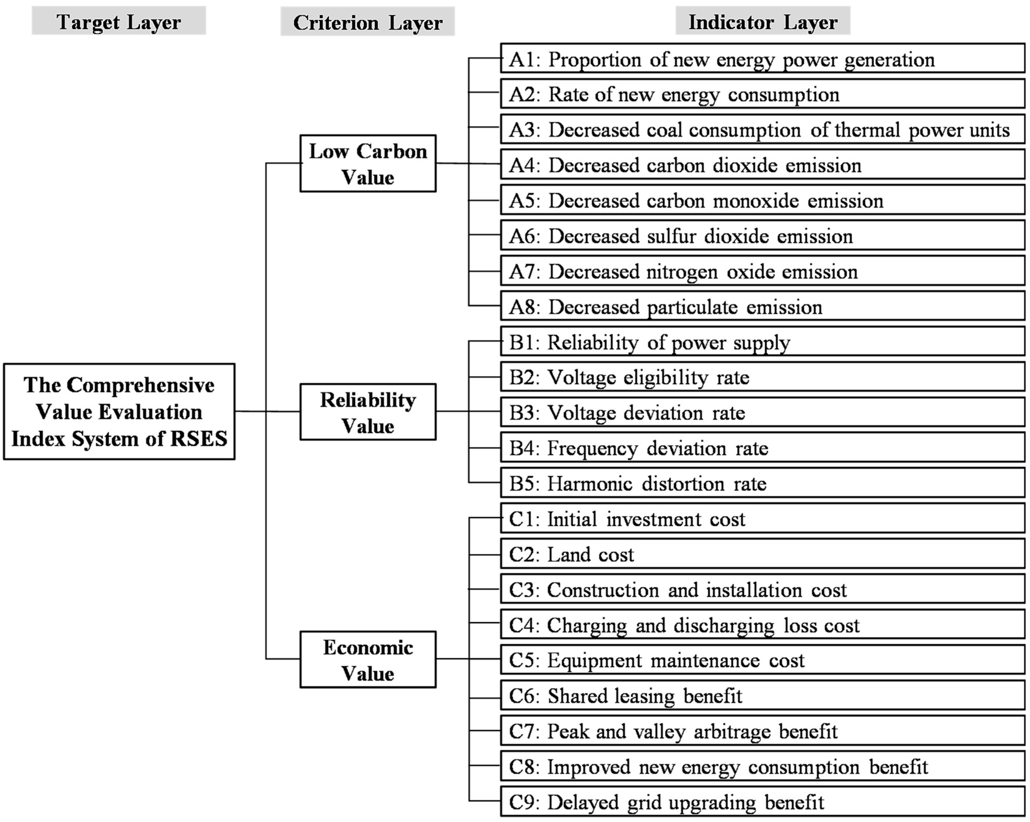
This study integrated the core tenets of China’s “carbon-neutral” objective for 2060 into the comprehensive value evaluation system of RSES. Under this target vision, the indices of low-carbon value, such as A1–A8, are directly benchmarked against the theoretical optimal values under a carbon neutrality pathway. For instance, the rate of new energy consumption approaches 100%, and emissions of carbon dioxide and other pollutants approach zero. The indices of reliability value, such as B1–B5, serve the security and stability requirements of a new power system with high penetration of renewable energy. For instance, the reliability of the power supply and the rate of voltage eligibility approach 100%, and the indices of power quality approach the optimal value. The indices of economic value, such as C1–C9, are defined by the anticipated technological advancement and market evolution under the objective. For instance, various costs approach the theoretical minimum under industry-leading technological constraints, while various benefits approach the theoretical maximum permitted by market mechanisms and system needs.

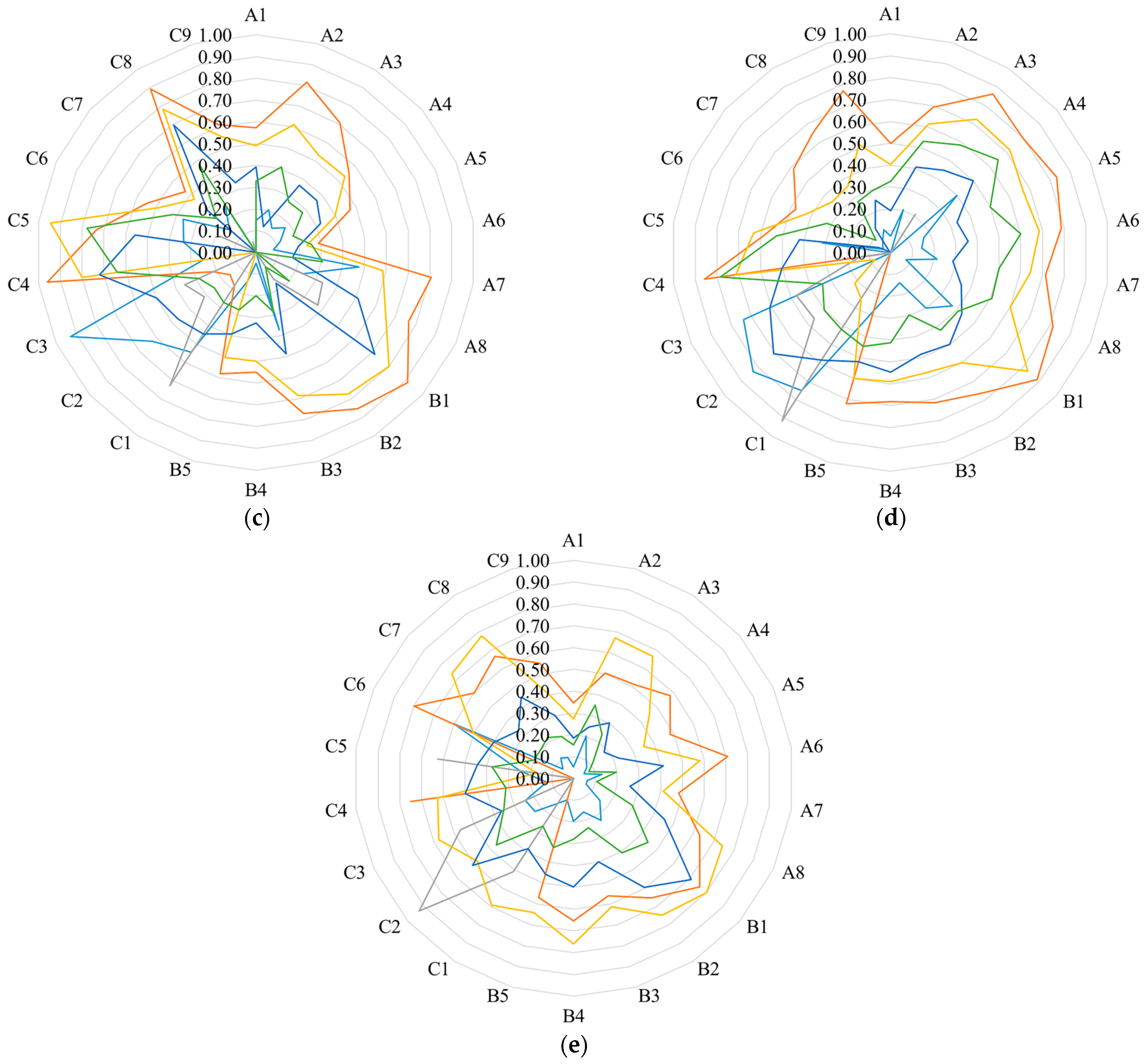
In the improved TOPSIS, the target values of the 22 indices across the three dimensions collectively constitute the target solution. The relative proximity of each operation model across several scenarios to the ideal solution can be calculated by applying Equations (46)–(52). The evaluation schemes 1 to 6 include capacity allocation, energy aggregation, capacity leasing, service purchase, internal sharing, and external sharing of the RSES operation model. The results of various scenarios are shown in

Table 4. The relative proximity of evaluation schemes in multi-scenario.

	Living		Production		Processing		Transportation		Emergency
	Relative Proximity	Rank	Relative Proximity	Rank	Relative Proximity	Rank	Relative Proximity	Rank	Relative Proximity	Rank
Capacity allocation	0.132	6	0.138	6	0.254	5	0.248	5	0.157	5
Energy aggregation	0.530	1	0.481	2	0.608	1	0.622	1	0.492	2
Capacity leasing	0.147	5	0.249	4	0.113	6	0.100	6	0.120	6
Service purchase	0.365	2	0.538	1	0.511	2	0.536	2	0.585	1
Internal sharing	0.340	3	0.374	3	0.388	3	0.392	4	0.395	3
External sharing	0.169	4	0.185	5	0.298	4	0.438	3	0.264	4

Footer: A Friedman test was conducted to assess the statistical significance of the rank differences in the six operation models across the five scenarios. The results indicate there is a statistically significant difference in the ranks between the models (${\chi }^2\left(5\right)=22.2,p<0.001$), confirming that the comprehensive value of RSES differs systematically across the operation models.

and Figure 6a–e.

This section analyzes the rural living scenario by taking Figure 6a as an example. In terms of low-carbon value, Schemes 2 and 4 perform better. Scheme 2 aggregates flexible resources most efficiently, with the relative proximity of 30.38% and 67.23% to new energy generation and consumption rates. Scheme 4 optimizes charging and discharging sequences, reducing annual coal usage to 37.50% of the target. While Scheme 1 performs the worst in new energy consumption due to capacity splitting, it reveals an inherent flaw in source–load matching. Regarding reliability, Scheme 2 excels in power quality indices, achieving a relative proximity of 94.74%. In contrast, Scenario 6 exhibits over twice the voltage/frequency deviation and harmonic distortion rate compared to Scheme 2. Economically, the optimization of source–grid–load–storage enhances peak shaving and valley filling in Scheme 2, covering nearly 20% of the initial investment and increasing the benefit of delayed grid upgrading to 42.11% of targets. However, Scheme 3 is hindered by accelerated charging and discharging cycle life decay, resulting in the relative proximity of charging and discharging loss cost of merely 22.73%.

A comparative analysis of the evaluation scheme rankings across the above scenarios reveals the following cross-scenario similarity patterns:

• Schemes 2 and 4 exhibit exceptional performance.

Scheme 2 incorporates flexible resources by SES, revealing success in living, processing, and transportation scenarios marked by load variability and sporadic access to high-power equipment, with the relative proximity values of 53.03%, 60.79%, and 62.23%. This aligns with the trend observed by C.J. et al. in their study on pricing strategies for user-side shared energy storage [50]. Moreover, Scheme 4 enhances charging and discharging strategies, demonstrating success in production and emergency scenarios that need rapid response and strict flexibility with the relative proximity of 53.79% and 58.50%.

• Schemes 5 and 6 exhibit moderate performance.

Scheme 5 exhibits superior economic performance by the peer-to-peer trading mechanism. However, the relative proximity of the peak and valley arbitrage is 26.30% due to the size and utilization efficiency. Simultaneously, Scheme 6 displays inferior reliability due to the impedance traits of rural grids, with the relative proximity to the voltage deviation rate index of only 22.98%.

• Schemes 1 and 3 exhibit poor performance.

Scheme 1 exhibits the relative proximity of 7.35% for the new energy consumption rate, due to inadequate spatial and temporal alignment of sources and loads. Meanwhile, Scheme 3 displays the relative proximity of 13.29% of the shared leasing benefit, owing to challenges in the formulation of pricing systems and economic forces. This aligns with the findings of H.Y. et al. that static lease contracts struggle to adapt to fluctuating energy supply and demand [51].

5.4. Testing

This study utilizes the DEMATEL technique for the horizontal validation and sensitivity analysis for the vertical validation to assess the success of the proposed method. Horizontal verification seeks to prove the method’s superiority by conducting cross-methodological assessments of the weight consistency and ranking stability. Vertical verification confirms the intrinsic resilience of the method by perturbing weight parameters.

• The DEMATEL technique for the horizontal validation

  (1)

  The DEMATEL technique

The DEMATEL technique is suitable for analyzing the interactions among factors within complex systems based on graph theory and matrix analysis [52]. By quantifying the intensity of both direct and indirect interactions among factors, each factor’s centrality and causality are calculated, revealing the system’s key factors and causal hierarchy. The calculation process of the DEMATEL technique is shown in the following steps [53]:

• (a)

  Construct and normalize the direct-relation matrix

$$X=Z/\underset{1\le i\le n}{\max }{\displaystyle \sum _{j=1}^n{z}_{ij}},$$

(53)

where $z_{ij}$ is the degree of direct influence of the index i on j. Z is the initial direct-relation matrix $Z={[z_{ij}]}_{n\times n}$, and it is obtained by using a 0–3 scale to rate the direct influences between indices.

• (b)

  Calculate the total-relation matrix

$$T={[t_{ij}]}_{n\times n}=X+X^2+X^3+\dots +X^{\infty }\approx X{(1-X)}^{-1},$$

(54)

• (c)

  Calculate the influence degree and affected degree

The sum of rows of the total-relation matrix is D, and the sum of columns of the total-relation matrix is R.

$$D={(d_i)}_{n\times 1}={\left[{\displaystyle \sum _{j=1}^n{t}_{ij}}\right]}_{n\times 1} , (1\le i\le n,1\le j\le n),$$

(55)

$$R={(r_i)}_{1\times n}={\left[{\displaystyle \sum _{j=1}^n{t}_{ij}}\right]}_{1\times n} , (1\le i\le n,1\le j\le n),$$

(56)

where $d_i$ represents the sum of the direct and indirect influences of index i on other indices and is called the influence degree of index i; $r_i$ represents the sum of the direct and indirect influences that index i receives from other indices and is called the affected degree of index i.

• (d)

  Calculate the center degree and cause degree of each index

$$g_i=d_i+r_i , (i=1,2,3,\dots n),$$

(57)

$$h_i=d_i-r_i , (i=1,2,3,\dots n),$$

(58)

where $g_i$ represents the center degree, indicating the position of the index i in the evaluation system and the size at which it works; $h_i$ represents the cause degree. If the cause degree is greater than zero, it indicates that the index i has a significant influence on other indices, and it is called the cause factor; conversely, it is called the result factor.

According to these steps, the central and causal degrees of each index can be calculated as presented in

Table 5. The central degree and causal degree of each evaluation index in the multi-scenario.

		A1	A2	A3	A4	A5	A6	A7	A8	B1	B2	B3
Living	$gi$	4.723	4.815	4.537	4.677	4.401	4.132	3.400	4.767	4.242	4.324	4.718
	$hi$	−1.249	0.055	−0.644	0.258	−0.711	0.711	0.198	−0.385	−0.356	−0.245	0.625
Production	$gi$	4.722	4.814	4.537	4.676	4.400	4.131	3.400	4.766	4.242	4.321	4.718
	$hi$	−1.249	0.055	−0.644	0.258	−0.711	0.711	0.198	−0.385	−0.355	−0.245	0.625
Processing	$gi$	4.714	4.808	4.531	4.672	4.394	4.114	3.394	4.759	4.237	4.317	4.714
	$hi$	−1.247	0.055	−0.644	0.257	−0.710	0.700	0.198	−0.384	−0.355	−0.244	0.624
Transportation	$gi$	4.723	4.816	4.537	4.676	4.401	4.131	3.400	4.766	4.243	4.322	4.717
	$hi$	−1.249	0.055	−0.644	0.258	−0.711	0.710	0.198	−0.385	−0.355	−0.245	0.625
Emergency	$gi$	4.707	4.806	4.523	4.662	4.388	4.112	3.389	4.755	4.232	4.308	4.704
	$hi$	−1.245	0.055	−0.643	0.257	−0.709	0.700	0.198	−0.383	−0.355	−0.244	0.623
		B4	B5	C1	C2	C3	C4	C5	C6	C7	C8	C9
Living	$gi$	6.260	4.844	4.602	3.580	5.731	4.144	4.184	3.768	4.518	4.245	3.832
	$hi$	−0.047	−0.257	−0.085	−0.167	−0.496	−0.468	0.753	0.214	1.781	−0.464	0.979
Production	$gi$	6.259	4.844	4.601	3.580	5.731	4.144	4.184	3.767	4.518	4.244	3.832
	$hi$	−0.047	−0.257	−0.085	−0.167	−0.497	−0.468	0.753	0.214	1.780	−0.464	0.979
Processing	$gi$	6.251	4.840	4.583	3.578	5.722	4.137	4.182	3.756	4.514	4.236	3.828
	$hi$	−0.047	−0.258	−0.075	−0.167	−0.495	−0.466	0.754	0.209	1.777	−0.463	0.978
Transportation	$gi$	6.259	4.844	4.601	3.580	5.730	4.144	4.185	3.767	4.518	4.245	3.832
	$hi$	−0.047	−0.257	−0.084	−0.167	−0.496	−0.468	0.753	0.214	1.781	−0.464	0.979
Emergency	$gi$	6.240	4.831	4.577	3.571	5.717	4.135	4.175	3.751	4.509	4.234	3.823
	$hi$	−0.046	−0.257	−0.076	−0.166	−0.494	−0.465	0.753	0.210	1.777	−0.463	0.976

.

• (2)

  Horizontal validation

This study validates the advantages of the proposed method using weight consistency verification and ranking stability verification.

• (a)

  Weight consistency verification

Based on the data in Table 5, this study calculates the Spearman rank correlation coefficient between the weights and the central degrees, which are calculated by the DEMATEL technique, to verify the weight consistency of the proposed method. This involved the weights derived from the method proposed in this study, as well as AHP, EWM, linear weighting [23], game theory [24], MRE theory [25], and FCPT [26]. The results are presented in

Table 6. Results of Spearman’s rank correlation test.

	Living	Production	Processing	Transportation	Emergency
The method proposed in this paper	0.706	0.666	0.722	0.674	0.710
AHP	0.307	0.227	0.265	0.306	0.306
EWM	0.349	0.306	0.290	0.245	0.316
Linear weighting	0.285	0.208	0.349	0.375	0.362
Game theory	0.485	0.407	0.549	0.491	0.471
MRE theory	0.490	0.455	0.451	0.477	0.433
FCPT	0.402	0.468	0.344	0.359	0.493

.

A greater absolute value of the Spearman rank correlation coefficient signals a stronger consistency in the weighting results. Table 6 reveals that the Spearman rank correlation coefficients of centralities and weights from this paper surpass those of other methods ($\rho >0.650,p<0.001$), with average enhancements of 31.97%, 32.08%, 34.73%, 29.85%, and 31.32% across the living, production, processing, transportation, and emergency scenarios, respectively. This suggests the weight assignment is more identical to the causal structural features.

• (b)

  Ranking stability verification

To validate the ranking stability of the proposed method, this study establishes a benchmark ranking derived from the weighted scores of standardized centralities. Subsequently, it computes the Kendall Tau-b correlation coefficient between these methods’ rankings and the benchmark ranking. The results are presented in

Table 7. Results of the Kendall Tau-b correlation test.

	Living	Production	Processing	Transportation	Emergency
The method proposed in this paper	1.000	0.867	1.000	0.867	1.000
AHP	0.200	0.067	0.067	0.200	0.200
EWM	0.333	0.200	0.067	0.067	0.200
Linear weighting	0.067	0.067	0.333	0.467	0.467
Game theory	0.867	0.467	0.867	0.867	0.867
MRE theory	0.867	0.600	0.600	0.867	0.600
FCPT	0.467	0.600	0.333	0.333	0.867

.

A higher absolute value of the Kendall Tau-b correlation coefficient indicates a more stable ranking. Table 7 reveals that the coefficients between the rankings from this study and datum rankings are superior to those of other methods ($\tau >0.850,p<0.001$), proving average improvements of 53.32%, 53.35%, 62.22%, 40.02%, and 46.65% across living, production, processing, transportation, and emergency scenarios, respectively. This indicates its rankings align most closely with the causal impact network.

2.

Sensitivity analysis for the vertical validation

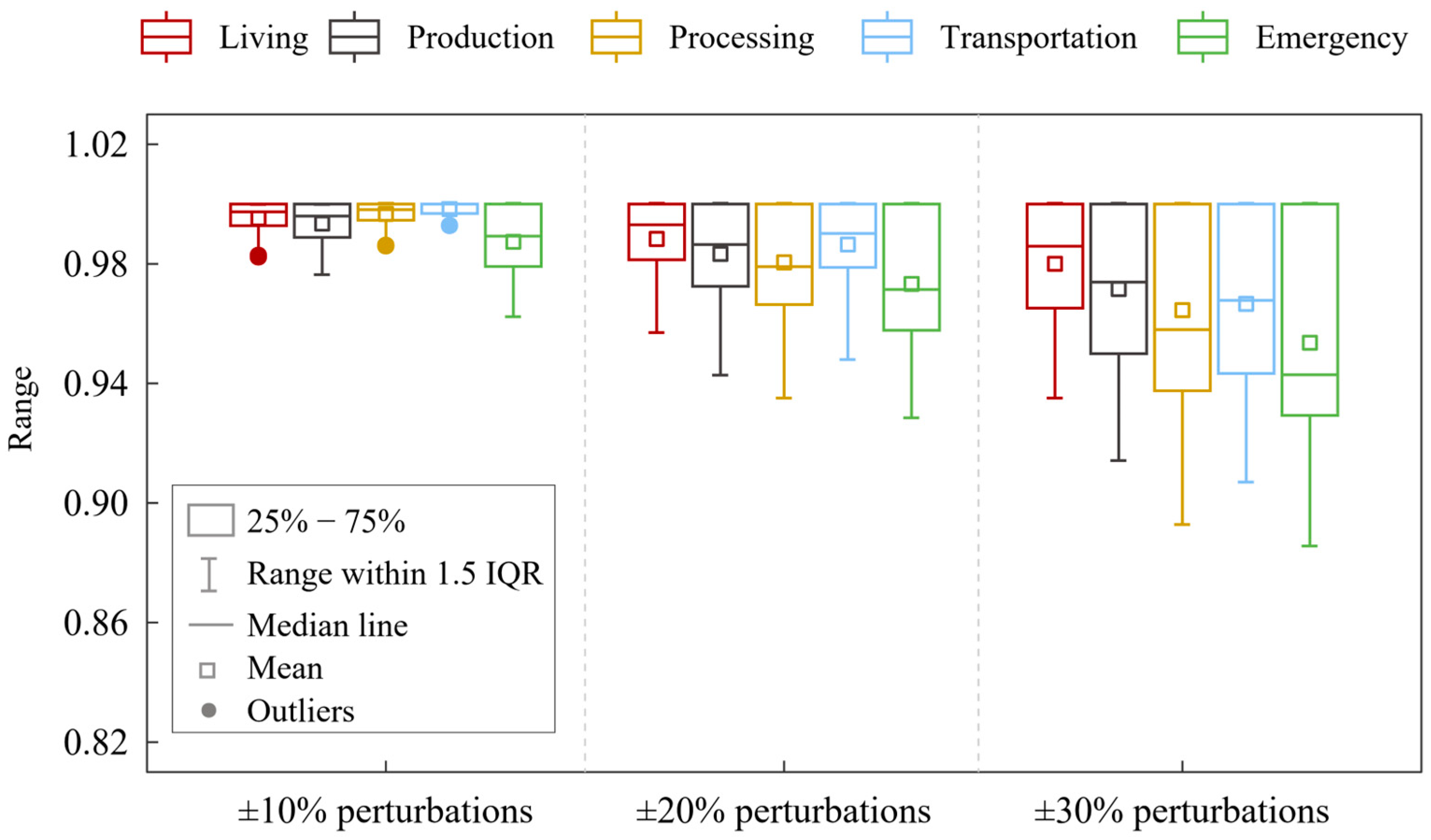
This section evaluates the resilience of decision results by applying ±10%, ±20%, or ±30% perturbations to the combined weights of each index and uses Spearman’s rank correlation coefficient to assess the ranking stability [54]. The results are shown in Figure 7.

Figure 7 illustrates that, in various scenarios, the median Spearman rank correlation coefficients of resultant rankings constantly exceed 0.94 relative to the original rankings when each weight is altered by ±10%, ±20%, or ±30%. This signifies that in over half of the perturbation scenarios, the ranking of evaluation schemes either remains constant or experiences only minor changes, demonstrating a high ranking stability of the proposed method.

Based on the sensitivity analysis involving three sets of perturbation experiments, the decision of the living scenario depicts the strongest stability in the experiments with ±20% and ±30% perturbations. This is because the load traits of this scenario are relatively stable, with a more evenly distributed combined weighting of its indices, avoiding excessive reliance on any single index. Moreover, the decision of the transportation scenario depicts the strongest stability in the experiments with ±10% perturbations. This is because the decisions are heavily influenced by fundamental economic indices. Accordingly, slight swings make it difficult to alter rankings. However, the emergency scenario shows the greatest sensitivity due to severe trade-offs between vital indices such as power supply reliability and initial investment cost. Various operation models have unique advantages across different indices, suggesting that changes in each weight may affect the relative ranks of evaluation schemes. Even so, these situations are rare, as the Spearman rank correlation coefficient remains high and no significant reversal in results occurs.

The preceding analysis illustrates that combination weights derived from Nash negotiation theory reconcile subjective experience with objective evidence effectively. The allocation allows the evaluation model to exhibit significant robustness when addressing uncertainties in parameter fluctuations.

In conclusion, the proposed method exhibits remarkable robustness and stability in rural scenarios. Its results provide solid data support and a decision-making basis for RSES operation models. However, this method is generally suitable for multi-attribute decision problems marked by conflicts in weight distribution, incorporating both subjective assessments and objective data. Appropriate alterations can be carried out by integrating this method with others, depending on the specific conditions of different fields.

5.5. Recommendations

• Technology

• Recommendation T1: Optimize the multi-stakeholder coordination and cross-scenario resource integration capabilities of the energy aggregation and service purchase operation models of RSES.

  (1)

  Data and results support

  The energy aggregation model ranks first in living, processing, and transportation scenarios, demonstrating consistent leadership in indices such as the reliability of power supply and the rate of new energy consumption. The service purchase model ranks first in production and emergency scenarios, demonstrating clear advantages in indices like the initial investment cost and the delayed grid upgrading benefit.

  (2)

  Specific measures

  For the energy aggregation model, develop a multi-agent collaborative scheduling algorithm to enhance the resource aggregation efficiency. For the service purchase model, develop a scene recognition algorithm for the charging–discharging strategy to strengthen flexibility and economic viability.

• Recommendation T2: Strengthen grid-connected power quality technologies for internal and external sharing operation models of RSES.

  (1)

  Data and results support

  Both internal and external sharing operation models generally exhibit poor reliability indices. For instance, in the living scenario, the relative proximity of the “voltage deviation rate” index of the external sharing drops to as low as 0.111, while the relative proximity of the “voltage eligibility rate” index of the internal sharing falls to 0.3125, representing critical shortcomings that constrain their comprehensive value.

  (2)

  Specific measures

  Establish stringent grid-connected power quality technical specifications and promote grid-forming energy storage technologies within both internal and external sharing operation models to provide robust voltage and frequency support for rural grids.

2.

Market

• Recommendation M1: Design priority access and green value monetization systems for the energy aggregation and service purchase operation models of RSES.

  (1)

  Data and results support

  Energy aggregation and service purchase represent the two operation models with the highest comprehensive value. For instance, energy aggregation demonstrates outstanding performance on indices such as the proportion of new energy power generation and the rate of new energy consumption. Service purchase makes significant contributions to indices such as decreased carbon dioxide emissions.

  (2)

  Specific measures

  Grant these models priority dispatch rights in electricity spot and ancillary service markets. Simultaneously, incentivize their active participation in carbon or green certificate markets to monetize their low-carbon value.

• Recommendation M2: Establish a performance-based compensation system to stimulate participation by internal and external sharing operation models.

  (1)

  Data and results support

  Although the internal and external sharing models rank moderately overall, they demonstrate potential in the revenue index, such as the equipment maintenance cost. However, their motivation for participating in rural grids remains insufficient.

  (2)

  Specific measures

  Quantify key parameters—such as regulation accuracy, response speed, and regulation stability—for ancillary services provided by the internal and external sharing operation models, using these indices as the core basis for settlement.

3.

Policy

• Recommendation P1: Implement guiding policies for the underperforming operation model of RSES.

  (1)

  Data and results support

  The capacity allocation and capacity leasing operational model consistently ranks poorly across most scenarios. The key issues lie in the low value of the rate of new energy consumption and the suboptimal returns from shared leasing.

  (2)

  Specific measures

  Develop scenario-specific access and restriction policies, and recommend integrating its operation with specialized services from other energy sectors.

• Recommendation P2: Introduce targeted incentive policies for the current preferred operation model of RSES.

  (1)

  Data and results support

  While the energy aggregation operation model offers high comprehensive value, its indices, such as the initial investment cost and the equipment maintenance cost, are relatively high, resulting in a higher initial investment threshold for operators and greater long-term operational and maintenance pressure.

  (2)

  Specific measures

  Provide investment tax rebates or operational subsidies for the energy aggregation and service purchase models based on effective aggregated capacity or actual service usage. This directly reduces initial investment burdens and accelerates the adoption of RSES’s current preferred operation model.

6. Conclusions

This paper proposes a quantitative evaluation method for the comprehensive value evaluation of operation models of RSES, based on typical scenarios identified using the DBSCAN technique. Existing studies have not systematically revealed the sensitivity of the comprehensive value of RSES across different scenarios, nor have they established a scientifically unified evaluation index system and decision-making method for typical scenarios. This paper addresses this issue according to the following three aspects: (1) an index system, including three dimensions—low carbon, reliability, and economy—and comprising 22 indices, was developed based on ESG concepts that support SDGs; (2) a combination weighting model was formulated using Nash negotiation theory, with subjective and objective weights derived from AHP and EWM being balanced; and (3) an improved TOPSIS was applied to facilitate multi-attribute decision-making across various scenarios. These provide new perspectives and methodological support for the comprehensive value evaluation of RSES, contributing to the sustainable transformation of rural grids.

Based on the method proposed, this paper took an improved IEEE 33 bus system as a case to evaluate and provided recommendations regarding technical, market, and policy aspects. The results are as follows:

• The method proposed passed horizontal and vertical tests, proving its scientific validity and feasibility. In the horizontal test with the DEMATEL technique, the method proposed outperformed all other compared methods regarding weight consistency and ranking stability. Specifically, the Spearman rank correlation test revealed a significant correlation between the weights from the proposed method and the centrality degree ($\rho >0.650,p<0.001$), demonstrating the most outstanding compatibility with the system’s causal structure features. The Kendall Tau-b correlation test proved that the ranking results from the proposed method were optimally aligned with the systematic causal influence network ($\tau >0.850,p<0.001$), exhibiting a correlation coefficient that significantly exceeds that of other methods. Additionally, in the vertical test with sensitivity analysis, the median Spearman rank correlation coefficients between rankings and original results consistently exceeded 0.94 when each weight was perturbed by ±10%, ±20%, or ±30%, showing the method’s great robustness.
• The operation models of energy aggregation and service purchase are the optimal strategies for RSES at present. The operation model of energy aggregation was most effective in rural living, processing, and transportation scenarios, with relative proximity values of 53.03%, 60.79%, and 62.23%. Simultaneously, the operation model of service purchase was optimal in rural production and emergency scenarios, with relative proximity values of 53.79% and 58.50%.

Future work will focus on elucidating the dynamic evolution of value evaluation across multiple scenarios and exploring model self-optimization methods utilizing operational data.