Revisiting Trend Stability Using Mann-Kendall and Wilcoxon Signed-Rank Tests Through Innovative Method Comparisons

Abstract

Understanding the persistence and stability of hydroclimatic trends is essential for climate adaptation and sustainable water resource management, particularly in Mediterranean regions characterized by irregular precipitation regimes. This study examines long-term rainfall variability (1974–2021) at six meteorological stations along the southern coasts of Türkiye using three complementary non-parametric techniques: the Mann-Kendall (MK) test, the Wilcoxon Signed-Rank Test (WT), and the Innovative Trend Analysis (ITA). The three tests were applied with their respective methodological extensions to enhance sensitivity and better capture trend stability. Results show that while most stations exhibit generally stable rainfall regimes, period- and location-specific variations with non-monotonic or oscillatory tendencies are present, revealing patterns that standard trend tests often fail to detect. The WT method was more responsive to short-term fluctuations, whereas ITA and its three-dimensional version (3D-ITA) provided valuable insights into trend persistence and stability. Overall, the findings highlight that trend stability assessment enables the distinction between transient climate variability and sustained hydroclimatic change, offering a stronger scientific basis for adaptive water management and regional sustainability planning under climate uncertainty.

1. Introduction

Identifying and understanding long-term changes in hydrological, hydroclimatological, and meteorological systems is vital for the assessment of variability in natural processes [1]. Recent changes in temperature, precipitation patterns, and the increasing number and severity of extreme events, including floods and droughts, illustrate the significance of investigating changes [2]. Recognizing that in some instances and in some locations, these changes impact the quantity, reliability, and spatial distribution of water resources, and pose a problem for planning, design, and sustainable management. In this context, investigating change in long-term records can provide critical information for risk assessment and decision-making pertaining to adaptation and resiliency in water infrastructure and ecological systems.

The importance of trend analysis is that it will detect directional change whether increasing, decreasing, or altering over time in time series data. Classical statistical methods have been employed for decades by researchers for identifying trends in hydrology and using non-parametric methods like the Mann-Kendall (MK) test [3,4], Sen’s slope estimator [5], and regression-based methods [6]. These methods are non-parametric, robust against outliers, and appropriate for hydrological datasets that can be skewed. A variety of hydrological analyses have applied these methods to identify trends in precipitation, streamflow, evaporation, and temperature across different geographical regions [7,8,9,10,11,12]. However, although those methods are effective in identifying monotonic (increasing or decreasing) trends, they are limited in identifying non-monotonic trends and in evaluating trends across sub-periods of long datasets.

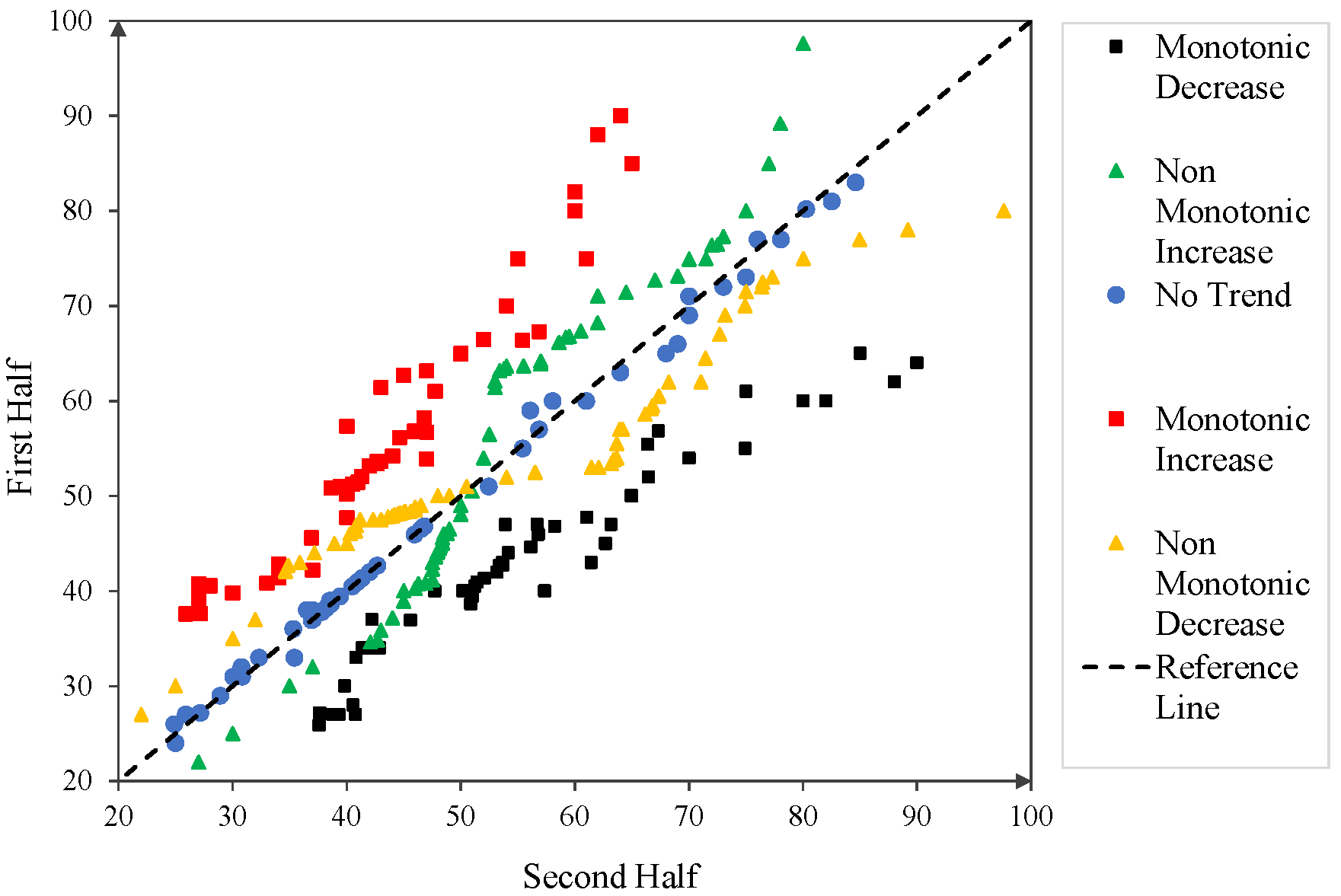
To address these limitations, Şen [13] introduced the Innovative Trend Analysis (ITA) method, which provides a flexible and visual framework for identifying both monotonic and non-monotonic changes. ITA divides a dataset into two equal halves, ranks the values, and plots them against each other along a 1:1 reference line. Depending on the distribution of data points relative to this line, ITA can classify trends into five categories: non-monotonic increase and decrease, monotonic increase and decrease, and no-trend cases. A major advantage of ITA is that it does not require assumptions of normality or independence of observations, unlike many classical statistical techniques. This makes ITA particularly attractive in hydrological applications, where time series often display skewness, seasonality, or serial correlation.

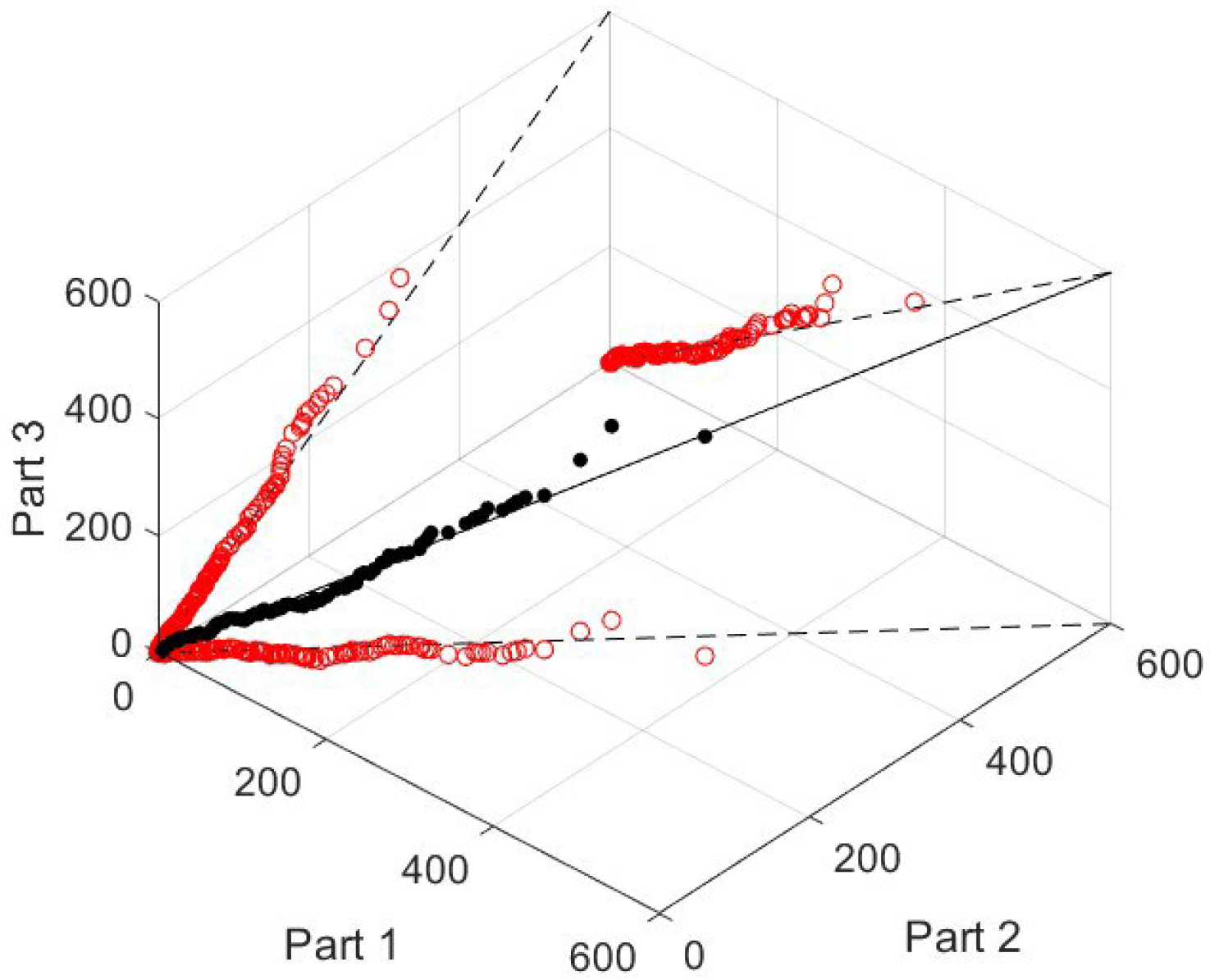
Several extensions to ITA have been proposed that build on its foundations, including double-ITA (D-ITA) and triple-ITA (T-ITA), which divide the time series into three and four equally spaced sub-periods, respectively, and allow for examining trend stability in different time segments [14,15,16]. A three-dimensional ITA (3D-ITA) offered by Güçlü [16] improves interpretability through projecting the three subseries into a three-dimensional coordinate system relative to the 1:1:1 line and makes it possible to simultaneously investigate both trend type and stability [17,18,19]. Alashan [20] provided refinements of ITA to increase flexibility, and Güçlü [14] extended ITA by coupling with frequency–intensity–duration curves for rainfall variability, as well as applying it to atmospheric pollutant records, characterized by air quality index classifications. These additions indicate that ITA is not applicable for revealing hidden or unstable trends, but it is versatile enough to be examining interrelated datasets using comparison-based frameworks.

Simultaneously, Tabari et al. [21] combined ITA with a quantile perturbation method, segmenting the time series into decadal intervals to analyze distributional differences in quantiles over successive time periods. These methodological contributions underscore the importance of analyzing hydroclimatic records on a smaller time scale, as opposed to reviewing the data as a whole. Analyzing smaller time units can provide more thorough insight into the changing persistence and variability of hydroclimatic trends. Collectively, these studies demonstrate that ITA-type methods produce a fuller and more holistic understanding of hydrological and meteorological records, including rainfall, streamflow, and temperature, by detecting hidden or uncertain elements of the record that would not be found through traditional approaches.

Alongside ITA-based methods, the Wilcoxon Signed-Rank Test (WT) has increasingly been used in hydroclimatic research. While it was developed specifically for paired-sample analysis [22], WT has been successfully adapted for trend detection, due to its non-parametric methodology and suitability for very small or non-normality datasets. When compared to ITA, the Wilcoxon matched-pairs approach assesses as a trend by splitting the time series up into two halves without disrupting their order. Saplıoğlu and Güçlü [23] have added to this method by examining degree of change visually by merging WT with scatter diagrams, thus improving both numerical and visual interpretation of hydrological records. Their study made a comparison of WT to Mann-Kendall (MK) test rules. They noted that WT produced comparable output to MK, and gave much greater ability to visualize subtle movement in trend behavior. Following earlier developments, Demirel et al. [17] introduced the Triple WT (T-WT), which incorporates the statistical robustness of WT within the three-dimensional design of the ITA. In this design, the dataset is divided into three equal-sized portions, WT is applied iteratively, thereby allowing a more granular investigation of persistence and stability with respect to trends. This perspective of the analysis, with attention on stability, addresses weaknesses that relying upon traditional approaches does not take into account. While traditional approaches, for example the MK, are important for detecting trends, the pairing of the ITA with Wilcoxon-based approaches enhances the trend detection of several different types and incorporates stability assessments, which are key for water resource management and adaptation for climate change [16,17,24].

In addition, several recent studies have increasingly employed non-parametric and novel statistical approaches to analyze hydroclimatic trends under a changing climate. Küçükerdem Öztürk et al. [25] illustrated that using the MK, WT, and graphical tests together might detect subtle and non-monotonic variations more effectively. Yüce et al. [26] and Akbaş et al. [27] noted that ITA and related tests can detect oscillating or transitioning behaviors in precipitation datasets to highlight rainfall behavior. Similarly, Topçu et al. [28] and Gezici et al. [29] confirmed that combining classical methods with new approaches improves the robustness of hydroclimatic variability assessments in Mediterranean-type regions. In spite of recent advancements, minimal attempts have been made to assess trend stability via multi-method evaluation, particularly within Türkiye’s southern coastal regions, a limitation that the current study resolves.

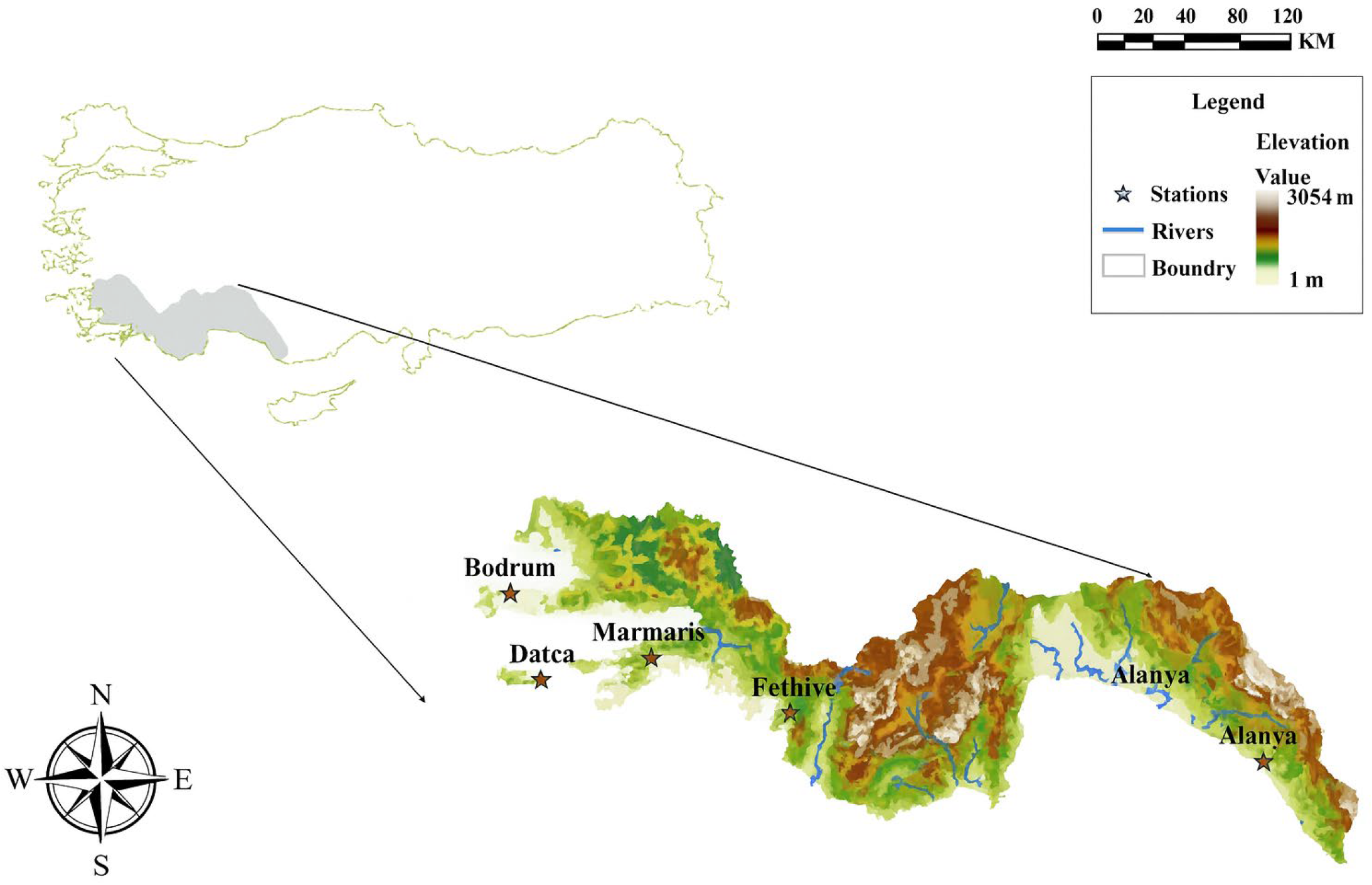
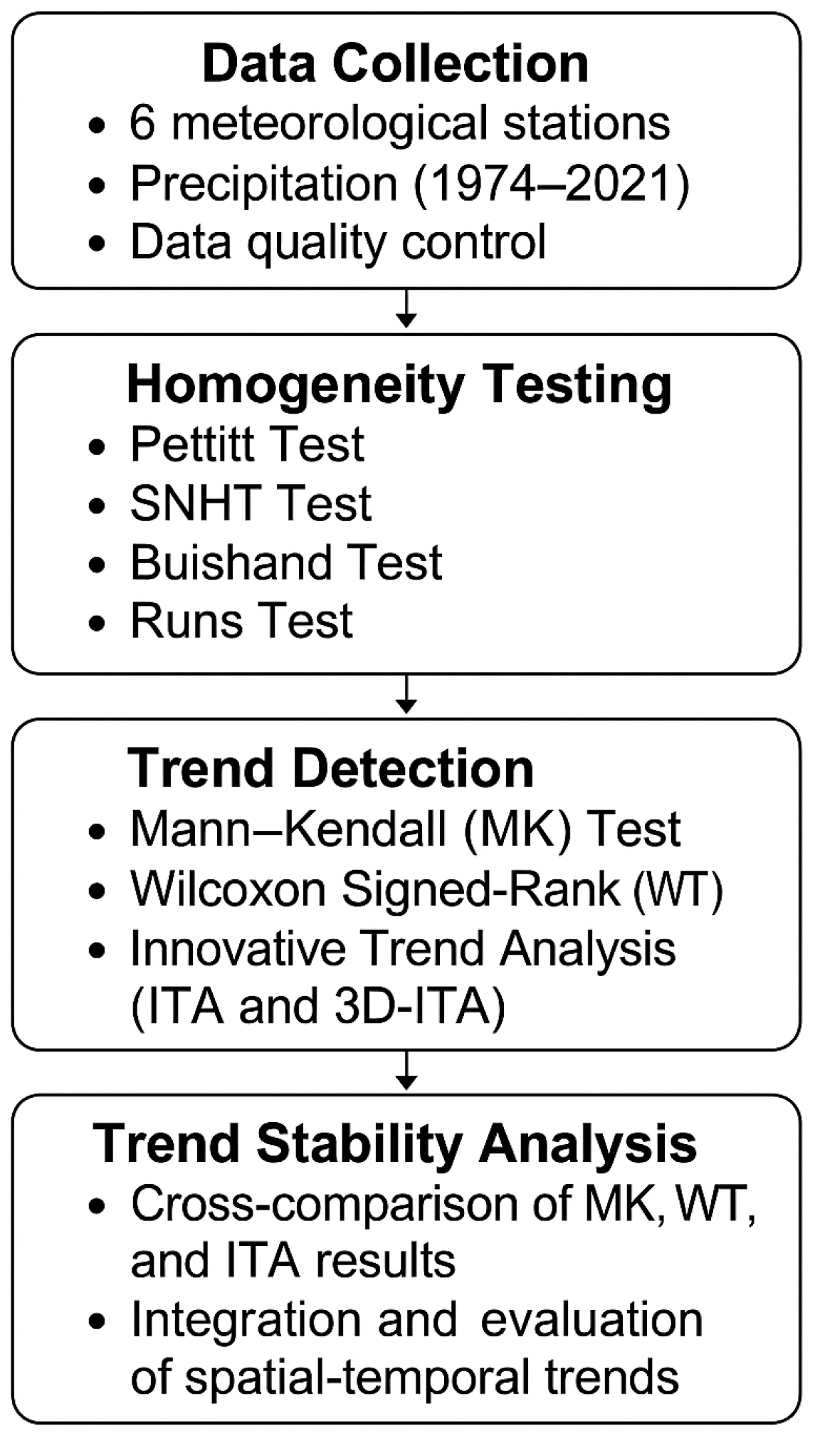
Briefly, the general objective of this study is therefore to identify and visualize the stability of trends in monthly rainfall records (1974–2021) at a number of stations along the south coast of Türkiye through extended versions of MK, Wilcoxon-based methods. In addition, the performance of these techniques will be compared with the standard and enhanced ITA versions for the purpose of determining their relative advantages and disadvantages. These new approaches will provide a more stable and stronger basis for assessing the persistence and intensity of hydroclimatic trends. In other words, the presented study introduces a comprehensive framework that integrates the MK, WT, and ITA methods to evaluate the stability and consistency of long-term precipitation trends. In contrast to earlier research which usually applied these approaches independently, the proposed method systematically compares the results from a range of methodologies to evaluate differences and methodological sensitivity to climatic and topographic contexts. This combined analysis improves the robustness of trend detection and offers new perspectives into the physical and statistical processes driving rainfall variability along the southern coast of Türkiye.

2. Materials and Methods

2.1. Study Area and Data

The study takes place at stations located along the southern coast of Turkey in Western Mediterranean and Antalya basins (Figure 1). These two adjoining basins have a total surface area of 39,909 km², located between the latitudes of 36°13′–38°28′ N and longitudes of 27°23′–32°22′ E [30]. The climate is primarily Mediterranean with warm, dry summers and mild winters with precipitation. The Central Anatolian continental climate factors into the climate of the inland regions of the Antalya Basin which brings cooler winters with snow expected. The summer mean temperature along the coast is about 28.2 °C with mean winter temperature falling to near 9.9 °C. Rainfall occurs annually in the amounts of 600 to 1000 mm—mostly in the winter months of frontal precipitation. Drought conditions occur as a part of the climate patterns of the Mediterranean climate and result from irregular precipitation. Topography also contributes to climate change elevations ranging from sea level up to 3060 m in the Western Mediterranean Basin and elevations to 3000 in the Antalya Basin.

In the presented study, monthly precipitation data measured by the Turkish State Meteorological Service (MGM) between 1974 and 2021 were analyzed from six meteorological observation stations. They were selected based on their data completeness, record length, and spatial representativeness. It is important to denote that the chosen stations account for coastal and near-inland locations in the study region and span lower elevations to mountainous foothills. This affords the opportunity to assess how topographic gradients from low-lying coastal plains and higher foothill locations could impact variations in precipitation and stability of trends across the region. Lastly, while all six stations have similar Mediterranean-type climate characteristics, they exist in different microclimatic settings in the study region. The geographical locations of the stations, along with key statistical properties of the observed data, are summarized in

Table 1. Meteorological station details.

Station	Station Name	Elevation (m)	Coordinates		Precipitation
			Latitude (N)	Longitude (E)	Average (mm)	Std. Deviation (mm)
17290	Bodrum	26	37.032	27.44	57.98	71.25
17296	Fethiye	3	36.63	29.12	70.46	85.98
17297	Datça	28	36.71	27.69	56.76	72.22
17298	Marmaris	16	36.84	28.25	101.3	124.62
17310	Alanya	6	36.55	31.98	94.08	113.04
17954	Manavgat	38	36.79	31.44	92.43	119.18

.

2.2. Trend Detection Methods

2.2.1. Mann-Kendall (MK) Trend Test

The Mann–Kendall (MK) trend test, which lacks distributional assumptions [3,4], is one of the most frequently used frameworks for determining the existence of statistical significance in monotonic trends in time series data. The MK test statistic S is given in Equation (1). When S is substantially positive, it suggests an increasing trend; conversely, a markedly negative S points to a declining trend. S and its variance (V(S)) are computed, respectively, as follows:

$$S={\sum }_{k=1}^{n-1}{\sum }_{j=k+1}^{n}sgn\left(x_j-x_k\right)$$

(1)

$$V\left(S\right)={\displaystyle \frac{n(n-1)(2n+5)-\sum _{i=1}^m{t}_i(t_i-1)(2t_i+5)}{18}}$$

(2)

where V(S) represents the variance and S denotes the Kendall test statistic, where x_j and x_k are values of the time series at time instances j and k, respectively, drawn from the sequence {x₁, x₂, …, x_k, …, x_j, …, x_n} with n total observations. Here, m is the number of tied groups, and t_i is the number of observations in the ith group. According to Equation (3), the sign of the pairwise comparison is determined: a value of +1 is assigned if the difference indicates a positive trend, −1 if it indicates a negative trend, and 0 if the difference is neutral. Based on this definition, sgn (x_j − x_k) is computed as

$$sgn\left(x_j-x_k\right)=\left\{\begin{array}{c}+1 if \left(x_j-x_k\right)>0\\ 0 if \left(x_j-x_k\right)=0\\ -1 if \left(x_j-x_k\right)<0\end{array}\right\}$$

(3)

Moreover, if there is no dependence, then V(S) can be obtained as follows:

$$V\left(S\right)={\displaystyle \frac{n(n-1)(2n+5)}{18}}$$

(4)

Finally, the MK normalized test statistic Z_MK is used to assess the significance of the trend. Z_MK statistic is calculated using the following equation:

$$Z_{MK}=\left\{\begin{array}{c}{\displaystyle \frac{S-1}{\sqrt{V\left(S\right)}}} for S>0\\ 0 for S=0\\ {\displaystyle \frac{S+1}{\sqrt{V\left(S\right)}}} for S<0\end{array}\right\}$$

(5)

The standardized test statistic Z_MK provides evidence whether a series contains upward or downward trends. An upwards trend is indicated by a positive Z_MK value, while a negative Z_MK value indicates downwards trends. A trend is considered statistically significant when Z_MK > $Z_{\alpha /2}$. Specifically, threshold values of $Z_{\alpha /2}$ correspond to different confidence levels: ±2.576 (99%, highly significant trend), ±1.96 (95%, significant trend), ±1.645 (90%, moderate trend), and ±1.282 (80%, weak trend). Generally, confidence levels of 90% and higher are recommended in trend analyses [23,31].

2.2.2. Wilcoxon Signed-Rank Test (WK)

The Wilcoxon Signed-Rank Test is a non-parametric analysis commonly applied when the assumption of normality is not satisfied [22]. By using rank statistics, it reduces sensitivity to data distribution and is suitable for extensive applications. In its classical form, the test evaluates paired samples by computing the differences between observations, ranking the absolute values of these differences, and then calculating the sums of ranks for positive (T⁺) and negative (T⁻) values (Equations (6)–(8)). These rank sums form the basis of the test statistic, which is used to assess whether the two distributions are significantly different [17,32,33].

$$D_i=X_i-Y_i$$

(6)

$$\left|D_i\right|=\left|X_i-Y_i\right|$$

(7)

$$T=T^{+}+T^{-}$$

(8)

Here, D_i denotes the difference between the first dataset (X_i) the second dataset (Y_i). The WT statistic, expressed as ZWT in Equation (9), is used to evaluate trend conditions by comparing it with the critical value $Z_{\alpha /2}$, where the distribution has a mean μ_T and a standard deviation σ_T (Equation (10)). Since the test assumes μ_T = 0, the null hypothesis is formulated as H₀: T⁺ = T⁻, meaning that the sum of positive and negative rank differences is equal [21].

$$Z_{WT}={\displaystyle \frac{T-{\mu }_T}{{\sigma }_T}}={\displaystyle \frac{T}{{\sigma }_T}}$$

(9)

$${\sigma }_T=\sqrt{{\displaystyle \frac{n\left(n+1\right)\left(2n+1\right)}{6}}}$$

(10)

In the presented study, after splitting the precipitation series into two equal parts, the pairing of data was performed in a temporal order to keep the temporal structure of the record. Each observation in the first half of the series was paired with the observation in the same position in the second half of the record. This one-to-one pairing in temporal succession allows for the WT to compare values at equal temporal positions or steps while keeping their integrity for consideration in the trend analysis.

2.2.3. Classical and Three-Dimensional Innovative Trend Methods

For decades, trend detection has been a major area of research in the field of hydrometeorological time series studies. Among the multitude of approaches, the Innovative Trend Analysis (ITA) method, described by Şen [13], has become very popular in recent years due to its ability to visually separate monotonic from non-monotonic behaviors, while imposing no statistical assumptions. The ITA approach follows a framework that classifies raw data into five specific categories of trends: monotonic increasing trend, monotonic decreasing trend, non-monotonic increasing trend, non-monotonic decreasing trend, and no trend (Figure 2).

A look at ITA begins by splitting the dataset into two equal halves, both of which are then ranked in ascending order (sorted). The ranked values are then plotted in a Cartesian coordinate plane with a reference line of 1:1. When the points trend towards the reference line, then the time series has no trend. If the points are located systematically above the line, the time series has a positive (increasing) trend. In comparison, if they are located systematically below the line, the time series has a negative (decreasing) trend. Monotonic trends can be observed when the series behaves consistently, either trending positively, negatively, or staying neutral. Non-monotonic behavior signifies mixed behaviors, when a portion of the series has a positive trend and a portion has a negative trend, creating complicated temporal variability (Figure 2).

In the presented study, an innovative methodology called the 3D Innovative Trend Analysis (3D-ITA) was used as a modified version of the ITA approach, which not only allows for classification of trend types, but also analyzes the stability of those types (Figure 3). The basic steps for the 3D-ITA follows the calculations of the Şen-ITA; however, amends have been made to the processes that enhance the overall outcomes. Trend types and their stability can be determined using the distribution of data around the 1:1:1 straight line in the 3D-ITA framework, but can also be assessed using the 1:1 line in traditional ITA plots. This approach is a powerful diagnostic tool to observe existence and stability of trends when using visual displays. The methodological processes are almost the same as the Şen-ITA, with additional specification in usage procedures under the proposed 3D-ITA [16].

1.

A time series consisting of n observations, $x_1,x_2,\dots ,x_n$ is partitioned into three equal segments, denoted as $\left\{y_{1,n/3}\right\},\left\{y_{2,n/3}\right\}$, and $\left\{y_{3,n/3}\right\}$ as follows:

$$\left\{y_{1,{\displaystyle \frac{n}{3}}}\right\}=\left\{x_1,x_2,\dots ,x_{{\displaystyle \frac{n}{3}}}\right\}$$

(11)

$$\left\{y_{2,{\displaystyle \frac{n}{3}}}\right\}=\left\{x_{{\displaystyle \frac{n}{3}}+1},x_{{\displaystyle \frac{n}{3}}+2},\dots ,x_{{\displaystyle \frac{2n}{3}}}\right\}$$

(12)

$$\left\{y_{3,{\displaystyle \frac{n}{3}}}\right\}=\left\{x_{{\displaystyle \frac{2n}{3}}+1},x_{{\displaystyle \frac{2n}{3}}+2},\dots ,x_n\right\}$$

(13)

2.

Each segment is subsequently ranked in descending order, resulting in three ordered subsets of equal size, denoted as $\left\{r_1\right\},\left\{r_2\right\}$, and $\left\{r_3\right\}$:

$$\left\{r_1\right\}=\left\{min\left(y_{1,{\displaystyle \frac{n}{3}}}\right),\dots ,y_i,\dots ,max\left(y_{1,{\displaystyle \frac{n}{3}}}\right)\right\}\left(1<i<{\displaystyle \frac{n}{3}}\right)$$

(14)

$$\left\{r_2\right\}=\left\{\mathrm{m}\mathrm{i}\mathrm{n}\left(y_{2,{\displaystyle \frac{n}{3}}}\right),\dots ,y_j,\dots ,\mathrm{m}\mathrm{a}\mathrm{x}\left(y_{{\displaystyle \frac{2n}{3}}}\right)\right\}\left(1<j<{\displaystyle \frac{n}{3}}\right)$$

(15)

$$\left\{r_3\right\}=\left\{min\left(y_{3,{\displaystyle \frac{n}{3}}}\right),\dots ,y_k,\dots ,max\left(y_{3,{\displaystyle \frac{n}{3}}}\right)\right\}\left(1<k<{\displaystyle \frac{n}{3}}\right)$$

(16)

3.

On the x–z plane, the values of {r₁} (Part 1, x-axis) are plotted against the values of {$r_2$} (Part 2, z-axis).

4.

On the x–y plane, the values of {r₁} (Part 1, x-axis) are plotted against the values of {$r_3$} (Part 3, y-axis).

5.

On the z–y plane, the values of {r₂} (Part 2, x-axis) are plotted against the values of {$r_3$} (Part 3, z-axis).

6.

On each projection surface, 1:1 straight reference line (dashed lines) is drawn to represent the fundamental structure of the ITA (Figure 3).

7.

In addition, a 1:1:1 straight line is introduced within the three-dimensional space, where the values of {$r_1$}, {$r_2$}, and {$r_3$} are jointly plotted as spheres (Figure 3).

8.

A nested no-trend condition exists when all the spheres lie along the 1:1:1 line.

9.

If the projections of the spheres on the two-dimensional planes are all above (below) the 1:1 line, then the sphere combinations exhibit a stable increasing (decreasing) trend.

10.

On the other hand, if the classical ITA indicates a certain trend type and the projections of the sphere are inconsistent across the planes, then the time series exhibits an unstable trend.

Thus, the identification of stable trend categories can be conducted through visual inspection of the data point spread in relation to the 1:1:1 reference line in the 3D-ITA framework and the 1:1 reference line in the traditional ITA plot. In Figure 3, hypothetical examples created from randomly generated values are presented for the 3D-ITA procedure. Our proposed model for three-dimensional trends is an extension to the classical ITA method to evaluate additional robustness and stability information for the variety of trend types.

2.3. Methodology

Classical approaches such as the MK and WT primarily assess trends based on their monotonic characteristics. These approaches are useful for identifying long-term increasing or decreasing trends, but they sometimes struggle to sufficiently describe non-monotonic variations, which are often present in hydroclimatic time series. The ITA method provides a broader context for evaluation. ITA assesses trend processes based on monotonic and non-monotonic behavior to better evaluate trends. Thus, the use of multiple approaches is important in assessing stability in trends, because it brings together the statistical validity of traditional tests with the effective visual and diagnostic representation of trend dynamics with ITA. This enhancement adds value to the context of potential hydroclimatic variability for informing future decisions.

Although MK and WT are both non-parametric tests applicable for hydrometeorological data, the statistical assumptions and scope of the tests differ. MK assumes temporal independence and homogeneity in the series, and assesses overall monotonic directionality across all pairwise combinations of data points, while WT compares paired differences between two halves (or two sub-periods) of the series, making it a sensible option for identifying localized or segment-based changes, even with short or weakly autocorrelated records. Unlike MK, which is likely to inflate significance with strong positive autocorrelation, the rank-based paired structure of WT is less sensitive to autocorrelation and provides greater stability, even in the presence of moderate levels of non-stationarity or skewed distribution [23,25]. On the other hand, WT is less sensitive to gradual long-term monotonic changes which MK is sensitive to. Thus, this study utilizes WT to complement MK; capture short-term or unstable variations that may be lost in global trend detection, and for MK to confirm long-term monotonic behavior.

The methodological framework of this study consists of four main stages: (i) data collection and quality control, (ii) homogeneity testing, (iii) trend detection, and (iv) trend stability analysis. Each step is summarized in the flowchart below (Figure 4). Ensuring the reliability of hydroclimatic datasets is a prerequisite for meaningful trend analyses. Long-term precipitation series may have been subject to observational errors, changes in instrumentation, or relocations to meteorological stations that could introduce artificial breaks in the series. Thus, homogeneity tests were first applied to confirm the datasets’ consistency before trend detection attempts were performed. Thereafter, once the reliability of the data was established, statistical and innovative tests were conducted to assess the existence and stability of trends. First, the precipitation series’ homogeneity was evaluated using three established statistical approaches: the Pettitt test, the Standard Normal Homogeneity Test (SNHT), and the Buishand test. All tests were carried out at a 5% significance level. A dataset was labeled homogeneous if at least two out of the three tests could not reject the null hypothesis (H₀); a single test rejecting H₀ was classified as partial inhomogeneity. The Runs test was also performed at a monthly level to discern possible short-term inconsistencies. This two-tier approach identified local irregularities while substantiating annual consistency overall. A p-value greater than 0.05 was universally considered no significant evidence of inhomogeneity across all tests, allowing for the series to be useful in any further analysis testing for trends in the dataset.

Additionally, trend and trend stability analyses were conducted for six meteorological stations along the southern coasts of Türkiye for the last 48 years (1974–2021). To provide a sound and effective basis for comparing the MK and WT tests with the ITA, the time series were divided into three overlapping 30-year sub-periods (1974–2003, 1983–2012, 1992–2021) to investigate persistence over time. Figure 5 also provides a detailed illustration of the time segmentations used for both the MK and WT tests. Additionally, a three-dimensional ITA (3D-ITA) was used to classify and visualize the stability of trends using a technique beyond the two-dimensional graphs the ITA typically presents.

To assess for statistical significance, the MK and WT were assessed at three thresholds (1%, 5%, and 10) to capture both strong and weak signals. Although assessing trends at multiple thresholds permitted the identification of localized or emerging changes, the final assessment of trend direction and significance relied on the 5 percent level, aligning with commonly accepted standards of scientific practice [23]. Assessing trends using a combined classical and innovative approach supports a robust assessment that looks at the type and stability of hydroclimatic trends.

3. Results

3.1. Homogeneity Tests

In this study, three commonly utilized statistical tests (Pettitt, Standard Normal Homogeneity Test (SNHT), and Buishand) were used to discover any possible changes in the underlying physical processes associated with the precipitation data throughout the study area. In the favored assessment framework, datasets were considered homogeneous if two or all tests could not reject the null hypothesis (H₀), datasets where only one out of the other two tests did not reject the null hypothesis were determined to have some evidence of inhomogeneity, and datasets where nobody of the three tests could reject the null hypothesis were considered inhomogeneous. The classification of partial non-uniformity in this study follows the multi-test framework of Wijngaard et al. [34] and Ercan et al. [10], where rejection of H₀ by only one of the three tests (Pettitt, SNHT, Buishand) indicates localized or weak inhomogeneity that merits cautious interpretation. A significance level of 0.05 was used as the decision-maker consistent with scientific conventions. Therefore, p-values over 0.05 suggest that there is not enough evidence to reject the null hypothesis, and converges to a determination of homogeneity, while p-values below 0.05 suggests there is sufficient evidence to affirm that the data is not homogeneous, suggesting structural shifts or break times within the time series. This decision threshold maximizes the subsistence of a bias for trend and frequency analysis, subsequent to determining whether break likely has occurred, in order to more confidently conclude whether or not trends were detected.

As presented in

Table 2. p-values according to various homogeneity tests for precipitation data.

Station No.	Station	Homogeneity Tests
		Pettitt	SNHT	Buishand
17290	Bodrum	0.347	0.373	0.737
17297	Datça	0.033	0.243	0.857
17296	Fethiye	0.593	0.814	0.751
17298	Marmaris	0.145	0.061	0.792
17310	Alanya	0.380	0.956	0.710
17954	Manavgat	0.675	0.724	0.727

, the Pettitt test detected a statistically significant shift at Datça station (p = 0.033), whereas both SNHT (p = 0.243) and Buishand (p = 0.857) did not reject H0. This suggests that Datça shows slight indications of inhomogeneity, while all other stations—Bodrum (17290), Fethiye (17296), Marmaris (17298), Alanya (17310), and Manavgat (17954)—recorded p-values greater than 0.05 in at least two of the three tests, indicating statistically homogeneous precipitation series.

To further evaluate the internal consistency of the datasets, the Runs test was applied on a monthly scale, using the same 0.05 significance level (5%). The results given in

Table 3. Monthly significance levels (%) according to calculated Z_r.

	Month	Station No.
		17290	17297	17296	17298	17310	17954
Runs Test	Jan.	11.1	20.3	12.9	11.7	46.6	4.9
	Feb.	18.4	87.4	67.0	45.8	2.7	35.4
	Mar.	89.3	30.7	17.0	12.9	99.0	99.0
	Apr.	45.3	99.0	35.4	6.1	73.9	32.7
	May.	99.0	26.9	25.0	35.0	43.8	12.9
	Jun.	78.4	65.6	36.1	58.8	86.9	63.6
	Jul.	86.7	86.7	10.1	86.7	99.0	55.1
	Aug.	86.7	40.2	86.7	23.6	55.7	54.3
	Sep.	99.0	32.7	58.8	84.5	2.5	63.8
	Oct.	0.9	79.5	88.9	63.8	99.0	80.2
	Nov.	88.9	86.9	35.4	84.5	65.6	69.5
	Dec.	97.0	66.2	99.0	99.0	72.6	99.0

show that most stations exhibited p-values above 0.05 in most months, indicating overall homogeneity throughout the annual cycle. However, several noteworthy exceptions were detected, where p-values fell below the 0.05 threshold, including Bodrum (17290) in October (p = 0.009); Datça (17297) in January, March, April, May, August, and September; Fethiye (17296) in March, May, and July; Alanya (17310) in February (p = 0.027) and September (p = 0.025); and Manavgat (17954) in January (p = 0.049).

The presence of inhomogeneity within time series can complicate the understanding of extreme events and long-term changes, typically appearing as sudden changes in the mean [35]. The results of the tests employed emphasized the necessity for inhomogeneity evaluation for monthly precipitation data. The tests, presented in Table 2 and Table 3, indicated that some months did indeed exhibit inhomogeneity, although the entire series may be considered largely homogeneous. It is important to note that the annual means typically are more stable with respect to assessment of homogeneity because seasonality is smoothed out at this scale, meaning a higher degree of stability for an annual measurement reinforces confidence in the indicated results. In addition, the level of precision for the measurements and stability of the results, especially in respect to the potential effect of water structure, also support this conclusion. In summary, the homogeneity assessments demonstrate that the precipitation datasets are generally reliable and statistically homogeneous, with only minor local deviations. Except for the Pettitt-based indication at Datça and several isolated monthly anomalies detected by the Runs test, no major breaks or shifts were observed. This outcome supports the suitability of the datasets for further trend and frequency analyses, while also highlighting the need for caution when interpreting results from Datça and months with detected anomalies.

3.2. Mann-Kendall and Wilcoxon Signed-Rank Test Results

Table 4. Mann-Kendall trend results for 1%, 5%, and 10% significance levels.

Station	All Data (1974–2021)				Part 1 (1974–2003)				Part 2 (1983–2012)				Part 3 (1992–2021)
	ZMK	Trend			ZMK	Trend			ZMK	Trend			ZMK	Trend
		1%	5%	10%		1%	5%	10%		1%	5%	10%		1%	5%	10%
17290	0.319	No Trend	No Trend	No Trend	−0.204	No Trend	No Trend	No Trend	1.297	No Trend	No Trend	No Trend	0.242	No Trend	No Trend	No Trend
17297	0.079	No Trend	No Trend	No Trend	−0.613	No Trend	No Trend	No Trend	0.791	No Trend	No Trend	No Trend	0.158	No Trend	No Trend	No Trend
17296	0.606	No Trend	No Trend	No Trend	−0.339	No Trend	No Trend	No Trend	1.739	No Trend	No Trend	Yes (+)	0.406	No Trend	No Trend	No Trend
17298	0.069	No Trend	No Trend	No Trend	0.178	No Trend	No Trend	No Trend	0.872	No Trend	No Trend	No Trend	−0.362	No Trend	No Trend	No Trend
17310	−0.629	No Trend	No Trend	No Trend	−0.551	No Trend	No Trend	No Trend	−0.427	No Trend	No Trend	No Trend	−0.099	No Trend	No Trend	No Trend
17954	−0.817	No Trend	No Trend	No Trend	−0.139	No Trend	No Trend	No Trend	0.613	No Trend	No Trend	No Trend	−0.964	No Trend	No Trend	No Trend

Yes (+): increasing trend.

summarize the results from the MK test at significance levels of 1%, 5%, and 10%, respectively. In general, the results indicate that the hydroclimatic series across the basin has largely remained stationary and independent of persistent monotonic trends during the study period (1974–2021). Neither of the significance levels of 1% and 5% yielded any statistically significant trends in any of the stations, indicating that hydroclimatic conditions have remained stable in the region for approximately five decades of observation. This is important because it provides evidence that the long-term signal of the variable of interest is defined more by variability than directional change.

However, a more nuanced picture emerges when the significance threshold is relaxed to 0.10. At this significance level, Station 17296 revealed a significant positive trend in the 1983–2012 record (Z_MK = 1.739). This localized positive trend further supports the idea that subtle long-term changes may become evident only when long-term records at a longer (and sometimes less statistically robust) significance threshold are used to analyze interannual climatic activity. Findings of this type are less statistically credible but should not be discounted as they may be evident of beginning to take place or localized changes in hydroclimatic change that may intensify under future climatic forcing conditions. The Station 17296 example demonstrated the need to consider more than one statistical significance threshold to capture robust and less robust changes, all of which may indicate a signal of change. None of the other stations (17290, 17297, 17298, 17310, and 17954) demonstrated statistically significant monotonic trends through any threshold. Nonetheless, interpreting the Z_MK values does provide some additional context. Stations 17310 and 17954 remained negative at each sub-period, indicating a weakened direction for hydroclimatic variability and what may be a weak but consistent downward trend. Though not statistically significant, the fact that the test statistic remained negative consistently indicates that there may have been a potential directionality to monitor over the long term. Stations 17290, 17297, and 17298, however, fluctuated between weakly positive and weakly negative Z_MK values in different sub-periods. This oscillating behavior of Z_MK suggests that hydroclimatic variability at these stations likely reflects weather and variability that is more cyclical or short-term in nature, and not influenced by broader long-term processes.

Overall, the comparative analysis shows that the hydroclimatic variable was generally stable over the basin. Although a statistically significant signal was detected at Station 17296 at the 10% significance level and minor negative signals were detected at the other two stations, Stations 17310 and 17954, there is value in adopting an evaluation framework that involves multiple thresholds. Simply relying on traditional 1% or 5% thresholds may overlook signals that are not yet strong but may be ecologically or hydrologically relevant given basin-scale variability and climate stress related to prolonged duration. Consequently, these findings underscore the importance of investigating hydroclimatic trends across a different range of significance—low to high—to effectively differentiate between robust, well-established patterns and weaker yet potentially important localized trends. The results from the MK test demonstrated overall stability of hydroclimatic conditions in the study basin, but the results also highlighted the notion of sensitivity in the analysis framework. Stability at strict thresholds coexists with localized signals that emerge only under relaxed thresholds of significance. This breadth of focus enriches our understanding of lower-frequency hydroclimatic trends and provides a more comprehensive basis for understanding regional resilience or vulnerability to long-term changes.

Additionally, the results from the WT clearly reveal that the identification of statistically significant trends relies heavily on thresholds of significance. When using the very conservative 1% significance level, most stations showed no statistically significant trends, with the sole exception of Station 17296, which showed a significant positive trend during the 1983–2012 period (

Table 5. Wilcoxon Signed-Rank Test trend results for 1%, 5%, and 10% significance levels.

Significance Level	Station	All Data (1974–2021)		Part 1 (1974–2003)		Part 2 (1983–2012)		Part 3 (1992–2021)
		ZWT	Trend	ZWT	Trend	ZWT	Trend	ZWT	Trend
1%	17290	0.985	No Trend	−1.225	No Trend	2.030	No Trend	1.294	No Trend
	17297	1.495	No Trend	−1.440	No Trend	1.501	No Trend	0.392	No Trend
	17296	1.744	No Trend	−1.714	No Trend	2.703	Yes (+)	1.669	No Trend
	17298	0.961	No Trend	0.755	No Trend	0.887	No Trend	−0.374	No Trend
	17310	−0.739	No Trend	−2.062	No Trend	−0.970	No Trend	1.052	No Trend
	17954	−0.377	No Trend	−1.162	No Trend	1.590	No Trend	−0.476	No Trend
5%	17290	0.985	No Trend	−1.225	No Trend	2.030	Yes (+)	1.294	No Trend
	17297	1.495	No Trend	−1.440	No Trend	1.501	No Trend	0.392	No Trend
	17296	1.744	No Trend	−1.714	No Trend	2.703	Yes (+)	1.669	No Trend
	17298	0.961	No Trend	0.755	No Trend	0.887	No Trend	−0.374	No Trend
	17310	−0.739	No Trend	−2.062	Yes (−)	−0.970	No Trend	1.052	No Trend
	17954	−0.377	No Trend	−1.162	No Trend	1.590	No Trend	−0.476	No Trend
10%	17290	0.985	No Trend	−1.225	No Trend	2.030	Yes (+)	1.294	No Trend
	17297	1.495	No Trend	−1.440	No Trend	1.501	No Trend	0.392	No Trend
	17296	1.744	Yes (+)	−1.714	Yes (−)	2.703	Yes (+)	1.669	Yes (+)
	17298	0.961	No Trend	0.755	No Trend	0.887	No Trend	−0.374	No Trend
	17310	−0.739	No Trend	−2.062	Yes (−)	−0.970	No Trend	1.052	No Trend
	17954	−0.377	No Trend	−1.162	No Trend	1.590	No Trend	−0.476	No Trend

Yes (+): increasing trend; Yes (−): decreasing trend.

). This finding suggests that, with this high degree of confidence, the basin has stabilized as a whole, with only some localized upward signal emerging. The 5% significance level comes into focus, providing a clearer outcome; the result for Station 17296 continued to show a significant positive trend in the 1983–2012 period, suggesting sensitivity to local variability. Additionally, Station 17290, had a significant positive trend over the 1983–2012 sub-period. Another outcome was Station 17310 resulting in a significant negative trend during the 1974–2003 period (Table 5). The results indicate evidence of both upward and downward shifts within the basin, indicating heterogeneous trend behavior and suggesting that some sub-periods allowed for clearer detection of localized instabilities not evident at the 1% threshold.

Upon further decreasing the threshold to a more lenient 10% significance level, the observed structure of trends was more complicated (Table 5). Station 17296 was the most active site with significant results for all sub-periods: positive trends for the 1974–2003, 1983–2012, and 1992–2021 sub-periods, in addition to a positive trend over the whole record period. Simultaneously, Station 17310 retained its pre-established significant negative trend in the 1974–2003 sub-period, while Station 17290 also remained significant and positive in the 1983–2012 sub-period. There were no statistically significant results for the remaining stations.

In summary, the overall trends identified at the 5% level produced the most balanced narrative for trend identification, capturing both robustness and sensitivity. At the 5% level, Station 17296 reflected a significant positive trend over the 1983–2012 period, thereby confirmed as the primary hotspot of change. Station 17290 similarly reflected a positive trend over the same sub-period, while Station 17310 showed a negative trend in 1974–2003. These signals suggest that while most stations fluctuated around stability, there were identified localized upward and downward trends over time, indicating heterogeneity of sorts across the study area. Then, over time, the trends at Station 17296 clearly suggested more indicative instability, highlighting meaningful instability over time, suggesting that this station was both more sensitive to instability and less stable than the other stations overall. Conversely, the trends at Stations 17290 and 17310 appear largely more isolated in both time frame and temporality. In this way, the 5% level balances the dynamics of the basin as a whole, while reflecting meaningful but more isolated instabilities that may have been masked at a more conservative level.

3.3. ITA and 3D-ITA Results

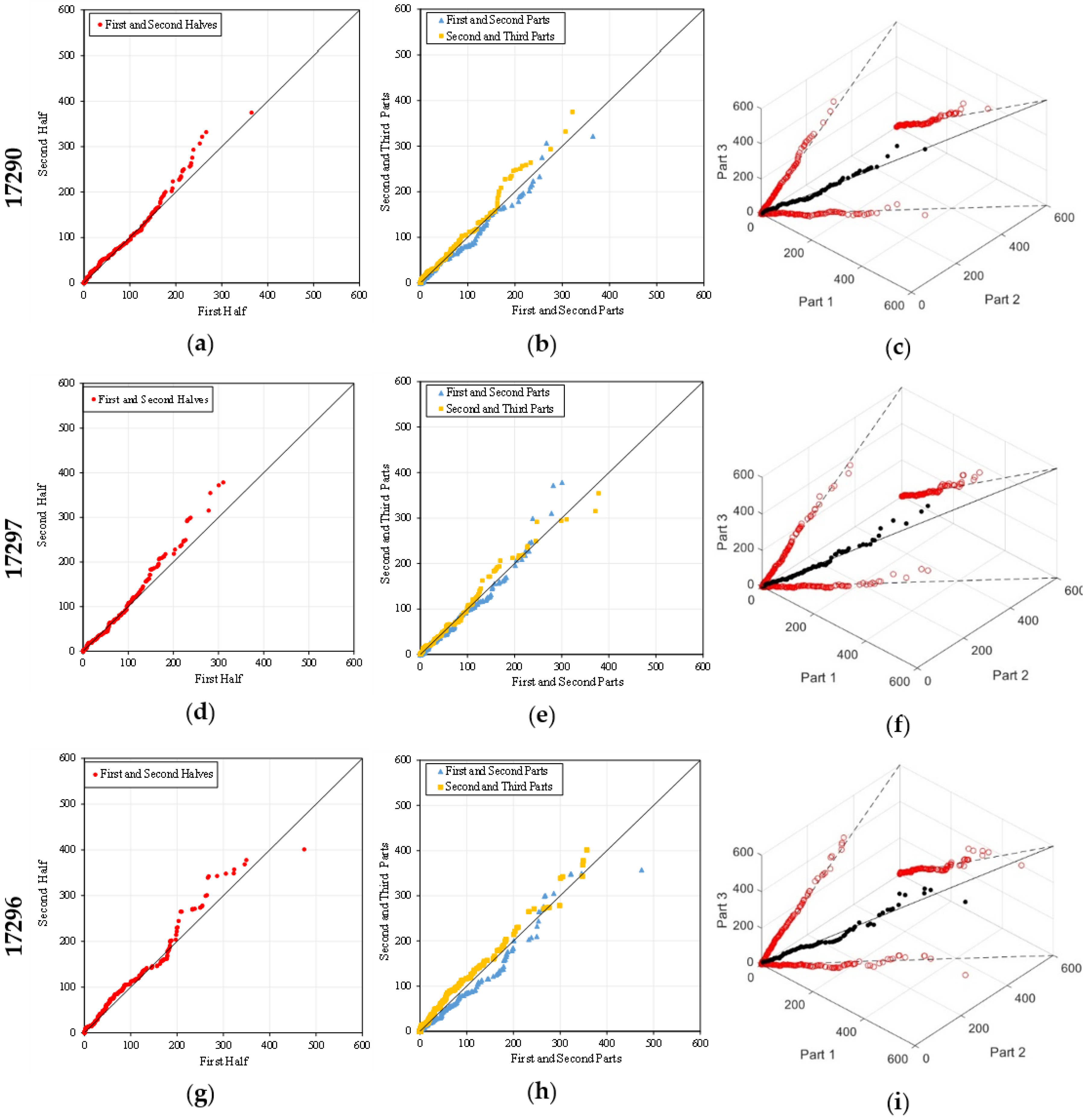
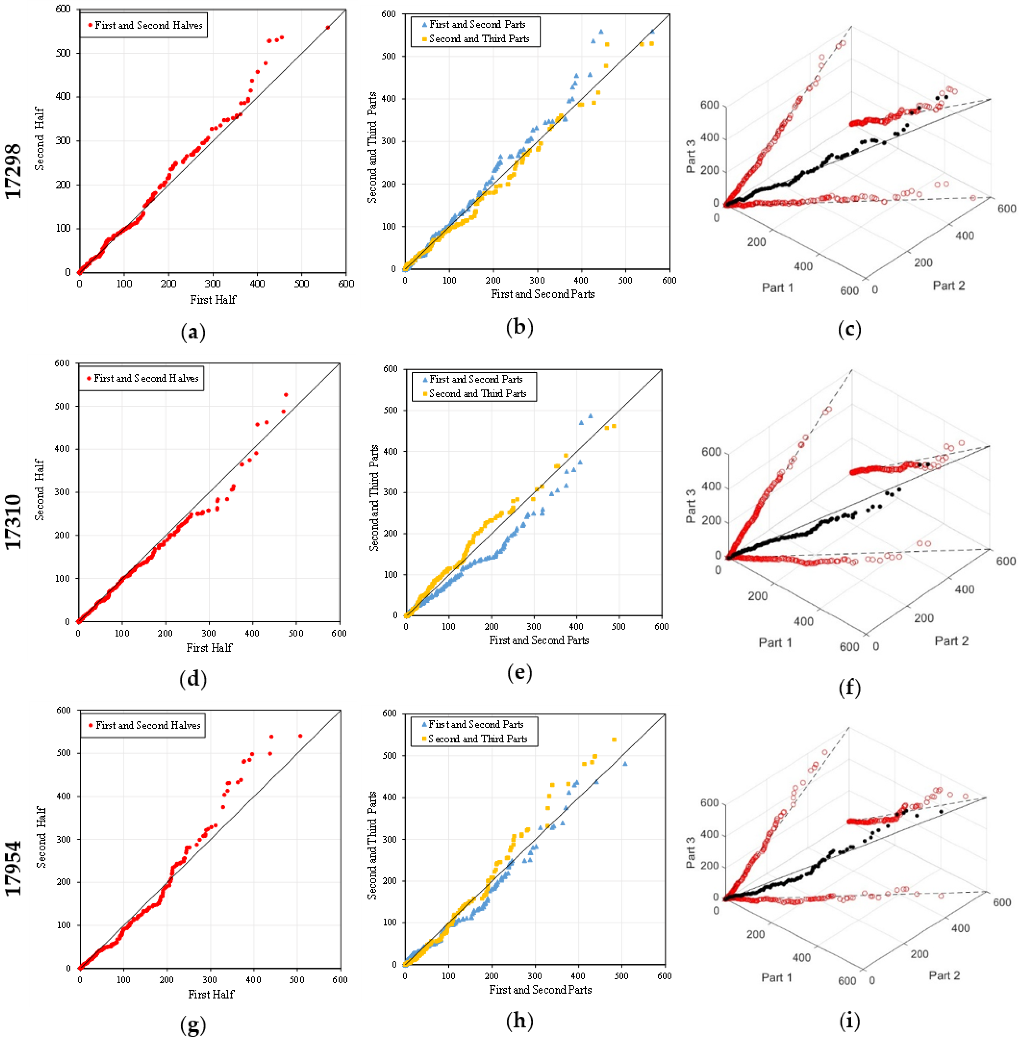
Figure 6 and Figure 7 illustrates two segments (1974–1997; 1998–2021) and three segments (similar to the MK and WT) of the ITA and 3D-ITA at six precipitation stations. More specifically, in the first column, the two segments are four 24 years (1974–1997) and one almost 24 years (1998–2021) and in the second column, three segments are implemented, and the third column provides the 3D-ITA to help visualize trend stabilities within each station. In Figure 6, the investigation of the first three stations (17290, 17297, and 17296) conveys both commonalities and differences in their long-term trend behavior. At station 17290, the results indicated a monotonic increase with no sample catching a decreasing period across any of the ITA visualizations; both the two-part and three-part division showed higher values in the second half of the 1960–2015 sampling period. The 3D-ITA visualization, understandably, supported this finding with scatters points clustering in close proximity to the 1:1:1 reference line, leading to the conclusion that monotonic increase was weakly stable.

Station 17297 revealed a non-monotonic pattern with erratic fluctuations. While some sub-periods showed short-term increases, the general trend showed irregularity and lacked systematic persistence. The ITA results showed switching between upward and static phases, while the 3D-ITA results demonstrated broad dispersion of points about the 1:1:1 line, representing an unstable trend structure. Thus, this station indicated an unstable non-monotonic behavior, rather than weakly stable or systematic upward behavior. Conversely, station 17296 also demonstrates an increasing trend, although the trend is non-monotonic. The three-period inspection elucidates alternating periods of weaker and stronger growth. In the 3D-ITA space, the data points deviate somewhat from the 1:1:1 line, showing some stability. Thus, while there is an overall increasing pattern, the nature of the pattern is less uniform than at station 17290, but more stable than at station 17297. Overall, the three stations show increasing trends, but the levels of stability are different: station 17290 demonstrates a stable monotonic increase, station 17297 shows weakly stable non-monotonic increase, and station 17296 reflects a moderately stable non-monotonic increase.

Evaluating the other three stations (17298, 17310, and 17954) indicated different trends in both direction and stability (Figure 7). Station 17298 showed a monotonic increase; on the contrary, the two-part plus three-part ITA divisions showed a no-trend in values in recent decades. The 3D-ITA plot also corroborated this finding, as most of the points were positioned relatively close to the 1:1:1 reference line, showing that there is moderate stability in this upward trend with only minor fluctuations in values. Therefore, station 17298 is one of the more stable stations included in the analysis.

In contrast, station 17310 shows a monotonic decrease. Both the comparisons of ITA and the separation of the comparisons into three periods produce systematically lower values towards the end of the record, indicating that the station is on a continuing decrease. The 3D-ITA shows similar behavior, with points moving below the reference line representing moderate-to-low stability in the decreasing pattern. Thus, 17310 makes an interesting distinction in that it is the only station showing a declining trend. Finally, station 17954 shows a non-monotonic increase. While the long-term trend is increasing, the ITA statistics show some substantial fluctuations across periods and the 3D-ITA distribution shows points more scattered from the 1:1:1 line. This indicates the station has had an increase overall while showing an increase with low stability and irregular growth compared with the other sites. Together, these three stations show a diverse set of behaviors: 17298 shows a stable monotonic increase, 17310 shows a declining monotonic change, and 17954 displays a non-monotonic increase with weak stability. In brief, analyses of the ITA and 3D-ITA demonstrate that the majority of stations (17290, 17296, 17297, 17298, and 17954) exhibit increasing patterns, but with varied stability. Among the increasing trends, 17290 and 17298 have more stable monotonic increases, 17296 and 17954 have non-monotonic increases with moderate to low stability, and 17297 exhibits the most unstable increasing trend. Station 17310, on the other hand, had a distinct monotonic decreasing trend.

4. Discussion

A comparison of the results obtained through the MK and WT methods indicated similarities as well as some differences, depending on the threshold applied. The MK and WT analyses indicated that the basin was generally stable at the 1% threshold, with no significant monotonic changes. The only exception to this finding was for Station 17296, which indicated a significant positive trend for the period of 1983–2012 from the WT analysis, but was not identified as statistically significant in the MK analysis. This is an important finding, as it indicates that the WT method is able to identify unique localized changes that did not show up in the MK method when it applied a more conservative approach. Given the 5% significance threshold, the differences between the two measures began to diverge a bit more. The MK measure still indicated no significant monotonic changes, while the WT, which had previously been conservative, began indicating additional signals of variability along the segment. In particular, the WT measured positive trends at Stations 17290 and 17296 for the period of 1983–2012, and a negative trend at Station 17310 during the period of 1974–2003. Overall, there does appear to be some indication that the WT method may be responding to shorter-term and sometimes more localized changes and variability, in contrast to the MK method, which tends to smooth out local variability and put a stronger emphasis on longer-term stability.

When assessing the results at the more lenient 10% threshold, the complexities of the outcomes increased again. MK identified only one significant monotonic trend, which was a positive trend at Station 17296 for the 1983–2012 period. Conversely, WT revealed a consistent suite of significant outcomes for the same station. These trends included positive trends at 1974–2003, 1983–2012, and 1992–2021, as well as the entire record. Moreover, WT echoed earlier evidence of a positive trend at Station 17290 (1983–2012) and a negative trend at Station 17310 (1974–2003), both of which were not shown with MK. Thus, the WT method was more sensitive to temporal variability, detecting instabilities that MK did not capture.

In summary, both tests show overall stability of the hydroclimatic series when assessed at moderate thresholds. Relaxing the thresholds showed localized spots of change in interest in the series. Of the stations with localized evidence of change, Station 17296 has the most dynamic evidence, alternating between a positive and negative signal across methods and sub-period, while Stations 17290 and 17310 provided secondary evidence of localized variability. The findings shown in the comparison indicate that MK is strong for monotonic change over long periods of time, while WT is a useful method for identifying subtle, or short-term change, which can be hydrologically significant. On the other hand, the WT is more sensitive to short-term variability, but this sensitivity may yield pseudo variations resulting from temporary extreme events or noise in data instead of fundamental long-term changes.

Investigating the role of ITA in this study has further improved our interpretive capability by separating monotonic, non-monotonic, and trendless conditions under one of the most appealing characteristics of the revisions to MT, namely the binomial either/or choice of MK and WT. However, it is the use of ITA, specifically the 3D-ITA extension, that added an invaluable measure specifically interrogating trend stability. As a demonstration of our key conclusions, the results were summarized in

Table 6. Summary of the trend and trend stability results.

Station	All Data (1974–2021)			Data for (1974–2003)			Data for (1992–2021)
	MK	WT	ITA	MK	WT	ITA	MK	WT	ITA
17290	No Trend	No Trend	NM+	No Trend	No Trend	NM−	No Trend	No Trend	NM+
17297	No Trend	No Trend	NM+	No Trend	No Trend	No Trend	No Trend	No Trend	NM+
17296	No Trend	No Trend	NM+	No Trend	No Trend	M−	No Trend	No Trend	NM+
17298	No Trend	No Trend	NM+	No Trend	No Trend	NM+	No Trend	No Trend	No Trend
17310	No Trend	No Trend	NM−	No Trend	M−	M−	No Trend	No Trend	M+
17954	No Trend	No Trend	NM+	No Trend	No Trend	NM−	No Trend	No Trend	NM+

M+: monotonic increase (consistent upward trend); M−: monotonic decrease (consistent downward trend); NM+: non-monotonic increase (fluctuating but generally upward pattern); NM−: non-monotonic decrease (fluctuating but generally downward pattern).

, where the illustration of instability reveals oscillatory yet non-monotonic behavior—indicating variance in temporal or structural dynamics that has largely eluded interpretation through MK and WT tests alone. As an example of findings highlighting instability, Station 17296 exhibited alternating non-monotonic positive signal patterns, or structure, and monotonic negative patterning in the same 2003–2021 sub-period—again, constantly oscillating with no ability of either MK or WT to inform about signal behavior. Similarly, Station 17310 demonstrated change, or signal instability, moving from monotonic decrease with weak trends in the period from 1974 to 2003 to monotonic increase in the period 1992–2021. In the example of stations where there was no trend (e.g., Stations 17290, 17297, 17298, and 17954), ITA revealed weak but unstable non-monotonic tendencies. The ability to differentiate the aspects of stable, unstable, and oscillatory patterns is particularly valuable in Mediterranean climates where high-frequency variability can dominate and distinguishing persistent shifts from temporary fluctuations can be crucial in scientific interpretations and management applications [13,14,16,19,24,36].

The current findings are importantly consistent with studies recently published in the same region. For example, Kesgin et al. [30] examined hydroclimatic variability along Türkiye’s southern coasts and revealed that MK often underestimated variability, and that ITA appropriately captured complex non-monotonic behavior. Consistent with their findings, the current study showed that WT allowed the recognition of complementary sensitivity to change on a localized scale, and that ITA and 3D-ITA revealed new insights into trend stability. Collectively, these approaches complement each other, and motivate an interpretive framework that ensures subtle but potentially important signals are not missed.

From a methodological standpoint, the MK test [3,4] has been well-established for decades as one of the more prevailing methods in hydrology, appearing to have greater strength in determining whether there is a monotonic trend over a longer time frame. Manifestly, the MK test appears to be less responsive to the weaker oscillations. This conservative response was measured in the current study, as the MK test frequently indicated that the process was stationary when variability existed in the data. These findings fit with previous research that argued the MK test lacks ability to detect shorter-term variability, especially in a Mediterranean climate [8,9]. In contrast, the WT method [22] considers difference without reordering the data, and therefore, is more responsive to any local changes or shorter-term oscillations. Overall, WTs were able to pull out subtle signals that were not captured in the MK method, thus providing a different perspective.

The results of this study are in line with recent works concerning the benefits of different non-parametric strategies in detecting hydroclimatic trends. Küçükerdem Öztürk et al. [25] demonstrated that the combination of MK and WT as well as newly developed graphical tests provides better sensitivity to minor or non-monotonic changes. Similarly, both Yüce et al. [26] and Akbaş et al. [27] established that ITA-based methods are capable of detecting oscillatory rainfall patterns that may not be highly detected by conventional tests. Overall, the present results were in agreement with those findings and demonstrate that the combination of MK, WT, and ITA can improve the reliability and interpretative rigor of precipitation trends in a changing climate.

Additionally, the variations across MK, WT, and ITA metrics can be partially attributed to the regional climatic and topographic influences over rainfall variability along Türkiye’s southern coastline. The region is described as being influenced by Mediterranean cyclones, the North Atlantic Oscillation (NAO), and air–sea interactions that influence moisture transport and convection. While positive NAO phases can be associated with reduced winter rainfall, negative NAO phases often lead to increased storminess and rainfall. Large-scale circulation differences in this type, when combined with steep coastal to mountain topographic gradients, may generate rainfall responses that are spatially heterogeneous. As a result, WT, which responds to short-lived variability, often captures transient oscillations and variability more so than MK, which emphasizes persistence and monotonic trends. The response to atmospheric circulation and terrain helps explain the observed differences in the magnitude and direction of trends for each method.

Moreover, the period of study coincides with a distinct period of global warming, when increasing air and sea-surface temperatures have led to changes in large-scale circulation and moisture transport in the Mediterranean region. One effect of these changes can be reduced temporal stability of rainfall trends by increasing interannual variability and altering storm tracks. For example, increasing sea-surface temperatures and extended dry periods can cause localized variability that can be associated with short-term instabilities detected by WT and ITA methods. Thus, the impacts of global warming likely represent an underlying driver of reduced persistence of regional precipitation regimes along Türkiye’s southern coasts.

Regarding computational efficiency, the MK test still provides the best time efficiency due to its simple rank-based pairwise comparisons, which makes it useful for long-term or large datasets. The WT method is slightly more computationally taxing but typically has more statistical power when using usual periods or small sample sizes. In contrast, ITA and particularly 3D-ITA require a greater amount of time predominantly due to the additional ranking step and different visualization of results. However, its trade-off is greater diagnostics into the stability of trends. Therefore, the combined use of these methods allows scalable and flexible application across datasets of varying temporal length and resolution.

While although the results provide helpful evidence regarding the stability of hydroclimatic trends, it is important to recognize several limitations. The analysis is based on data from only six meteorological stations, which could constrain spatial generalization of the results to the entire Mediterranean area. Although homogeneity and quality checks were thoroughly conducted, there could still be residual uncertainties in observational records and consistency of measurements. Further, methods involved in the analysis, specifically ITA and WT, are sensitive to data length and timeline choices, which could potentially affect interpretation of trend stability. External climate drivers, such as large-scale tele-connections or anthropogenic drivers, were not quantitatively modeled, and an explicit form of modeling could have strengthened future work. Addressing these factors in future analysis will assist in improving reliability and applicability of trend stability conclusions under varying climate.

In conclusion, the integration of MK, WT, and ITA with a combined approach is both methodologically sound and practically useful. While MK identifies sustained and long-term monotonic changes necessary for decisions regarding the function of infrastructure, WT identifies short-term variability to aid in risk management. ITA with an extension to 3D, in particular, offers a unique classification of trend stability (Table 6), fundamental in understanding hydroclimatic dynamics in high variance Mediterranean contexts. Therefore, the multi-method of approach adopted here provides solid footing for climate adaptation strategies, risk assessment, and resilience-building within water resource management. Furthermore, the findings pointed out here also have broader applicability to other parts of the Mediterranean regions beyond Türkiye. Because Mediterranean-type climate regimes have analogous regimes of precipitation and modes of variability, this analytical method implemented in this study can be readily applied to comparable cases in Southern Europe and North Africa including Spain, Italy, Greece, Morocco, Tunisia, and Algeria. Such cross-regional applicability enhances the value of trend stability analysis as a method for estimating hydroclimatic resilience and informing sustainable water management practices in different Mediterranean basins.

5. Conclusions

This study evaluated long-term rainfall variability on the southern coasts of Türkiye using three complementary non-parametric approaches: Mann-Kendall (MK), Wilcoxon Signed-Rank Test (WT), and Innovative Trend Analysis (ITA). The comparative review confirmed that MK presented a cautious view of long-term monotonic changes, which was generally not responsive enough to account for localized variations. In contrast, WT indicated localized fluctuations more readily and thus offered insights that complemented the MK findings across long-term trends. Importantly, the ITA, as well as its 3D version, provided an additional level of interpretation in that it not only recognized change direction but also identified stability of any trends convincing enough to warrant stability assessment. A few of the stations showed an oscillatory or unstable pattern that MK and WT would most probably miss, indicating the importance of trend persistence in hydroclimatic analyses to comparatively assess contextually whether trends are permanent compared to transient or fleeting. Generally, MK, WT, and ITA together gave a better account of rainfall variability. MK is obviously robust for detecting persistent trend over the long term, WT is highly sensitive to variability at local scales, and ITA helps to display stability as an additional aspect of analysis.

The findings of a trend stability analysis also provide actionable information that can facilitate the sustainable management of water resources. The identification of stable or unstable rainfall trends provides a foundation for decision-makers to engage in adaptive management around reservoir operations, irrigation scheduling, and preparing for drought. Specifically, stable increasing trends will encourage decision-makers to maximize storage and optimize irrigation practices, whereas unstable or decreasing trends encourage careful allocation of available resources, especially with regard to planning for drought. Understanding how to incorporate this type of information into management frameworks can help increase the adaptability and resilience of water systems in changing climates. Furthermore, the methodological framework and findings can be extended to other Mediterranean basins such as those in Spain, Italy, Greece, Morocco, Tunisia, and Algeria, which share similar climatic variability and water management challenges. This universality highlights the study’s contribution to regional-scale climate resilience and sustainability. Combined, these approaches provide methodological robustness that can be utilized for risk assessment, adaptation planning, and sustainable water resources management in regions characterized by variable rainfall patterns.

In addition, the proposed methods may be used in other areas of the Mediterranean climate zone as long as the research relies on long-term quality-controlled precipitation data. MK and WT tests can be applied provided that they have sufficient temporal stability in their dataset, while methods based on ITA require a substantial length of the dataset that reveals both stable and unstable trends. Applications can certainly be generalized to different climatic conditions, yet their capacity to yield reliable patterns may be compromised in environments characterized by few data points, or gaps in the data. Therefore, future applications should continue to consider elements of data completeness and climate variability in considering trends stability.