Abstract
This study applies the Life Cycle Assessment (LCA) to evaluate the environmental impacts of different types of road construction, including at-grade sections, trenches, embankments, viaducts, and tunnels. The functional unit used is 100 m, and system boundaries consider raw material extraction, transport, construction, and operation based on a 30-year lifetime. Impact categories considered are Global Warming Potential (GWP), Acidification Potential (AP), Eutrophication Potential (EP), Photochemical Ozone Creation Potential (POCP), and Human Toxicity Potential (HTP). Results show that tunnels generate the highest impacts during construction, particularly in terms of CO2eq and SO2eq, while operational impacts remain similar across all road types. A valuable consideration can be made on the “emissions equivalence” observed when the length of the at-grade road is approximately twice that of the tunnel, enhancing the importance of a “full view” of the impacts. In exploring mitigation strategies, the use of bottom ash from municipal solid waste incineration as an alternative material reduced GWP-related emissions by about 50%. While the existing literature tends to focus on individual types of infrastructure or specific materials, the following work proposes a systemic approach that links design choices to circular economy strategies, quantitatively demonstrating the potential for reducing environmental impacts using secondary materials.
1. Introduction
This study is finalized to conduct a Life Cycle Assessment (LCA) of different types of road sections. This analysis will be developed in accordance with ISO 14040 [1] and ISO 14044 [2] standards. The emission impacts of the various road sections will be compared considering the phases from raw material extraction to construction and the operational phase; the decommissioning phase is not considered. Often, during the design phase, there are no alternatives in road layouts, but sometimes several solutions can be considered: a typical example is a tunnel, and as an alternative, a route at ground level, which will result longer in terms of development. In these cases, the cheapest or fastest solution is often chosen, and aspects related to the impact of construction and the impact of use of the road type in time are often overlooked. Finally, with the aim of optimizing the use of resources in road construction, alternative building materials will be analyzed in order to identify solutions with a lower environmental impact. For the analysis, a software called InfraLCA v.1 (based on the ISO guidelines) was developed internally by the research group to be as specific as possible in pursuing the objectives of the study.
The main objective of this research fits within the context of the sustainability requirements outlined in the 2030 Agenda, with particular reference to target 9.1 to develop high-quality, reliable, sustainable, and resilient infrastructure, target 9.4 to improve infrastructure and sustainably reconfigure industries by 2030, and target 11.2 to provide access to safe, sustainable, and accessible transport systems for all and improve road safety. With respect to target 9.1, the comparative LCA results show how different roadway cross-sections can affect environmental performance. For example, the construction phase of a 100 m at-grade road releases an emission of 729 t CO2eq, whereas for a 100 m tunnel the emissions reach 3914 t CO2eq. This means that the same emissions of CO2 for the construction of a tunnel are the same of those emitted for the realization of approximately 534 m of at-grade road. This quantification enables infrastructure planners to select configurations that are more environmentally efficient and resilient, promoting sustainable infrastructure design consistent with SDG 9.1.
Concerning target 9.4, the research demonstrates that substituting conventional raw materials with industrial by-products—specifically, bottom ash from municipal solid waste incineration—can lead to an approximate 50% reduction in CO2, SO2, and NOX emissions during the construction phase. This measurable improvement illustrates how industrial symbiosis and material recycling can significantly enhance the environmental performance of the construction sector, contributing directly to the sustainable reconfiguration of industrial processes envisioned by SDG 9.4.
Finally, in relation to target 11.2, the study integrates both short-term (construction) and long-term (operation) emissions over a 30-year lifetime. This shows that overall CO2 emissions balance between road types can be obtained with different lengths of the route allowing the possibility to choose the road route according to environmental and sustainable considerations. This integrated, life-cycle perspective demonstrates how sustainable infrastructure planning can optimize both mobility efficiency and environmental impact over time, supporting the transition toward safe, accessible, and low-emission transport systems as promoted by SDG 11.2.
The impact categories considered in the analysis are Global Warming Potential (GWP), Acidification Potential (AP), Eutrophication Potential (EP), Photochemical Ozone Creation Potential (POCP), and Human Toxicity Potential (HTP). These environmental categories were selected as they are the most relevant in terms of the pollutants emitted as well as they are the most considered in several articles on similar topics [3,4,5,6]. The functional unit is chosen equal to 100 m of road infrastructure, and the system boundaries include all construction phases—from raw material extraction and transport to the operation of the road—assuming a useful life of 30 years. Road construction, not only in terms of defining its impact, but also in relation to economic growth and models for monitoring construction, has been addressed by several authors [7,8,9,10,11,12].
The following study is based on the application of the LCA methodology, which is widely used in many studies [4,13,14,15] and on different topics [16,17,18]. One example is Trunzo’s study [19], which shows that life cycle assessment reveals that almost half of the environmental impact of a provincial road occurs during the construction phase. The use of eco-friendly design, low-impact materials, and recycled resources can significantly reduce this impact. However, Trunzo’s analysis describes a single case study, without standardized comparative evaluation or exploration of alternative materials, whereas this study develops a parametric comparative model based on a homogeneous functional unit (100 m), allowing direct comparisons and introducing mitigation strategies based on the circular economy. The study of Ulla-Maija Mroueh [20] found that material production and transport are the main sources of environmental impact in road construction. Bitumen and cement production, material crushing, and transport are the most energy-intensive stages. However, it does not analyze the complete life cycle or compare different types of road sections (cut, embankment, tunnel, viaduct, etc.). On the contrary, this study updates the approach by introducing a more comprehensive LCA model (“cradle-to-operation”), with broader system boundaries and comparative analysis between different types of infrastructure. Furthermore, the link between road morphology and impacts is quantified. Using secondary materials like coal ash or crushed concrete can reduce the use of natural resources, even if their leaching behavior should be carefully assessed. The LCA study performed by Jullien [21] shows that maintenance accounts for about one-third of the total environmental impact over a 30-year road life. Both construction and maintenance significantly affect environmental indicators, highlighting the need for full life-cycle-based design to reduce environmental loads. The study anyway does not include different geometric configurations of infrastructure (e.g., tunnels vs. at-grade roads) nor does it evaluate useful life and operational emissions in an integrated manner. In contrast, our study adds a quantitative comparison between road morphologies and a combined construction-use analysis over 30 years, showing for the first time an environmental equivalence threshold (around 194%) between tunnels and at-grade roads. The LCA case study at Heathrow Terminal-5 by Huang [5] shows that hot mix asphalt and bitumen production are the most energy-intensive processes. Using recycled materials like glass, IBA (Incinerator Bottom Ash), and RAP (Recycled Asphalt Pavement) the impacts can be reduced. However, the comparison between recycled and traditional materials is limited to surface paving and, without extending the analysis to the entire infrastructure characteristic of the road type. Again this article extends the application of alternative materials to the entire road realization, quantitatively demonstrating how the use of bottom ash affects not only the paving but also the overall CO2 and SO2eq balance of the infrastructure. The review of [22] highlights that using recycled construction and demolition (C&D) waste in pavements can reduce landfill use and environmental damage from natural aggregate extraction. LCA shows environmental benefits, supporting the use of C&D waste to promote sustainable and low-waste road construction.
A comparative analysis of different road sections has been little addressed in a systematic and multidisciplinary manner in the existing literature. From an innovative point of view, an integrated design methodology is proposed able to take global environmental impacts into account in a predictive manner in the road section/route definition phase. So this study is among the first to integrate construction and operational LCA of various road geometries using a consistent 100 m functional unit.
2. Materials and Methods
This study uses LCA methodology to determine the impacts associated with the construction and operation of various road types. This method is cutting-edge and highly relevant to the analysis, as it is a tool for analyzing the environmental implications of a product throughout all stages of its life cycle, i.e., raw material extraction, material processing, product assembly, use, and end-of-life scenario [23,24]. LCA follows international guidelines (ISO 14040 and ISO 14044), which guarantee scientific rigor and comparability of results. It consists of four phases [25,26,27]: definition of the scope and boundaries of the system, which is extremely important for understanding the extent of the analysis; definition of the system inventory and therefore the inflows and outflows from the system itself; definition of the impacts based on the different environmental categories considered relevant to the study carried out (a further strength of LCA is that it allows for multi-category quantification); and finally, interpretation of the results.
The use of LCA in this study not only allows for a quantitative assessment of environmental impacts but also identifies critical points in the process (hotspots) and compares different design or management alternatives. The application of this method in the field of road embankment construction is also innovative, as it provides scientific data and results in a field of research that has yet to be fully explored.
2.1. Goal and Scope Definition
This study stems from the need to quantify the benefits and potential impacts on the environment and humans associated with the entire life cycle, from the extraction and production of raw materials to the operational phase, of various types of road sections. This objective therefore includes quantifying the impact of various infrastructures, comparing traditional raw materials with alternative raw materials, and finally comparing the impact of different types of road sections with others of different lengths in order to determine which solutions are most cost-effective in terms of environmental emissions.
2.2. Functional Unit (F.U.)
The functional unit is an important choice in an LCA study, as the impacts refer to it. Several studies have considered a specific length of road, usually 1 km as the functional unit [28,29,30,31], while others have considered an area of road, usually 1 m2 [32]. The following study considers 100 m of road section laid as a functional unit. This unit was chosen because tunnels or viaducts are very often less than 1 km long. In such cases, the procedure could not be easily applied to all routes. In any case the results can be considered directly proportional to the chosen length.
2.3. System Boundaries
The boundaries of the system determine the input and output flows and, consequently, the impacts considered. It is therefore extremely important to define these boundaries in an LCA study in order to understand exactly what the impact results refer to [33]. The system boundaries considered in this study include the extraction of raw materials as well as the processing and production of materials used for the construction of road embankments, to be referred to within the conversion factors considered (Figure 1). Transport for supply and waste disposal was also considered. Finally, in addition to construction, the operational phase was considered, assuming a useful life of 30 years for the road section.
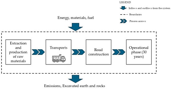
Figure 1.
Boundaries of the system.
2.4. Life Cycle Inventory (LCI)
The input and output data considered in the following analysis are, respectively, consumption of raw materials and energy (thermal or electrical) as inputs, and waste and atmospheric emissions as outputs. Raw materials are included in the materials used to construct road embankments and therefore consist of concrete, bituminous conglomerate, aggregates, and steel. The quantities required to construct 100 m of road are shown in Table 1. Figure 2 shows the dimensions to which all road types refer.

Table 1.
Quantities of material (m3) required for 100 m of road with different types of cross-sections.
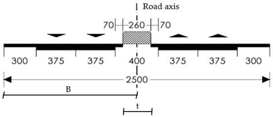
Figure 2.
Category A Motorway—basic solution with 2 + 2 lanes (data in centimeters).
For electricity consumption associated with the operational phase (30 years), an estimate of consumption relating to electrical systems and vehicle traffic was considered, based on estimated Average Daily Traffic (ADT) and using the consumption factors of the COPERT V calculation software (COPERT version 5.8.1—September 2024), equal to 1.31 MJ/km per vehicle. As regards thermal energy, during the construction phase its consumption is associated with the fuel used to power all vehicles involved in the extraction, production, and transport of materials, as well as in the construction of the road section. In this case, based on vehicle activity in terms of meters traveled, an average consumption of 25 L per 100 km was assumed from experienced works of IRIDE; or, regarding the fuel required for motor vehicle traffic during the operational phase, based on the project’s ADT and the fleet of operational vehicles, a consumption of 8 L per 100 km has been hypothesized as an average value based on previous work by IRIDE. Regarding the materials produced for the construction of the work to be delivered outside the construction site, the assumed quantities are shown in Table 2, calculated on the basis of the geometric data of the road section and on the basis of the excavations for viaducts and tunnels examined in this case study.
Table 2.
Quantity of materials (m3) to be delivered outside the construction site.
For the at-grade road section, road embankment, and tunnel, an excavation depth of 0.40 m was assumed for the topsoil stripping. Finally, regarding atmospheric emissions produced by the activities, processes, and machinery involved in the life cycle of the study, the following assumptions were made:
- –
- Emissions from construction site vehicles: calculated based on the activities in terms of hours and type of vehicle, and using emission factors from tables A9-8 of the 1993 American Off-road Mobile Source Emission Factors Database;
- –
- Raw material emissions: calculated based on the quantities of materials or raw materials. The conversion factor for concrete is equal to 290 kg CO2/m3 (Ecoinvent, ICE Database v. 3.9, IPCC 2019) while for steel it indicates values of 1.65 kg CO2 per kilogram of finished product [34];
- –
- Operational traffic emissions: estimated using average emission factors obtained from the COPERT V calculation model, expressed in g/km per vehicle; in particular, estimates were made for particulate matter (PM10) equal to 0.03 g/km × vehicle, for nitrogen oxides (NOX) equal to 0.41 g/km × vehicle, for carbon monoxide (CO) at 0.66 g/km × vehicle, for methane (CH4) at 0.01 g/km × vehicle, for sulfur oxides (SOX) at 0.01 g/km × vehicle, and for carbon dioxide (CO2) at 229.17 g/km × vehicle;
- –
- Electricity consumption emissions: estimated using ISPRA emission factors [35], which indicate 400.4 g CO2/kWh.
There are generally three types of road pavements, consisting of bituminous conglomerate (BC), granular mix (GM), concrete (for rigid pavements), and cement mix (CM). This study considers motorways as a type of road, therefore, traditional flexible paving is generally preferred, consisting of layers of bituminous conglomerate superimposed on others in granular mix resting on a sub-base with good bearing capacity. The standard dimensions of this type of road, with a basic two-plus-two lane configuration, are shown in Figure 2.
In this specific case, reference was made to an average configuration, i.e., with a resilient modulus of the subgrade equal to 90 N/mm2 and several commercial vehicles passage equal to 10,000,000. The thicknesses used in this study are wearing course 6 cm; binder course 7 cm, base course 22 cm, and sub-base course 15 cm, as reported in Figure 3.
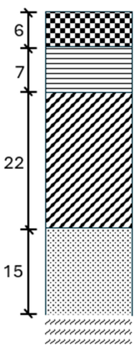
Figure 3.
Road sub-layer thicknesses (cm) used in this study.
2.4.1. Road Sections
In this study, various road sections were analyzed, some of which were assumed with different elevations. In particular, the viaduct was divided into three altitude categories: “high”, characterized by a height of 30 m; “medium”, with a height of 20 m; and “low”, with a height of 10 m. Similarly, the road embankment and road trench sections were classified into three altitude levels: “high”, with a height of 15 m; “medium”, with a height of 10 m; and “low”, with a height of 5 m.
The sections used in the LCA study are shown in Figure 4, Figure 5 and Figure 6, with the input data relevant for modeling in Table 3, Table 4 and Table 5: ground level section; high, medium, and low embankment sections; high, medium, and low cutting sections; high, medium, and low viaducts; natural–traditional tunnels.
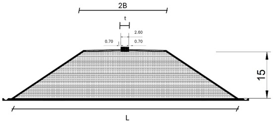
Figure 4.
Modeled section of a high road embankment (m).
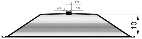
Figure 5.
Modeled section of a medium road embankment (m).
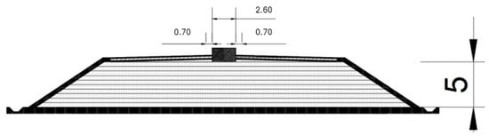
Figure 6.
Modeled section of a low road embankment (m).
Table 3.
Road superstructure data in relation to the road embankment.
Table 4.
Road body data in relation to the road embankment.
Table 5.
Road superstructure data in relation to the road trench.
Figure 7, Figure 8 and Figure 9 show the data relating to the road trench. Table 5 and Table 6 show the data relating to the construction of the road superstructure of the road trench and the excavation of the road trench itself.
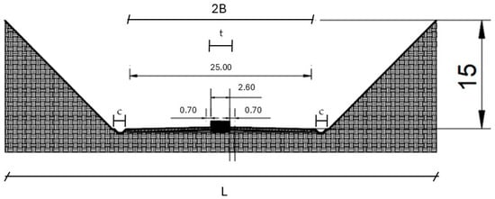
Figure 7.
Modeled section of a high road trench (m).
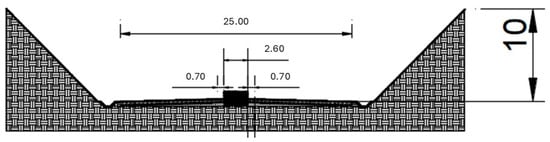
Figure 8.
Modeled section of a medium road trench (m).
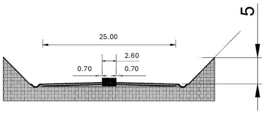
Figure 9.
Modeled section of a low road trench (m).
Table 6.
Data relating to the excavation of the road trench.
Figure 10, Figure 11 and Figure 12 show the sections of the different types of viaducts considered with their relative measurements. Table 7 and Table 8 show the data relating to the quantities of materials used to build the single viaduct and its characteristics, respectively.
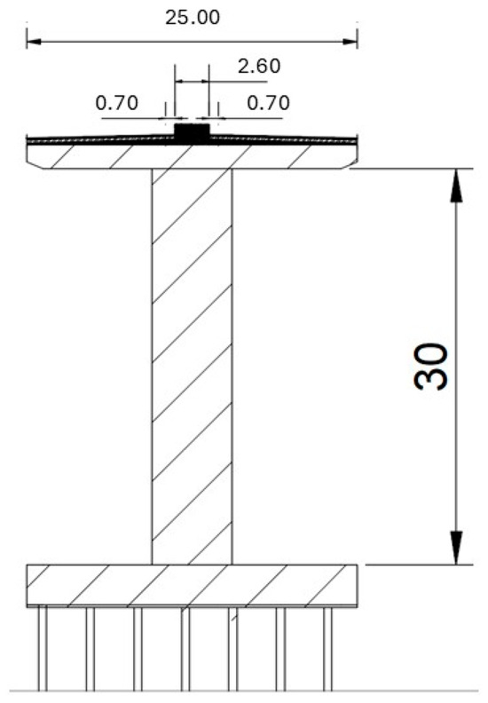
Figure 10.
Section of a high viaduct (m).
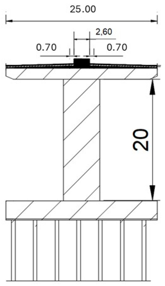
Figure 11.
Section of a medium viaduct (m).
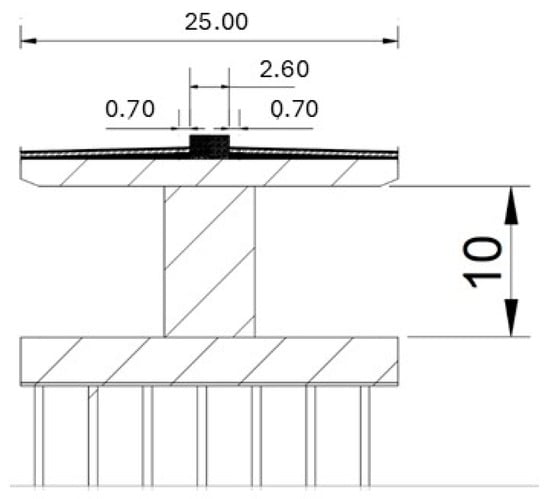
Figure 12.
Section of a low viaduct (m).
Table 7.
Road superstructure data in relation to the viaduct.
Table 8.
Data relating to the type of the viaduct.
Figure 13 shows the representation of a natural tunnel with traditional excavation, while Table 9 and Table 10 show the quantities of material used to construct the tunnel and its characteristics.
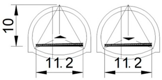
Figure 13.
Modeled section of a natural tunnel in traditional excavation for the two directions—typical section of the intrados (m).
Table 9.
Road superstructure data in relation to the tunnel.
Table 10.
Data relating to the tunnel.
When designing the various road sections, consideration was also given to the side gutters, two of which were placed on both side of the road and chosen with a “French-style” corrugation, and the guardrails, which were placed at the edges of the two carriageways, for a total of four.
The sections of both elements were calculated based on technical data sheets, which are shown in Figure 14 and Figure 15.
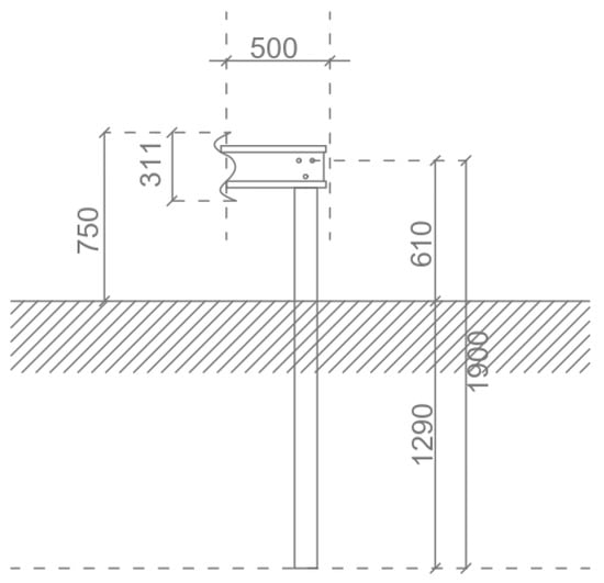
Figure 14.
Guardrail section from technical data sheet (mm).
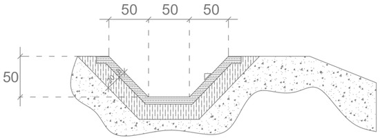
Figure 15.
Section of a French-style curb, from technical data sheet (cm).
The LCA study also considered the quantities of concrete and steel required for the installation of the aforementioned structures. The quantities of the various materials required to produce the road package section alone are therefore reported below (Table 11). Bituminous conglomerate, aggregates, steel, and concrete were considered. These quantities consider both the layers formed by asphalt concrete and aggregates and those composed of granular mix alone.
Table 11.
Quantity of materials required to produce the road package per functional unit.
The composition of the asphalt concrete and aggregates used is shown in Table 12.
Table 12.
Composition of materials.
It should be noted that a bitumen percentage of 4% was used, being the average range typically used in road paving construction between 4% and 6%.
2.4.2. Transport and Construction Equipment
The number and type of vehicles required at all stages of the life cycle analysis were provided by ANAS S.p.A. (the Italian state-owned company that manages and maintains the national road and motorway network), which supplied data on the vehicles required and actual daily production regarding the handling of materials by machinery, based on workers’ shifts. By also assuming a percentage of vehicle utilization, it was possible to calculate the number of operating hours required for each machine to complete the road section in question.
Regarding the emission factors for each vehicle and for each pollutant studied, Tables A9-8 of the 1993 American Off-road Mobile Source Emission Factors Manual, which provide a methodology and emission factors for calculating emissions from off-road mobile sources such as tractors, dozers, graders, etc., were used as references. The use of this methodology requires relatively detailed knowledge of the types of equipment that may be used as part of a proposed project. The composite off-road emission factors were derived based on equipment category (tractor, dozer, bulldozer, etc.), average fleet composition for each year through 2020, and vehicle population (number) in each equipment category by rated power and load factor. Daily emissions are calculated as reported in Formula (1).
where E is the emission in pounds per day; n is the number of pieces of equipment in a specified equipment category; H are the hours per day of equipment operation; EF is the off-road mobile source emission factor for equipment category or equipment category based on power in pounds per hour. In this specific case, emission factors for the year 2024 were used.
E = n × H × EF
2.4.3. Phase 1: Extraction and Production of Materials
For the extraction of raw materials, i.e., basic components of steel, concrete, asphalt concrete, aggregates, and earth and rocks (the latter exclusively for the supply of the road embankment section), a medium-power excavator with 175 hp and a productivity of 90 m3/h (calculated assuming a bucket capacity of 0.5 m3) was considered. Based on these assumptions, the total number of hours of excavator operation required to extract the raw materials needed to construct the following road sections is shown in Table 13.
Table 13.
Hours of excavator operation required to extract the raw materials for each road section.
The estimation of emissions to produce materials was limited to the quantification of carbon dioxide equivalent by various databases. Table 14 shows the emission indicator values for bituminous conglomerate and aggregates.
Table 14.
Emission indicators for the production of raw materials from various databases.
Regarding the emission values considered for bituminous conglomerate and aggregates, the average value between those of Table 14 was chosen in the input data, as follows: bituminous conglomerate equal to 20.1 kg CO2eq/ton and aggregates equal to 2.5 kg CO2eq/ton.
2.4.4. Phase 2: Transport
To define emissions relating to the transport phase of materials, a few assumptions were made, seeking to consider situations that were as realistic as possible (Table 15).
Table 15.
Assumption for defining emissions relating to the transport phase of materials.
Based on these assumptions, the number of trips required to transport all raw materials was calculated for each road section. From this, assuming the travelled distance, the total kilometers traveled by the truck were calculated, and then the number of hours required based on the assumed speed. The kilograms of diesel fuel required and the mass of pollutants due to emissions were then calculated.
2.4.5. Phase 3: Construction
In order to calculate the emissions of pollutants into the atmosphere during the entire construction phase of the different road sections, a package of equipment necessary for the operations was configured, depending on the section, for excavation works—earthworks—topsoil stripping; bituminous paving; construction of the elevation structure; construction of the foundation structure; pre-consolidation; first and second phase coatings; construction of road embankments. Reference was made to the packages provided by ANAS S.p.A (Rome, Italy). For each road section, therefore, the specific operations used for the road section, actual daily volume of material produced, percentage of use of each vehicle, and duration of work shift (8 h) were defined.
Regarding the actual daily production of material, reference was made to the theoretical daily production, which was corrected by various factors, considering the length of the week, unfavorable events, and any double shifts. These factors, derived from technical data used in Italy for road construction, are the corrective factor for a week length equal to 0.86, the correction factor for adverse events equal to 0.9, and the correction factor for double shifts equal to 0.81. Based on the amount of material to be processed, the total operating time of each piece of construction equipment for each construction phase was defined. For the tunnel, an estimate was made of the meters of work constructed in a day, which in this case was equal to 2 m/day (from experienced works of IRIDE). An hourly fuel consumption of 8 L/h was also assumed for the construction equipment in order to estimate the total quantity.
For the laying of the road surface, topsoil stripping is planned for each section under study, except for the road trench section and the viaduct. This operation consists of removing the active surface layer of the soil, which is richer in organic matter and vegetation, to work in a more inert area. This practice is carried out for the preparation and levelling of the soil and weed control. In this study, the excavation was assumed to be 0.40 m deep and as wide as the road—25 m. The total volume of soil to be removed will therefore be 1000 m3 per 100 m of road (functional unit).
The number of hours required to excavate this volume of soil was calculated using a medium-power excavator, 175 hp, with a productivity of 90 m3/h (calculated assuming a bucket capacity of 0.5 m3), obtained from a standard technical data sheet. The excavator must therefore operate for approximately 9 h to excavate 1000 m3 of soil in the road sections where the subgrade phase is planned.
2.4.6. Phase 4: Operational Phase
For the operational phase along the 100 m section of road, regardless of the type of road section, a useful life of the infrastructure of 30 years was considered. For the calculations, the maintenance phases were not considered; this was possible due to the long times between the maintenance periods of the paving (5–7 years for at-grave roads and 10–20 years for the remaining structures) that give not comparable values of CO2 production with those of the construction and operational phase. To determine the Average Daily Traffic (ADT) for the infrastructure in question, data on annual traffic volumes on Italian motorways published by ANAS S.p.A. for the year 2023 were consulted. The analysis involved calculating the arithmetic mean of the Average Daily Traffic Volumes (ADTVs), obtained by dividing the annual traffic volumes by the number of days of measurement. This procedure was applied separately to light and heavy vehicle categories. Following the calculations described above, an ADT of 12,550 vehicles/day was defined, with a breakdown of 12,000 light vehicles (corresponding to 95.6% of total traffic) and 550 heavy vehicles (equal to 4.4% of total traffic). Keeping this percentage ratio between heavy and light vehicles constant, the analysis considered a 1% annual increase in ADT over the period established for the operational phase, i.e., 30 years.
A further analysis was also carried out to define the composition of the vehicle fleet in terms of fuel type, distinguishing between petrol vehicles, diesel vehicles, and electric vehicles (BEVs). In line with the transport sector’s emission reduction targets, as outlined in the Integrated National Energy and Climate Plan (PNIEC), the growth in the share of electric vehicles (BEVs) over the useful life of the infrastructure was estimated. The projection was made by analyzing historical growth trends, assuming a linear trend. This analysis showed an estimated increase in the share of electric vehicles of 21% over 30 years (Figure 16 and Figure 17).
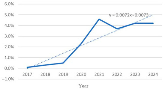
Figure 16.
Percentage of electric cars in Italy 2017–2024 (the dotted line represents the interpolated data, while the solid line represents the actual data).
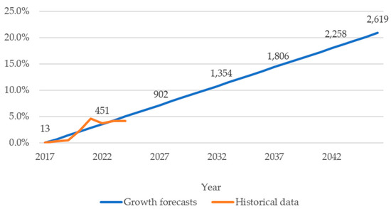
Figure 17.
Forecasts for growth in the percentage of electric cars in Italy over 30 years (2017–2047) based on realistic data (2017–2024)—the data labels represent the number of electric vehicles present in that year.
This study therefore considered ADT to be constant throughout the useful life, a linear increase in electric cars based on historical data, and a number of diesel cars equal to 40% of petrol cars. The energy mix for producing one kWh in Italy was assumed to be constant at 0.2572 kgCO2/kWh of electricity. For internal combustion engines, an emission factor in g/km × vehicle was associated, differentiated for light and heavy vehicles, from which the total emissions after 30 years of each pollutant studied were derived. Finally, fuel consumption for internal combustion engines was assumed to be 7 L/100 km for light vehicles and 30 L/100 km for heavy vehicles. A geometric mean was applied to obtain an equivalent consumption to be used for each petrol and diesel vehicle. This value was found to be 8 L/100 km. Table 16 shows the ADT data for light and heavy vehicles, while Table 17 shows the emission factors.
Table 16.
Average Daily Traffic (ADT) on Italian motorways published by ANAS S.p.A. for the year 2023.
Table 17.
Emission indicators to produce raw materials from various databases.
2.5. Life Cycle Impact Assessment (LCIA)
For the purposes of this study, impact factors imported from the international CML-IA Baseline database were used. Developed by the Centre for Environmental Sciences at Leiden University (CML), this methodology has established itself as an international benchmark. This methodology focuses on assessing environmental impacts at the “midpoint”, i.e., the intermediate points in the cause-effect chain between emissions and final impacts. This approach allows for greater transparency and a better understanding of the impact mechanisms. Furthermore, it is based on scientific data and established models, ensuring high reliability and robustness of results and finally, the CML-IA baseline is designed to be applied to a wide range of contexts and sectors, offering flexibility in the choice of parameters and indicators. For each environmental category, the CML-IA baseline provides characterization factors that enable the conversion of life cycle inventory (LCI) data into impact indicators. A “hierarchist” (H) approach was considered, i.e., with a time horizon of 100 years.
The impact categories considered in the analysis are Global Warming Potential (GWP—kgCO2eq), Acidification Potential (AP—kgSO2eq), Eutrophication Potential (EP—kgPO4eq), Photochemical Ozone Creation Potential (POCP—kgC2H4eq), and Human Toxicity Potential (HTP—kg1,4-DBeq).
3. Results
The results for the first three phases considered in the study are shown in Figure 18, Figure 19, Figure 20, Figure 21 and Figure 22 for GWP, AP, EP, POCP, and HTP, respectively. With regard to Phase 4, which in terms of values is the same for all road sections, it has been considered separately from the other phases to graphically appreciate the various intervals, since the latter is approximately one order of magnitude higher than the other phases. The data relating to this last phase are shown in Table 18.
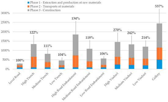
Figure 18.
GWP [ton CO2eq—100 years] regarding Phases 1, 2, and 3 normalized to the at-grade road (100%).
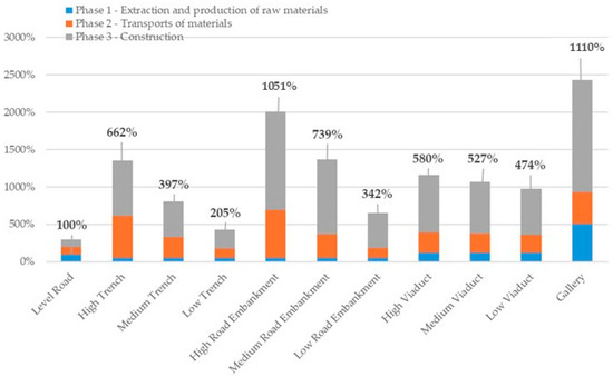
Figure 19.
AP [kg SO2eq] regarding Phases 1, 2, and 3 normalized to the at-grade road (100%).
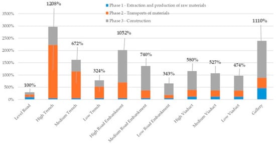
Figure 20.
EP [kg PO4eq] regarding Phases 1, 2, and 3 normalized to the at-grade road (100%).
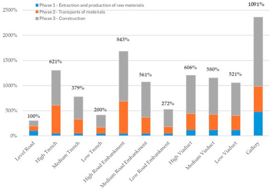
Figure 21.
POCP [kg C2H4eq] regarding Phases 1, 2, and 3 normalized to the at-grade road (100%).
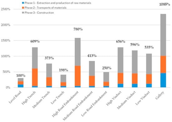
Figure 22.
HTP (c, np) [kg 1,4-DBeq] regarding Phases 1, 2, and 3 normalized to the at-grade road (100%).
Table 18.
Impact values of the different environmental categories chosen for the operational phase (Phase 4) considering an annual percentage increase of 1% in ADT.
From the data shown in the graphs above, it is possible to define the most significant value obtained from the point of view of environmental and human health impacts as that relating to GWP.
4. Discussion
The contribution to climate change is not uniform across the different phases. The result, in terms of tons of CO2eq, is summarized in Table 19.
Table 19.
GWP for different road sections.
Looking at the global warming values obtained, the phases with the greatest impact in terms of climate change are those related to the extraction and production of materials (Phase 1) and the operational phase (Phase 4). However, in the case of the extraction and production of materials, these emissions are not directly related to the construction and operation of the road sections studied, but rather to the extraction and processing of raw materials (i.e., steelworks and cement factories).
As regards the operational phase, it is possible to hypothesize that in the future, thanks to targeted measures to adapt transport methods, user habits could change and reductions in ADT could be achieved, bringing to a reduction CO2 emissions. Furthermore, growing global interest in the development of “green” technologies could accelerate the transition to vehicles with less impact and greater sustainability in terms of emissions.
The comparison of the results obtained in this study with the data reported in the existing literature is here reported. The GWP values obtained for at-grade road sections (about 729 ton CO2eq/F.U.) are higher than those reported by Moretti et al. (2018) [6] for urban and extra-urban roads (3500–5000 ton CO2eq/km). This difference is mainly attributable to the more complex structural configuration of highway-type sections and the inclusion of operational emissions over a 30-year lifetime. Nevertheless, the relative reduction achieved through the use of bottom ash (about 50%) is consistent with the mitigation potential highlighted in Moretti’s findings.
Moreover, the results of this study are consistent with those reported by Trunzo et al. (2019) [19], who found GWP values between 3000 and 8000 ton CO2eq/km for road infrastructures including tunnels and viaducts. The higher values obtained in this study (about 729 ton CO2eq/F.U. for at-grade roads and 3914 ton CO2eq/F.U. for tunnels) mainly reflect the more complex highway configuration and the inclusion of operational emissions. Both studies confirm that tunnels and viaducts generate several times higher impacts than at-grade roads, reinforcing the importance of design-stage environmental optimization.
Finally, with regard to the study conducted by Jullien et al. (2014) [21] comparing motorway pavement maintenance strategies, the following results are reported: the initial construction phase has an impact between 3000 and 4000 ton CO2eq/km; the maintenance produces around 1000–1500 t CO2eq/km. Therefore, considering construction alone, the values in this study are comparable to those reported by Jullien, although higher because the model proposed in this case study includes more complex structures and more materials (concrete, steel, earth).
4.1. Comparative CO2 Impact
With further analysis, a detailed comparison was made between an at-grade road section and a tunnel, with the primary objective of quantifying the difference in CO2 emissions between the two configurations. The preliminary results of the LCA, relating to the initial stages of the life cycle (from Phase 1 to Phase 3), show lower value in terms of emissions for the at-grade road section compared to the tunnel. Thus, 100 m of open road generates 729.0 ton CO2eq, while the same length of tunnel produces 3914 ton CO2eq. It follows that the emissions for the realization of 100 m of tunnel are equivalent to those produced for the realization of 534 m of at-grade road, as shown in Figure 23 (the figure supports direct comparison of scenarios with the same associated emissions).
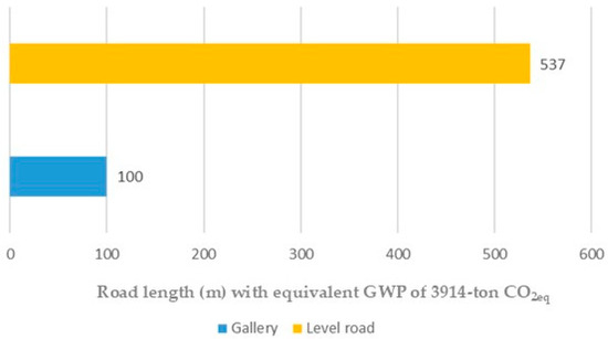
Figure 23.
Comparison of tunnel length (100 m) and at-grade road length (537 m) with equivalent GWP of 3914 t CO2eq.
It can therefore be concluded that in the short term, i.e., considering only the life cycle of the project up to its construction (Phase 3), the at-grade road section is preferable, with a reduction in emissions of up to 81.4% compared to the tunnel. However, it is also essential to consider the medium and long term, which in this case means considering the number of emissions at the end of the project’s useful life, due to a longer road traveled by vehicles. This consideration can be forwarded using the simple concept that 100 m of tunnel could be substituted, in terms of impacts, with 537 m of at-grade road. This is a design evaluation easy to encounter in reality because a tunnel can be used to cross an obstacle with a lower length of the path while the at-grade road is necessarily designed with a longer distance to avoid the obstacle. So, the comparison could be faced considering two possible solutions: 100 m of tunnel or 537 m of at-grade road without considering slopes. The comparison of the impacts shows the initial advantage of the at-grade road in the construction, but as shown in Figure 23, the higher length of the at-grade road has, as a consequence, higher emissions in the work life.
In fact, an analysis that includes the 30-year operating phase (Phase 4) shows that a 537 m at-grade road emits almost three times (277%) the amount of CO2 compared to a 100 m tunnel. Considering the above results, the equivalence of emissions between the two options occurs when the length of the at-grade road is approximately twice that of the tunnel (194%). A summary of the above is shown in Figure 24.
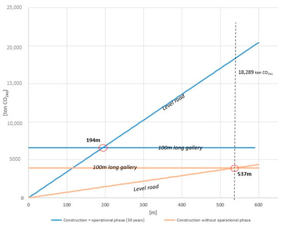
Figure 24.
Comparison between CO2eq emissions of an at-grade road and a tunnel with and without an operational phase.
Another interesting aspect comes from the comparison between traditional concrete (Portland) with more environmentally sustainable types of it, such as those made with eco-cement. In this case, the conversion factor for concrete can be reduced by 50% (following information derived from producers), greatly reducing the impact associated with the use of traditional concrete. Figure 25 shows the results of the impacts relating the construction of the tunnel and the different types of viaducts (low, medium, high), considering the use of green concrete and low-impact steel obtained by recycling using an electric furnace (conversion factor of 0.5 kgCO2/kg of steel [34]). The analysis was limited to road types for which concrete was mostly used. Considering a conversion factor of 50% for conventional concrete, the results show that the use of both sustainable materials reduces the impact by approximately 70% for all sections considered.
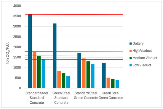
Figure 25.
Comparison of carbon dioxide emissions (ton CO2/F.U.) for the construction of tunnels and viaducts (low, medium, high) using green concrete and green steel.
4.2. Use of Alternative Materials
As part of the environmental impact assessment, with the aim of minimizing negative effects on the environment and local area in the short and long term, this study conducted an in-depth analysis of alternatives aimed at reducing pollutant emissions during the construction phases. Four different alternative solutions were analyzed in comparison with the Alternative 0 proposed in the following study:
- (1)
- Alternative 1 involves the partial replacement of traditional aggregates with recycled materials, specifically replacement of 10% of fine aggregates with recycled glass, both in the wearing course and in the base; replacement of 10% of fine aggregates with heavy ash from incineration, both in the wearing course and in the base; and replacement of 25% of the asphalt in the wearing course and binder course with recycled asphalt;
- (2)
- Alternative 2 considers heavy ashes from the incineration of solid urban waste;
- (3)
- Alternative 3 consists of polymer-modified bitumen;
- (4)
- Alternative 4 consists of recycled concrete.
The analysis focused on emissions of carbon dioxide (CO2), sulfur dioxide (SO2), and nitrogen oxides (NOX) during the construction phase.
The comparison, as shown below, highlighted a modest reduction in emissions during the construction phase for Alternative 1 compared to Alternative 0: reduction in CO2 emissions of approximately 2%; reduction in SO2 emissions of approximately 6%; and reduction in NOX emissions of approximately 9%. With reference to the raw material extraction and production phase (Phase 1 of the LCA), the emissions produced are shown in Table 20 and the related impact categories in Table 21. The emission factors used to calculate emissions are taken from the study by Huang et al. (2009) [5].
Table 20.
Comparison of pollutants emissions between Alternative 0 and Alternative 1.
Table 21.
Comparison between the impact categories of Alternative 0 and Alternative 1.
The second alternative considers the replacement of coarse-grained aggregates in the road foundation layer with heavy ash derived from the incineration of municipal solid waste (MSW), which represents a promising secondary material for construction applications, yet its practical use is constrained by environmental and regulatory challenges. Potential leaching of heavy metals and soluble salts requires adequate treatments such as weathering, washing, or cement-based stabilization [36]. Moreover, the lack of harmonized End-of-Waste criteria limits its large-scale reuse [37]. Despite lower mechanical performance compared to natural aggregates, treated bottom ash can be safely employed in non-structural applications, offering clear benefits in terms of resource efficiency and circularity [38]. The comparative analysis focused on carbon dioxide (CO2), sulfur dioxide (SO2), and nitrogen oxide (NOX) emissions during the construction phase.
The results show a significant percentage reduction in emissions in Alternative 2 compared to Case Study 0:
- –
- CO2: reduction of approximately 56%.
- –
- SO2: reduction of approximately 55%.
- –
- NOX: reduction of approximately 57%.
With reference to the extraction and production phase of raw materials (Phase 1 of the LCA), the emissions generated are shown in Table 22 using emission factors from the study by Olsson et al. (2006) [39] and the environmental impact categories were quantified as reported in Table 23.
Table 22.
Comparison of pollutants emissions between Alternative 0 and Alternative 2.
Table 23.
Comparison between the impact categories of Alternative 0 and Alternative 2.
Alternative 3, based on the use of alternative construction materials, involves replacing 4% of the bituminous conglomerate in the wearing course with a polymer-modified bitumen, specifically styrene–butadiene–styrene (SBS) rubber. This configuration was compared, in terms of pollutant emissions, with road paving made with conventional materials (Alternative 0). The pollutants analyzed were carbon dioxide (CO2), sulfur dioxide (SO2), and nitrogen oxides (NOX).
The comparison showed a quantitatively limited improvement, expressed in percentage terms, in emissions associated with the construction phases. In detail:
- –
- CO2 emissions in Alternative 3 were approximately 4% lower.
- –
- SO2 emissions in Alternative 3 were approximately 5% lower.
- –
- NOX emissions in Alternative 3 are approximately 5% lower.
In summary, considering the extraction and production phases of raw materials (Phase 1 of the Life Cycle Assessment—LCA) related to the construction of road paving, the emissions comparisons between Alternative 0 and Alternative 3 are shown in Table 24, while the environmental impact categories associated with these emissions are shown in Table 25. The emission factors used to calculate emissions are taken from the study by Araújo et al. (2014) [13].
Table 24.
Comparison of pollutants emissions between Alternative 0 and Alternative 3.
Table 25.
Comparison between the impact categories of Alternative 0 and Alternative 3.
Regarding Alternative 4, the results show a significant increase in CO2 and SO2 emissions in Alternative 4, while there is a reduction in NOX emissions. Specifically:
- –
- CO2: approximately 140% increase in Alternative 4;
- –
- SO2: approximately 70% increase in Alternative 4;
- –
- NOX: approximately 90% reduction in Alternative 4.
The increase in CO2 and SO2 emissions is attributable to the higher energy requirements for the primary crushing process of recycled cement. The results of emissions are reported in Table 26 for which the emission factors from the study by Chowdhury et al. (2010) were used [4].
Table 26.
Comparison of pollutants emissions between Alternative 0 and Alternative 4.
Considering the extraction and production phase of raw materials (Phase 1 of the LCA), the resulting environmental impact categories are reported in Table 27.
Table 27.
Comparison between the impact categories of Alternative 0 and Alternative 4.
Analysis of the results obtained shows that all the alternatives examined involve a reduction in SO2 emissions, CO2 follow the same trend, except for Alternative 4 (use of recycled cement). The latter, in fact, results in an increase in CO2 emissions of approximately 2.5 times and SO2 emissions of more than 1.5 times compared to the traditional solution. On the other hand, NOX emissions are reduced by approximately 50%. Alternative 2 (use of heavy ash from the incineration of solid urban waste) is the most advantageous solution, as it allows for a reduction of approximately 50% in the emissions of the pollutants considered in terms of ton and consequently same reduction in all environmental impact categories. Figure 26, Figure 27 and Figure 28 show the results of the comparative analysis between the alternative materials for road paving, considering the three impact categories of GWP, AP, and EP.
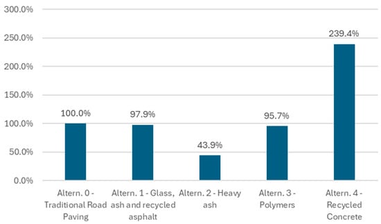
Figure 26.
Comparison between % of CO2eq in the four alternatives scenarios and the case study (Alternative 0, equal to 100%).
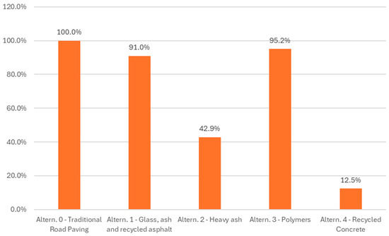
Figure 27.
Comparison between % of SO2eq in the four alternatives scenarios and the case study (Alternative 0, equal to 100%).
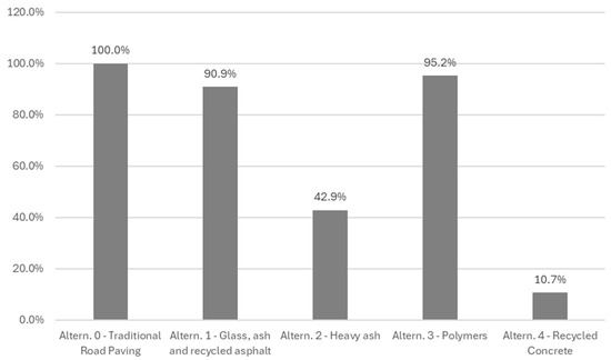
Figure 28.
Comparison between % of PO4eq in the four alternatives scenarios and the case study (Alternative 0, equal to 100%).
In conclusion, based on the data presented, Alternative 2 can be considered the optimal solution for road paving, subject to further considerations not included in this study. However, the choice of the most suitable alternative may vary depending on specific environmental objectives. For example, Alternative 4, while involving a worsening of the GWP as a result of the greater energy consumption for crushing the material, results in a significant improvement in terms of the Acidification Potential of soils and water (AP) and the eutrophication of water bodies (EP).
Since each of the materials mentioned has specific advantages, limitations, and critical issues affecting various areas, the interest should not be focused just on emissions; Table 28 reports a summary of the main aspects relating to the analyzed materials.
Table 28.
Comparison between advantages, limitations, and challenges of alternative materials used.
5. Sensitivity Analysis
The sensitivity analysis was conducted only for the operating phase and for the selected ADT values. This is because ADT is the only, or at least the most significant, parameter whose changes in values can affect the results in terms of impact on the various environmental categories considered. This study conducted the analysis considering an annual percentage increase of 1% starting from a value of 12,550 vehicles/day (ratio between annual traffic volume and measurement days). In the sensitivity analysis, we considered doubling this starting value (obtaining 25,100 vehicles/day) and halving it (equal to 6275 vehicles/day). The extent to which the results were modified in terms of the impact categories shown in Table 29 was therefore examined.
Table 29.
Comparison of results in different environmental impact categories based on ADT equal to the case study value, double that value, and half that value.
6. Conclusions
This study arises from the need to quantify the benefits and potential impacts on the environment and human health associated with the entire life cycle of various types of roadway cross-sections.
This study includes the extraction of raw materials as well as the processing and pro-duction of materials used for the construction of road embankments. Transport for supply and waste disposal was also considered. Finally, the operational phase was considered, assuming a useful life of 30 years for the road sections. The input and output data considered in the analysis are, respectively, consumption of raw materials and energy (thermal or electrical) as inputs, and waste and atmospheric emissions as outputs. Each roadway section consists of the same pavement structure, made from the following raw materials: concrete (for gutters and structural parts of viaducts and tunnels), steel (for guardrails and structural parts of viaducts and tunnels), bituminous mixtures, aggregates, and earth and rock fill for road embankments.
From the results, it emerged that the most significant metric, in terms of environmental and human health impact, was GWP, and the most impactful phases for climate change were material extraction and production (Phase 1) and the operational phase (Phase 4).
The first part of the study compared the emissions associated with the construction (considering the first three phases) of an at-grade road with those of a tunnel, with the latter having a significantly greater impact. The emissions for the realization of 100 m of tunnel can be considered equivalent to those produced by 534 m of road at grade. The conclusion: in the short term (covering only up to Phase 3), a longer at-grade road—up to 537% longer—is environmentally less impactful than a tunnel.
However, including the operational Phase 4, a 537 m at-grade road emits nearly three times (277%) the CO2 of a 100 m tunnel. Therefore, parity of emissions between different lengths is reached only when the at-grade section is approximately 94% the length of the tunnel. This suggests considering that up to that value, the section at ground level could be advantageous from a sustainability point of view, while above that value, the use of a tunnel could be more sustainable.
Finally, as part of evaluating environmental impacts with the goal of minimizing negative effects in the short and long term, a set of alternatives was analyzed to reduce pollutant emissions during the construction phase. Four construction material alternatives were then proposed and assessed; their combination with the defined roadway sections allowed quantification of emission reductions. The results analysis highlighted that all alternatives led to reductions in CO2 and SO2 emissions, except Alternative 4 (use of recycled cement), which resulted in about 2.5-fold higher CO2 emissions as a result of the greater energy consumption for crushing the material and over 1.5-fold higher SO2 emissions compared to the traditional solution. However, NOx ; emissions were reduced by about 50%. Alternative 2 (use of bottom ash from municipal solid waste incineration) emerged as the most advantageous solution, achieving approximately a 50% reduction in all considered pollutants. That said, the optimal choice may vary depending on specific environmental objectives; for instance, Alternative 4, while worsening the GWP, provides significant improvements in Acidification Potential (AP) and Eutrophication Potential (EP). The fact that the use of bottom ash results in a more sustainable approach compared with the recycling of concrete derives from the fact that the production of MSW ash allows for the production of energy not from oil supplies, while the preparation of recycled concrete results in a high energetic procedure.
The LCA model can then be used as a decision-support tool for sustainable construction in the road industry. In fact, the present study offers an integrated methodology model which, already in the road section definition phase, takes environmental impacts into account in a predictive manner.
All considerations presented in the study excluded economic aspects and any factors unrelated to emissions.
7. Limitations and Future Work
Although the proposed approach provides valuable insights into the environmental performance of different roadway typologies and materials, several limitations should be acknowledged.
First, the operational phase was limited to the emissions generated by vehicular traffic over a 30-year period, excluding maintenance operations. While this omission does not substantially alter the comparative results—since maintenance frequencies are similar across the analyzed roadway configurations—it may underestimate the total Global Warming Potential (GWP) by approximately 10–25% based on the comparable literature. Future work will extend the system boundaries to include scheduled maintenance interventions and their specific material and energy requirements.
Second, the study did not include validation or benchmarking against established LCA software tools such as SimaPro or OpenLCA. Following ISO 14040, 14044, and 14064 standards would mainly result in differences in characterization factors and database choices, potentially leading to variations in quantitative results. However, the primary purpose of this research was not to replicate existing commercial software, but rather to demonstrate how the LCA methodology can be implemented within a simplified, transparent, and customizable decision-support framework for infrastructure design.
A separate, dedicated study will therefore focus on a full benchmarking and sensitivity analysis to assess the consistency and robustness of the results against standard LCA tools.
Finally, economic and social dimensions were not considered. A more holistic sustainability assessment should integrate Life Cycle Costing (LCC) and Social LCA (S-LCA) to complement the environmental evaluation, particularly for projects involving public investment and community impacts. Similarly, future developments could incorporate traffic intensity variations, technological evolution in vehicle efficiency, and different climatic conditions, which may significantly influence long-term performance and emissions.
Author Contributions
Conceptualization, P.V. and M.D.P.; methodology, L.C., S.T. and V.V.; software, L.C. and S.T.; validation, P.V., L.C. and F.T.; resources, P.V. and M.D.P.; data curation, L.C. and S.T.; writing—original draft preparation, L.C.; writing—review and editing, L.C. and S.T.; supervision, P.V. All authors have read and agreed to the published version of the manuscript.
Funding
This research received no external funding.
Institutional Review Board Statement
Not applicable.
Informed Consent Statement
Not applicable.
Data Availability Statement
The data presented in this study are available on request from the corresponding author.
Conflicts of Interest
The authors declare no conflicts of interest.
Abbreviations
The following abbreviations are used in this manuscript:
| ADT | Average Daily Traffic |
| ADTV | Average Daily Traffic Volumes |
| ANAS | National Autonomous Road Authority |
| AP | Acidification Potential |
| BC | Bituminous Conglomerate |
| BEVs | Diesel and Electric Vehicles |
| C&D | Construction and Demolition |
| CM | Cement Mix |
| CML-IA | Centrum voor Milieukunde, Leiden |
| EP | Eutrophication Potential |
| F.U. | Functional Unit |
| GM | Granular Mix |
| GWP | Global Warming Potential |
| H | Hierarchist |
| HTP | Human Toxicity Potential |
| IBA | Incinerator Bottom Ash |
| IPCC | Intergovernmental Panel on Climate Change |
| ISO | International Organization for Standardization |
| LCA | Life Cycle Assessment |
| LCI | Life Cycle Inventory |
| LCIA | Life Cycle Impact Assessment |
| MSW | Municipal Solid Waste |
| PNIEC | Integrated National Energy and Climate Plan |
| POCP | Photochemical Ozone Creation Potential |
| RAP | Recycled Asphalt Pavement |
| SBS | Styrene-Butadiene-Styrene |
References
- ISO 14040:2006; Environmental Management-Life Cycle Assessment-Principles and Framework. ISO: Geneva, Switzerland, 2006.
- ISO 14044:2006; Environmental Management-Life Cycle Assessment-Requirements and Guidelines Management Environnemental-Analyse Du Cycle de Vie-Exigences et Lignes Directrices. ISO: Geneva, Switzerland, 2006.
- Birgisdóttir, H.; Bhander, G.; Hauschild, M.Z.; Christensen, T.H. Life Cycle Assessment of Disposal of Residues from Municipal Solid Waste Incineration: Recycling of Bottom Ash in Road Construction or Landfilling in Denmark Evaluated in the ROAD-RES Model. Waste Manag. 2007, 27, 75–84. [Google Scholar] [CrossRef]
- Chowdhury, R.; Apul, D.; Fry, T. A Life Cycle Based Environmental Impacts Assessment of Construction Materials Used in Road Construction. Resour. Conserv. Recycl. 2010, 54, 250–255. [Google Scholar] [CrossRef]
- Huang, Y.; Bird, R.; Heidrich, O. Development of a Life Cycle Assessment Tool for Construction and Maintenance of Asphalt Pavements. J. Clean. Prod. 2009, 17, 283–296. [Google Scholar] [CrossRef]
- Moretti, L.; Mandrone, V.; D’Andrea, A.; Caro, S. Evaluation of the Environmental and Human Health Impact of Road Construction Activities. J. Clean. Prod. 2018, 172, 1004–1013. [Google Scholar] [CrossRef]
- Navon, R.; Shpatnitsky, Y. A Model for Automated Monitoring of Road Construction. Constr. Manag. Econ. 2005, 23, 941–951. [Google Scholar] [CrossRef]
- Tavakoli Mehrjardi, G.; Azizi, A.; Haji-Azizi, A.; Asdollafardi, G. Evaluating and Improving the Construction and Demolition Waste Technical Properties to Use in Road Construction. Transp. Geotech. 2020, 23, 100349. [Google Scholar] [CrossRef]
- Zhou, Y.; Tong, C.; Wang, Y. Road Construction, Economic Growth, and Poverty Alleviation in China. Growth Change 2022, 53, 1306–1332. [Google Scholar] [CrossRef]
- Xu, S.; Sun, C.; Wei, H.; Hou, X. Road Construction and Air Pollution: Analysis of Road Area Ratio in China. Appl. Energy 2023, 351, 121794. [Google Scholar] [CrossRef]
- Segui, P.; Safhi, A.e.M.; Amrani, M.; Benzaazoua, M. Mining Wastes as Road Construction Material: A Review. Minerals 2023, 13, 90. [Google Scholar] [CrossRef]
- Mäki, S.; Kalliola, R.; Vuorinen, K. Road Construction in the Peruvian Amazon: Process, Causes and Consequences. Environ. Conserv. 2001, 28, 199–214. [Google Scholar] [CrossRef]
- Araújo, J.P.C.; Oliveira, J.R.M.; Silva, H.M.R.D. The Importance of the Use Phase on the LCA of Environmentally Friendly Solutions for Asphalt Road Pavements. Transp. Res. Part D Transp. Environ. 2014, 32, 97–110. [Google Scholar] [CrossRef]
- Hausberger, L.; Flora, M.; Gschösser, F. Environmental Impacts of Road Traffic and Route Variants: An Accurate Way to Support Decision-Making Processes of Mountain Roads and Tunnels in Austria. Buildings 2025, 15, 1669. [Google Scholar] [CrossRef]
- Aryan, Y.; Dikshit, A.K.; Shinde, A.M. Life Cycle Environmental Assessment of State and National Highways in India: Evaluating Impact Reduction Potential of Sustainable Measures. Environ. Impact Assess. Rev. 2025, 114, 107944. [Google Scholar] [CrossRef]
- Batuecas, E.; Tommasi, T.; Battista, F.; Negro, V.; Sonetti, G.; Viotti, P.; Fino, D.; Mancini, G. Life Cycle Assessment of Waste Disposal from Olive Oil Production: Anaerobic Digestion and Conventional Disposal on Soil. J. Environ. Manag. 2019, 237, 94–102. [Google Scholar] [CrossRef]
- Sappa, G.; Iacurto, S.; Ponzi, A.; Tatti, F.; Torretta, V.; Viotti, P. The LCA Methodology for Ceramic Tiles Production by Addition of MSWI BA. Resources 2019, 8, 93. [Google Scholar] [CrossRef]
- Viotti, P.; Tatti, F.; Bongirolami, S.; Romano, R.; Mancini, G.; Serini, F.; Azizi, M.; Croce, L.; Pubblica Sabina Sp, A. Life Cycle Assessment Methodology Applied to a Wastewater Treatment Plant. Water 2024, 16, 1177. [Google Scholar] [CrossRef]
- Trunzo, G.; Moretti, L.; D’Andrea, A. Life Cycle Analysis of Road Construction and Use. Sustainability 2019, 11, 377. [Google Scholar] [CrossRef]
- Mroueh, U.; Eskola, P.; Laine-ylijoki, J.; Juvankoski, E.M.M.; Wellman, K.; Ruotoistenmäki, A. Life Cycle Assessment of Road Construction-Finnra Reports 17/2000; Finnish National Road Administration Finnra: Helsinki, Finland, 2000; ISBN 9517266332. [Google Scholar]
- Jullien, A.; Dauvergne, M.; Cerezo, V. Environmental Assessment of Road Construction and Maintenance Policies Using LCA. Transp. Res. Part D Transp. Environ. 2014, 29, 56–65. [Google Scholar] [CrossRef]
- Abedin Khan, Z.; Balunaini, U.; Costa, S. Environmental Feasibility and Implications in Using Recycled Construction and Demolition Waste Aggregates in Road Construction Based on Leaching and Life Cycle Assessment–A State-of-the-Art Review. Clean. Mater. 2024, 12, 100239. [Google Scholar] [CrossRef]
- Tillman, A.M. Significance of Decision-Making for LCA Methodology. Environ. Impact Assess. Rev. 2000, 20, 113–123. [Google Scholar] [CrossRef]
- Schrijvers, D.L.; Loubet, P.; Sonnemann, G. Developing a Systematic Framework for Consistent Allocation in LCA. Int. J. Life Cycle Assess. 2016, 21, 976–993. [Google Scholar] [CrossRef]
- Bjørn, A.; Diamond, M.; Owsianiak, M.; Verzat, B.; Hauschild, M.Z. Strengthening the Link between Life Cycle Assessment and Indicators for Absolute Sustainability to Support Development within Planetary Boundaries. Environ. Sci. Technol. 2015, 49, 6370–6371. [Google Scholar] [CrossRef]
- Hou, Q.; Mao, G.; Zhao, L.; Du, H.; Zuo, J. Mapping the Scientific Research on Life Cycle Assessment: A Bibliometric Analysis. Int. J. Life Cycle Assess. 2015, 20, 541–555. [Google Scholar] [CrossRef]
- Chen, H.; Yang, Y.; Yang, Y.; Jiang, W.; Zhou, J. A Bibliometric Investigation of Life Cycle Assessment Research in the Web of Science Databases. Int. J. Life Cycle Assess. 2014, 19, 1674–1685. [Google Scholar] [CrossRef]
- Balaguera, A.; Carvajal, G.I.; Albertí, J.; Fullana-i-Palmer, P. Life Cycle Assessment of Road Construction Alternative Materials: A Literature Review. Resour. Conserv. Recycl. 2018, 132, 37–48. [Google Scholar] [CrossRef]
- Kucukvar, M.; Tatari, O. Ecologically Based Hybrid Life Cycle Analysis of Continuously Reinforced Concrete and Hot-Mix Asphalt Pavements. Transp. Res. Part D Transp. Environ. 2012, 17, 86–90. [Google Scholar] [CrossRef]
- Yu, B.; Lu, Q.; Xu, J. An Improved Pavement Maintenance Optimization Methodology: Integrating LCA and LCCA. Transp. Res. Part A Policy Pract. 2013, 55, 1–11. [Google Scholar] [CrossRef]
- Celauro, C.; Corriere, F.; Guerrieri, M.; Lo Casto, B. Environmentally Appraising Different Pavement and Construction Scenarios: A Comparative Analysis for a Typical Local Road. Transp. Res. Part D Transp. Environ. 2015, 34, 41–51. [Google Scholar] [CrossRef]
- Ferreira, V.J.; Sáez-De-Guinoa Vilaplana, A.; García-Armingol, T.; Aranda-Usón, A.; Lausín-González, C.; López-Sabirón, A.M.; Ferreira, G. Evaluation of the Steel Slag Incorporation as Coarse Aggregate for Road Construction: Technical Requirements and Environmental Impact Assessment. J. Clean. Prod. 2016, 130, 175–186. [Google Scholar] [CrossRef]
- Ekvall, T.; Weidema, B.P. System Boundaries and Input Data in Consequential Life Cycle Inventory Analysis. Int. J. Life Cycle Assess. 2004, 9, 161–171. [Google Scholar] [CrossRef]
- Blanco Perez, S.; Arcipowska, A.; Fiorese, G.; Maury, T.; Napolano, L. Defining Low-Carbon Emissions Steel: A Comparative Analysis of International Initiatives and Standards; JRC Publications: Brussels, Belgium, 2025; ISBN 978-92-68-26730-1. [Google Scholar]
- Caputo, A. Efficiency and Decarbonisation Indicators of the National Energy System and the Electricity Sector; Italian Institute for Environmental Protection and Research: Rome, Italy, 2022; ISBN 978-88-448-1107-5. (In Italian)
- Grosso, M.; Biganzoli, L.; Rigamonti, L. A Quantitative Estimate of Potential Aluminium Recovery from Incineration Bottom Ashes. Resour. Conserv. Recycl. 2011, 55, 1178–1184. [Google Scholar] [CrossRef]
- Istituto Superiore per la Protezione e Ricerca Ambientale. 380/2022 Rapportorifiutiurbani_Ed-2022_N-380_Agg-23_12_2022; Istituto Superiore per la Protezione e la Ricerca Ambientale: Rome, Italy, 2022; ISBN 9788844811457.
- Zhang, T.; Zhao, Z. Optimal Use of MSWI Bottom Ash in Concrete. Int. J. Concr. Struct. Mater. 2014, 8, 173–182. [Google Scholar] [CrossRef]
- Olsson, S.; Kärrman, E.; Gustafsson, J.P. Environmental Systems Analysis of the Use of Bottom Ash from Incineration of Municipal Waste for Road Construction. Resour. Conserv. Recycl. 2006, 48, 26–40. [Google Scholar] [CrossRef]
Disclaimer/Publisher’s Note: The statements, opinions and data contained in all publications are solely those of the individual author(s) and contributor(s) and not of MDPI and/or the editor(s). MDPI and/or the editor(s) disclaim responsibility for any injury to people or property resulting from any ideas, methods, instructions or products referred to in the content. |
© 2025 by the authors. Licensee MDPI, Basel, Switzerland. This article is an open access article distributed under the terms and conditions of the Creative Commons Attribution (CC BY) license (https://creativecommons.org/licenses/by/4.0/).