An Interpretable Machine Learning-Based Framework for CO₂ Emission Prediction and Optimization: A Case Study of a University Campus

Abstract

Carbon peaking and carbon neutrality targets have become central to global climate governance. Building accurate CO₂ emission prediction models to forecast trends and inform mitigation strategies is crucial for addressing climate change. This work proposes an interpretable, integrated prediction optimization framework grounded in fine-grained categories and emission factors, coupling seasonal, demographic, and temporal effects. A Random Forest (RF) model, interpreted via SHapley Additive exPlanations (SHAP) and correlation analysis, enables attribution of key drivers and prioritization of control strategies. Using comprehensive data from a university campus located in Shandong Province, we conduct detailed carbon accounting and derive actionable emission reduction plans under two distinct scenarios—high-comfort soft control and low-comfort hard control. Results demonstrate strong applicability to campus “large-scale community” settings, enabling differentiated control across building types and seasons. The framework achieves accurate emission predictions with R² of 0.92, identifies energy consumption as the dominant emission source, and realizes 20–30% reduction potential in key building categories during different seasons while maintaining operational viability. This study provides substantial methodological support for regional CO₂ reduction strategies, sustainable development pathways, and the achievement of carbon-neutrality goals.

1. Introduction

The rise in greenhouse gas (GHG) emissions underscores the urgent need for global action to combat climate change. As awareness of the greenhouse effect and its indirect consequences grows, the “carbon peak-carbon neutrality” target for the middle of this century has become the central focus of global climate governance [1,2,3]. Establishing accurate CO₂ emission prediction models to forecast and understand CO₂ emission trends is essential for mitigating climate change and its impacts [4,5,6,7]. Interpretable carbon emission prediction simulations, which guide practical actions, form the foundational basis and methodological cornerstone for transforming macro-level “dual carbon” objectives into actionable engineering and policy measures [8].

Numerous scholars have developed three types of CO₂ emission accounting models. Statistical and econometric models use activity data and emission factors to calculate target sequences and model them over time. These models are primarily employed for medium- and long-term trend forecasting and are suitable for industries where emission relationships are approximately linear. However, they tend to accumulate errors due to data fluctuations under strong non-linearity and cross-scale coupling conditions, which limits their accuracy [9,10]. Spatio-temporal models jointly model both the time and space dimensions, considering time lags and spatial heterogeneity. These models are often used for regional-level spatio-temporal forecasting and CO₂ emission backcasting, enhancing both accuracy and interpretability in systems with spatial dependencies and neighboring interactions. However, their stability and extrapolation capabilities are significantly limited when data is sparse [11]. Probabilistic models use statistical methods to describe the multi-scale characteristics of CO₂ emissions and output interval forecasts, typically applied in short-to-medium-term, seasonally significant, and volatile scenarios [12,13]. In summary, these methods rely on limited data and mostly focus on trend prediction and conclusive judgment. Their coupling with decision optimization remains weak, making it difficult to structurally transmit uncertainty to control and scheduling layers. This limits their ability to support real-time and precise regulation of production and operation within a region.

Compared to traditional models, machine learning offers significant advantages in handling nonlinear, multimodal, and time-varying features, and it can be coupled with interpretability methods to enhance reliability. Existing studies have directly integrated machine learning methods into CO₂ emission prediction. For building or district-based models, machine learning models such as Extreme Gradient Boosting (XGBoost) are commonly used, and Model Predictive Control (MPC) incorporates variables such as electricity prices, carbon intensity, and comfort into constraints for global optimization [14,15]. Various improvement frameworks, such as opportunity constraints and Distributionally Robust Optimization (DRO), are used to predict and make decisions on CO₂ emissions under uncertainty, ensuring the reliability of strategies [16,17,18,19,20]. Additionally, some studies have coupled carbon-aware demand response by integrating real-time or day-ahead carbon intensity signals into scheduling, often paired with deep learning methods to jointly predict and optimize carbon benefit structures [21,22]. For CO₂ emission optimization, multi-objective optimization is often employed to balance CO₂ emissions, economic costs, and comfort, using tree models to search the Pareto front for compromise solutions [23,24,25]. Machine learning encompasses all aspects of CO₂ emission prediction methods and can provide valuable guidance. These models can achieve high precision, resilience to fluctuations, and uncertainty description under large-scale data conditions. Furthermore, they play a crucial role in regional scheduling optimization, providing real-time strategies and guidance for regional CO₂ emissions.

However, a gap remains in coupling interpretable predictions with actionable optimization across diverse scenarios. Our work bridges this by integrating explainable machine learning with scenario-based emission control. In this study, we propose a CO₂ emission modeling framework built on fine-grained categories and emission factors, explicitly accounting for seasonal differences and temporal effects. The model takes the reduction in building energy consumption as the decision variable and is bounded by operational and population constraints. Using an RF algorithm combined with SHAP and correlation matrices, it enables interpretable emission prediction and strategy formulation. An empirical study on the campus shows that the framework is well-suited to “micro-city” settings: it accurately accounts for CO₂ emissions across different scenarios, clearly disentangles the impacts of seasonal, demographic, and environmental factors, and, on this basis, delivers scenario-specific optimal solutions—findings that are of significant relevance to sustainable development and achieving carbon neutrality targets.

2. Method

2.1. Carbon Emission Calculation

We proposed a regional carbon emission calculation method that encompasses multiple factors, including electricity consumption, transportation, population activities, and others.

The carbon emissions from energy consumption are defined as the sum of the product of the energy consumption in each sector and the corresponding carbon emission factor. The carbon emissions from energy consumption ${CO}_2^{energy}$ are represented by Equation (1) as follows:

$${CO}_2^{energy}=\sum _{i=1}^a{E}_i\times {EF}_i$$

(1)

where $E_i$ represents the energy consumption in the $i$ category of energy-consuming areas, ${EF}_i$ is the corresponding energy emission factor, and $a$ is the total number of categories. The carbon emissions from transportation work ${CO}_2^{trans}$ can be calculated using Equation (2) as follows:

$${CO}_2^{trans}=\sum _{j=1}^b\left(N_j\times F_j\times D_j\times {EF}_j\times a_j\right)$$

(2)

where $N_j$ represents the number of vehicles of the $j$ category, $F_j$ is the energy consumption per kilometer, $D_j$ is the distance per day, ${EF}_j$ is the carbon emission factor for the $j$ category of vehicles, $a_j$ is the utilization rate of the vehicle, $b$ is the total number of categories in transportation.

The CO₂ emissions from population activities primarily include food consumption. The carbon emissions from population activities ${CO}_2^{food}$ can be calculated using Equation (3) as follows:

$${CO}_2^{food}=P\times \left(F_{meat}\times {EF}_{meat}+F_{veg}\times {EF}_{veg}\right)/\eta$$

(3)

where $P$ is the total population of the region, $F_{meat}$ and $F_{veg}$ represent the per capita consumption of meat and vegetables, respectively, and ${EF}_{meat}$ and ${EF}_{veg}$ are the carbon emission factors for meat and vegetables, respectively. $\eta$ represents the proportion of food that is not wasted. The carbon emissions ${CO}_2^{ind}$ from industrial production can be calculated using Equation (4) as follows:

$${CO}_2^{ind}=\sum _{l=1}^q{E}_l\times {EF}_l$$

(4)

where $E_l$ represents the quantity of the $l$-th type of industrial products produced or purchased, and ${EF}_l$ is the carbon emission factor per unit of production capacity for the $l$-th industrial product, and $q$ is the total number of industrial product categories [26]. Forests and green spaces play a significant role in carbon sequestration. The effects of forest spaces ${CO}_2^{forest}$ and green spaces ${CO}_2^{green}$ on carbon emissions are quantified using Equations (5) and (6).

$${CO}_2^{forest}=A_{forest}\times C_{forest}$$

(5)

$${CO}_2^{green}=A_{green}\times C_{green}$$

(6)

where $A_{forest}$ and $A_{green}$ represent the areas of forest and green spaces, respectively, and $C_{forest}$ and $C_{green}$ represent the carbon sequestration per unit area per day for forests and green spaces, respectively.

In addition to the aforementioned primary factors, regional carbon emissions are also influenced by other factors, such as waste management and industrial emissions. The carbon emissions ${CO}_2^{waste}$ can be estimated using Equation (7) as follows:

$${CO}_2^{waste}=\sum _{k=1}^r\left(W_k\times {EF}_k\right)$$

(7)

where $W_k$ represents the quantity of the $k$-th type of waste or industrial residue, ${EF}_k$ is the carbon emission factor associated with the waste management or industrial residue treatment, and $r$ is the total number of categories in waste treatment.

$$E(t+dt)=f\left(E\right(t),p)$$

(8)

The impact of time lag on CO₂ emissions is determined by Equation (8). For the CO₂ emission ($E\left(t\right)$) at time $t$, after the adjustment by policy $p$ (which includes the lag effect of the policy at that moment), the CO₂ emissions for the next time step or optimized state $E(t+dt)$ can be calculated.

2.2. Statistical Methods and Machine Learning Methods

2.2.1. RF

RF builds multiple independent decision trees by repeatedly sampling the training data and randomly selecting subsets of features for node splitting. During training, each split is determined by minimizing the Gini gain to improve model generalization. In prediction, RF aggregates the votes from all trees to produce the final result, effectively reducing overfitting risk. Tree construction uses the CART algorithm, with pruning applied to control depth and maintain balanced tree structures [27,28,29].

2.2.2. SHAP

After completing model training, we applied a model interpretation tool to analyze and visualize the influence of different features on the prediction results. This study adopted the SHAP method, which is based on the Shapley value theory in game theory, to reasonably allocate the importance of the model output to each input feature, thereby quantifying the contribution of each feature to the prediction. We interpreted the trained RF model to illustrate the distribution of feature importance under low and high feature values, as well as the direction and magnitude of their influence on the output [30,31].

2.2.3. Correlation Matrix

To examine the interrelationships among different building types and emission sources, Pearson correlation coefficient matrices were computed. The correlation coefficient $r_{xy}$ was calculated as Equation (9):

$$r_{xy}={\displaystyle \frac{\sum _{i=1}^s\left(x_i-\bar{x}\right)\left(y_i-\bar{y}\right)}{\sqrt{\sum _{i=1}^s{\left(x_i-\bar{x}\right)}^2}\sqrt{\sum _{i=1}^s{\left(y_i-\bar{y}\right)}^2}}}$$

(9)

where $x_i$ and $y_i$ are observations of two variables, and $\bar{x}$ and $\bar{y}$ are their means. The amount of data of each category involved in the calculation is defined as $s$. The building-level analysis was based on annual CO₂ emissions by building type, while the source-level analysis was based on annual total emissions from each emission source.

2.3. Optimization Method

This study models the optimization as an emissions-minimization problem subject to multiple constraints. Because energy use accounts for the majority of emissions in the region and other factors are difficult to modify, we illustrate the strategy with energy use. Let $x_i\left(m\right)$ denote the relative reduction for building type $i$ in month $m$, and let $E_i\left(m\right)$ be the baseline energy consumption; then the optimized total energy consumption $E^{new}\left(m\right)$ is given by Equation (10).

$$E^{new}\left(m\right)=\sum _{i\in \mathcal{B}}{E}_i\left(m\right)\left[1-x_i\left(m\right)\right]$$

(10)

Using the trained RF model $\widehat{F}$ as the emissions predictor, we minimize the predicted total emissions (Equation (11)) subject to the constraints, where $\mathbf{z}$ denotes the feature vector for CO₂ emissions of each factor. $\lambda$ denotes the strength coefficient of the L1 regularization; $\mathbf{W}\left(m\right)$ is the weight matrix for the building categories; $\mathbf{x}\left(m\right)$ is the vector of reduction ratios for all buildings in month $m$; and $\mathbf{L}\left(m\right)$ is the lower-bound constraint vector.

$$\underset{x\left(m\right)}{min}\widehat{F}[\mathbf{z}\left(m\right),E^{new}\left(m\right)]+\lambda ∥\mathbf{W}\left(m\right)\left(\mathbf{x}\left(m\right)-\mathbf{L}\left(m\right)\right)∥$$

(11)

Building importance weights are obtained by a weighted fusion of their correlations with total emissions and with population. The weight ratio and the size of the candidate building set are dynamically adjusted according to population scale. Correlations among building types are represented by correlation coefficients. The optimized building energy-use profile is then fed into the prediction model to compute the corresponding total emissions, and the candidate scheme with the smallest predicted value with maximum comfort is selected as the optimal solution. The size of the optimization is measured by policies that take into account the time lag effect and is considered to be a function of population, climate conditions, and time.

For building type $b$ in season $m$, the maximum adjustment in energy consumption $Cut\left(b,m\right)$ can be considered as the product of the policy factor $f_{policy}$, seasonal factor $f_{season}$, and comfort factor $f_{comfort}$ (Equation (12)).

$$Cut\left(b,m\right)=f_{policy}\left(b\right)\times f_{season}\left(m\right)\times f_{comfort}\left(b,m\right)$$

(12)

The policy factor is assigned values based on the importance ranking. The seasonal factor is defined as the product of the seasonal adjustment demand $s\left(m\right)$, the vacancy potential of the category $v\left(m\right)$ and the cumulative effect of the obtained time delay $t\left(m\right)$, as described in Equation (13).

$$f_{season}\left(m\right)=s\left(m\right)\times v\left(m\right)\times t\left(m\right)$$

(13)

The comfort coefficient $f_{comfort}\left(b,m\right)$ is defined in Equation (14) as the ratio of the comfort weight $W$ to the product of the temperature effect factor $TE$ and the seasonal comfort adjustment coefficient $CA$. The comfort weight $W$ is determined by the energy reduction requirements of different building types. The temperature effect factor $TE$ is a ratio defined by the difference between the current temperature and 26 °C, divided by the annual maximum temperature range. The seasonal comfort adjustment coefficient $CA$ is itself a ratio, which reflects the relative difficulty and energy cost of maintaining thermal comfort under the given conditions represented by $TE$, compared to the most comfortable scenario.

$$f_{comfort}\left(b,m\right)={\displaystyle \frac{W\left(b\right)}{CA\left(m\right)\times TE\left(b,m\right)}}$$

(14)

3. Results

The university campus located in Shandong Province spans a total area of 1153 acres. Its spatial layout encompasses diverse functional units, including residential zones, teaching and research buildings, public transportation hubs, and experimental R&D parks, collectively forming a relatively enclosed micro-urban ecosystem. This makes it an ideal research sample for analyzing carbon emission characteristics.

We chose to conduct a simulation analysis using data from the years 2023 to 2025, focusing on all elements within the region. For energy utilization, data is collected on an hourly basis, while for population changes, diet, transportation, and other factors, data is collected daily. In this study, we quantify CO₂ emissions on a monthly basis and divide each year into four seasons: spring (March, April, May), summer (June, July, August), autumn (September, October, November), and winter (December, January, February).

3.1. Regional CO₂ Emission Accounting

3.1.1. Analysis of CO₂ Emissions from Energy

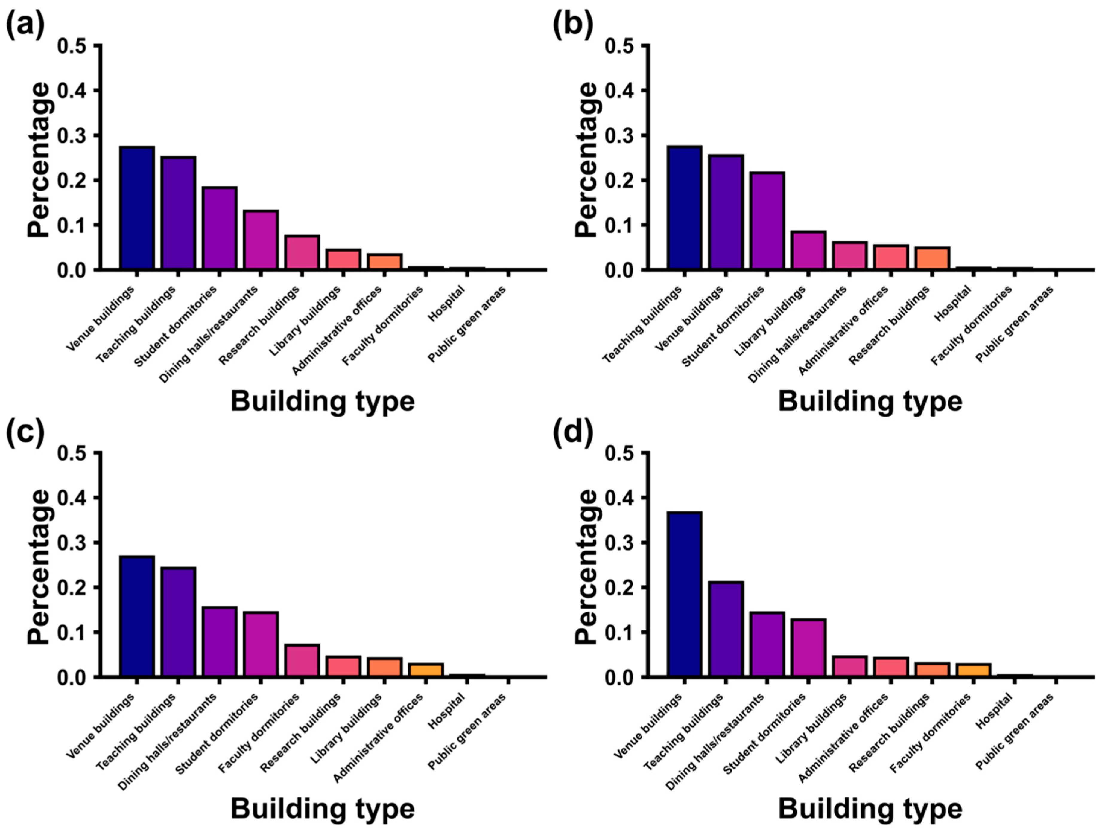
As shown in Figure 1, we have categorized the buildings and architectural accessories into 10 groups: venue buildings, teaching buildings, student dormitories, dining halls/restaurants, research buildings, library buildings, administrative offices, faculty dormitories, hospital, and public green areas. The seasonal energy consumption fluctuations of these ten building categories directly reflect variations in carbon emissions, providing a basis for formulating energy-saving strategies. The energy consumption patterns remain largely consistent during spring and autumn. In summer, the proportion of electricity consumption in student dormitories and teaching buildings increases significantly due to air conditioning usage. In winter, although some students leave campus, the overall energy consumption shows little change due to centralized heating, with venue buildings experiencing a substantial increase in energy demand for heating purposes.

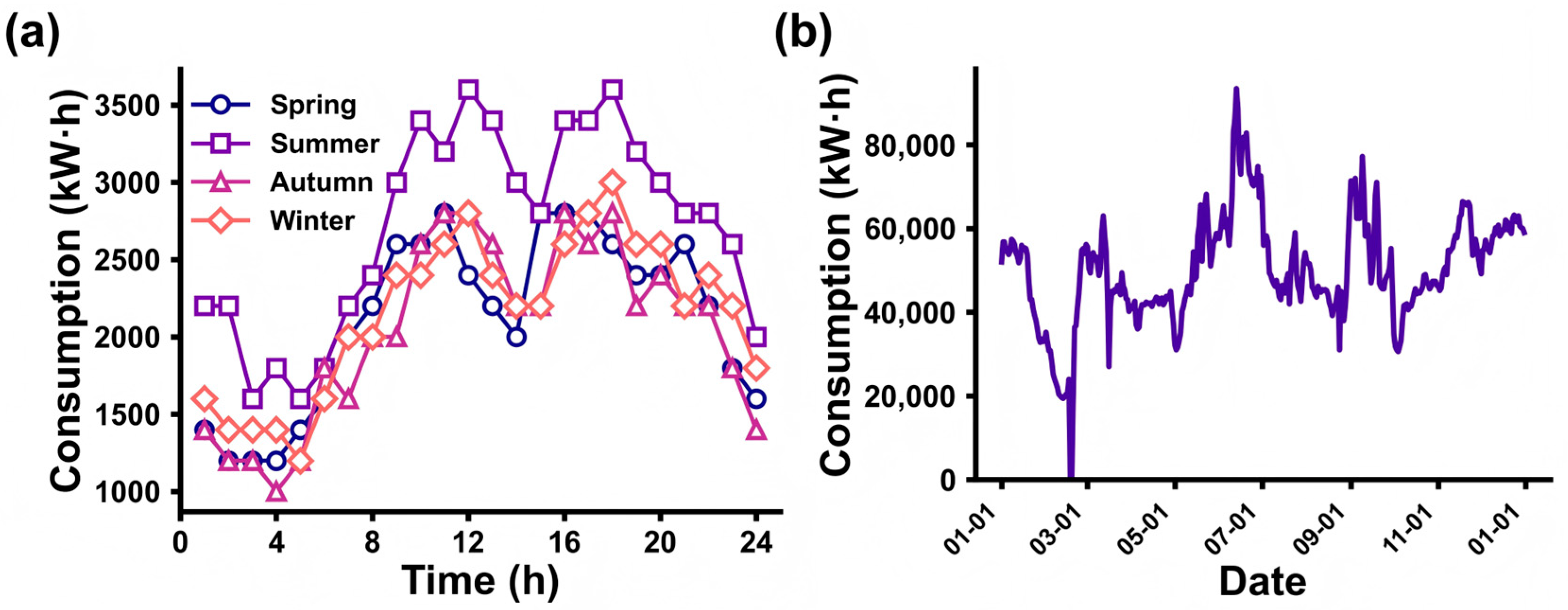
The load fluctuation data serves as a critical parameter for optimizing regional carbon emissions, enabling the formulation of targeted strategies based on temporal characteristics. As illustrated in Figure 2, the overall load profiles demonstrate minimal variations among spring, autumn, and winter seasons for the aforementioned reasons, though winter exhibits slightly higher nighttime loads due to continuous heating demand. In contrast, summer experiences an upward shift in load curves with sustained nighttime consumption, attributable to air conditioning requirements. All seasonal patterns maintain typical peak-valley characteristics in energy supply. Annual energy consumption fluctuations exhibit distinct seasonal patterns, with lower demand in spring/autumn and elevated peaks in winter/summer. Notably, data from the operational suspension during the mid-February Spring Festival period is excluded from modeling. The mid-July to September summer vacation period, characterized by reduced student occupancy and consequent lower energy consumption, provides essential datasets for investigating the impacts of population density and spatial configuration on carbon emissions.

We considered a total of 10 ($i_{max}=10$) types of power consuming facilities in the region. As the studied area exclusively utilizes electricity, a uniform carbon emission factor of 0.6 kg/(kW·h) (

Table 1. Parameter of carbon emissions from energy usage [32].

Parameter	Value
$i_{max}$	10
${EF}_i$	0.6 kg/(kw·h)

) was applied to all building types [32]. In 2024, the total energy consumption reached 18.41 million kW·h, resulting in corresponding CO₂ emissions of 11,004.24 tons. The carbon emissions of each building type at different time intervals exhibit a proportional relationship with either their absolute energy consumption or energy consumption share, and these data will be utilized for subsequent strategy optimization analyses.

3.1.2. Analysis of CO₂ Emissions from Transportation

Table 2. Parameter of carbon emissions from transportation [33,34].

Parameter	Value
$j_{max}$	3
$N_{bicycle}$	792
$N_{elec\text{-}bicycle}$	2836
$N_{car}$	1406
$F_{bicycle}$	0 kW·h/km
$F_{elec\text{-}bicycle}$(4 seasons)	0.012/0.01/0.012/0.025 kW·h/km
$F_{car}$(4 seasons)	0.14/0.17/0.14/0.22 kW·h/km
$D_{bicycle}$(4 seasons)	3.4/2.4/3.6/1.5 km/day
$D_{elec\text{-}bicycle}$(4 seasons)	6.2/7.3/6.4/4.0 km/day
$D_{car}$(4 seasons)	2.5/3.0/2.5/3.8 km/day
${EF}_{bicycle}$	0
${EF}_{elec\text{-}bicycle}$	0.6 kg/(kW·h)
${EF}_{car}$	0.9 kg/(kW·h)
$a_{bicycle}$	0.15
$a_{elec\text{-}bicycle}$	0.5
$a_{car}$	0.2

presents the calculation parameters for transportation carbon emissions, focusing exclusively on three predominant modes of transport: bicycles, electric bicycles, and cars. The analysis assumes a constant inventory of each vehicle type within the study area. In terms of energy consumption per unit distance, bicycles are assigned a zero-value baseline, while the other two categories exhibit distinct seasonal variations—demonstrating comparable consumption patterns during spring and autumn; electric bicycles show reduced energy demand in summer due to eliminated battery preheating requirements at elevated temperatures, whereas cars display increased consumption from air conditioning usage; both vehicle types experience significantly heightened energy demands during winter conditions due to low-temperature effects. The mileage and usage rate data are obtained through regional statistics.

The average daily travel distance varies significantly across transport modes, reflecting users’ climate-dependent mobility preferences. For carbon emission factors: bicycles are considered zero-emission; electric bicycles adopt pure electric mode with an emission factor identical to building electricity use (0.6 kg/(kW·h)); cars use a weighted average of 0.9 kg/(kW·h) based on a 50–50% gasoline-EV mix. Actual vehicle utilization is dynamically scaled according to the real-time population-to-capacity ratio in the area. Due to the small area, the utilization rate of cars is low, only 0.2, while that of electric-bicycles is 0.5.

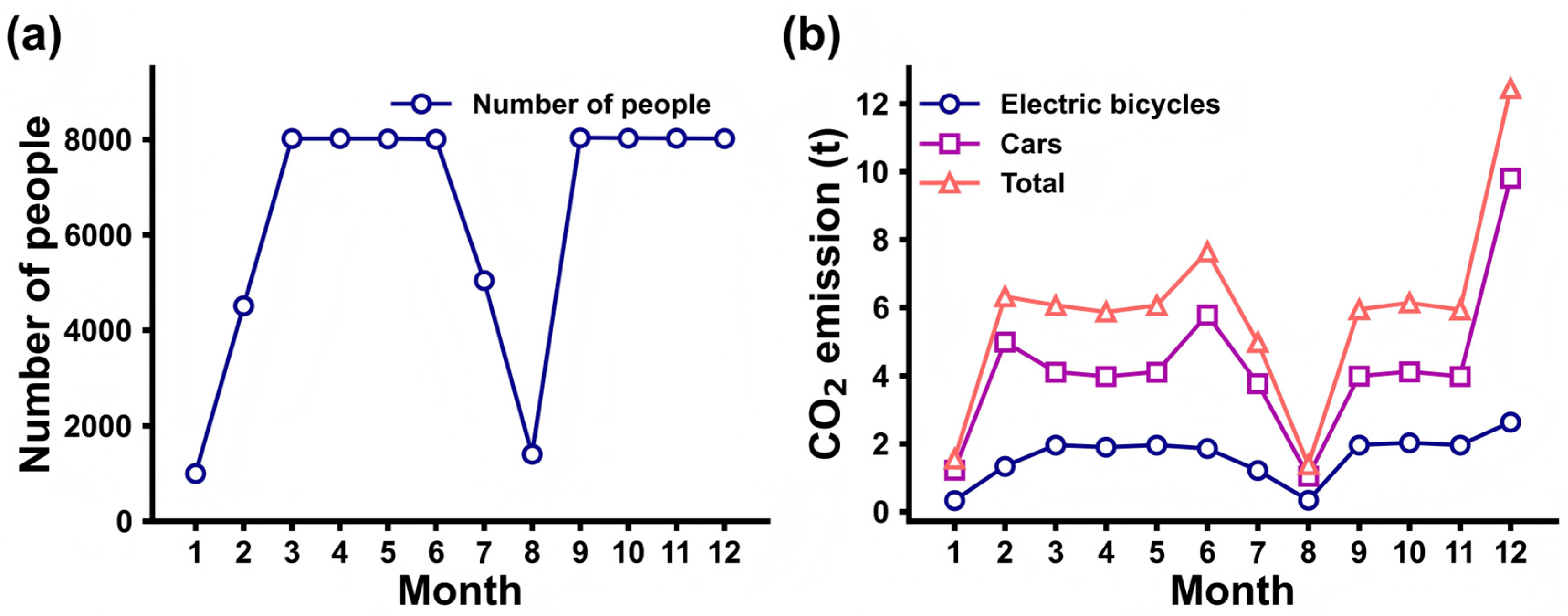
As shown in Figure 3, there are two distinct vacation periods with significantly reduced population within a year, while the population remains relatively stable during the rest of the time. Transportation-related CO₂ emissions exhibit seasonal variations: emissions in spring and autumn hover around the average level with minor fluctuations; summer sees slightly higher per capita emissions, primarily due to increased car usage driven by hot weather, despite the lower energy consumption of electric bicycles being offset by their reduced adoption. In winter, car usage increases further, and although electric bicycles remain little used, their higher energy consumption contributes to additional emissions. Among the four seasons, winter records the highest per capita CO₂ emissions from transportation. The annual transportation-related CO₂ emission in this area is 70.35 tons.

3.1.3. Analysis of CO₂ Emissions from Population Activities

CO₂ emissions from human activities primarily originate from dietary consumption. In this model, the average daily food intake per capita is assumed constant, with meat and vegetable consumption fixed at 0.205 kg/(person·day) and 0.930 kg/(person·day), respectively (

Table 3. Parameter of carbon emissions from population activities [35,36].

Parameter	Value
$F_{meat}$	0.205 kg/(person·d)
${EF}_{meat}$	7.5 kg/kg
$F_{veg}$	0.930 kg/(person·d)
${EF}_{veg}$	0.6 kg/kg
$\eta$	0.85

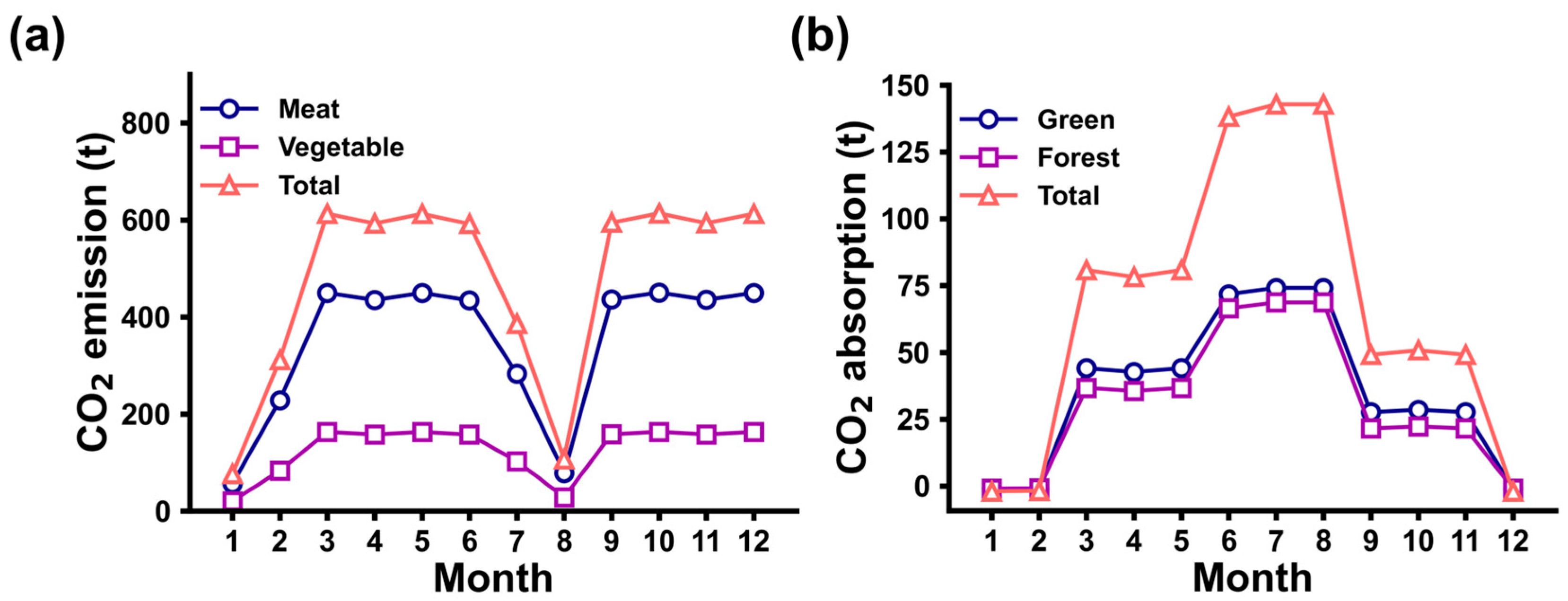
). The carbon emission factors were calculated using dietary habit-weighted averages, yielding mean values of 7.5 kg CO₂/kg for meat and 0.6 kg CO₂/kg for vegetables. The model incorporates a food waste factor, with 85% of food assumed to be actually consumed. As shown in Figure 4a, the monthly variation pattern of these emissions closely follows population fluctuations, with annual CO₂ emissions reaching 5704.57 tons.

3.1.4. Analysis of CO₂ Emissions from Vegetation

The carbon sequestration by vegetation primarily comes from green spaces and forests, covering 167,233 m² and 80,560 m², respectively. Given the study area’s location in North China, the calculation employs region-specific carbon absorption coefficients for typical grasslands and forests (

Table 4. Parameter of carbon sequestrations from vegetation [37].

Parameter	Value
$A_{green}$	167,233 m2
$A_{forest}$	80,560 m2
$C_{green}\left(4\mathrm{s}\mathrm{e}\mathrm{a}\mathrm{s}\mathrm{o}\mathrm{n}\mathrm{s}\right)$	8.5/14.3/5.5/−0.2 g/(m2·d)
$C_{forest}\left(4\mathrm{s}\mathrm{e}\mathrm{a}\mathrm{s}\mathrm{o}\mathrm{n}\mathrm{s}\right)$	14.7/27.5/8.9/−0.4 g/(m2·d)

). Figure 4b shows that vegetation carbon emissions are significantly affected by season, and the annual cumulative carbon emissions are −806.59 tons.

3.1.5. Analysis of CO₂ Emissions from Waste Management

Given the absence of industrial facilities in the study area, industrial emissions have been excluded from the analysis. This research specifically focuses on carbon emissions associated with solid waste and wastewater treatment. The data reveals that monthly solid waste generation fluctuates between 440 and 640 tons per month, with variations driven by factors such as population size and seasonal changes (

Table 5. Parameter of carbon emissions from waste management [38].

Parameter	Value
$m_{max}$	2
$W_{waste}$	440–640 t/month
${EF}_{waste}$	0.5 t/t
$W_{water}$	60.78 t/(person·year)
${EF}_{water}$	0.75 kg/t

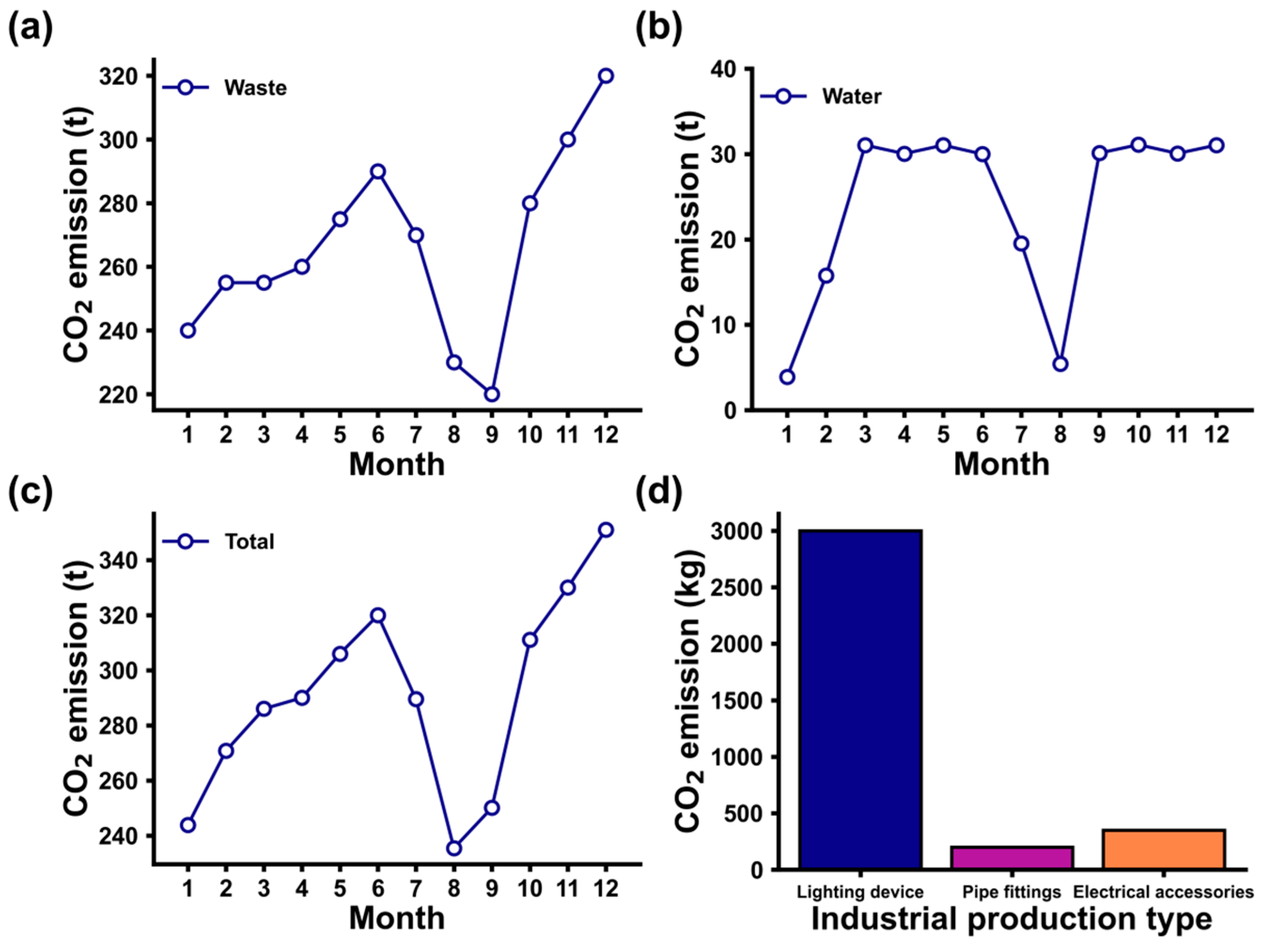
). To estimate emissions, a weighted average of disposal methods (including landfilling and incineration) was applied, resulting in a carbon emission factor for waste treatment of 0.5 kg per ton. As depicted in Figure 5a, monthly CO₂ emissions from solid waste treatment are shown. Notably, the high density of public buildings leads to increased per capita water consumption, which reaches 60.78 tons per person per year. As illustrated in Figure 5b,c, CO₂ emissions from wastewater treatment are closely correlated with regional population size and represent a relatively small proportion of the total CO₂ emissions.

3.1.6. Analysis of CO₂ Emissions from Industrial Production

In the absence of industrial production activities within the study area, industrial-related carbon emissions were limited to facility maintenance processes. This study categorized maintenance emissions into three types: lighting devices, pipe fittings, and electrical accessories, with respective CO₂ emission accounting. As shown in Figure 5d, the CO₂ emissions from facility maintenance were negligible, amounting to only approximately 3.55 tons per year.

3.1.7. Annual CO₂ Emissions Analysis

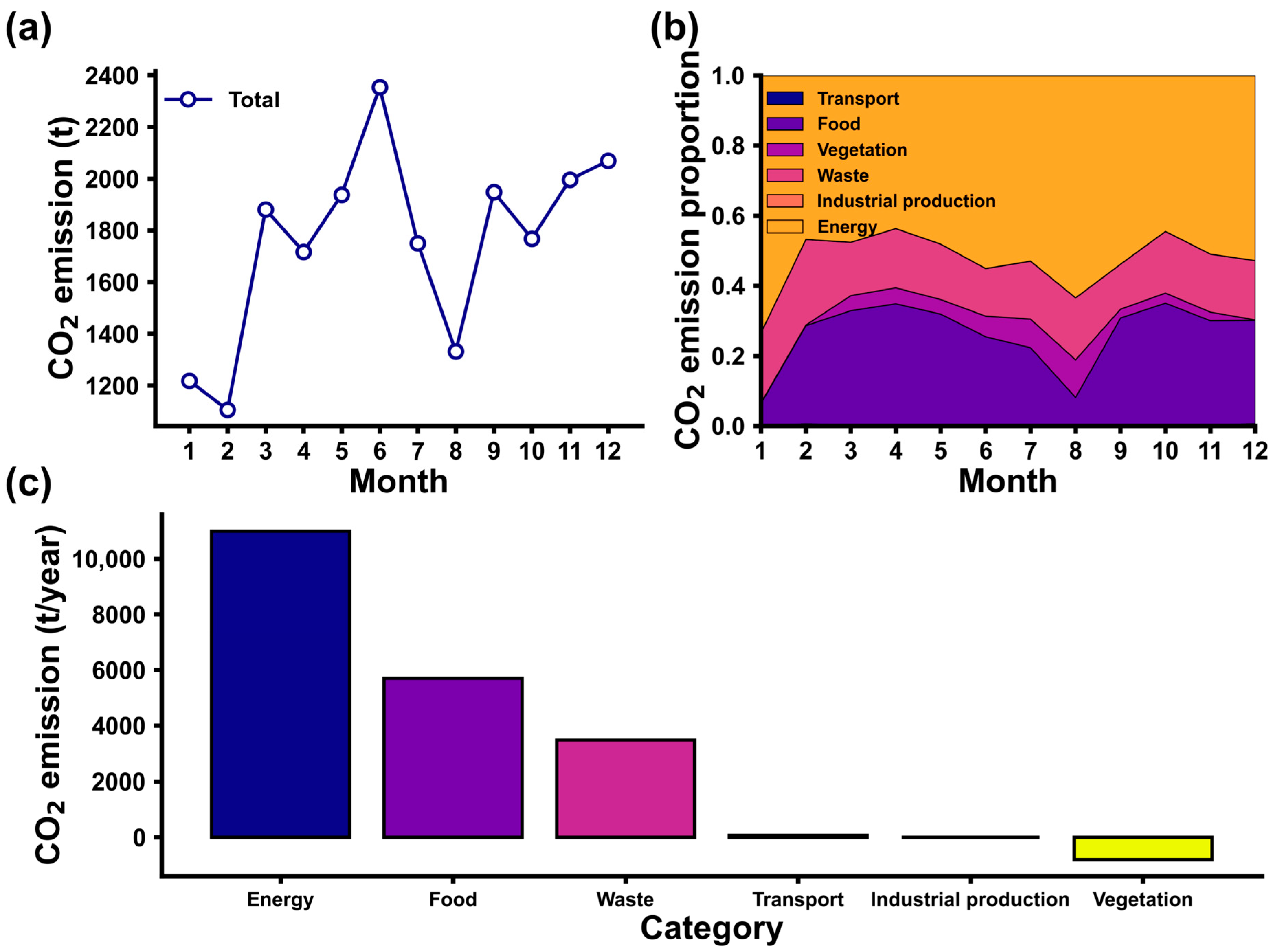
Figure 6a illustrates the annual dynamics of CO₂ emissions in the study area. The emission profile exhibits an “energy-dominant, multi-source synergistic” pattern, where seasonal fluctuations in energy consumption serve as the primary driver of overall emission trends, while contributions from other sources are modulated by demographic mobility and climatic factors. Analytical results reveal that apart from emission troughs during population valleys (February and July–August), monthly emission intensities are predominantly climate-driven, with marked peaks in summer (air conditioning) and winter (space heating). Notably, per capita emissions demonstrate pronounced seasonal variability during high-population periods, whereas during low-population periods, elevated per capita emissions are observed under identical seasonal conditions—a phenomenon attributable to variations in energy efficiency, the mechanistic details of which will be elaborated upon in subsequent sections.

Figure 6b demonstrates that energy consumption maintains its dominant position throughout all months, with monthly emissions (518.6–1295.6 tons) nearly equal to the combined total of the other five categories, underscoring the pivotal role of energy management in regional decarbonization strategies. As the second largest emission source, food consumption highlights the importance of reducing food waste rates for emission mitigation. Waste treatment ranks as the third largest source, showing relatively stable emission patterns due to consistent solid waste generation. Transportation emissions, vegetation carbon sequestration, and industrial maintenance collectively contribute minimally to the regional emission profile. Annual emissions also exhibited a similar trend in Figure 6c, with energy consumption being the largest source at approximately 11,004.24 t.

3.2. Machine Learning and Strategy Optimization

Finally, we constructed a dataset that includes time, season, population size, energy consumption from different buildings, CO₂ emissions from various factors, and total CO₂ emissions. By using total CO₂ emissions as the prediction target, we explored the relationships between emissions and factors such as population and season.

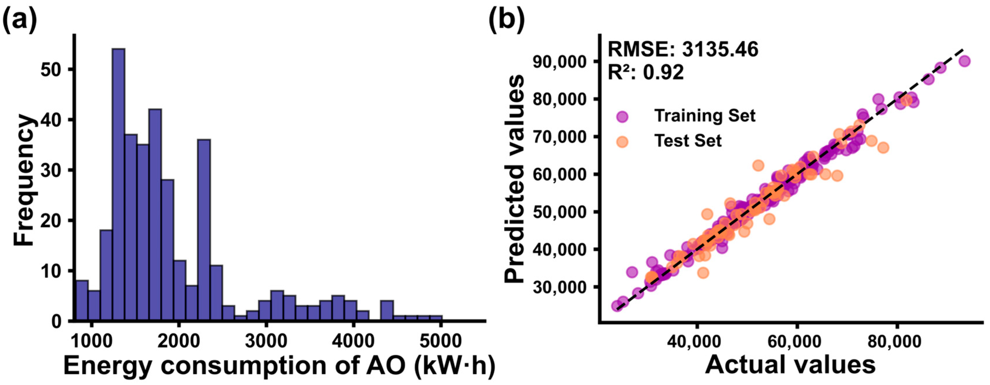
We test the rationality of the data set by the energy consumption distribution of representative administrative offices. Figure 7a shows the energy consumption distribution histogram for administrative offices in the dataset. The data exhibits a skewed distribution, with most of the energy consumption concentrated in the lower range, while higher energy consumption only occurs during specific periods. This demonstrates the reasonableness of the dataset’s size and distribution Based on its superior ability to capture complex data patterns with minimal error and its robust generalization performance that effectively mitigates overfitting, RF was selected as the final model for this study. RF training uses grid search to find the optimal model. Figure 7b displays the results obtained from training the best RF model. The R² value (for the test set) is 0.92, indicating that the model has a good fit. Additionally, the RMSE value is 3135.46, suggesting that the model’s overall performance is quite satisfactory.

4. Discussion

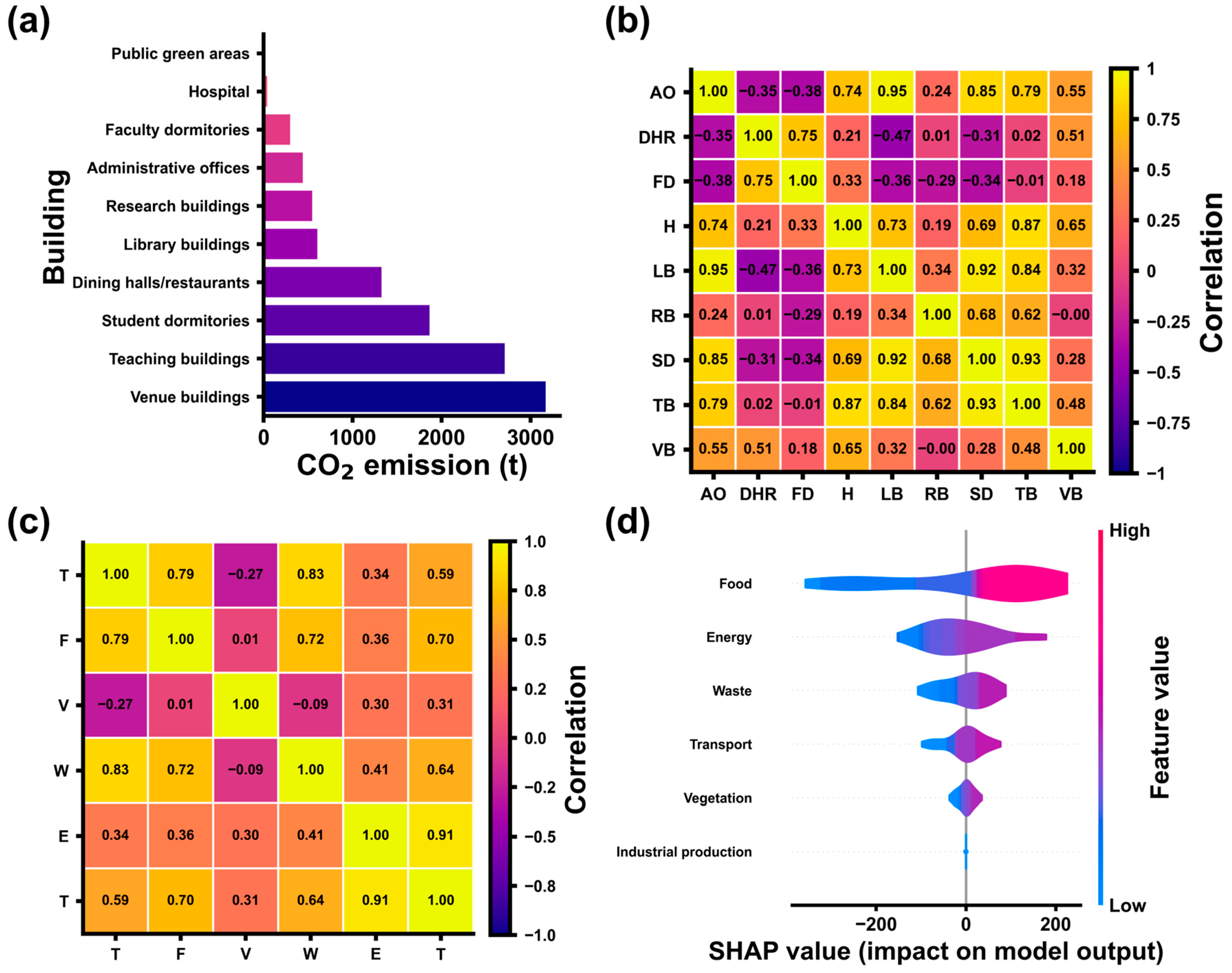
Regarding building-related CO₂ emissions (Figure 8a), the annual CO₂ emissions varied substantially across building types. Venue buildings, teaching buildings, and student dormitories were the major emission sources, each contributing several thousand tons per year, while hospitals, administrative offices, and faculty dormitories had relatively low emissions, and public green areas showed negligible direct emissions. This suggests that emission reduction efforts should prioritize high-consumption building clusters, focusing on retrofitting heating, cooling, lighting, and operational systems for improved efficiency.

Some representative data were selected for correlation coefficient and SHAP analysis. All categories in Figure 8b,c are abbreviated by their first letters. The correlation analysis between building categories (Figure 8b) revealed that most pairs exhibited strong positive correlation coefficients (>0.7), such as administrative offices and library buildings (r = 0.95). This indicates a strong synchronization in energy consumption trends, likely driven by similar climatic conditions and the regional number of occupants. Such synchronization offers opportunities for centralized management and CO₂ emission reduction. The correlation matrix of emission sources (Figure 8c) further revealed that energy consumption had the strongest correlation with total emissions (r = 0.91). Transportation, food, and waste exhibited moderate inter-correlations, while vegetation showed low or negative correlations with other sources, reflecting its carbon sink function and seasonal variations.

The SHAP analysis based on the random forest model (Figure 8d) quantitatively assessed the contributions of each source to total emissions. Food consumption exhibited far greater explanatory power than all other factors, primarily due to population fluctuations and food waste. In the other categories, energy consumption had the largest explanatory power, followed by transport, while waste and vegetation had relatively smaller impacts, and industrial production contributed negligibly. Excluding industrial production, the change in value aligned with the overall trend, and the higher the ranking, the greater the impact of value changes on overall volatility. These findings suggest that emission reduction strategies should prioritize energy efficiency, supported by low-carbon supply chain management in the food sector.

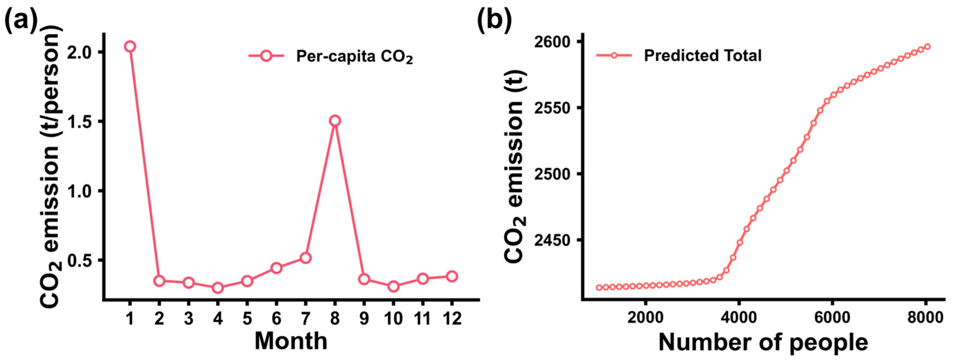
Figure 9a illustrates the monthly variation in per-capita CO₂ emissions, showing a strong correlation with population fluctuations. When the population size is low, per-capita emissions increase markedly. Figure 9b presents the total CO₂ emissions predicted by the RF model across the full population range in July, with a LOWESS-fitted trend curve indicating a monotonically increasing relationship with population density. When the population decreases to a certain threshold, CO₂ emissions gradually level off and stabilize; a similar stabilization is observed when the population approaches its upper limit. These results suggest a correlation between population size and infrastructure energy consumption. At low population levels, the use of public facilities leads to higher per-capita energy consumption; in dormitories, dispersed occupancy and the lack of centralized management reduce the efficiency of air conditioning and other electrical systems. At moderate population levels, the increase in CO₂ emissions per additional person primarily arises from the further opening of public facilities and the increased utilization of dormitories. When the population nears saturation, the energy consumption of public spaces rises only marginally, and concentrated dormitory occupancy enables the sharing of air conditioning and other amenities, thereby slowing the growth rate of CO₂ emissions. Therefore, regional policy changes should be implemented at the inflection point of the curve.

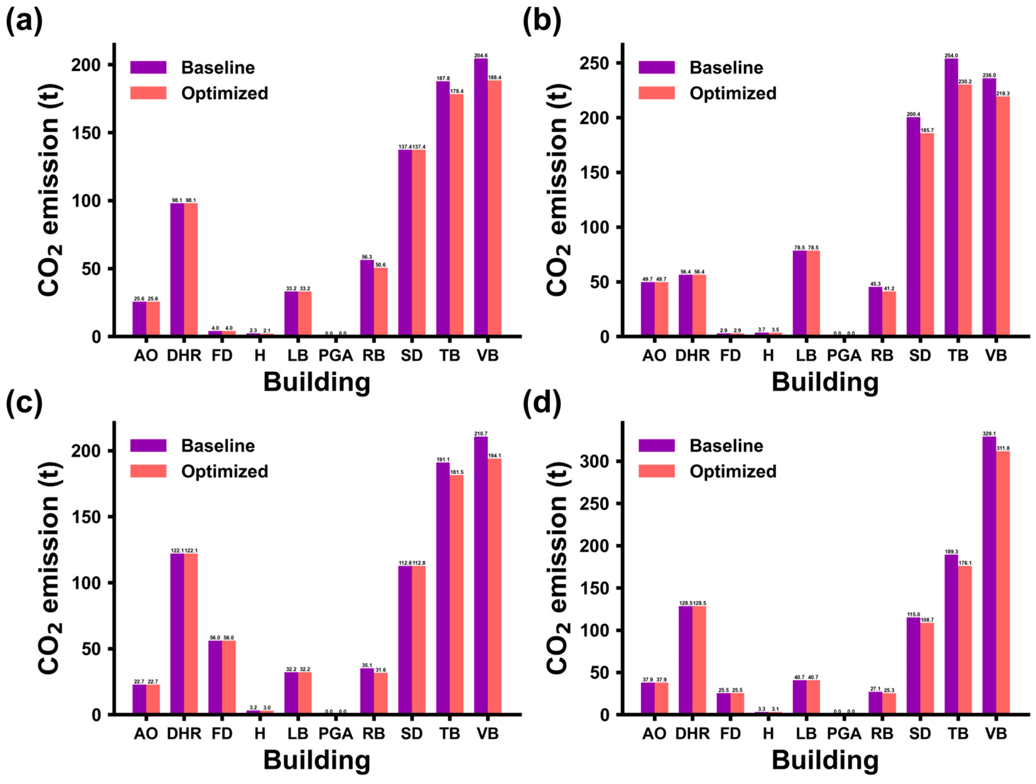
We set up two scenarios for analysis. Scenario 1 involves high comfort with flexible regulation, while Scenario 2 involves low comfort with strict regulation. To compare the differences between the two scenarios, we assume that the seasonal influence factor remains the same in all other aspects and only affects high-population areas such as student dormitories, teaching buildings, and libraries. The seasonal influence is divided into winter–summer and spring–autumn categories. Since accommodation can be centrally managed during off-peak times, the adjustment range is larger, whereas for office buildings, libraries, and similar buildings, which have higher comfort requirements, the maximum adjustment value is considered smaller. For hospitals, due to the highest comfort requirements, the calculated maximum adjustment value is the smallest. The final calculated adjustment range values are shown in

Table 6. Maximum adjustable $Cut\left(b,m\right)$ in scenario 1.

Parameter	$\mathit{C}\mathit{u}\mathit{t}\mathbf{\left(}\mathit{b}\mathbf{,}\mathit{m}\mathbf{\right)}$ Value
Venue buildings	0.2
Teaching buildings	0.1/0.05
Student dormitories	0.2/0
Dining halls/restaurants	0.1
Research buildings	0.1
Library buildings	0.1/0.05
Administrative offices	0.1
Faculty dormitories	0.1
Hospital	0.05

and

Table 7. Maximum adjustable $Cut\left(b,m\right)$ in scenario 2.

Parameter	$\mathit{C}\mathit{u}\mathit{t}\mathbf{\left(}\mathit{b}\mathbf{,}\mathit{m}\mathbf{\right)}$ Value
Venue buildings	0.3
Teaching buildings	0.2/0.1
Student dormitories	0.3/0
Dining halls/restaurants	0.15
Research buildings	0.1
Library buildings	0.2/0.1
Administrative offices	0.2
Faculty dormitories	0.2
Hospital	0.05

. We trained the model on an annual dataset and then optimized it with the mid-month of each quarter, aiming to represent seasonal (quarterly) patterns more faithfully.

Figure 10 compares baseline and optimized CO₂ emissions for major high-consumption building categories after applying the seasonal constraint optimization strategy. The model results indicate that, during summer and winter, reduced dormitory occupancy necessitates centralized management, whereas in spring and autumn—when the population is relatively high—dormitories are not the primary optimization target. In winter and summer, the optimization strategy significantly reduces emissions from student dormitories, teaching buildings, and venue buildings, consistent with their dominant roles in heating and cooling loads. The reason for the smaller decrease in winter compared to summer is that in winter, the entire campus is centrally heated. As a result, centralized management can only reduce electricity and other non-heating consumption. To further decrease CO₂ emissions, it would be necessary to first implement centralized management and then provide targeted heating.

In spring and autumn, the focus of emission reductions shifts toward research buildings, teaching buildings, and venue buildings. However, due to the larger number of people, the emission reductions from these buildings are not as significant overall as during the summer and winter when some areas are closed. Combining building correlation weights with RF-based emission predictions provides an effective and feasible approach for guiding reduction allocation.

In Scenario 2 (Figure 11), the optimization targets minimizing CO₂ emissions, so the model requires all building types to participate in reducing energy use. Taking teaching buildings as an example, although the maximum adjustable rate is 0.1 across seasons, the model still differentiates seasonal effects: in winter, uniform heating makes reductions harder, so the associated strategies are ranked lower and have smaller adjustment magnitudes.

For real-time control, the model can identify existing key peak periods and, along with real-time data on population changes and energy consumption patterns, pre-allocates emission reduction efforts. This enables the formulation of targeted strategies for any given moment. It demonstrates the model’s reliability and its potential for CO₂ emission optimization.

5. Conclusions

We present an interpretable, integrated CO₂ emission prediction–optimization framework grounded in fine-grained categories and emission factors, explicitly accounting for seasonal, demographic, and temporal effects. Using an RF model combined with SHAP and correlation matrices, we enable interpretable prediction and CO₂ strategy design. Using the campus as a representative “large-scale community”, we analyze CO₂ emissions and evaluate optimization strategies under two control scenarios; the model remains robust across conditions. The framework provides a quantitative basis for structurally propagating predictive uncertainty into real-time optimization. The main findings are as follows:

• We develop an interpretable prediction–optimization framework for CO₂ emissions and introduce ML-based optimization schemes that support differentiated control and optimization across building types and seasonal contexts. By integrating RF with SHAP analysis, our framework achieves an R² of 0.92 and identifies key drivers, enabling tailored emission strategies that balance reduction targets with operational comfort constraints.
• We integrate hourly/daily/monthly/quarterly data within a unified model, enabling CO₂ prediction and optimization across multiple temporal scales. This multi-scale data integration captures both short-term fluctuations and long-term seasonal trends, ensuring that predictive accuracy and optimization strategies are robust and adaptable to dynamic changes in population activity and climate conditions.
• We complete carbon accounting for the campus, reveal the characteristic CO₂ emission patterns of a typical micro-city, quantify factor contributions, and provide actionable optimization directions for similar regions. In this campus case study, our accounting reveals a distinct “energy-dominant, multi-source synergistic” pattern, with energy use contributing over 11,000 tons annually. The SHAP analysis prioritizes energy, food, and transport as primary levers for effective mitigation in comparable community-scale systems.

This study bridges a critical gap between predictive modeling and operational mitigation by developing an interpretable machine learning framework that integrates fine-grained emission prediction with scenario-based optimization. Unlike approaches that focus solely on forecasting, our method provides transparent, actionable strategies tailored to seasonal and demographic contexts, offering a practical tool for achieving carbon neutrality in community-scale settings. This integrated approach provides a viable pathway toward a sustainable, low-carbon future.