Influencing Factors and Prediction Model for the Carbon Footprint of Textile Finishing Production: Case Study of 672 Textile Products

Abstract

Given the significant energy consumption and environmental impact of the textile industry, it is essential to characterize the carbon footprint of its production processes. This study presents a novel analytical framework for estimating the carbon footprint at the process level in textile manufacturing. Using a dataset of 672 textile products as a case study, we systematically analyzed and calculated the carbon emissions associated with finishing-stage operations. Key influencing factors were subsequently validated through extensive correlation analysis. Furthermore, several machine learning-based predictive models were developed, including PCR, PLSR, GA-ELM, PSO-ELM, GA-SVR, and PSO-SVR. The results indicate that: (1) Steam consumption accounts for nearly all of the carbon footprint per unit product (97.24%), while electricity contributes only 2.76%; (2) For most processes, the primary influencing factors are the job allowance ratio and machine speed. The job allowance ratio has the most substantial impact on both electricity and steam consumption, as well as the overall carbon footprint; (3) The GA-SVR model demonstrates superior fitting accuracy and lower prediction errors compared to other methods. This framework establishes a standardized carbon accounting system for textile production, enabling precise identification of emission hotspots and supporting the development of targeted decarbonization strategies. By leveraging data-driven environmental impact assessment and facilitating evidence-based decision-making, this approach significantly advances sustainable textile manufacturing.

1. Introduction

The textile and apparel industry is an important sector of the national economy. However, its substantial economic output comes with high consumption of production resources and significant environmental impact. It has a serious impact on the environment and is a typical energy consumer and a major carbon emitter. The textile and apparel industry contributes significant carbon emissions, with estimates ranging from 6% to 8% of global carbon emissions [1], and is responsible for approximately 1.7 billion tons of CO₂ annually [2]. Implementing green manufacturing projects and pursuing green process improvements have emerged as pivotal strategies for the sustainable development of the textile industry. A crucial prerequisite for executing green process enhancements and subsequently advancing the implementation of green manufacturing projects is the attainment of a carbon footprint (CF) evaluation for the process. CF refers to the total amount of greenhouse gas (GHG) emissions directly or indirectly produced by an activity or accumulated during a product life cycle and can be used to evaluate the main environmental hotspots and the mitigation or improvement measures [3,4]. CF has become an important and widely used indicator of GHG emissions that plays an important role in popularizing the issues of climate change in products along the whole life cycle [5].

Dyeing is the most significant process in the textile industry, due to its long processing time, high added value, and technical complexity. It consists of five stages: pretreatment, dyeing, finishing, drying, and quality control [6]. The most important stage in the dyeing process is finishing, which involves the refinement of every aspect of a product’s serviceability and adaptability to meet the ever-changing demands of fashion and function [7]. The finishing production usually covers singeing, cold pad-batch, desizing, scouring, mercerizing, stentering, bleaching, heat setting, calendering and pre-shrinking [8]. Different configurations of processes and parameters at different stages depending on the targeted product type [9]. Each finishing subprocess consumes tons of electricity, steam, and freshwater, as well as emitting tons of GHGs and contaminated effluent [10,11]. It is important to acknowledge that, despite the substantial hurdles posed by carbon emissions during the physicochemical phase, the implementation of sustainable materials, cutting-edge technology, clean energy and resource-efficient management strategies can significantly mitigate emissions [12]. For example, Costa [13] found thermal energy is one of the most required resources by the finishing process, which leads to the need to study mitigation measures in order to promote increased efficiency and consumption reduction. Dal et al. [14] indicated that CF can be reduced by carrying out cleaner production activities and employing BATs in industrial facilities. P. Senthil Kumar and G. Janet Joshiba [15] present and elaborate a set of strategies to follow in the sustainable dyeing and finishing process in the textile industry. Furthermore, textile finishing generates substantial water footprints intrinsically linked to energy consumption. Water-intensive operations like washing and mercerizing require significant thermal energy, creating direct interdependencies between water and carbon footprints [16]. To fully harness the potential for emission reductions and formulate successful solutions, it is essential to first comprehend the current state of CF from the textile finishing process.

CF Theory has developed a basic process and model for conducting a CF assessment, and the key to effective application of the method is the ability to obtain adequate environmental impact assessment data [17]. Most textile enterprises are small and medium-sized and have a long production chain, which often involves cross-border cooperation among up and down [18]. The textile industry encompasses diverse product categories, ranging from raw fiber production to yarn, fabric, garments, and apparel [19]. The significant variations in production methods and the intricate input–output relationships complicate the tracking of the complete life cycle CF inventory data for individual products. Consequently, current CF evaluation approaches predominantly rely on average industry data or projected figures from databases such as Simapro or Gabi [20]. SELLİ et al. [21] presented a Life Cycle Assessment cradle-to-gate analysis of 100% cotton and 50% cotton/50% polyester T-shirts with and without reprocessing based on Simapro 7.1.8 database. Zhang et al. [22] addressed the environmental impacts of wet processing of woven/knitted cotton and polyester fabrics from 4 textile enterprises using the Gabi 10.6 database. These studies employ simplified conditions to obtain accounting results. Nevertheless, they consistently demonstrate that life cycle scenario features, including process category, geographic location, material composition, and processing time, significantly influence the textile CF [23]. Traditionally, investigations of textile finishing CF have concentrated on the aftermath of production completion, employing an ex-post evaluation approach. This approach offers little data on CF, hindering the adoption of effective improvement measures and carbon reduction initiatives during the first phases of textile design. The textile design phase is crucial for establishing the product structure, process parameters, production technology, and other essential characteristics. Consequently, initiating the evaluation of CF at the design phase can offer crucial anticipatory assistance for material selection, design solution optimization, and the formulation of CF reduction methods [24,25]. This facilitates the identification and actualization of carbon reduction potential in the initial phase of a project, while also establishing a robust low-carbon framework for future project management and operations.

While existing studies have made significant progress in textile CF assessment, several critical limitations persist in current methodologies. First, conventional Life Cycle Assessment (LCA) approaches predominantly rely on simplified database values and averaged industry data, which fail to capture process-specific variations and real-time production dynamics. Second, current CF accounting methods primarily focus on ex-post evaluation, offering limited predictive capability during the crucial product design phase. Third, while data-driven models have been applied in related fields, their implementation for textile CF prediction remains scarce, particularly in handling the complex, non-linear relationships between multiple production parameters and environmental impacts. To address these limitations, this study develops a novel Genetic Algorithm-Optimized Support Vector Regression (GA-SVR) framework that provides three key advancements:

(1)

It shifts the assessment paradigm from ex-post accounting to real-time, predictive modeling by utilizing process-level energy data from 672 actual production cases, moving beyond simplified database averages.

(2)

It enables design-phase carbon forecasting by systematically integrating product specifications, process parameters, environmental conditions, machine and management factors into a comprehensive predictive model.

(3)

The GA-SVR architecture specifically overcomes the limitations of conventional models through automated hyperparameter optimization and enhanced capability to capture complex non-linear relationships between textile production and CF data, achieving superior predictive accuracy compared to standard approaches.

The remainder of the paper is organized as follows. Section 2 provides a review of the literature. Section 3 delineates the research technique employed in this study, whilst Section 4 provides a comprehensive case study. Section 4 addresses the computation of CF for the chosen cases, examines the factors affecting these emissions, and presents the predictive models. The results derived from this research are articulated in Section 5. Additionally, it underscores the challenges and offers ideas for future advancements in the evaluation of CF.

2. Literature Review

2.1. Methods and Applications for Accounting CF in Textile Products

The notion of CF, derived from the ecological footprint concept [26], emerged in 2003 in the United Kingdom [27]. The product CF is the predominant assessment tool for GHG emissions throughout the product life cycle, with existing evaluation standards primarily grounded in international norms, including ISO 14067 [28], PAS 2050 [29], and the GHG Protocol, all of which utilize the LCA methodology.

CF accounting methodologies are classified into Input-Output (I-O) and Hybrid Life Cycle Assessment (HLCA), as well as Life Cycle Assessment (LCA). The regional CF primarily relies on the Input-Output model [30], which is suitable for quantifying the macro CF of textile components. However, this approach fails to consider life cycle scenario attributes (such as product details, equipment specifications, and process parameters) as well as the correlation between life cycle scenario attributes and CF, and it does not offer precise technical recommendations [31]. HLCA is relevant to both macro and micro levels; however, its adoption has been hindered by challenges in data acquisition, operational complexity, and the necessity for a high level of professional theoretical knowledge. The accounting method for product CF at the micro level is grounded in the LCA process [31] and is the most prevalent approach for assessing product CF, adhering to various standards such as ISO 14040 [32] and PAS 2050 [29]. The method necessitates comprehensive inventory data and environmental databases to evaluate the CF.

The necessity for comprehensive product life cycle inventory data to quantify the CF of products via the LCA method has been hindered by the relative scarcity of information and the challenges associated with data collection for most textile enterprises. To address this issue, researchers have initially sought to simplify the LCA method by modifying data sources, evaluation indicators, assessment processes, or system boundaries; however, such simplifications may compromise the accuracy of the results. Current research on CF accounting for textile products necessitates abstraction from actual production conditions, simplification of data collection and accounting processes, and reliance on average CF values. Given this precondition, researchers both domestically and internationally have assessed the CF of various textile products, including silk quilts [33], ReviWool^® noils and other wool co-products [34], cotton printed and dyed textiles [35], leather [36], linen yarns [37], denim jeans [38], fast-fashion branded jeans [39], cashmere fabrics [40], cotton T-shirts and cotton/kapok blended T-shirts [41], dyed fabrics [42], denim jackets [10], polyester textiles and recycled polyester textiles [43], polyamide textiles [44], and linen fabrics [45].

Table 1. Research on the CF of Textile products.

No.	Product Types	System Boundary	Results
1	Silk quilts	From cocoons to silk quilt packaging	32.9078–62.6696 kg CO2e/functional unit
2	Wool products	From shearing to spinning	25–30 kg CO2e/kg
3	Cotton printed and dyed textiles	From cotton cultivation to finishing	15.6272 kg CO2e/kg
4	Leather	From rawhide transportation to tannery to waste disposal	8.54 kg CO2e/kg
5	Linen yarns	From linen cultivation to spinning	3.9731 kg CO2e/kg, carbon storage −4.0733 kg CO2e/kg
6	Denim jeans	From cotton cultivation to denim waste management	90.37 kg CO2e/kg
7	Fast-fashion branded jeans	From fiber acquisition to disposal	2.50 kg CO2e/kg
8	Cashmere fabrics	From raw wool to cashmere fabrics	12–16 kg CO2e/kg
9	Cotton T-shirts	From raw material acquisition to disposal	9.469 kg CO2e/kg, carbon storage −15.653 kg CO2e/kg
10	Cotton/kapok blended T-shirts	From raw material acquisition to disposal	−24.249 kg CO2e kg, carbon storage −43.442 kg CO2e/kg
11	Dyed fabrics	From weaving to wastewater treatment	3.547–4.438 kg CO2e/kg
12	Denim jackets	From raw material acquisition to disposal	1.75 kg CO2e/piece
13	Polyester textiles	From fiber acquisition to weaving	1.20 kg CO2e/kg
14	Recycled polyester textiles	From fiber acquisition to weaving	1.15 kg CO2e/kg
15	Polyamide textiles	From fiber acquisition to finishing	35.37 kg CO2e/kg
16	Linen fabrics	From cultivation to weaving	21.64 kg CO2e kg, carbon storage 1.485 kg CO2e/kg

encapsulates the findings of CF analyses for several textile items. These studies rely on accounting data derived from simplified settings and demonstrate that variables of the life cycle scenario (e.g., process category, geographic location, material category, processing time, etc.) significantly influence the CF of textile products. The current accounting of product CF solely emphasizes inventory data directly pertinent to the assessment, such as energy and material consumption, while neglecting the influencing factors on the CF, leading to results that lack comparability and traceability.

2.2. Influencing Factors for CF in Textile Products

The complexity of the textile finishing process results in numerous factors affecting its CF. The complex interaction of these elements ultimately dictates the magnitude of CF. The correct prediction of CF depends on the careful identification of relevant elements. The current research identifies four primary factors influencing CF in textile products at the product scale. The textile manufacturing process involves complex influencing factors and intricate interrelationships. Previous studies have rarely systematically examined the factors affecting CF during textile production from a micro-level perspective, resulting in an unclear understanding of the emission mechanisms.

Production factors contributing to textile CF include fiber materials (cotton, wool, silk, synthetic fibers, etc.), non-textile garment components (buttons, zippers, tapes), manufacturing equipment (e.g., mercerizing or singeing machines’ active power), and energy sources. Chen et al. [41] reported 9.469 kg CO₂e for cotton T-shirts and −24.249 kg CO₂e for cotton/kapok blends, while Li et al. [46] observed 48% lower emissions in recycled compared with virgin polyester production. Material substitutions show dramatic effects—Suarez et al. [47] documented 80% reductions using polylactic acid, and Angelis et al. [48] found wool masks reduced emissions by 46% versus polypropylene. Component-level analyses [10] show steel buttons (15.596 kg CO₂e) outperform plastic (20.193 kg CO₂e), whereas process innovations like microwave dyeing [49] achieve 90–96% energy savings. Renewable energy adoption in recycling [50] further demonstrates systemic mitigation potential.

Technical factors affecting textile CF encompass product categories (e.g., children’s wear, T-shirts, polo shirts, dress shirts), design parameters (yarn construction, fabric structure, dyeing/printing patterns), manufacturing technologies (rotary screen, flat screen, digital printing), and process parameters (temperature, humidity, pressure in dyeing/printing). Wang et al. [51] employed cross-provincial surveys, emission factors, and LCA methods to quantify significant variations in CF across five cotton apparel types: children’s wear (2.42 kg CO₂e), knitwear (7.24 kg CO₂e), camouflage uniforms (38.64 kg CO₂e), T-shirts (9.18 kg CO₂e), and workwear (20.25 kg CO₂e). Moazzem et al. [52] demonstrated that yarn spinning energy consumption varies substantially by fiber type (natural vs. synthetic), yarn variety (combed/carded), yarn fineness, and end-use application (woven/knitted fabrics). Comparative analysis by Chen et al. [40] revealed that knitted cashmere fabrics generate 1.87 times higher CF than their woven counterparts across four knitted and six woven samples studied.

Environmental factors include production conditions (ambient temperature and air humidity) and geographical location. Mailley et al. [53] demonstrated significant variations in energy consumption by controlling humidity during the electrospinning process. Li et al. [39] conducted a life cycle assessment of fast fashion consumption and found that relocating jeans production from China to India in global supply chains would increase carbon emissions by 51%.

Management factors encompass the contribution of different organizational models to textile CF at the product scale. Current research has employed empirical analysis to explore CF optimization in textile production from managerial perspectives, primarily including: (1) production scheduling optimization for emission reduction [54]; (2) process parameter optimization to lower CF [55]; (3) green technology innovation strategies balancing economic and environmental benefits [55,56]. Essentially, optimizing production-phase emissions represents an optimal recombination of organizational elements under resource constraints.

2.3. Methods and Applications for Prediction of CF in Textile Products

The simplified LCA method is reasonably easy to use; however, it may compromise the precision of the accounting outcomes. Consequently, experts have suggested several data analysis and processing techniques to forecast the product CF, offering novel insights for accounting. CF accounting is intricately linked to activity data, mostly encompassing equipment energy consumption. Consequently, model-driven methods [57], data-driven methods [58], and hybrid data-driven methods [59] are employed to investigate energy consumption forecasting. The model-driven approach relies on the principles of thermodynamics and heat transport to construct physical simulation models, which must be replicated for various items or equipment. Data-driven and hybrid data-driven methodologies do not necessitate extensive knowledge and exhibit superior predictive accuracy, including artificial neural networks [60], support vector machines [61], multiple linear regression [62], and random forests [63] to construct predictive models. These proven predictive methodologies provide significant technical assistance for the present study in developing a model to forecast CF from textile finishing. Despite the application of data-driven approaches across several domains, their capacity for feature extraction is constrained, rendering them inadequate for articulating the intricate non-linear interactions inherent in textile data. Furthermore, these methods necessitate the acquisition of substantial production data, which demands elevated data quality.

The textile finishing process is influenced by intricate life cycle activities and multifaceted factors. Thus, a thorough and systematic analysis of the CF determinants is crucial for developing predictive models, and current research in this area is relatively scarce. To enable early-stage forecasting of the CF of the textile finishing process, a comprehensive collection of significant parameters was compiled through a thorough review of pertinent literature. A comprehensive model is developed to quantify CF using a process-based accounting method. This analytical procedure is exemplified by the examination of 672 actual examples utilizing real-time energy meters. This investigation offers a significant paradigm for quantifying CF. A predictive model was subsequently constructed to estimate CF in the textile finishing process using Matlab 2023b software and advanced machine learning techniques. This predictive model functions as a proactive instrument for designers, allowing them to effectively incorporate carbon reduction priorities, thus aiding in the conceptualization and selection processes that exhibit enhanced rationality while emphasizing energy efficiency and ecological sustainability.

3. Methodology and Data

3.1. The Surveyed Enterprises

The dyeing and finishing phase in the textile and apparel production chain was chosen as the verification subject due to its complexity and crucial importance in the manufacturing process. Cotton and polyester collectively account for over 80% of global fiber production according to the statistics from the China National Textile and Apparel Council in 2025. Furthermore, the finishing routes for cotton and polyester encompass the most energy-intensive and common processes in the industry. Cotton represents wet processing with high thermal energy demands, while polyester represents thermal setting processes. Existing LCA literature consistently identifies conventional cotton and polyester as among the most carbon-intensive mainstream fibers when considering the full production chain [52]. Therefore, A Company was chosen, which specializes in yarn-dyed fabrics made from cotton and cotton/polyester blends, with an annual production of 180 million meters. Its fabric production capacity is the second-highest worldwide and it is the leading producer in Jiangsu Province’s yarn-dyed sector.

This is a newly established finishing workshop of Company A, particularly engaged in the production of colored woven fabrics. The workshop is outfitted with real-time energy meters for the setting machine, mercerizing machine, pre-shrinking machine, washing machine, singeing machine, and desizing machine. The meters display electricity and steam consumption every three minutes.

3.2. System Boundary Description and Functional Unit

This study primarily focuses on the textile finishing stage. While the fundamental material inputs for different textile products in these processes share similarities, their specific energy and resource consumption vary considerably. The system boundary (see Figure 1) includes inputs (electricity, steam) and outputs (CO₂, CH₄, N₂O). Excluded from the system boundary are GHG emissions from raw material production, transportation beyond the factory, product use phase, and end-of-life disposal. The use of dyes and auxiliaries was also excluded from the system boundary. The finishing processes can be configured with various parameter combinations to meet diverse textile product requirements. The functional unit adopted in this study is 1 m of finished textile product.

Gray fabric from the textile industry generally undergoes multiple operations in the finishing workshop, such as inspection, desizing, mercerizing, setting, and singeing. The fabric is further processed in accordance with the designated production flow, as depicted in Figure 1. The production flow is provided by the factory and illustrates the typical processes involved in mercerized finishing. Explanation of the processes is as follows:

(1)

Inspection: Refers to the darning of reparable defects on the gray fabric.

(2)

Singeing: Passing the fabric over flames to burn off surface fuzz, resulting in a smoother fabric surface without damaging the material.

(3)

Desizing: Removing residual impurities from the gray fabric.

(4)

Mercerizing: Treating the fabric under tension with concentrated caustic soda solution to enhance its luster.

(5)

Setting: Stabilizing the dyed fabric to achieve consistent width, stable dimensions, and a desirable fabric handle.

(6)

Pre-shrinking: Utilizing physical and chemical methods to prevent deformation and distortion of the fabric, thereby improving its serviceability for garment making.

(7)

Washing: Removing sizing agents and enhancing the softness of the fabric or garment.

Figure 1. System boundary of typical products in the finishing workshop.

Figure 1. System boundary of typical products in the finishing workshop.

3.3. The Calculation Model for Process-Level CF

Upon accounting for production time, Equation (1) calculates the activity data for each process per product unit, while Equation (2) presents the total activity data per product unit.

$$A_i\left(x\right)={\displaystyle \frac{A_{iafter}\left(x\right)-A_{ibefore}\left(x\right)}{m_i\left(x\right)}}$$

(1)

$$A\left(x\right)={\sum }_{i=1}^m{A}_i\left(x\right)$$

(2)

where $A_i\left(x\right)$ represents the activity data consumption of production equipment i to produce unit product x (electricity consumption in Wh, steam consumption in kg); $A_{\mathit{ibefore}}\left(x\right)$ represents the meter reading of the activity data at the beginning of the production equipment i to produce product x (electricity consumption in Wh, steam consumption in kg); $A_{\mathit{iafter}}\left(x\right)$ represents the meter reading of the activity data at the end of the production equipment i to produce product x (electricity consumption in Wh, and steam consumption in kg); the total output (in meters) of product x produced by equipment i in the time boundary range is represented by $m_i\left(x\right)$; A(x) represents the total per unit of product x activity data consumption (electricity consumption in Wh and steam consumption in kg); i represents a production equipment, where i ranges from 1 to m.

Equations (3) and (4) delineate the methodology for calculating the CF associated with each process per unit of product.

$${CF}_i\left(x\right)=A_{ie}\left(x\right)\times {EF}_e/1000+A_{is}\left(x\right)\times {EF}_s$$

(3)

$$CF\left(x\right)={\sum }_{i=1}^m{CF}_i\left(x\right)$$

(4)

where ${\mathit{CF}}_i\left(x\right)$ represents the CF of production unit product x of production equipment i (in kg CO₂e); $A_{\mathit{ie}}\left(x\right)$ represents the electricity consumption of production unit product x of production equipment i (in Wh); ${\mathit{EF}}_e$ is the emission factor of the electricity (0.8046 kg CO₂e/kWh), which is taken from Regional Grid Emission Factors for China published by the National Development and Reform Commission; The steam consumption (kg) of production equipment i to produce the unit product x is represented by $A_{\mathit{is}}\left(x\right)$. The emission factor of steam(0.385 kg CO₂e/kg) is represented by ${\mathit{EF}}_s$, which is taken from T/CNTAC 11-2018 [64] General Technical Requirements for Greenhouse Gas Emission Accounting of Textile Products issued by the China National Textile and Apparel Council; CF(x) represents the total CF per unit of product x (kg CO₂e); i is the water footprint per unit of product x for a specific production facility, where i ranges from 1 to m.

To illustrate the application of Equations (1)–(4), consider a representative desizing process treating 50 m of cotton fabric. Initial and final meter readings show electricity consumption increased by 1300 Wh while steam consumption rose by 44 kg during processing. Applying Equation (1), unit consumption values of 26 Wh/m for electricity and 0.88 kg/m for steam. Using the established emission factors (0.8046 kg CO₂e/kWh for grid electricity and 0.385 kg CO₂e/kg for steam) in Equation (3), the CF calculates to 0.360 kg CO₂e/m. Equations (2) and (4) establish a sequential accounting framework connecting energy consumption with carbon emissions. Equation (2) aggregates the activity data (electricity, steam) across all production processes to determine the total energy consumption per unit product, establishing the foundational inventory for environmental assessment. Building upon this, Equation (4) synthesizes the process-level CF (calculated separately through Equation (3)) to yield the comprehensive product-level CF, thereby creating a direct pathway from cumulative energy use to total environmental impact, while maintaining traceability to individual process contributions.

3.4. Extracting Factors Affecting from ERP System

Electricity and steam usage were documented every three minutes and extracted from the ERP system to provide real-time activity data for each process. The data was collected over a period of 72 days with continuous output. The dependent variables for data mining were identified as the activity data and green indicators for each product, based on the actual processing duration of each product, as demonstrated in

Table 2. Data inventory of influencing factors.

Type of Factors	Specific Indicators	Acquisition Frequency	Data Sources
Product factors	Gray fabric: width, warp and weft density, composition, yarn fineness, mass, weave types	Per product/session	ERP System
	Finished products: shrinkage rate, mass, width, warp and weft density, color, yield, quality (pilling, rubbing color fastness, sweat color fastness, water color fastness, flatness, color fastness to sunlight, non-chlorine bleaching color fastness), type of finishing	Per product/session	ERP System
Environmental factors	Temperature, relative air humidity	3 h/session	https://www.timeanddate.com/ (accessed on 7 November 2025).
Singeing process parameters	Machine speed, singeing level, singeing pressure, singeing method	Per product/session	ERP System
Desizing process parameters	Machine speed, machine temperature, amylase temperature, average width of drop cloth, weft density of drop cloth	Per product/session	ERP System
Mercerizing process parameters	Machine speed, average mercerizing lye concentration, middle door width, pH value, weft density of drop cloth, average width of drop cloths	Per product/session	ERP System
Setting process parameters	Machine speed, temperature of drying room, pH value, average width of drop cloth, weft density of drop cloth	Per product/session	ERP System
Pre-shrinking process parameters	Machine speed, pre-shrinkage rate, average width of drop cloth, weft density of drop cloth	Per product/session	ERP System
Washing process parameters	Machine speed, washing temperature, pH value	Per product/session	ERP System
Management level factors	Job allowance ratio, color difference between front and back (washing, desizing, mercerizing), fluorescence (washing, desizing, mercerizing), rush order	Per product/session	Machine start-ups, video footage, questionnaires
Processing equipment factors	Average active power	Per machine/session	ERP System

. A total of 672 product-related items have been collated and are found in Supplementary Table S1. To alleviate consumption fluctuations, products over 5000 m in elevation have been selected. This encompasses 28 distinct finishing styles, classified under the main product divisions. In addition to the data in Table 2, the initial circumstances and real-time documentation of employee work activities were collected to enhance product production timelines and data analysis. In our current study, the dataset was primarily constrained by the parameters routinely recorded in the ERP system, which did not include the composition of coatings and impregnations. However, changes in these parameters of the gray fabric and finished product before and after finishing inherently reflect the impact of coatings and impregnations on the final product. Except for temperature and humidity as primary environmental factors, air movement velocity from natural and artificial ventilation systems represents an additional factor affecting production environment conditions. However, systematic monitoring of ventilation parameters was not implemented in the facility’s data infrastructure during our study period. Therefore, the speed of air movement was excluded from the study.

3.4.1. Product Factors

Determining the color tone of the finishing product is crucial, since it might influence the energy and water usage throughout the finishing process. The product image is generated by the ERP system’s output. The Y value in the YUV color space is utilized to determine the color of the product image. This coding technique is utilized by the European television system and serves as the color space for the PAL (Phase Alternation Line) and SECAM (Séquentiel Couleur Mémoire) analog color television systems [65]. The Y value is a crucial component of the color space in the European television system and is also utilized by the SECAM analog color television system. The PAL and SECAM analog color television systems utilize a color space in which Y denotes brightness and UV signifies color difference. Color consists of two components: U and V. An elevation in the value of Y yields a light product appearance, while a reduction in the value of Y results in a darker product appearance. If Y is equal to or greater than 192, the product appears light; if not, it appears dark. The product’s color image is imported into Photoshop to acquire the RGB value. The RGB value is subsequently substituted with the YUV value, and the Y component in YUV is determined using Equation (5). The resultant Y value serves as the quantitative measure of the finished product’s color.

$$Y=R\times 0.299+G\times 0.578+B\times 0.114$$

(5)

where Y is the brightness of the color; R is red; G is green; B is blue.

3.4.2. Environmental Factors

The finishing workshop’s production environment is affected by two primary factors: temperature and relative humidity. We accessed the website https://www.timeanddate.com/ (accessed on 7 November 2025) to retrieve weather data for Nantong City. To maintain uniformity in temporal granularity across the two datasets, the production environment data for the target product is chosen based on a three-hour period for weather data collection and variable product processing duration.

3.4.3. Process Parameter Factors

The ERP system is tasked with gathering process parameters for several production operations, including burnishing, desizing, mercerizing, sizing, pre-shrinking, and washing. This data is compiled for each specific product and time interval. The specified parameters are machine speed, temperature, pH level, and fabric width. The individual parameters of the production process may vary based on the particular procedure involved. In the context of desizing, mercerizing, and washing machines, it is crucial to consider the variations in water tank capacity. The machine’s total temperature can be determined by multiplying the water tank’s volume by the temperature in degrees Celsius.

3.4.4. Management Level Factors

The management level factor utilizes machine swiping status to derive personnel shift information, with collection frequency measured per product. Employee work efficiency can be characterized by the job allowance ratio. Time allowed to operators for some unavoidable but non-performing task is called allowance [66]. Theoretical production time is calculated based on machine speed and production, and the job allowance ratio is calculated using Equation (6). A higher job allowance ratio indicates lower employee efficiency.

$$Effi={\displaystyle \frac{t_r-Q/S}{Q/S}}\times 100\%$$

(6)

where $Effi$ represents the job allowance ratio(%); $t_r$ represents the actual processing time of the product (in minutes), which is obtained by combining the real-time work video and the machine swiping situation; $Q$ represents the product output (in meters); $S$ represents the theoretical processing machine speed (in meters per minute), which is obtained by the ERP system in the process parameter module.

3.5. Data Preprocessing

Missing value imputation involves filling in missing data points, with common methods including mean imputation, k-nearest neighbors imputation, maximum likelihood estimation, and multiple imputation. Among these, maximum likelihood estimation has been proven as an effective approach that yields satisfactory results for missing value completion. Therefore, this study employs maximum likelihood estimation as the imputation method.

For outlier handling, the 3σ method is applied to major variables in the production process for univariate outlier detection. Data points whose absolute deviation from the mean exceeds 3σ are identified as outliers. Detected outliers require case-by-case analysis to determine their causes before deciding whether to remove them. Outliers resulting from subjective errors are eliminated, while those arising from objective causes are retained as original data.

The min-max normalization method is selected to linearly transform the original data, mapping the results to a range between (0, 1). The conversion function is shown in Equation (7).

$$x^{*}={\displaystyle \frac{x-min}{max-min}}$$

(7)

where $x^{\mathrm{*}}$ is the normalized data; $x$ is the original data; $min$ is the minimum value of the sample data; $max$ is the maximum value of the sample data.

3.6. Prediction Model Used for Calculating CF

The prediction models of Principal Component Regression (PCR), Partial Least Squares Regression (PLSR), Extreme Learning Machine (ELM), and Support Vector Regression (SVR) were established. These procedures were executed utilizing Matlab 2023b programming to develop a prediction model for calculating CF from the textile finishing process. It is crucial to precisely evaluate the efficacy of the prediction models in both training and test samples, discern their strengths and weaknesses, and ultimately select the most effective models for predicting process-level CF. The six prediction models were assessed using the coefficient of determination (R²), root mean square error (RMSE), and symmetric mean absolute percentage error (SMAPE). The calculation formula are as follows:

$$R^2={\displaystyle \frac{{\sum }_{i=1}^n(\widehat{y_i}-\overline{y})}{{\sum }_{i=1}^n(y_i-\overline{y})}}$$

(8)

$$RMSE=\sqrt{{\displaystyle \frac{1}{n}}{\sum }_{i=1}^n{\left(\widehat{y_i}-y_i\right)}^2}$$

(9)

$$SMAPE={\displaystyle \frac{1}{n}}{\sum }_{i=1}^n{\displaystyle \frac{\left|\widehat{y_i}-y_i\right|}{(\left|\widehat{y_i}\right|+\left|y_i\right|)/2}}\times 100\%$$

(10)

where $n$ represents the number of observations; $\widehat{y_i}$ signifies the projected values of the observed samples in the regression model; $y_i$ indicates the actual values of the observed samples; and $\overline{y}$ is the mean value of the observed samples.

Hyperparameter optimization was performed using Grid Search with 5-fold cross-validation on the training set. For each algorithm, a predefined grid of key hyperparameters was exhaustively searched. The combination that yielded the best average performance (minimizing RMSE) across the five validation folds was selected as the optimal configuration for the final model. Overfitting was rigorously assessed by comparing the model performance between the training set and the unseen test set. A primary indicator of good generalization was a minimal performance gap between these sets for the key metrics (R², RMSE, SMAPE). Furthermore, the use of cross-validation during hyperparameter tuning inherently guards against overfitting by providing a robust estimate of model performance on unseen data.

4. Results and Discussion

4.1. Results of CF for Products

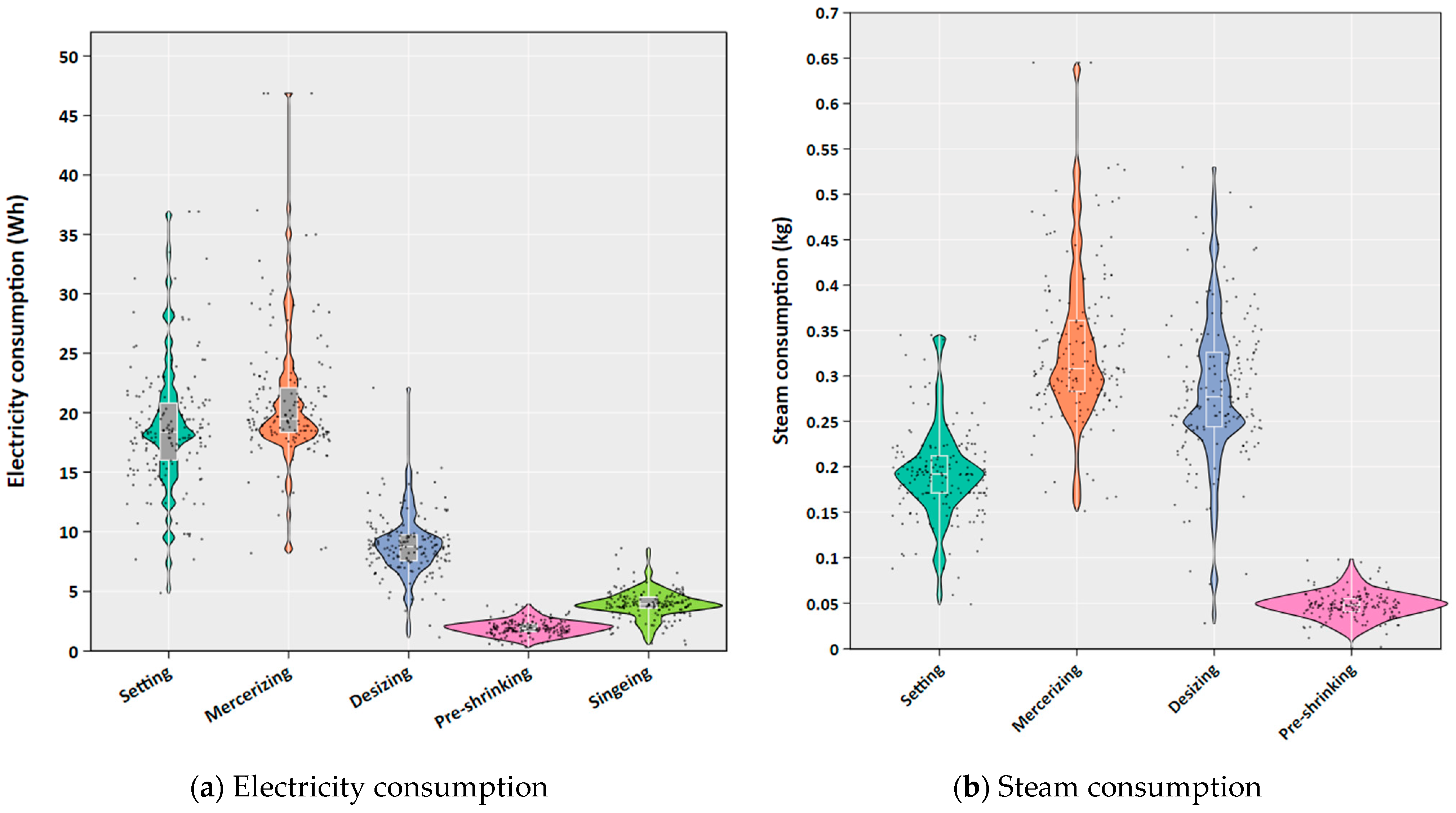
To enable equitable cross-process CF comparison, our analysis specifically focused on 175 products that completed a standardized finishing sequence comprising singeing, desizing, mercerizing, setting, and pre-shrinking operations. Products with partial finishing routes were excluded from this comparative analysis to maintain methodological consistency. Figure 2 illustrates that the mercerizing, setting, and desizing processes exhibit significant electricity consumption per unit of output, followed by singeing and pre-shrinking, which align with the equipment’s active power value. Steam usage per unit of product follows the sequence of mercerizing, desizing, setting, and pre-shrinking, whereas the singeing process does not utilize steam.

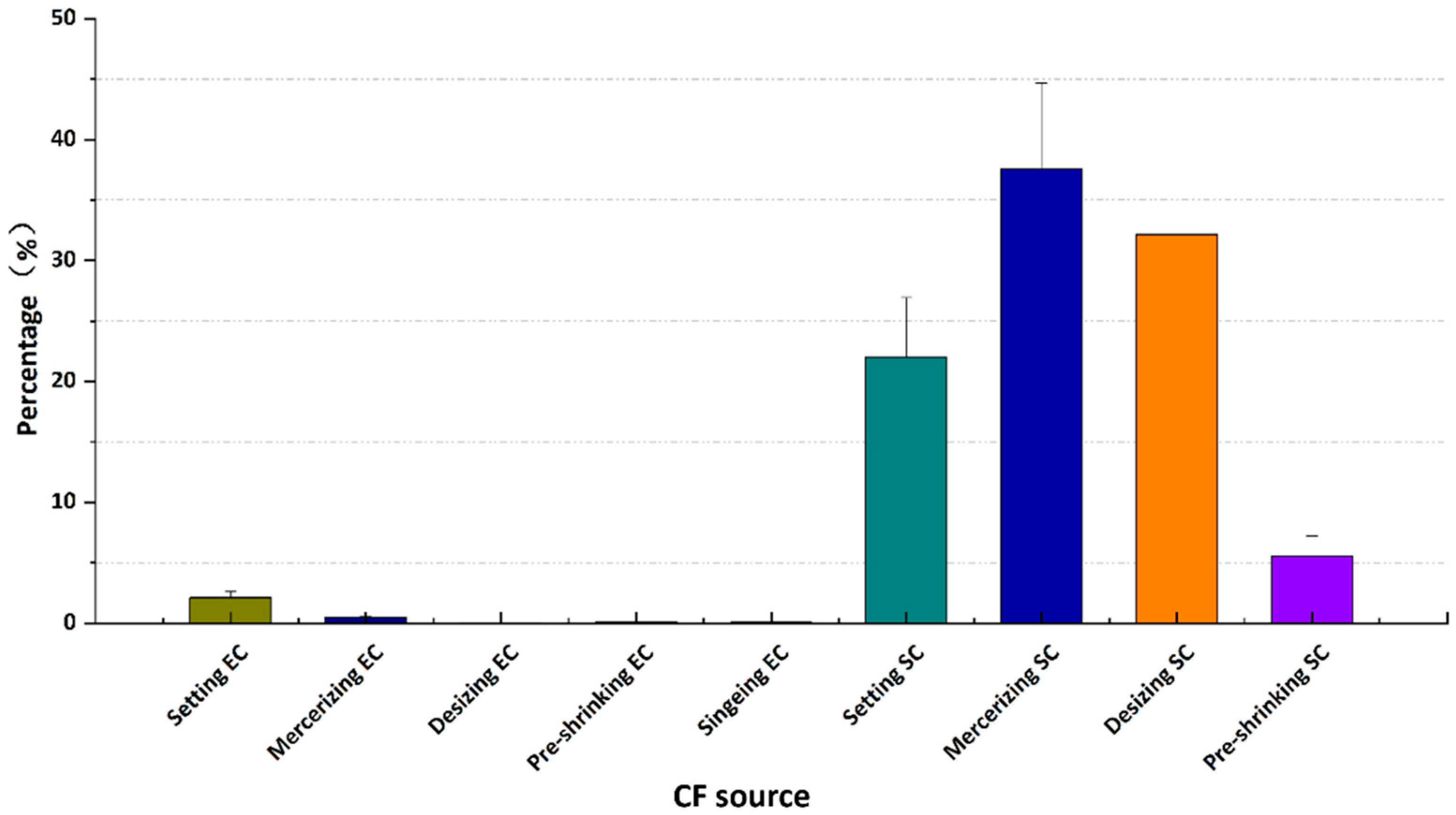
Figure 3 illustrates the ratio of the CF produced by the energy consumption of each process to the CF per unit of product. The CF per unit product is predominantly attributed to steam usage (97.24%), while the contribution from electricity consumption is minimal at only 2.76%. Regarding CF per unit product, mercerizing steam consumption produces the highest CF (37.55 ± 7.13)%, followed by desizing steam consumption (32.17 ± 6.90)%, setting steam consumption (21.98 ± 4.96)%, and pre-shrinking steam consumption (5.54 ± 1.66)%. The remaining processes contribute less than 5% to the total electricity consumption, indicating that steam consumption is the predominant factor in the CF per unit product for steam-consuming processes. Consequently, steam-utilizing processes play a significant role in the CF per unit of product, and the primary determinants of steam consumption in each process substantially affect the CF value per unit of output.

4.2. Comparison with Other Cases

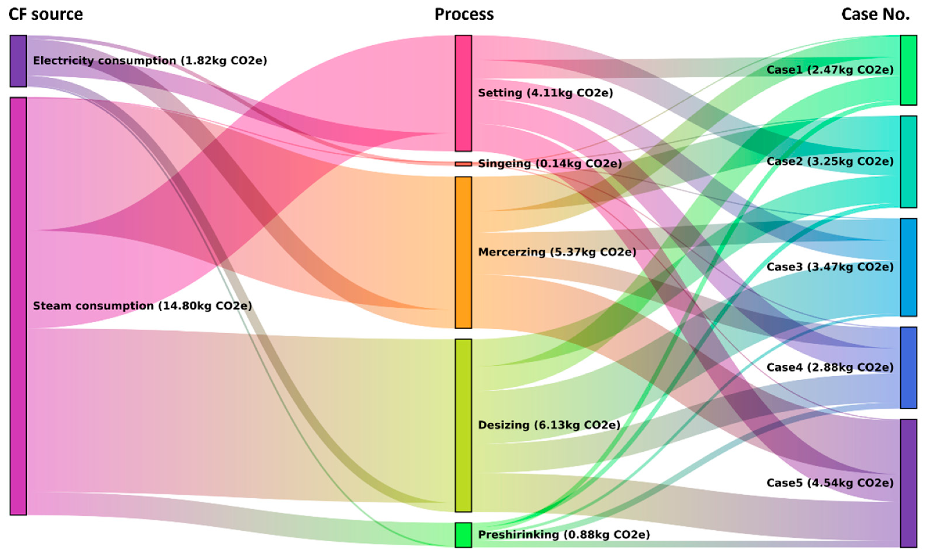
To elucidate the contribution of different sources to the CF in the finishing stage, thorough comparisons were performed between the results of this investigation and findings from previous studies. The comparisons involved the selected cases, including two cases from Turkey [14], one case from Indonesia [67], one case from Bangladesh [68]. Notably, Cases 1, 2, 3, 4, and 5 employed mercerized finishing, mercerized and silky finishing, mercerized and liquid ammonia, mercerized, liquid ammonia wrinkle-free (moisture cure) and silk protein techniques, respectively. While Cases A, B, C, and D from the other literature did not specify the post-processing method used.

Table 3. Comparison of CF from Cases 1, 2, 3, 4, 5, A, B, C, and D.

Case No.:	Type of Finishing	Electricity		Steam		Natural Gas		Oil		Total kg CO2e/kg
		kg CO2e/kg	%	kg CO2e/kg	%	kg CO2e/kg	%	kg CO2e/kg	%
1	Mercerized finishing	0.2850	11.53	2.1874	88.47	/	/	/	/	2.4724
2	Mercerized and silky finish	0.3797	11.68	2.8717	88.32	/	/	/	/	3.2514
3	Mercerized and liquid ammonia	0.3613	10.42	3.1055	89.58	/	/	/	/	3.4668
4	Mercerized and tapping	0.3097	10.74	2.539	89.26	/	/	/	/	2.8835
5	Mercerized, liquid ammonia wrinkle-free (moisture-cure) and silk protein	0.4841	10.65	4.0593	89.35	/	/	/	/	4.5434
A	Woven fabric final finishing	0.108	5.68	1.729	91.00	0.063	3.32	/	/	1.900
B	Knitted fabric finishing	0.490	7.62	5.939	92.38	/	/	/	/	6.429
C	Knitted fabrics finishing	0.8633	23.91	2.7468	76.09	/	/	/	/	3.6101
D	T-shirt fabrics finishing	0.1746	34.20	/	/	0.3345	65.52	0.0014	2.79	0.5106

presents the comparative data of CF from these other investigations, and the CF pathways for different subsections in the finishing phases are provided in Figure 4. All cases examined in this analysis involved 100% cotton textile products and the CF results have been standardized to a functional unit(kg) textile products to ensure equitable comparison across studies.

The comparative analysis indicates a notable discrepancy: the CF from the five Chinese cases, two Turkish cases, and one Indonesian case were more than five times the value of the Bangladesh case. Specifically, the CF in case B was 6.429 kg CO₂e/kg. Notably, the electricity and steam usage patterns between the cases were quite similar (natural gas was used for steam generation in Case D). Notwithstanding variations in finishing type, the differences in CF were negligible. This suggests that the CF during the finishing stage may not be significantly affected by the finishing type. In general, the CF associated with steam consumption generally exceeded that linked to electricity consumption, accounting for 76.09% to 92.38%. Therefore, it is essential to focus on emissions linked to steam consumption in the finishing stage. The dominance of steam consumption identified in this study underscores the critical importance of targeting thermal energy use for meaningful emissions reduction. Several technological innovations offer promising pathways for decarbonization. Heat recovery systems, such as economizers and heat exchangers, can capture waste heat from exhaust streams and process cooling water, potentially reducing steam demand. Furthermore, transitioning to renewable steam generation represents a transformative opportunity. Biomass boilers, solar thermal arrays, and green hydrogen-based systems can progressively displace fossil-fuel-derived steam. The integration of these technologies, combined with energy efficiency measures like automated steam trap maintenance and optimized insulation, could reduce the CF of textile finishing by 40–70% while maintaining product quality [14]. The result for Case 4 also indicates that using natural gas indeed reduces the CF.

Two key factors drive CF discrepancies across cases. Steam dominates CF (76.09–92.38% of total), and low-carbon fuels (e.g., biomass in Indonesia, natural gas with heat recovery in Bangladesh) reduce CF by 10–40% compared to coal-based steam in our Chinese cases. Furthermore, coal-dominated grids in China (0.86 kg CO₂e/kWh) lead to higher electricity-related CF (10.42–11.68%) than Turkey’s emission factor (0.478 kg CO₂e/kWh, 8.8% electricity CF) or Bangladesh’s emission factor (0.637 kg CO₂e/kWh, 7.6% electricity CF). In terms of global alignment, our cases match the global average for cotton textiles according to the current report [69].

4.3. Correlation Factor Analysis for Energy Consumption of Each Process

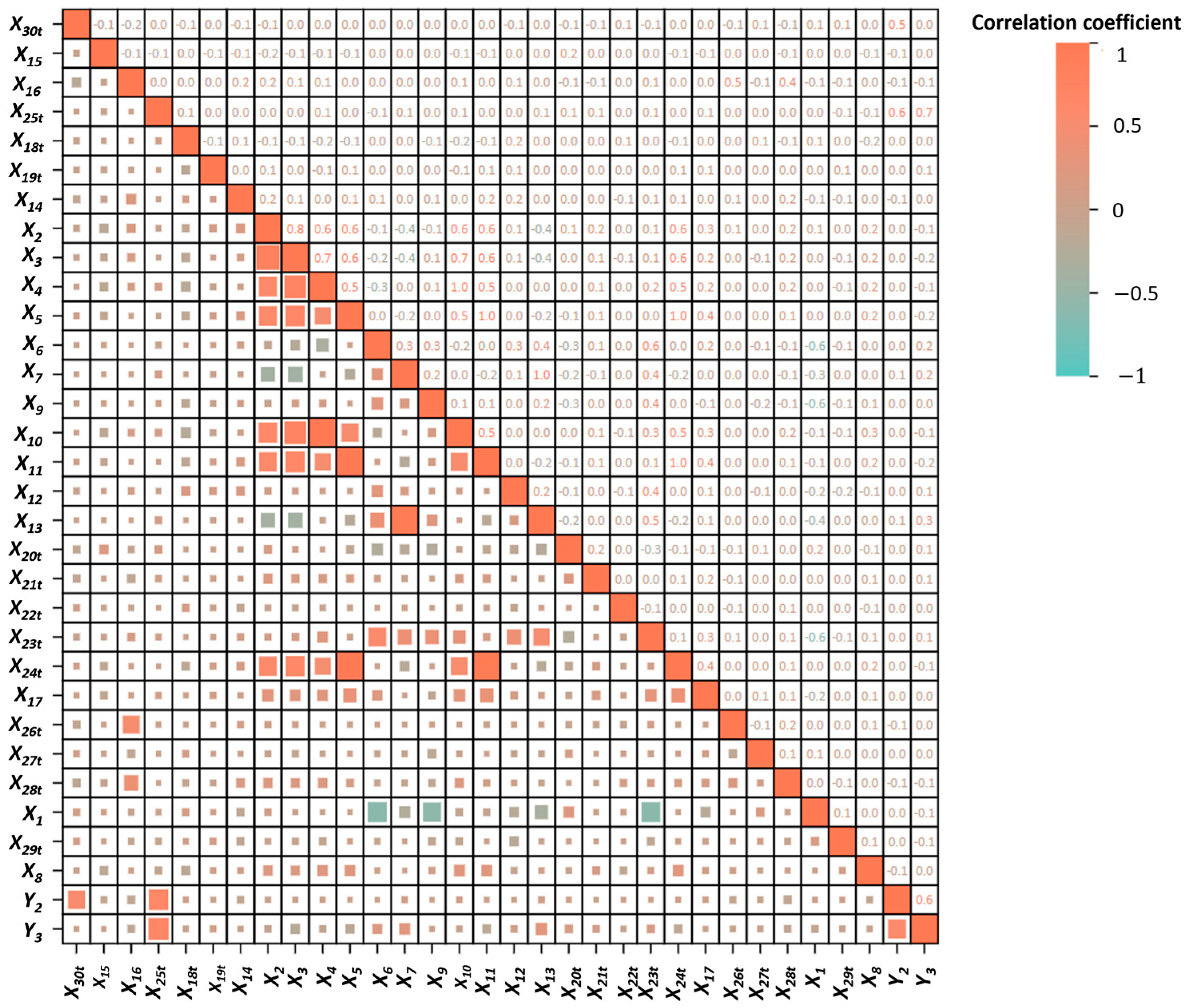
A comprehensive dataset encompassing relevant factors (shown in Supplementary Table S2) for each process across all 672 cases was analyzed. This study identified a total of 24 factors (referred to as X_1s to X_24s) for singeing process, 26 factors (referred to as X_1d to X_26d) for setting process, 26 factors (referred to as X_1y to X_26y) for pre-shrinking process, 28 factors (referred to as X_1w to X_28w)for washing process, 30 factors (referred to as X_1t to X_30t) for desizing process, 31 factors (referred X_1m to X_31m) for mercerizing process. To begin, the correlation between these 30 factors and desizing process electricity consumption (Y_2t) and steam consumption (Y_3t) was assessed, as illustrated in Figure 5.

The primary factors influencing electricity consumption, ranked by their correlation coefficient, are: job allowance ratio (0.64), average active power (0.54), fluorescence (−0.13), and color (−0.12). Job allowance ratio and average active power exhibit a significant positive linear correlation with power consumption, while fluorescence and color demonstrate a significant negative linear correlation with power consumption. The primary factors influencing steam consumption, listed in order of significance, are: job allowance ratio (0.69), mass per unit area of finished fabric (0.28), mass per unit area of gray fabric (0.25), weft yarn fineness (−0.20), gray fabric width (0.19), weft density of gray fabric (−0.16), weft density of finished product (−0.15), weft density of drop cloth (−0.15), average width of drop cloth (0.13), machine speed (0.13), color (−0.10), fluorescence (−0.09), machine temperature(0.09) and composition (−0.09). This indicates significant multicollinearity among the independent variables, as well as between the dependent variables. These variables are not entirely independent.

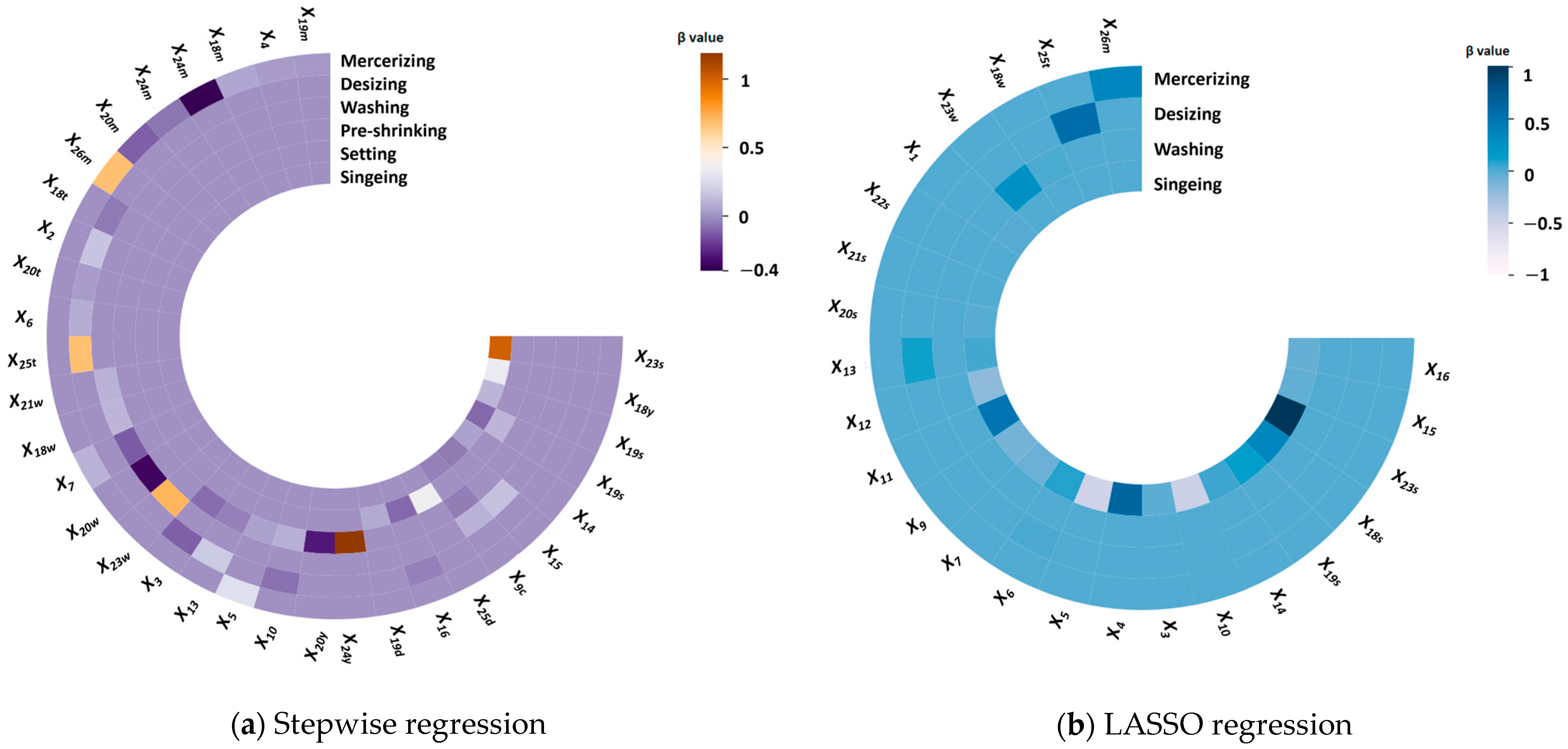
In such scenarios, stepwise regression and LASSO regression analysis can be employed to identify the factors impacting the dependent variables, and the results are shown in Supplementary Table S3. Different factor screening methodologies yield varying results. In the majority of processes, the absolute value of the β estimate for the job allowance ratio is the highest, with all values exceeding 0. This indicates that an increase in the job allowance ratio correlates with heightened electricity and steam consumption. Conversely, the machine speed in process parameters is substantial, with all values being less than 0, indicating that greater speed results in reduced electricity and steam consumption. The results showed that the job allowance ratio exerting the most substantial impact on the consumption of electricity and steam.

4.4. Correlation Factor Analysis for CF of Each Process

Figure 6 presents the outcomes of stepwise regression and LASSO regression for the screening of factors influencing the CF of each process. The β value indicates that, for the majority of processes, the absolute values of the estimates for the job allowance ratio at the management level are the highest, all exceeding zero. This suggests that an increase in the job allowance ratio correlates with a larger CF per unit product. Conversely, a reduction in the job allowance ratio, alongside enhancements in staff efficiency and optimization of production scheduling, can significantly diminish the CF per unit product. The singeing process does not involve steam use and therefore, the assessment of the CF during combustion yields identical results to the evaluation of factors influencing electricity consumption.

Diverse factor screening methodologies yield varying results. A comparative analysis revealed discrepancies between the factor screening outcomes of LASSO regression and stepwise regression. Generally, the stepwise regression results support the observation that, across most processes, the absolute value of the β value for the job allowance ratio is the highest and consistently positive. This indicates that a higher job allowance ratio correlates with an increased CF per unit of product. This suggests that an increase in the job allowance ratio correlates with a greater CF per unit of product. Analysis of stepwise regression indicates that the primary influencing factors for most processes are the job allowance ratio, and the machine speed of process parameters.

4.5. Predictive Model Comparison

Utilizing the factors affecting the CF of the six finishing processes as input variables, prediction models including PCR, PLSR, GA-ELM, PSO-ELM, GA-SVR, and PSO-SVR were developed to forecast the CF of these processes. Since not all models are equally suitable for predicting the CF, it is essential to accurately assess the performance of the six prediction models using both training and test samples to determine their respective strengths and weaknesses, and subsequently select the optimal model for predicting process-level CF. The performance of the six predictive models was evaluated based on R², RMSE, and SMAPE, with results validated by five-fold cross-validation (as illustrated in Supplementary Table S4).

4.5.1. Comparison of the R² for the Prediction Model

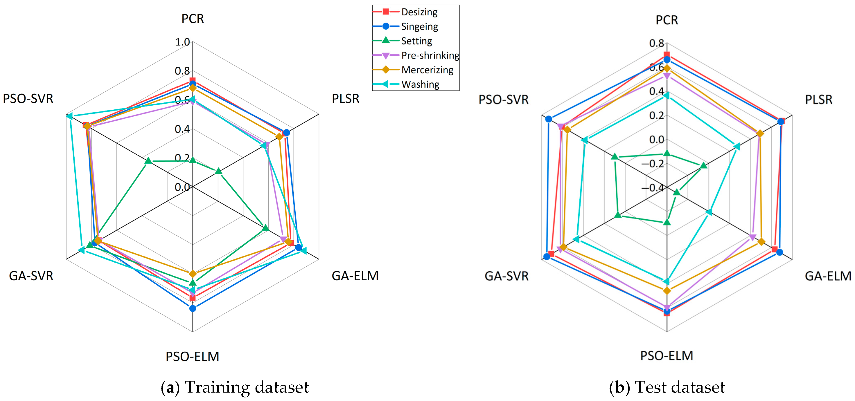
The radar charts for the CF training and test samples were illustrated, as depicted in Figure 7. Figure 7a presents the R² of the CF prediction model for the training dataset, whereas Figure 7b displays the R² for the test dataset. It illustrates that during the training samples, the R² values of the CF prediction models for the desizing, singeing, pre-shrinking, mercerizing, and washing processes were high. Notably, the desizing and singeing processes exhibited the highest R² values, ranging from 0.7 to 0.85, while the setting process had the lowest R². For the test dataset, the desizing and singeing processes exhibited the highest R², ranging from 0.6 to 0.8, followed by the mercerizing and pre-shrinking processes (0.5 to 0.6). The washing process had an R² between 0.3 and 0.5, while the R² for the setting process was predominantly below 0, indicating a poor model fit. For the training dataset, the PSO-SVR CF prediction model exhibited the highest R², followed by the GA-SVR model. The GA-ELM and PSO-ELM models performed worse than the SVR models but better than the PCR and PLSR models. In the test dataset, the GA-SVR model again demonstrated the highest R², followed by the PSO-SVR model, with the PCR and PLSR models performing worse. The PCR and PLSR models are inferior to the SVR model, while superior to the ELM model.

4.5.2. Comparison of the RSME for the Prediction Model

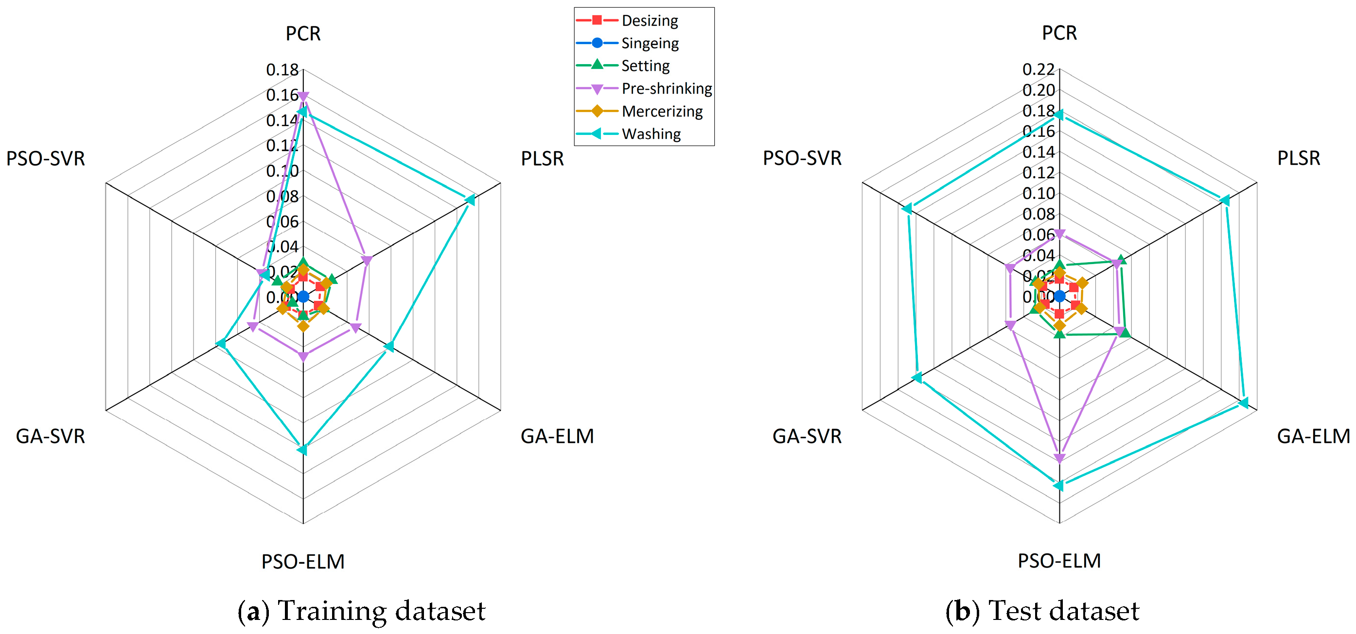
The radar maps for the CF training and test samples were illustrated, as depicted in Figure 8. Figure 8a presents the RMSE of the CF prediction model for the training dataset, whereas Figure 8b displays the RMSE for the test dataset. Figure 8 demonstrates that the RMSE of the CF prediction model for the washing and pre-shrinking processes was higher in both the training and test dataset. The RMSE for the mercerizing, desizing, and setting processes was moderate, while the RMSE for the singeing process was the lowest. Among the predictive models, the PSO-SVR model had the lowest RMSE during the training dataset, followed by the GA-SVR model. The ELM models demonstrated lower performance relative to the SVR models but outperformed the PCR and PLSR models. During the test dataset, the GA-SVR model demonstrated the lowest RMSE, followed by the PSO-SVR model. The PCR and PLSR models exhibited lower performance than the SVR models but better performance than the ELM models.

4.5.3. Comparison of the SMAPE for the Prediction Model

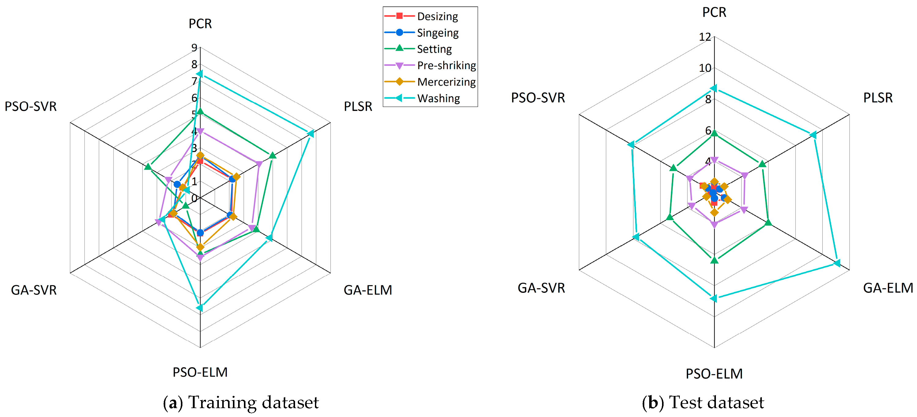
The radar maps for the CF training and test samples were illustrated, as depicted in Figure 9. Figure 9a presents the CF prediction model SMAPE for the training dataset, whereas Figure 9b demonstrates the same for the test dataset. Figure 9 demonstrates that, during the training dataset, the SMAPE of the CF prediction model for the desizing, singeing, pre-shrinking, mercerizing, and setting processes was below 10%. While the washing process exhibited the highest SMAPE, indicating the largest model error. The CF prediction models for the desizing, singeing, and mercerizing processes had the lowest error, with SMAPE below 3%. In contrast, the other processes—pre-shrinking, setting, and washing—demonstrated higher error rates, in increasing order. Among the predictive models, the PSO-SVR model had the lowest SMAPE during the training phase, followed by the GA-SVR model. The GA-ELM and PSO-ELM models exhibited worse performance than the SVR models but outperformed the PCR and PLSR models. During the test dataset, the GA-SVR model exhibited the lowest SMAPE, followed by the PSO-SVR model. The PCR and PLSR models demonstrated higher SMAPE than the SVR models but lower SMAPE than the ELM models.

4.5.4. Comparison Results of the Prediction Model

In conclusion, the aforementioned comparison allows for the following inferences to be drawn:

(1)

The R² during the training phase demonstrated suboptimal performance for some processes due to the limited dataset (e.g., 206 samples for setting process), the lack of data for specific equipment parameters, and the exclusion of certain equipment-related factors from the input variables. Factor screening identified equipment-related parameters as substantial contributors to the CF. Consequently, the regression prediction models for some processes exhibited lower fitting accuracy. The SMAPE for the washing process was the highest, likely due to the limited number of samples and the inherent variability in the process. The limited number of training samples for certain processes may lead to inadequate model training, and the test samples might also be insufficient or unevenly distributed.

(2)

The SVR approach demonstrated superior performance compared to PCR, PLSR, and ELM in terms of R², RMSE, and SMAPE. Among the SVR methods, the GA-SVR approach exhibited the best performance, while the PSO-SVR approach was slightly inferior. In most cases, the GA-SVR method achieved the lowest RMSE and SMAPE values, along with the highest R² value. This finding suggests that the GA-SVR model provides a better fit and generates smaller prediction errors compared to the other methods. Consequently, the GA-SVR model is recommended for predicting the CF at the process level.

5. Conclusions

This study establishes a process-level CF calculation model and calculates the finishing-stage carbon emissions for the case of 672 textile products. By summarizing and generalizing the influencing factors in the literature review, the influencing factors can be classified into products, production environment, production process, management level, and processing equipment. The influencing factors were identified through correlation analysis. Additionally, this study developed several machine learning-based predictive models, including PCR, PLSR, GA-ELM, PSO-ELM, GA-SVR, and PSO-SVR. The research findings are summarized as follows:

(1)

For electricity consumption per unit product, the mercerizing, setting, and desizing processes are relatively high, followed by singeing and preshrinking, which aligns with the trend of the equipment’s active power. As for steam consumption per unit product, the order from highest to lowest is mercerizing, desizing, setting, and preshrinking, while the singeing process does not use steam. The CF per unit product is almost entirely derived from steam consumption (97.24%), with electricity consumption contributing only 2.76%. Therefore, processes involving steam consumption play a dominant role in the CF per unit product, and the main factors affecting steam consumption in each process significantly influence the CF value per unit product.

(2)

For most processes, the main influencing factors are the job allowance ratio and the machine speed. The job allowance ratio has the most significant impact on electricity, steam consumption and CF.

(3)

Among the studied manufacturing processes, the regression prediction model demonstrated the poorest performance for the setting process, while the washing process exhibited the largest prediction errors. Comparative analysis of the modeling methods revealed that SVR consistently outperformed PCR, PLSR, and ELM. Notably, the GA-SVR approach showed superior performance across most processes, achieving simultaneously the lowest RMSE and SMAPE, along with R². These results indicate that the GA-SVR model provides better fitting accuracy and smaller prediction errors compared to alternative methods. Consequently, the GA-SVR model is recommended for accurate prediction of CF at the individual process level in manufacturing systems.

The practical innovation contributions of this research can be summarized as follows: Firstly, this study pioneered the development of a process-level CF calculation model for textile finishing processes. The model systematically delineates emission profiles across manufacturing processes using empirical data from 672 textile goods. Determining essential intervention points for emission reduction in textile production. Secondly, we developed a hierarchical factor analysis approach that includes product qualities, production environment, process parameters, management variables, and equipment specifications through rigorous literature study and correlation analysis. The paper presents initial evidence that the job allowance ratio strongly influences both energy consumption and CF, providing novel theoretical insights for process-level carbon management. We created six machine learning optimization models, including GA-SVR and PSO-SVR. Comparative investigations have shown that GA-SVR achieves superior performance in predicting process-level CF, hence offering a dependable analytical instrument for process-level carbon management in manufacturing systems. The quantitative findings of this study provide critical data-driven guidance for formulating industrial decarbonization policies. Specifically, the dominance of steam consumption (97.24%) in the CF of textile finishing underscores the paramount importance of transitioning to renewable steam generation and establishing mandatory energy efficiency standards for the finishing process. The identified key influencing factors, particularly the job allowance ratio and the machine speed, offer concrete technical pathways for optimizing production scheduling and equipment operation to reduce CF.

This study has created a solid framework for assessing the CF at the process level in China’s textile sector. Nevertheless, additional validation and adaptation are required to improve its worldwide relevance. The suggested GA-SVR model exhibits robust predictive performance under Chinese production circumstances. However, its efficacy must be validated across diverse regional contexts and more extensive textile manufacturing processes, especially considering viscose finishing technologies. Due to the intricate global supply chains of the textile industry, which involve production across various countries with differing environmental regulations and technological capacities, it is essential to apply this methodology to international partners, especially small and medium-sized enterprises that do not possess sophisticated monitoring systems. Future research should concentrate on: (1) prioritizing the integration of advanced material characterization and environmental monitoring. Specifically, quantifying coating formulations and impregnation chemistry, along with measuring ventilation dynamics through anemometry, would significantly improve model accuracy by capturing currently unmeasured physicochemical and thermodynamic factors; (2) creating a cloud-based modular assessment tool to enable swift CF calculations without necessitating onsite audits; (3) enhancing the reusability of process-level emission modules to reduce redundant data collection; (4) incorporating blockchain or IoT-enabled real-time data for dynamic carbon tracking. The creation of standardized, shareable CF unit databases could substantially alleviate assessment requirements for worldwide supply chain stakeholders. Beyond the textile sector, the GA-SVR model developed here holds significant promise for cross-sectoral applications. The model’s ability to handle complex, non-linear relationships between operational parameters and CF makes it adaptable to other energy-intensive manufacturing industries, such as pulp and paper, food processing, or chemical production. These sectors share similar characteristics in thermal energy consumption and process variability. This convergence of industrial characteristics thereby establishes a robust foundation for extending this methodological framework to advance carbon management practices across industrial ecosystems.

References

1. Imran, S.; Mujtaba, M.; Zafar, M.M.; Hussain, A.; Mehmood, A.; Farwa, U.E.; Korakianitis, T.; Kalam, M.; Fayaz, H.; Saleel, C.A. Assessing the potential of GHG emissions for the textile sector: A baseline study. Heliyon 2023, 9, e22404. [Google Scholar] [CrossRef]
2. Sharpe, S.; Dominish, E.; Martinez-Fernandez, M.C. Taking Climate Action: Measuring Carbon Emissions in the Garment Sector in Asia; ILO Working Paper: Geneva, Switzerland, 2022. [Google Scholar]
3. Notarnicola, B.; Sala, S.; Anton, A.; McLaren, S.J.; Saouter, E.; Sonesson, U. The role of life cycle assessment in supporting sustainable agri-food systems: A review of the challenges. J. Clean. Prod. 2017, 140, 399–409. [Google Scholar] [CrossRef]
4. Pandey, D.; Agrawal, M.; Pandey, J.S. Carbon footprint: Current methods of estimation. Environ. Monit. Assess. 2011, 178, 135–160. [Google Scholar] [CrossRef]
5. Muthu, S.S. Environmental Footprints and Eco-Design of Products and Processes; SGS Hong Kong Limited: Hong Kong, China, 2016. [Google Scholar]
6. Huynh, N.-T.; Chien, C.-F. A hybrid multi-subpopulation genetic algorithm for textile batch dyeing scheduling and an empirical study. Comput. Ind. Eng. 2018, 125, 615–627. [Google Scholar] [CrossRef]
7. Savin, I.-I.; Butnaru, R. Wastewater characteristics in textile finishing mills. Environ. Eng. Manag. J. 2008, 7, 859–864. [Google Scholar] [CrossRef]
8. Peng, M.; Liu, C.; Chen, S.; Gao, S.; Jiang, L.; Ma, J. Development and performance study of a new shrink-proof and non-iron cotton blended fabric. Text. Res. J. 2018, 89, 3269–3279. [Google Scholar] [CrossRef]
9. Kumar, V.; Koehl, L.; Zeng, X.; Ekwall, D. Coded yarn based tag for tracking textile supply chain. J. Manuf. Syst. 2017, 42, 124–139. [Google Scholar] [CrossRef]
10. Cheng, Y.; Liang, H.-E. Calculation and evaluation of industrial carbon footprint of cotton denim jacket. J. Eng. Fibers Fabr. 2021, 16, 15589250211020387. [Google Scholar] [CrossRef]
11. Dominish, E.; Sharpe, S. Reducing the Footprint? How to Assess Carbon Emissions in the Garment Sector in Asia; International Labour Organization: Geneva, Switzerland, 2021. [Google Scholar]
12. Jain, M. Ecological approach to reduce carbon footprint of textile industry. Int. J. Appl. Home Sci. 2017, 4, 623–633. [Google Scholar]
13. Costa, I.; Martins, F.; Alves, I. Ecological Footprint as a sustainability indicator to analyze energy consumption in a Portuguese textile facility. Int. J. Energy Environ. Eng. 2019, 10, 523–528. [Google Scholar] [CrossRef]
14. Dal, A.; Yesil, E.S.; Ozturk, E.; Kitis, M. Investigation of water and carbon footprint reductions employing best available techniques in the textile sector. J. Clean. Prod. 2024, 466, 142913. [Google Scholar] [CrossRef]
15. Muthu, S.S.; Gardetti, M.A. Sustainability in the Textile and Apparel Industries; Springer: Berlin/Heidelberg, Germany, 2020. [Google Scholar]
16. Mikucioniene, D.; Mínguez-García, D.; Repon, M.R.; Milaius, R.; Priniotakis, G.; Chronis, I.; Kiskira, K.; Hogeboom, R.; Belda-Anaya, R.; Díaz-García, P. Understanding and addressing the water footprint in the textile sector: A review. AUTEX Res. J. 2024, 24, 20240004. [Google Scholar] [CrossRef]
17. Li, Y.; Yang, X.; Du, E.; Liu, Y.; Zhang, S.; Yang, C.; Zhang, N.; Liu, C. A review on carbon emission accounting approaches for the electricity power industry. Appl. Energy 2024, 359, 122681. [Google Scholar] [CrossRef]
18. Li, X.; Ren, J.; Wu, Z.; Wu, X.; Ding, X. Development of a novel process-level water footprint assessment for textile production based on modularity. J. Clean. Prod. 2021, 291, 125884. [Google Scholar] [CrossRef]
19. Uddin, F. Introductory chapter: Textile manufacturing processes. In Textile Manufacturing Processes; IntechOpen: London, UK, 2019. [Google Scholar]
20. Fonseca, A.; Ramalho, E.; Gouveia, A.; Henriques, R.; Figueiredo, F.; Nunes, J. Systematic Insights into a Textile Industry: Reviewing Life Cycle Assessment and Eco-Design. Sustainability 2023, 15, 15267. [Google Scholar] [CrossRef]
21. Selli, F.; Şen, K.; Kaya, A.; Erdoğan, Ü.H. Effect of Reprocess on the Sustainability of T-Shirt Production. Tekst. Ve Mühendis 2022, 29, 70–80. [Google Scholar]
22. Zhang, S.; Xu, C.; Xie, R.; Yu, H.; Sun, M.; Li, F. Environmental assessment of fabric wet processing from gate-to-gate perspective: Comparative study of weaving and materials. Sci. Total Environ. 2023, 857, 159495. [Google Scholar] [CrossRef] [PubMed]
23. Wang, C.; Wang, L.; Liu, X.; Du, C.; Ding, D.; Jia, J.; Yan, Y.; Wu, G. Carbon footprint of textile throughout its life cycle: A case study of Chinese cotton shirts. J. Clean. Prod. 2015, 108, 464–475. [Google Scholar] [CrossRef]
24. Moreira, N.; de Santa-Eulalia, L.A.; Aït-Kadi, D.; Wood–Harper, T.; Wang, Y. A conceptual framework to develop green textiles in the aeronautic completion industry: A case study in a large manufacturing company. J. Clean. Prod. 2015, 105, 371–388. [Google Scholar] [CrossRef]
25. Onlu, N. Sustainability by design in textile products and fashion. New Des. Ideas 2017, 1, 37–49. [Google Scholar]
26. van der Voet, E. Books: Our Ecological Footprint: Reducing Human Impact on the Earth; Wiley Online Library: Hoboken, NJ, USA, 1999. [Google Scholar]
27. Wiedmann, T.; Minx, J. A definition of ‘carbon footprint’. Ecol. Econ. Res. Trends 2008, 1, 1–11. [Google Scholar]
28. ISO 14067: 2018; Greenhouse Gases—Carbon Footprint of Products-Requirements and Guidelines for Quantification. International Organization for Standardization: Geneva, Switzerland, 2018.
29. PAS 2050: 2011; Specification for the Assessment of the Life Cycle Greenhouse Gas Emissions of Goods and Services. British Standards Institution: London, UK, 2011.
30. Long, Y.; Yoshida, Y.; Liu, Q.; Zhang, H.; Wang, S.; Fang, K. Comparison of city-level carbon footprint evaluation by applying single-and multi-regional input-output tables. J. Environ. Manag. 2020, 260, 110108. [Google Scholar] [CrossRef]
31. Penaloza, D.; Erlandsson, M.; Berlin, J.; Wålinder, M.; Falk, A. Future scenarios for climate mitigation of new construction in Sweden: Effects of different technological pathways. J. Clean. Prod. 2018, 187, 1025–1035. [Google Scholar] [CrossRef]
32. ISO 14040: 2006; Environmental Management—Life Cycle Assessment-Principles and Framework. International Organization for Standardization: Geneva, Switzerland, 2006.
33. Liu, C.; Li, X.; Li, Q.; Chen, Y.; Liu, J.; Liu, S.; Wang, L. Carbon footprint calculation and evaluation of mulberry silk quilts. Text. Res. J. 2024, 95, 471–484. [Google Scholar] [CrossRef]
34. Bianco, I.; Picerno, G.; Blengini, G.A. Life Cycle Assessment (LCA) of Worsted and Woollen processing in wool production: ReviWool® noils and other wool co-products. J. Clean. Prod. 2023, 415, 137877. [Google Scholar] [CrossRef]
35. Li, C.; Zhang, T.; Zhou, X.; Cheng, Z.; Xu, T.; Li, Z.; Hong, J. Carbon–water–energy footprint impacts of dyed cotton fabric production in China. J. Clean. Prod. 2024, 467, 142898. [Google Scholar] [CrossRef]
36. Kılıç, E.; McLaren, S.J.; Holmes, G.; Fullana-i-Palmer, P.; Puig, R. Product environmental footprint of New Zealand leather production. Int. J. Life Cycle Assess. 2023, 28, 349–366. [Google Scholar] [CrossRef]
37. Liu, J.; Li, X.; Zhang, Y.; Sun, L.; Huang, Q.; Zhu, L.; Wang, L. Carbon footprint and oxygen footprint assessment of hemp yarn. Int. J. Glob. Warm. 2024, 32, 361–373. [Google Scholar] [CrossRef]
38. Luo, Y.; Wu, X.; Ding, X. Carbon and water footprints assessment of cotton jeans using the method based on modularity: A full life cycle perspective. J. Clean. Prod. 2022, 332, 130042. [Google Scholar] [CrossRef]
39. Li, Z.; Zhou, Y.; Zhao, M.; Guan, D.; Yang, Z. The carbon footprint of fast fashion consumption and mitigation strategies-a case study of jeans. Sci. Total Environ. 2024, 924, 171508. [Google Scholar] [CrossRef]
40. Chen, B.; Qian, W.; Yang, Y.; Liu, H.; Wang, L. Carbon footprint and water footprint of cashmere fabrics. Fibres Text. East. Eur. 2021, 4, 94–99. [Google Scholar] [CrossRef]
41. Chen, Y.; Bi, Y.; Wu, X.; Ding, X. Impact of additional carbon storage of natural plant fiber on product carbon footprint: A case study of cotton/kapok blended T-shirt VS pure cotton T-shirt. J. Clean. Prod. 2024, 434, 140237. [Google Scholar] [CrossRef]
42. Zhu, D.; Bao, Y.; Ding, X.; Wu, X. Unveil the carbon footprint of textiles dyed with different reactive dyestuff recipes from an industrial manufacturing perspective. Int. J. Life Cycle Assess. 2024, 29, 1598–1620. [Google Scholar] [CrossRef]
43. Qian, W.; Ji, X.; Xu, P.; Wang, L. Carbon footprint and water footprint assessment of virgin and recycled polyester textiles. Text. Res. J. 2021, 91, 2468–2475. [Google Scholar] [CrossRef]
44. He, B.; Duan, H.; Yang, W.; Yabar, H.; Song, J. Decarbonizing polyamide textile production in China: Footprints and mitigation pathways from life cycle perspective. Resour. Conserv. Recycl. 2024, 208, 107705. [Google Scholar] [CrossRef]
45. Gomez-Campos, A.; Vialle, C.; Rouilly, A.; Sablayrolles, C.; Hamelin, L. Flax fiber for technical textile: A life cycle inventory. J. Clean. Prod. 2021, 281, 125177. [Google Scholar] [CrossRef]
46. Li, D.; Feng, S.; Tao, J.; Yu, S.; He, Y.; Yu, R.; Xiang, H.; Wang, C.; Zhu, M. Optimizing Sustainability in Textile Recycling: Life Cycle Assessment of Recycled Polyester Staple Fibers with a Focus on Carbon Emissions, Energy Efficiency, and Water Conservation. ACS Sustain. Chem. Eng. 2024, 12, 17347–17356. [Google Scholar] [CrossRef]
47. Suarez, A.; Ford, E.; Venditti, R.; Kelley, S.; Saloni, D.; Gonzalez, R. Rethinking the use of bio-based plastics to accelerate the decarbonization of our society. Resour. Conserv. Recycl. 2022, 186, 106593. [Google Scholar] [CrossRef]
48. Angelis-Dimakis, A.; Whitehouse, A.; Vyrkou, A.; Hebden, A.; Rana, S.; Goswami, P. Life cycle environmental impact and economic assessment of British Wool face masks. Clean. Environ. Syst. 2022, 6, 100084. [Google Scholar] [CrossRef]
49. Hasanbeigi, A.; Price, L. A review of energy use and energy efficiency technologies for the textile industry. Renew. Sustain. Energy Rev. 2012, 16, 3648–3665. [Google Scholar] [CrossRef]
50. Pérez, L.A.E.; Pérez, A.T.E.; Vásquez, Ó.C. Exploring an alternative to the Chilean textile waste: A carbon footprint assessment of a textile recycling process. Sci. Total Environ. 2022, 830, 154542. [Google Scholar] [CrossRef] [PubMed]
51. Wang, S.; Chong, C.; Huang, W.; Guo, S.; Wang, Y.; Zhang, Y.; Pan, Z.; Wang, J.; Li, X.; Zhao, W. Tracing the carbon footprint of cotton garments from seed to garment: Evidence from an empirical study of multiple sites in China. Resour. Conserv. Recycl. 2025, 217, 108200. [Google Scholar] [CrossRef]
52. Moazzem, S.; Crossin, E.; Daver, F.; Wang, L. Environmental impact of apparel supply chain and textile products. Environ. Dev. Sustain. 2021, 24, 1–19. [Google Scholar] [CrossRef]
53. Mailley, D.; Hébraud, A.; Schlatter, G. A review on the impact of humidity during electrospinning: From the nanofiber structure engineering to the applications. Macromol. Mater. Eng. 2021, 306, 2100115. [Google Scholar] [CrossRef]
54. Fallahi, A.; Shahidi-Zadeh, B.; Niaki, S.T.A. Unrelated parallel batch processing machine scheduling for production systems under carbon reduction policies: NSGA-II and MOGWO metaheuristics. Soft Comput. 2023, 27, 17063–17091. [Google Scholar] [CrossRef]
55. Bashir, T.; Iftikhar, T.; Majeed, H. Bulk industrial textile production of bio scouring for cellulosic fabric utilizing indigenous hot springs triacylglycerol acylhydrolases from Bacillus toyonensis and Bacillus thuringiensis. Cellulose 2024, 31, 1353–1381. [Google Scholar] [CrossRef]
56. Xu, X.; Cui, X.; Zhang, Y.; Chen, X.; Li, W. Carbon neutrality and green technology innovation efficiency in Chinese textile industry. J. Clean. Prod. 2023, 395, 136453. [Google Scholar] [CrossRef]
57. Xiao, Q.; Li, C.; Tang, Y.; Chen, X. Energy efficiency modeling for configuration-dependent machining via machine learning: A comparative study. IEEE Trans. Autom. Sci. Eng. 2020, 18, 717–730. [Google Scholar] [CrossRef]
58. Nepal, B.; Yamaha, M.; Yokoe, A.; Yamaji, T. Electricity load forecasting using clustering and ARIMA model for energy management in buildings. Jpn. Archit. Rev. 2020, 3, 62–76. [Google Scholar] [CrossRef]
59. Asadi, M.; McPhedran, K.N. Greenhouse gas emission estimation from municipal wastewater using a hybrid approach of generative adversarial network and data-driven modelling. Sci. Total Environ. 2021, 800, 149508. [Google Scholar] [CrossRef]
60. Runge, J.; Zmeureanu, R. Forecasting energy use in buildings using artificial neural networks: A review. Energies 2019, 12, 3254. [Google Scholar] [CrossRef]
61. Wen, L.; Cao, Y. Influencing factors analysis and forecasting of residential energy-related CO2 emissions utilizing optimized support vector machine. J. Clean. Prod. 2020, 250, 119492. [Google Scholar] [CrossRef]
62. Ciulla, G.; D’Amico, A. Building energy performance forecasting: A multiple linear regression approach. Appl. Energy 2019, 253, 113500. [Google Scholar] [CrossRef]
63. Wang, Z.; Wang, Y.; Zeng, R.; Srinivasan, R.S.; Ahrentzen, S. Random Forest based hourly building energy prediction. Energy Build. 2018, 171, 11–25. [Google Scholar] [CrossRef]
64. T/CNTAC 11-2018; General Requirements for Quantifying the Greenhouse Gas Emissions of Textile Products. China National Textile and Apparel Council: Beijing, China, 2018.
65. Limb, J.; Rubinstein, C.; Thompson, J. Digital coding of color video signals-a review. IEEE Trans. Commun. 1977, 25, 1349–1385. [Google Scholar] [CrossRef]
66. Muqaddim, N.; Ahmed, S.; Azad, M.M. Impact of Work Study on Productivity: A Study on Athletic Shirt Manufacturing Process in the Apparel Industry. Int. J. New Technol. Res. 2021, 7, 23–29. [Google Scholar]
67. Dewi, R.G.; Parinderati, R.; Hendrawan, I.; Dewantoro, M.W.B.; Bayuwega, W.D. Energy Efficiency Monitoring in Textile Industries to Achieve GHG Emissions Reduction Target in Indonesia. In IOP Conference Series: Earth and Environmental Science; IOP Publishing: Bristol, UK, 2019; p. 012019. [Google Scholar]
68. Uddin, M.; Bhuiya, K.M.S.; Udoy, S.A.; Ahmed, M.M.; Hossan, M.N. Investigation of the energy consumption and emission for a readymade garment production and assessment of the saving potential. Energy Effic. 2024, 17, 100. [Google Scholar] [CrossRef]
69. Hasanbeigi, A. Energy-Efficiency Improvement Opportunities for the Textile Industry. 2010. Available online: https://www.energystar.gov/sites/default/files/buildings/tools/EE_Guidebook_for_Textile_industry.pdf (accessed on 7 November 2025).
Figure 2. Violin plot of electricity and steam consumption in each process. (a) Violin plots shows the distribution of electricity consumption (Wh per unit product) for each process. The plot width represents data density, with internal boxplots indicating the median (center line), interquartile range (box), and data range (whiskers). (b) Violin plots shows the distribution of steam consumption (Wh per unit product) for each process. The plot width represents data density, with internal boxplots indicating the median (center line), interquartile range (box), and data range (whiskers).
Sustainability 17 10350 g002
Figure 3. Percentage of CF generated by energy consumption per unit product in each process. The chart shows the percentage contribution of each process to the total CF, calculated from energy consumption data. Error bars represent standard deviation. EC represents electricity consumption and SC represents steam consumption.
Sustainability 17 10350 g003
Figure 4. CF pathways for different subsections in the finishing phases.
Sustainability 17 10350 g004
Figure 5. Correlation coefficient for factors affecting the desizing-process CF. The size of each box is proportional to the statistical significance level of the correlation.
Sustainability 17 10350 g005
Figure 6. Results of screening influential factors for stepwise regression and LASSO regression of the CF of each process.
Sustainability 17 10350 g006
Figure 7. The radar charts depict the R2 of the CF prediction model.
Sustainability 17 10350 g007
Figure 8. The radar charts of the RMSE of the prediction model of CF.
Sustainability 17 10350 g008
Figure 9. The radar charts of the SMAPE of the prediction model of CF.
Sustainability 17 10350 g009