Article

Prediction of Thermal and Oxidative Degradation of Amines to Improve Sustainability of CO2 Absorption Process

1
Centre for Engineering Innovation and Research, School of Engineering, Computing and Mathematical Sciences, University of Wolverhampton, Wolverhampton WV1 1LY, UK
2
School of Chemistry and Chemical Engineering, University of Surrey, Guildford GU2 7XH, UK
*
Author to whom correspondence should be addressed.
Sustainability 2025, 17(22), 10311; https://doi.org/10.3390/su172210311
Submission received: 12 September 2025 / Revised: 2 November 2025 / Accepted: 12 November 2025 / Published: 18 November 2025
(This article belongs to the Special Issue Carbon Capture, Utilization, and Storage (CCUS) for Clean Energy)

Abstract

Amine-based CO2 absorption is a leading technology for post-combustion carbon capture, but solvent degradation remains a critical barrier to its long-term sustainability. Degradation reduces capture efficiency, increases solvent make-up costs, and generates environmentally harmful by-products, undermining the viability of carbon capture as a sustainable climate mitigation strategy. This study applies advanced machine learning techniques—Artificial Neural Networks (ANN), Random Forest (RF), XGBoost, and Adaptive Neuro-Fuzzy Inference Systems (ANFIS)—to predict thermal and oxidative degradation of amine solvents under varying operating conditions. Experimental datasets for piperazine-based mixtures and tertiary amines were used to train and validate predictive models with high statistical accuracy. The results demonstrate that machine learning can reliably forecast degradation behaviour, reducing dependence on resource-intensive experimental campaigns and enabling more sustainable CO2 capture systems. By improving solvent stability assessment and process monitoring, this work contributes to the development of more resilient, cost-effective, and environmentally responsible carbon capture technologies, directly supporting global sustainability and climate change mitigation goals.

1. Introduction

CO2 absorption or solvent based carbon capture using amine solvents is recognised as the most established process for carbon capture globally. This process is the main scenario that has been considered to retrofit power plants, cement factories, chemical plants, and many other systems that can be categorised as post-combustion carbon capture technology. As shown in Figure 1, in this process, CO2 is absorbed in the absorber column, while the solvent is regenerated, and CO2 is released in the desorber/stripper column.
Amine solutions like Monoethanolamine (MEA) and Methyldiethanolamine (MDEA) exhibit drawbacks such as high energy consumption for solvent regeneration, susceptibility to degradation, amine emissions from top of the column, and corrosion issues [1]. Therefore, solvents can be lost by degradation and emissions from the system. Solvent losses in an absorption-stripping system can occur at multiple points in the system through different processes. As it shown in Figure 1, the red dashed line indicates regions in the absorption system where thermal degradation is dominant, while the blue dashed lines highlight the areas where oxidative degradation occurs. Oxidation is a chemical reaction between the amine and dissolved oxygen (O2) that enters the system with the flue gas. This reaction primarily takes place in the absorber sump, absorber packing, and the piping leading to the heat exchanger (the blue dashed area). Any remaining O2 after passing through the main cross exchanger will flash at the top of the stripper. In both the absorber and absorber sump, amine degradation due to oxidation is the main cause of solvent loss. Flue gas typically contains 3–5% O2, which is carried into the absorber where it reacts with the amine. Oxidation reactions typically cause the amine to break down into various degradation products, which can further react with each other, additional oxygen, or the amine itself, leading to the formation of even more degradation products in a complex series of reactions.
Thermal degradation occurs when an amine breaks down into degradation products due to exposure to high temperatures. In current designs, strippers operate in temperatures ranging from 100 to 120 °C, significantly higher than those in the absorber. At these elevated temperatures, degradation reactions that are suppressed in the absorber accelerate, leading to increased solvent losses. Thermal degradation primarily takes place in the stripper packing, stripper sump, reboiler, and reclaiming system (if used). It may also occur in the piping from the main cross-exchanger to the stripper if temperatures are sufficiently high. If a thermal reclaiming system is in place, the solvent is also exposed to high-temperature degradation in this stage.
The degradation compounds influence the CO2 absorption capacity, increasing corrosion, foaming, and fouling of the capture system. This has an economic impact where the operating costs related to amine degradation have been estimated to be around 10% of the total CO2 capture cost [2]. It is also reported that, based on the type of the solvent and application of the CO2 absorption system (flue gas, synthesis gas, or natural gas), thermal degradation will cost in the range of USD 0.06–0.26 per ton of captured CO2 [3]. Degradation products also impact health, safety, and the environment by releasing toxic and carcinogenic materials such as volatile components and nitrosamines [4].
The chemistry of amine degradation is complex. Thermal degradation occurs at elevated temperatures, typically through carbamate polymerisation and reactions between amines and CO2-derived species, leading to the formation of heat-stable salts and higher molecular-weight compounds. The degradation process begins with the reversible formation of carbamate intermediates, often following the six-membered CO2–amine interaction mechanism involving a nucleophilic attack of the amine on CO2. Under regeneration conditions, carbamate species can undergo intramolecular cyclisation to form 2-oxazolidinones and imidazolidinones, or condensation reactions yielding urea derivatives such as N-(2-hydroxyethyl)ethylenediamine (HEEDA) and triethylenetetramine (TETA). Further heating promotes decarboxylation and deamination steps that release light gases (CO2, NH3) and leave behind polymeric residues. Secondary amines such as diethanolamine (DEA) primarily degrade through β-elimination, while tertiary amines degrade via dealkylation pathways, forming alcohols and alkenes. Solvent type, CO2 loading, and residence time in the stripper directly influence the rate of these condensation and decomposition reactions [5,6]. Oxidative degradation, on the other hand, is promoted by the presence of oxygen, metal ions, and trace flue gas impurities such as NOx and SOx. The process proceeds through hydrogen abstraction and electron transfer, generating amine radicals, typically at the α- and β-carbons adjacent to the nitrogen atom. These radicals react with dissolved oxygen to yield proxy radical intermediates, which propagate oxidation chains forming aldehydes, carboxylic acids, and amides including formate, acetate, oxalate, formamide, and acetamide. Oxidative cleavage of C–N and C–C bonds also contribute to ammonia formation and loss of the active amine functionality, especially in primary ethanolamine. The presence of Fe3+ and Cu2+ ions accelerates radical production via Fenton-type reactions, drastically increasing degradation rates [7]. Mechanistically, both thermal and oxidative degradation pathways are coupled in cyclic operation: oxidised amine intermediates can decompose further under heat to yield volatile by-products such as aldehydes or nitrosamines. These compounds can polymerise with CO2-amine complexes, forming stable salts that reduce solvent regeneration efficiency and promote equipment fouling and foaming [8].
Understanding the thermal degradation rate of amine solvents is crucial for optimising the process operation and design parameters to enhance energy efficiency, increase the sustainability of the system, reduce solvent loss, and control capital costs across various applications. Additionally, it plays a key role in managing nitrosamine and nitramine formation in CO2 capture from flue gas. One of the main reasons that switching from traditional solvents like MEA has not happened is the low information and data availability of other amine degradations [9]. In addition, there is not enough information, nor predictive models that can predict the amount of amine degradation that can be integrated into the design and simulation of CO2 absorption systems. Prediction of amine degradation is an important issue that can help to select the best solvent and estimate the cost of CO2 absorption correctly. Therefore, in this study, machine learning predictive models are developed using experimental data of mixtures of piperazine (PZ) and five different tertiary amines.

1.1. State of the Art for Predictive Models

In general, the number of available predictive models for amine degradation is very limited in the literature. A few studies have used quantitative structure property relationship (QSPR) methods to predict amine degradation for CO2 absorption, as confirmed by a recent review paper on amine degradation research [9]. QSPR is a method that uses a compound’s structure to predict its properties [10]. Martin et al. [11] developed a QSPR model to predict the degradation of fifteen amines including MEA, AMP, and pyridine. The authors did not mention what type of amine degradation is considered in their study. They used partial least squares (PLS) and a combination of descriptors to predict amine degradation. Thermal degradation of MEA is predicted by using different machine learning methods, which showed some promise of predictive capability of simple artificial neural networks (ANN) [12]. The authors used data reported by Davis [13] in his PhD thesis.
Kottala et al. [14] utilised machine learning models to predict the thermal degradation of nano-enhanced phase change materials (NEPCM) used for energy storage based on thermogravimetric analysis (TGA) data. Various models, including linear regression, support vector regression (SVR), random forest (RF), Gaussian process regression (GPR), and ANN, were employed to estimate the mass loss of PCM samples using nanoparticle weight fraction, heating rate, and temperature as input parameters to the model. The ANN model demonstrated superior performance due to its ability to capture complex nonlinear relationships. Although the exact number of data points used in the study is not explicitly mentioned, the application of machine learning significantly improved the accuracy of predictions, reducing the need for extensive experimental trials and making the analysis more efficient and cost-effective.
The effect of amine structures on oxidative degradation and ammonia emissions was studied [15]. The amines are classified into four groups, namely alkanolamines, sterically hindered amines, multalkylamines, and cyclic amines. The research aimed to correlate the chemical structure of these amines with their degradation rates, using experiments conducted over 14 days at 60 °C with a high-purity oxygen feed. Key findings showed that secondary amines degraded faster than primary and tertiary amines, cyclic amines had lower degradation rates, and longer alkyl chains generally improved stability due to steric and electronic effects. Hydroxyl groups influenced degradation differently based on steric hindrance, and amines with more amino groups degraded faster due to increased reactive sites. The machine learning model demonstrated superior accuracy in predicting degradation rates, reducing the need for extensive experimental testing.
Wagaarachchige et al. [16] used machine learning and statistical modelling to monitor and analyse the degradation of solvents used in CO2 capture. They developed partial least squares regression (PLS-R) models to predict two key properties: total inorganic carbon (TIC) and total alkalinity (TA) of the solvent based on Fourier-transform infrared (FTIR) spectroscopy data. Initially, models were trained on fresh solvent data, but as the solvent degraded over time, they updated the models using new samples to maintain prediction accuracy. They also used multivariate statistical process control (MSPC) to detect changes in solvent quality, helping to decide when to reclaim or replace the solvent. This approach enabled real-time monitoring and optimisation of the CO2 capture process. In another study, the same authors [17] developed machine learning models to monitor and analyse the degradation of solvents used in CO2 capture. They used PLS-R to predict the same key solve properties using FTIR. Over time, as the solvent degraded, they updated the models to maintain accuracy. Additionally, they extracted residual FTIR spectra (data not used in TIC and TA predictions) to develop new models for detecting heat-stable salts (HSS) and amine degradation products (ADPs). A summary of previous studies for prediction of amine degradation is illustrated in Table 1. There are several review papers [9,18,19] in recent years that reviewed the current experimental studies performed on amine degradation. However, it must be mentioned that such data are generally not made publicly available in experimental papers.
While previous studies shown in Table 1 have developed valuable models for predicting amine degradation, several limitations remain. Many of these models are constrained by relatively small or laboratory-specific datasets, which limit their generalisability to full-scale industrial operations. Regression-based approaches often rely on assumptions of linearity, making them less suitable for capturing the complex and nonlinear degradation pathways observed in practice. Furthermore, most models have been developed for widely studied solvents such as MEA, whereas their predictive reliability is weaker for mixed or less common amine systems due to data scarcity. These efforts can be regarded as initial attempts to model the highly complex phenomenon of amine degradation. To advance the field, more predictive models should be developed by incorporating larger sets of real experimental data and by integrating such models with process simulators such as Aspen Plus, which would enable both solvent performance prediction and practical process design.
In addition to predictive models based on the QSPR method and machine learning, other types of models have also been developed and studied. In the past years, several researchers have tried to model the kinetics of amine degradation. Braakhuis et al. [22] developed a model to describe carbamate polymerization of aqueous MEA solutions. The model focuses on both the degradation rate of the amine and the formation rates of selected degradation products as a function of time, temperature, and loading. Braakhuis and Knuutila [23] predicted solvent degradation rates in absorption-based CO2 capture processes using a 30 wt.% MEA solution. The model was also used to predict degradation in the full-scale carbon capture system. Their model showed that 90 to 150 g MEA/ton CO2 captured is degraded. The authors also reported that modifications to the process can significantly affect the overall degradation rate.
Dickinson et al. [24] developed a dynamic, first-principles mathematical model of the absorber column. The study quantified the loss of MEA due to oxidative degradation for the first time—something that current commercial simulation tools cannot yet achieve. Reaction rate kinetics were used to estimate the build-up of oxidation products, although this is constrained by the limited understanding of the main reactions between oxygen and MEA. As further research clarifies the oxidation products and mechanisms, these details can be readily incorporated into the model.
In addition to machine-learning-based models and kinetic and mechanistic models, molecular dynamic and quantum mechanical studies are performed for amine degradation. Yoon et al. [25] used ab initio molecular simulations to investigate how MEA breaks down thermally in CO2-loaded solutions. They found that carbamic acid dehydration leads to isocyanate and 2-oxazolidinone, which serve as key intermediates, ultimately forming major degradation products. The work demonstrates how solvent structure and water dynamics influence the speed and outcome of these degradation reactions. Parks et al. [26] used density functional theory (DFT) calculations to study how MEA breaks down under thermal and oxidative conditions. They identified and compared possible reaction pathways leading to major degradation products such as 2-oxazolidinone and HEEDA, calculating the energies and kinetics of each step. The study provided a detailed molecular-level understanding of MEA degradation, offering insights useful for improving the stability and performance of amine-based carbon capture systems. Parks et al. [27] expanded upon their earlier study [26] by conducting a more detailed mechanistic analysis of how various oxidative degradation products of MEA form during CO2 capture. Using advanced DFT calculations, they explored the fragmentation and radical-driven pathways that lead to key primary and secondary products such as formaldehyde, formic acid, glycine, HEGly, HEEDA, HEI, and BHEEDA. They calculated the activation energies and reaction profiles to assess which mechanisms are most feasible under typical process conditions. Yu et al. [28] investigated the oxidative degradation mechanism MEA used in CO2 using a combination of static quantum mechanical (QM) calculations and ab initio molecular dynamics (AIMD) simulations. Their study proposed that the degradation process begins with the formation of superoxide ions (O2) and protonated MEA (MEAH+), followed by a sequence of four key reactions (R1–R4). In the first step (R1), the superoxide ion attacks the electrophilic carbon atom (Cα) of MEAH+, releasing ammonia (NH3) through a nucleophilic substitution (SN2) mechanism and forming a reactive intermediate, HOCβH2CαH2OO· (intermediate I). In the second step (R2), the proxy radical in intermediate I abstracts a hydrogen atom from Cβ, yielding a carbon-centred radical (intermediate II). The third step (R3) involves oxidation of intermediate II by O2 via a proton-coupled electron transfer process, producing O2 and a carbonyl-containing intermediate (intermediate III). Finally, in step (R4), the Cβ(sp2)–Cα(sp3) bond of intermediate III is cleaved through a nucleophilic attack by hydroxide (OH) on the electrophilic Cβ, leading to the formation of single-carbon degradation products observed experimentally, such as formaldehyde and formic acid. He et al. [29] explored the molecular mechanisms underlying the thermal degradation of CO2-loaded aqueous MEA solutions. They used ab initio molecular dynamics simulations combined with meta dynamics sampling to evaluate the key reaction pathways and energetics involved in MEA decomposition at elevated temperatures. Focusing on carbamic acid as the initial intermediate, they revealed that its dehydration to isocyanate is both kinetically and thermodynamically plausible, while cyclisation to form 2-oxazolidinone (OZD) also competes as a significant route. The work highlights the importance of OZD as a long-lived intermediate, leading to the formation of experimentally observed degradation products such as HEIA and HEEDA. The study emphasises how both reaction kinetics and solvent molecular structure, especially the dynamic behaviour of water and amine molecules, affect the prevalence and rates of different degradation pathways, thus providing insights beneficial to improving solvent stability in CO2 capture systems.

1.2. Motivation and Objectives of the Current Study

As can be seen from the literature, there are few studies on the application of data-driven modelling for thermal and oxidative amine degradation, despite the critical importance of this for improving modern carbon capture systems. In the current study, experimental data for thermal amine degradation are collected from reference [3]. These data include thermal degradation for Piperazine (PZ) blended with several tertiary amines such as Methyldiethanolamine (MDEA), Triethanolamine (TEA), Dimethylaminoethanol (DMAE), Diethylaminoethanol (DEAE), and Dimethylaminopropanol (DMAP) at different CO2 loadings, temperatures, duration for CO2 absorption, and concentration of amine solutions. Therefore, five parameters, namely duration of the test, initial concentration of PZ, initial concentration of tertiary amine, temperature, and CO2 loading, are considered as inputs, and two parameters, namely final concentrations of PZ and tertiary amine, are considered as targets for the models. A model for oxidative degradation is also developed, with data extracted from the PhD thesis of Freeman [30]. The dataset considers oxidative degradation of PZ over a range of temperatures, CO2 loadings, and PZ concentrations, across several catalysts, including Iron (Fe2+), stainless steel metals (Fe2+, Ni2+, and Cr3+), and copper (Cu2+). Artificial Neural Networks (ANN), Adaptive Neuro-Fuzzy Inference System (ANFIS), Random Forest Regression (RFR), and XGBoost are used to model the thermal degradation of these mixtures. The performance of the machine learning models is assessed by the coefficient of determination (R2), root mean squared error (RMSE), and average absolute relative error percentage (AARE%).

2. Methodology

2.1. Experimental Data

2.1.1. Thermal Degradation Data

The experimental data to develop machine learning predictive models is extracted from the PhD thesis by Namjoshi [3], supervised by Professor Gary Rochelle at the University of Austin in Texas. Several researchers mentioned that the most effective parameters on amine degradation are temperature, CO2 loading, and concentration of amine solutions. Hence, data presented by Namjoshi are trustworthy for prediction of amine degradation. Seventy-seven data points for each mixture are extracted from the PhD thesis by Namjoshi [3]. The data and results of machine learning models are available in the Supplementary Materials. The extracted dataset considers mixture of PZ with five tertiary amines.

2.1.2. Oxidative Degradation Data

Similarly to the case of thermal degradation, considering oxidative degradation, a dataset extracted from the PhD thesis by Freeman [30] supervised by Prof Gary Rochelle at the University of Austin in Texas. The extracted dataset considers oxidative degradation of PZ over a range of temperatures, CO2 loadings, and PZ concentrations, across several catalysts, including Iron (Fe2+), stainless steel metals (Fe2+, Ni2+, and Cr3+), and copper (Cu2+). From the thesis, 215 data points were extracted across 28 experimental conditions. The data and results of the machine learning models are available in the Supplementary Materials.

2.2. Model Development

2.2.1. Thermal Degradation Models

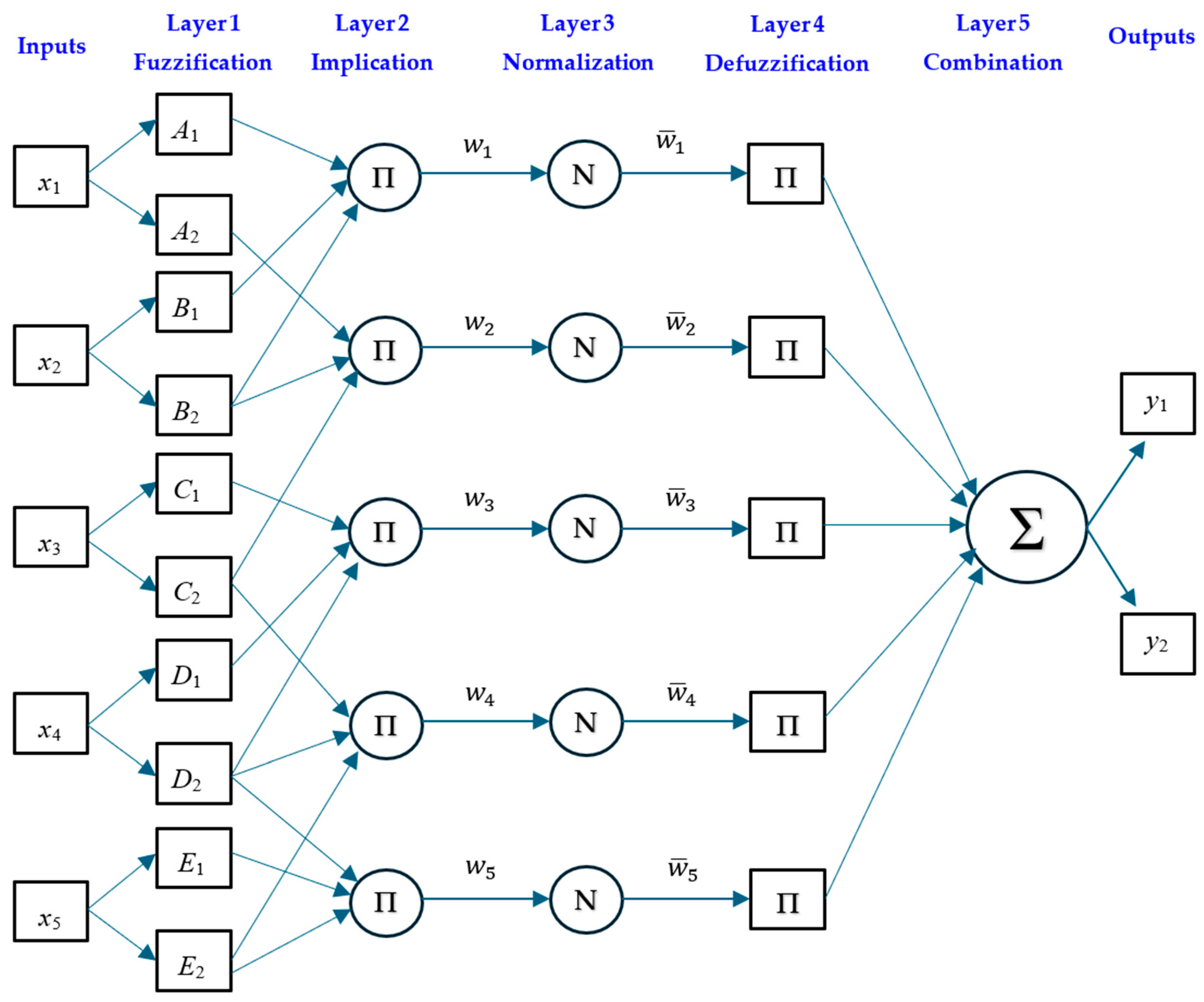
The structure of ANFIS and ANN models used in this study are illustrated in Figure 2 and Figure 3. As can be seen, the models have five inputs, namely initial concentrations of PZ, CO2 loading, temperature (°C), duration of thermal degradation test, and initial concentration of tertiary amines. The outputs of the model are the remaining concentrations of PZ and tertiary amines. As can be seen in Figure 2, the inputs of the model are inserted in the input layer. The ANN has one hidden layer and there are two outputs, namely the remaining PZ and tertiary amines. As can be seen in Figure 3, the ANFIS model has a more complex structure and layers, and in addition to input and output layers, there are layers such as fuzzification, implication, normalisation, defuzzification, and combination.
Artificial Neural Network (ANN)
Nonlinear computational models, such as ANNs, are widely used to address various engineering challenges [31]. In experimental predictions, ANNs have become the preferred approach, often outperforming traditional methods due to their ability to handle complex, nonlinear relationships. ANNs typically consist of three layers: an input layer, a hidden layer, and an output layer, where the number of neurons in the input and output layers corresponds to the respective input and output parameters. These networks rely on weighted connections between processing elements, with each neuron receiving inputs through weighted links. The output of a neuron can be expressed mathematically as
y = f i = 1 n ω i x i + b
where y is the output, f is the activation function, ω i are the weights, x i are the inputs, b is the bias, and n is the number of inputs. During training, the network adjusts these weights and biases using a suitable learning algorithm to minimise the root mean square error. A common approach is the gradient descent method [32].
Adaptive Neuro-Fuzzy Inference System (ANFIS)
The Adaptive Neuro-Fuzzy Inference System (ANFIS) is a hybrid intelligent model that combines the learning capabilities of neural networks with the reasoning power of fuzzy logic. It employs a five-layer architecture to map input–output relationships effectively. The ANFIS model can be mathematically represented using a set of if–then rules. For a system with five inputs ( x 1 , x 2 , x 3 , x 4 , x 5 ) and two outputs (z1, z2) (like this study), the general equation for the ANFIS model can be expressed as
Rule i if x 1 is A 1 i and x 2 is A 2 i and x 3 is A 3 i and x 4 is A 4 i and x 5 is A 5 i then
z 1 i = p 1 i x 1 + p 2 i x 2 + p 3 i x 3 + p 4 i x 4 + p 5 i x 5 + r 1 i z 2 i = q 1 i x 1 + q 2 i x 2 + q 3 i x 3 + q 4 i x 4 + q 5 i x 5 + r 2 i
A 1 i , A 2 i ,… are fuzzy sets for the five inputs. p 1 i ,… and q 1 i ,… and r 1 i and r 2 i are consequent parameters determined during the training process. i represents the rule number. The final outputs are calculated as weighted sums of the individual rule outputs:
z 1 = i = 1 n ω i z 1 i i = 1 n ω i
z 2 = i = 1 n ω i z 2 i i = 1 n ω i
where ω i represents the firing strength of each rule, and n is the total number of rules in the system [33]. Specifications of ANN and ANFIS models developed in this study are presented in Table 2.

2.2.2. Oxidative Degradation Models

For oxidative degradation, there were 14 inputs to the machine learning models, with the output being the remaining PZ concentration. Included in the inputs were the duration of the oxidative test (h), PZ type, partial pressures of CO2, O2, and N2, temperature, concentrations of K2SO4, Fe2+, Ni2+, Cr3+, Cu2+, and V4+, as well as Formate and Inhibitor.
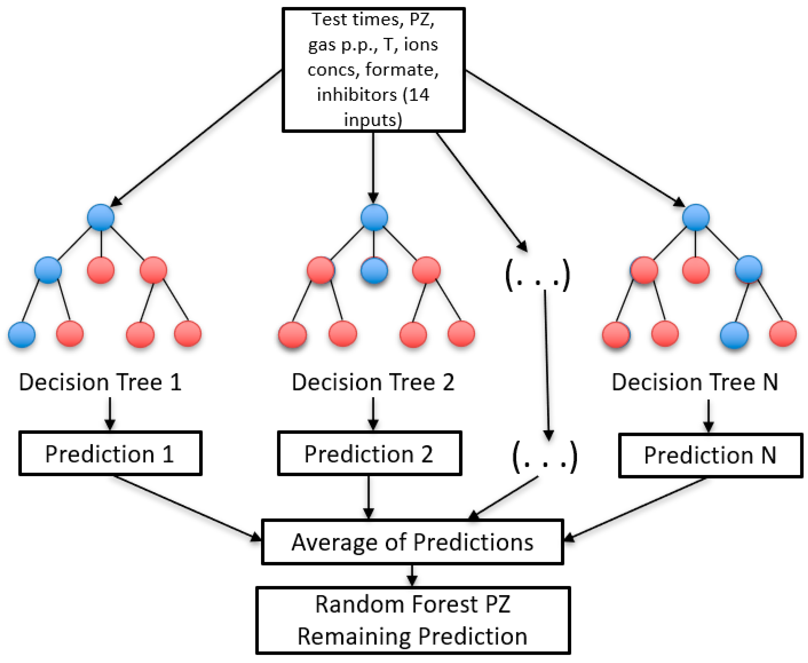
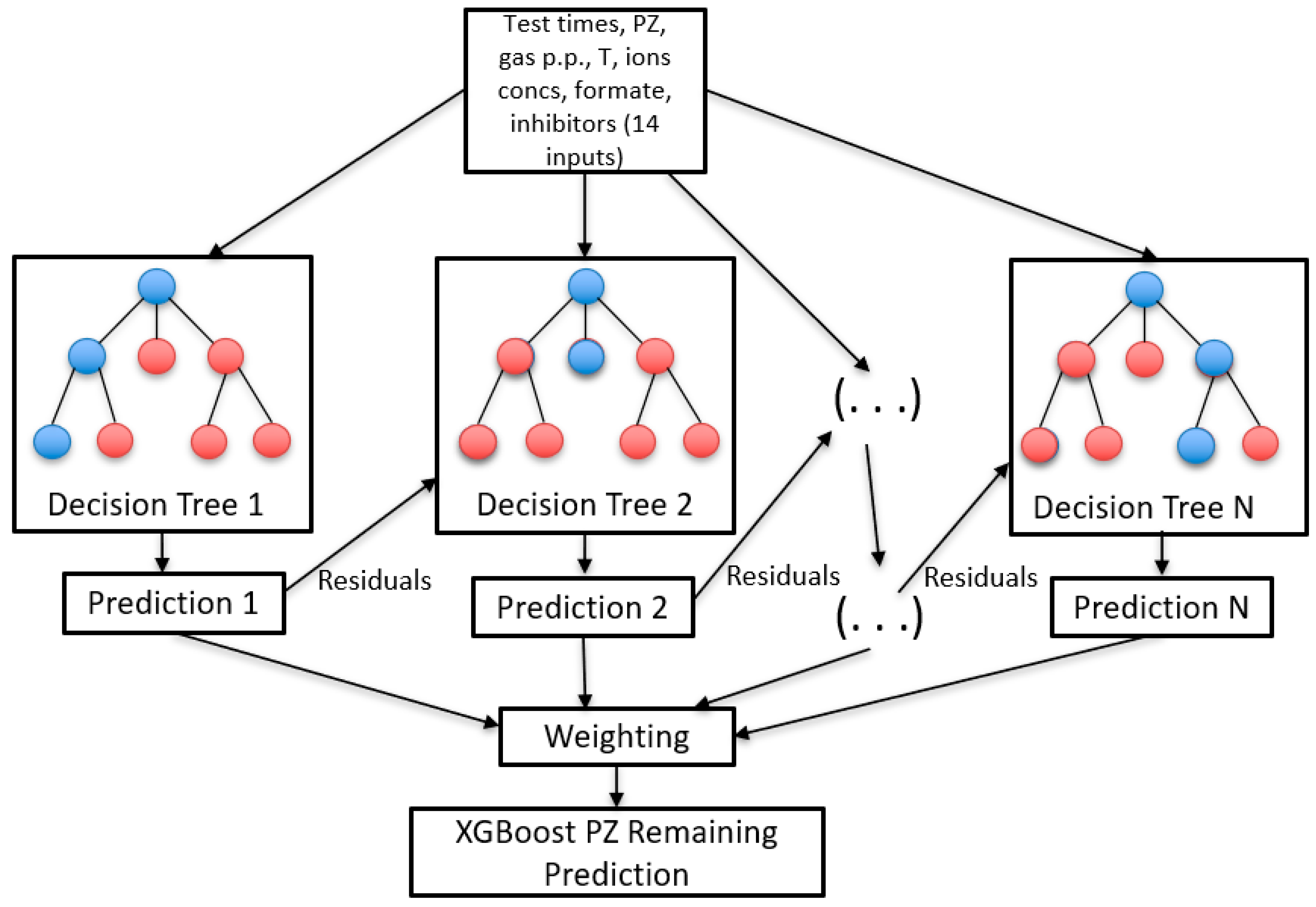
ANFIS and ANN models performed less well in the case of oxidative degradation, and a different approach was required. In addition to these, we tested Gaussian Processes (GP), Support Vector Machines (SVM), RFR, and XGBoost, all written in Python 3.13.7 using scikit-learn and Optuna 4.4.0 for hyperparameter optimisation. We performed 5-fold cross-validation to understand the generalisability of the models. While all models performed well on testing, only RFR and XGBoost performed sufficiently well after cross-validation and hence these models are discussed in more detail. The structure of RFR and XGBoost models used in this study are illustrated in Figure 4 and Figure 5.
Random Forest Regression (RFR)
RFR is an ensemble learning technique that has seen wide application for regression and classification. It works through generating multiple decision trees using bootstrap samples and then outputting the average prediction for regression applications [34]. This ensemble approach introduces randomness and decorrelation across trees, boosting performance and reducing overfitting. Mathematically, the RFR estimator is
f ^ x = 1 B b = 1 B f b ( x )
where B is the number of trees and f b x is the prediction from tree b . In engineering applications, RFR models have been applied to a variety of tasks like fault diagnosis and optimisation of energy systems. In the context of carbon capture, RFR models have seen good performance for predicting CO2 adsorption capacities of novel materials, such as metal–organic frameworks (MOFs) [35,36], and for optimising process parameters in capture technologies, including temperature swing adsorption [37]. RFR models’ ability to handle nonlinear relationships and rank feature importance makes them ideal for tackling the complexity of carbon capture systems.
XGBoost
Extreme Gradient Boosting (XGBoost) is a scalable, regularised boosting algorithm that has become known for its performance on structured data tasks, such as the one in this paper. It builds an ensemble of decision trees sequentially, rather than in parallel like with RF, each correcting the errors of its predecessors by minimising a differentiable loss function through gradient descent [38]. The model prediction after t iterations is
y i t ^ = k = 1 t f k x i , f k F
where F is the space of regression trees and each f k is a tree added at iteration k. The objective function is
L t = i l y i , y i t 1 ^ + f t x i + Ω f t
with Ω f = γ T + 1 2 λ | w | 2 serving as a regularisation term for tree complexity. XGBoost has seen wide use for applications in carbon capture, including prediction of CO2 solubility in ionic liquids [39] and MOFs [40]. Its ability to handle sparse inputs, quantify feature importance, and prevent overfitting with regularisation makes it a good algorithm for these applications. In our approach for these models, we use the Bayesian optimisation solver, Optuna, for hyperparameter optimisation [41,42]. Specifications of the optimised RF and XGBoost models developed in this study are presented in Table 3.

2.3. Model Performance Evaluation

In order to validate the machine learning models developed in the study, the determination coefficients ( R 2 ), the cross-validation coefficient ( Q 2 ), the root mean square error (RMSE), and the percentage average absolute relative error ( A A R E % ) are considered.
RMSE = i = 1 n D i e x p D i p r e d 2 n ;
AARE % = 100 i = 1 n D i e x p D i p r e d D i e x p n
R 2 = 1 i = 1 n D i e x p D i p r e d 2 i = 1 n D i e x p D ¯ 2
where D i e x p is the experimental amount of amine degradation, D i p r e d is the predicted amount of amine degradation, and D ¯ is the average amount of amine degradation. It should be noted that, as there are two outputs in this study, RMSE, AARE%, and R2 are calculated for each output separately for all train, validation, and test sets. In this study, model performance was considered acceptable when the coefficient of determination (R2) was near to 0.90, and the AARE below 5% was considered an excellent model, AARE% between 5 and 10% a good model, and between 10 and 20% was acceptable, considering the complexity of amine degradation chemistry and the variability of experimental conditions reported in the literature, in line with commonly used thresholds in the literature. Values of R2 above 0.95 and AARE below 5% were regarded as very good indicators of predictive accuracy. R2 reflects the overall correlation and goodness of fit, RMSE penalises large errors and reflects the absolute predictive accuracy, and AARE% normalises the error relative to the magnitude of the experimental values, which is important given the wide range of degradation data. By using these three metrics together, we ensured a more reliable and holistic evaluation of the models, avoiding bias that might arise from relying on a single metric. For the oxidative degradation models, 5-fold cross-validation was employed to evaluate the model performance by calculating the mean absolute error (MAE) and its standard deviation across the folds.

3. Results and Discussion

In this section, the results of each model are presented, and the performance of each model is discussed. The results of the ANN and ANFIS models for thermal degradation are presented in Table 4 and Table 5, with the results for the RF and XGBoost models for oxidative degradation are presented in Table 6.

3.1. Thermal Degradation Results

3.1.1. ANN Model Results

As mentioned, the model aims to estimate the remaining concentrations of both PZ (Output 1) and the tertiary amine (Output 2) after thermal degradation. As can be seen in Table 4, the ANN model demonstrates good predictive performance across all PZ-tertiary amine mixtures. The R2 values for Output 1 and Output 2 remain consistently high across all datasets, with PZ-DMAP showing the most accurate predictions (R2 > 0.99 in all cases). For example, in the test set, PZ-DMAP achieves R2 values of 0.9949 (Output 1) and 0.9960 (Output 2), confirming its outstanding model fit and generalisation capability. Similarly, PZ-DMAE and PZ-DEAE also yield strong performances, with test R2 values greater than 0.96 for both outputs. In contrast, the PZ-TEA mixture exhibits slightly lower R2 values, particularly for Output 2 (e.g., 0.9272 in the test set), indicating a moderately reduced predictive performance compared to other systems. Nevertheless, the model still maintains acceptable levels of accuracy, suggesting it remains a viable tool even for mixtures with more complex degradation behaviour.
The RMSE values provide further confirmation of the ANN model’s reliability. The lowest RMSE values are observed for the PZ-DMAP system, with test RMSEs of 0.0438 (Output 1) and 0.0415 (Output 2), signifying minimal deviation between predicted and actual values. In contrast, PZ-DEAE and PZ-TEA exhibit slightly elevated RMSE values for Output 2 (e.g., 0.0977 and 0.1774, respectively), which is consistent with their lower R2 scores. The AARE% metric corroborates these findings. PZ-DMAP again performs the best, with AARE% values as low as 1.21% (Output 1) and 2.58% (Output 2) on the test data, indicating extremely accurate predictions. Conversely, PZ-TEA and PZ-DMAE show higher AARE% values, especially for Output 2, with values reaching up to 11.63%, suggesting that the thermal degradation profile for these mixtures may be more nonlinear or complex, requiring further model tuning or input features for improved prediction.
These findings demonstrate the ANN model’s strong generalizability and highlight its potential as a predictive tool for evaluating thermal degradation in amine-based CO2 capture systems. The use of machine learning models in this context not only reduces the need for extensive experimental trials but also offers insights into which solvent combinations are most stable under thermal degradation.
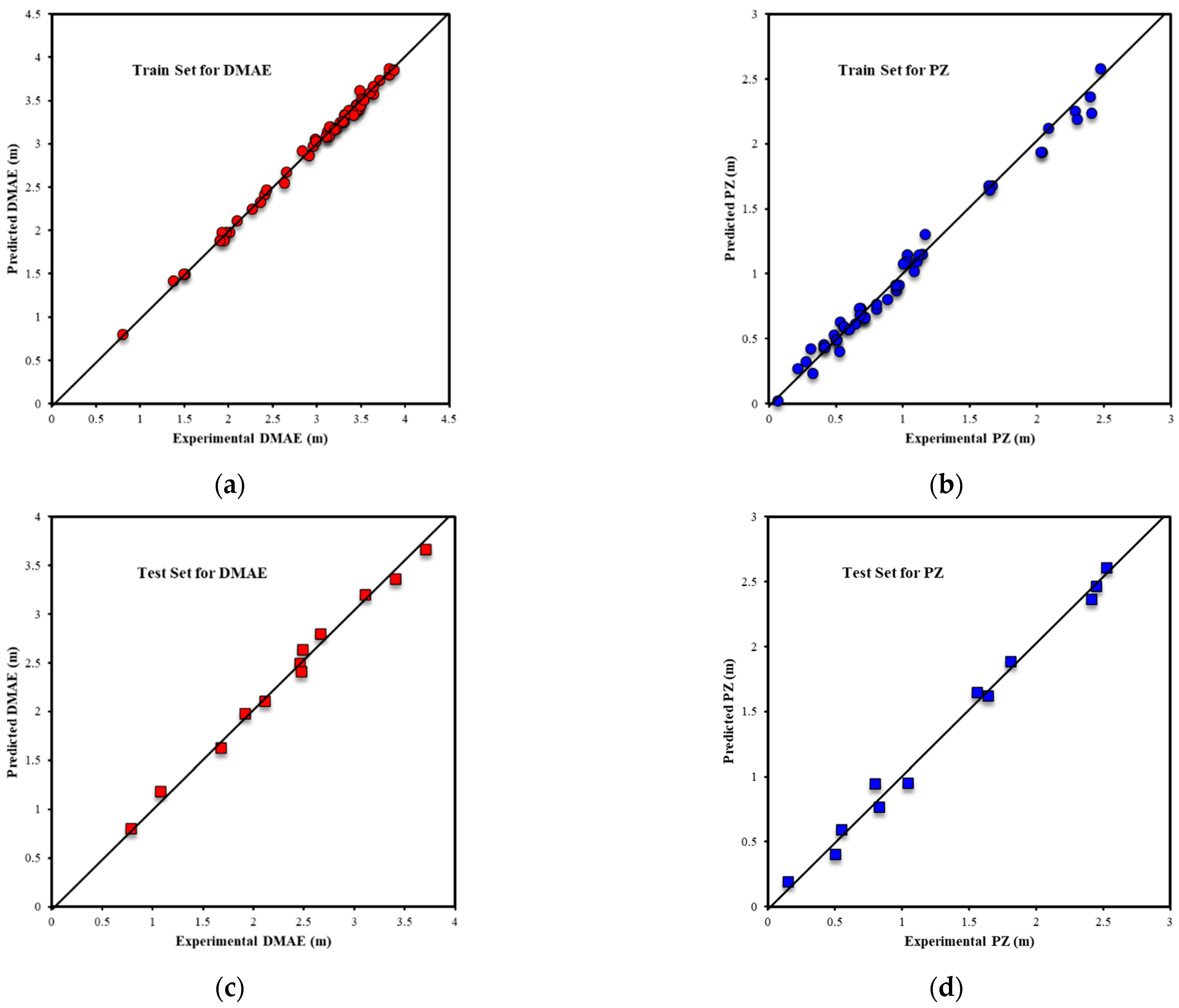
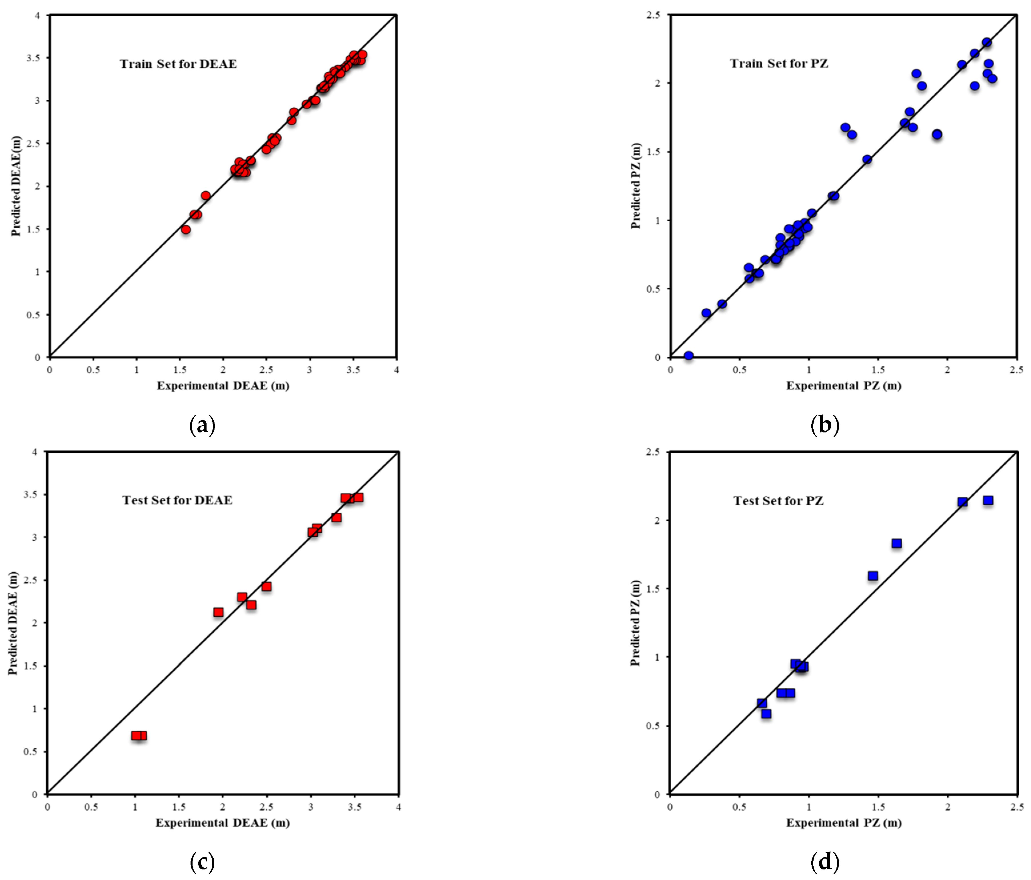
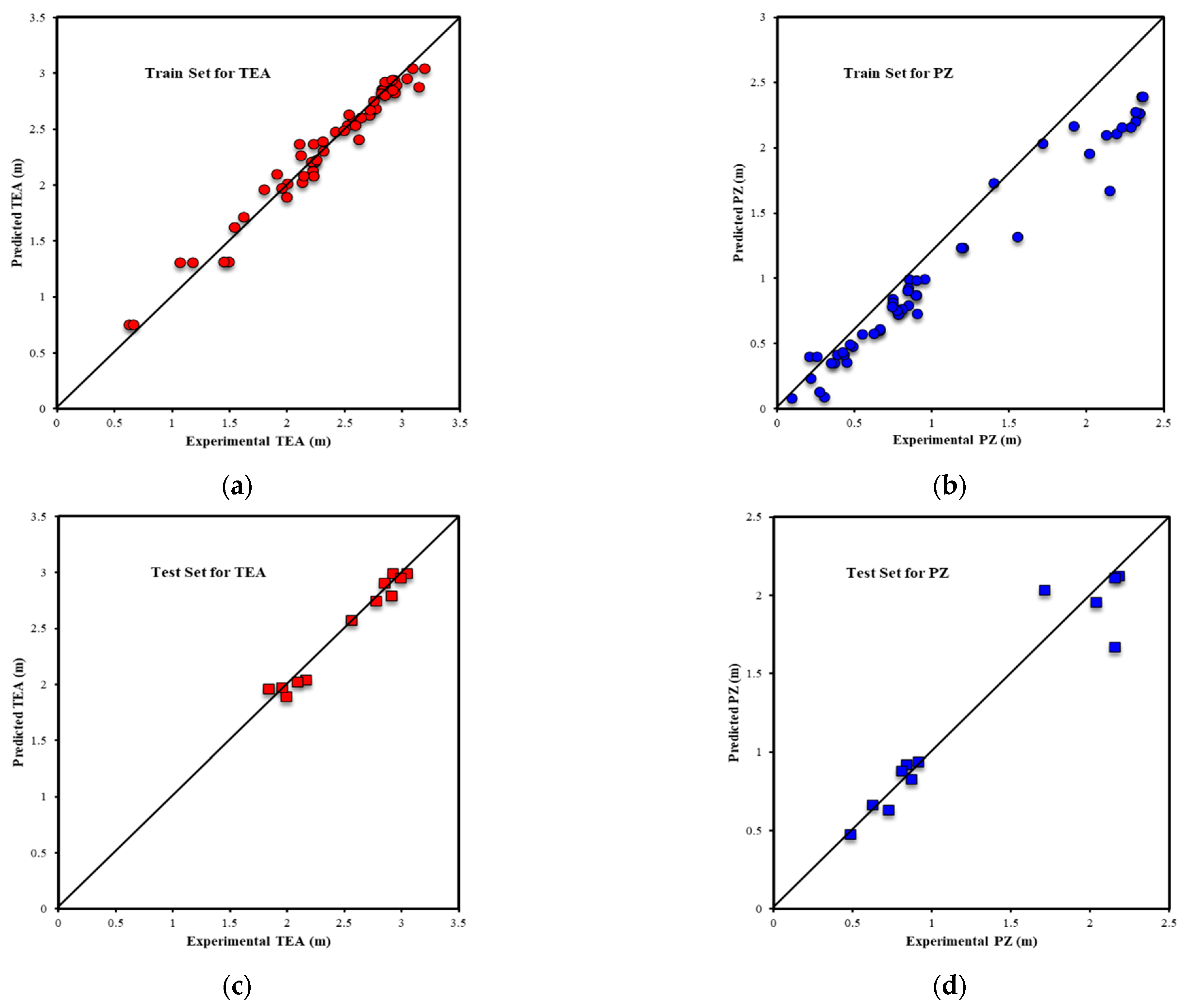
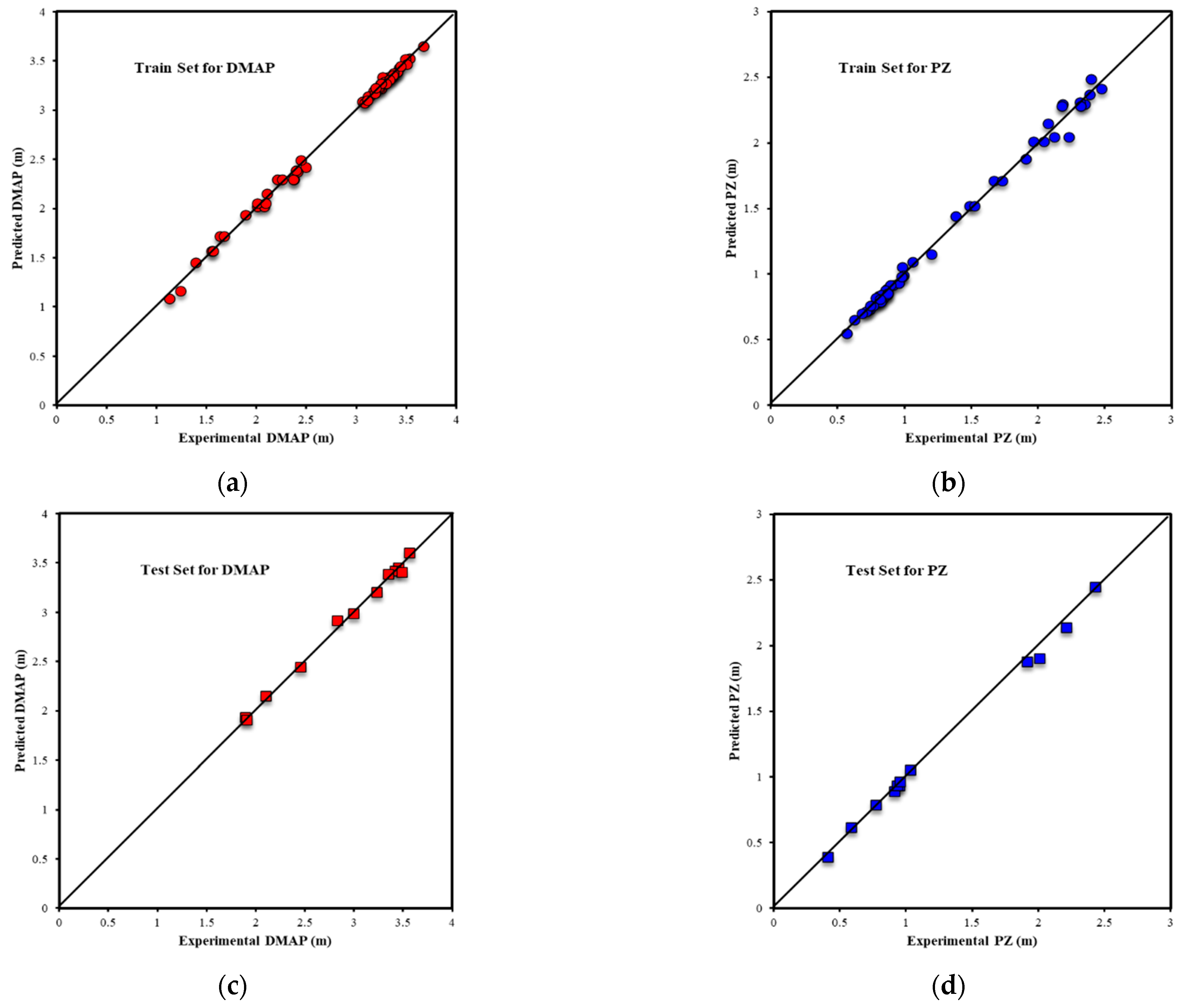
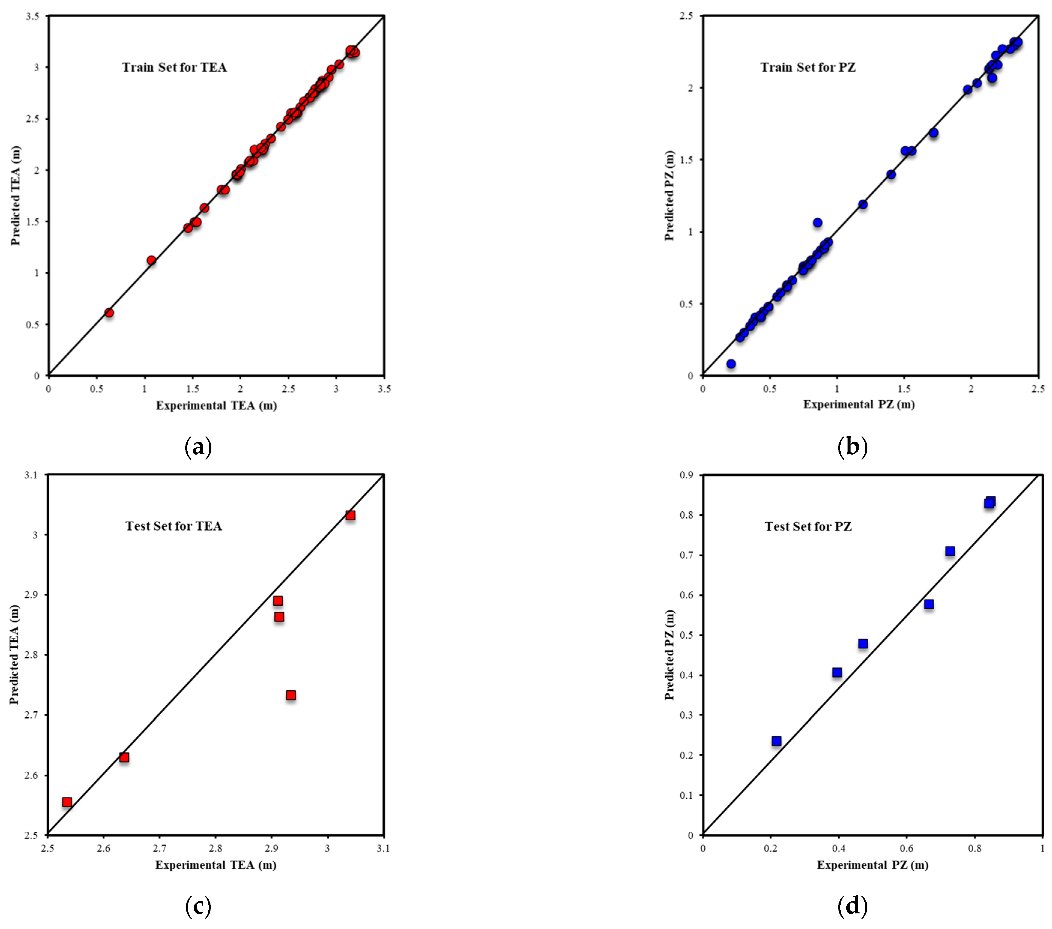
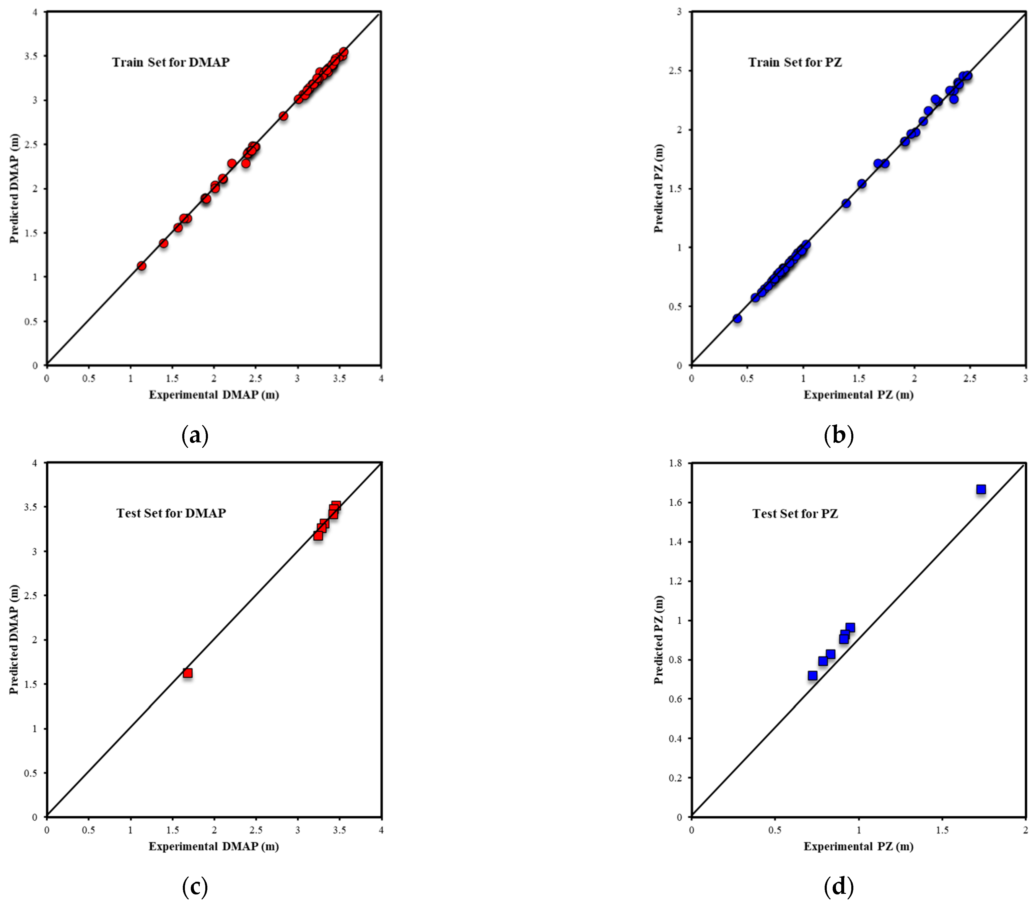
Figure 6, Figure 7, Figure 8, Figure 9 and Figure 10 illustrate the performance of artificial neural network (ANN) models developed to predict the degradation behaviour of various amine–PZ solvent mixtures. Each figure corresponds to a specific amine combined with PZ and highlights the model’s predictive accuracy by comparing experimental values against ANN-predicted outputs.
Each figure contains model performance plots as parity plots showing how well the ANN model captures the complex nonlinear degradation behaviour of the mixture under various conditions. Across all mixtures, the plots demonstrate a strong correlation between predicted and experimental values. This is evident from the tight clustering of points along the ideal 45-degree line (y = x), suggesting that the ANN models are well-trained and generalise effectively for the datasets used. While the amines differ in chemical structure and degradation potential, the ANN models show comparable levels of performance for each mixture. This indicates the flexibility of the ANN approach in modelling solvent degradation dynamics, regardless of the specific amine used. These results validate the utility of ANN models as reliable tools for predicting solvent degradation, which is a critical parameter in carbon capture applications. The ability to forecast degradation behaviour can significantly reduce the need for extensive experimental campaigns and support early-stage screening of novel solvent systems. The strong performance also reflects the quality of the input data used for training, as well as appropriate model architecture and parameter tuning. This suggests that the ANN was well designed to accommodate the variability in degradation behaviour introduced by different amine functional groups.

3.1.2. ANFIS Model Results

Similar to the ANN model, the ANFIS model also aimed to estimate the remaining concentrations of both PZ (Output 1) and the tertiary amine (Output 2) after thermal degradation. As can be seen in Table 5, the ANFIS model demonstrates high overall predictive accuracy for most amine mixtures, particularly for PZ-DMAP, which consistently yielded the best results across all metrics. On the test set, PZ-DMAP achieves R2 values of 0.9330 (Output 1) and 0.9852 (Output 2), with exceptionally low RMSE and AARE% values, indicating strong generalisation and minimal prediction error. Similarly, PZ-DEAE and PZ-MDEA also show competitive performance, especially in training and validation phases.
For PZ-MDEA, the model achieves R2 values above 0.96 for all data subsets and outputs, with low RMSE (e.g., 0.0208 and 0.0173 for test set) and AARE% as low as 0.66% and 2.88%, indicating a robust fit. The PZ-TEA system shows strong overall and training performance but has a relatively lower R2 in the test set for Output 1 (0.8913), suggesting slightly reduced generalisation for predicting the remaining amount of PZ. In contrast, the PZ-DMAE mixture exhibited a significant drop in predictive accuracy for Output 1 in the test phase (R2 = 0.7211, RMSE = 0.2145, AARE% = 5.20%), indicating more complex degradation behaviour or greater data variability that the ANFIS model struggled to capture. However, Output 2 remains well predicted (R2 = 0.9785), pointing to asymmetry in model performance for different chemical components. The validation set performance across all systems was generally strong but shows notable fluctuations, particularly for PZ-MDEA and PZ-DEAE, where Output 2 validation R2 drops below 0.90. This suggests potential overfitting in training or a need for improved fuzzification/clustering strategies during model development. Nevertheless, PZ-DMAP again shows reliable behaviour, with validation and test R2 consistently above 0.98, highlighting its suitability for predictive modelling using ANFIS.
The relatively lower predictive accuracy observed for PZ–TEA compared to PZ–DMAP can be explained by their underlying chemical behaviour. Tertiary amines such as TEA follow multiple competing oxidative and thermal degradation pathways, often producing diverse by-products, which results in more nonlinear behaviour and greater variability in the data. By contrast, DMAP exhibits higher structural stability under the studied conditions, which is consistent with the stronger model performance and lower experimental scatter observed for PZ–DMAP.
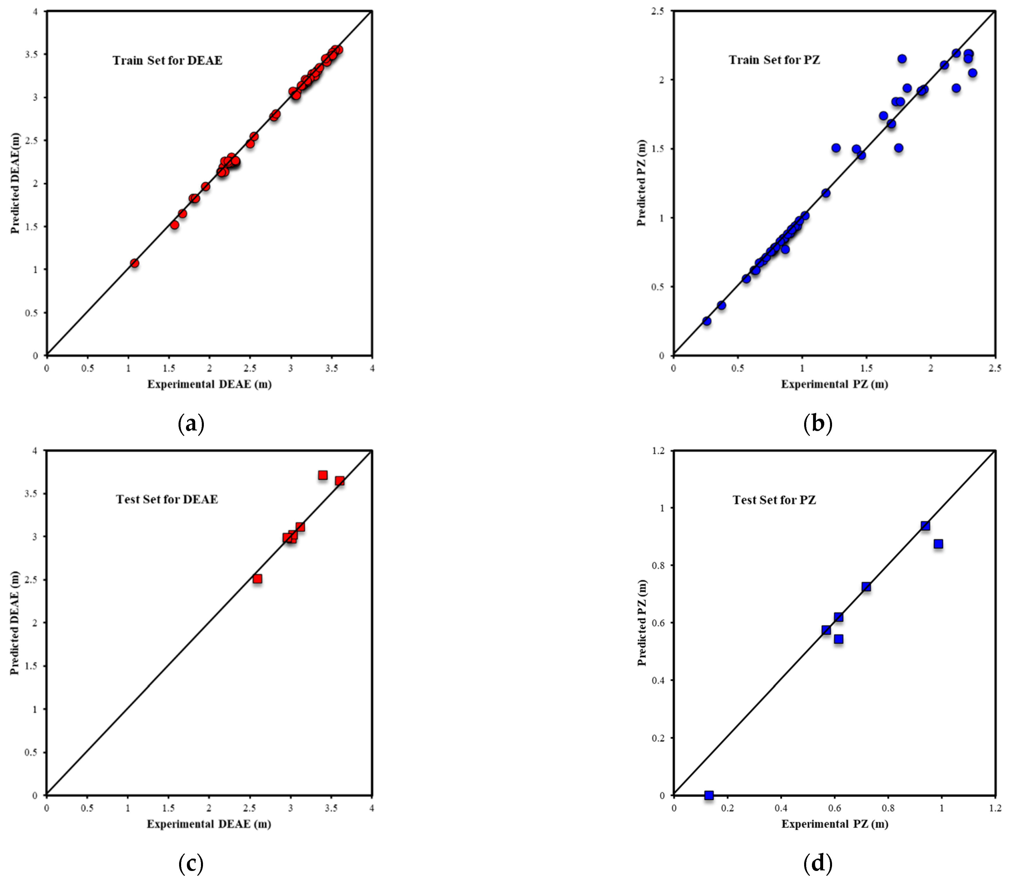
When compared to the ANN model, ANFIS showed comparable or slightly better performance for certain amine systems such as PZ-MDEA and PZ-DMAP, especially for Output 2 predictions. However, in systems with more nonlinear behaviour like PZ-DMAE, ANN outperformed ANFIS in predictive accuracy for Output 1. This reinforces the idea that while ANFIS models can capture fuzzy rules and nonlinear interactions effectively, they may be more sensitive to noise or limited data in high-variance systems. Similar to the ANN model, predicted vs. experimental graphs are illustrated in Figure 11, Figure 12, Figure 13, Figure 14 and Figure 15. The plots demonstrate a strong agreement between predicted and experimental degradation values, indicating the ANFIS models’ high accuracy and effectiveness. These results highlight the suitability of ANFIS in modelling complex nonlinear degradation behaviours in solvent systems used for CO2 capture, providing a reliable predictive tool for evaluating solvent stability. In some cases, the AARE reached values around 20%. Given the complexity of amine degradation chemistry and the variability of experimental conditions reported in the literature, this level of error is considered acceptable.

3.2. Oxidative Degradation Results

As mentioned in Section 2.2.2, in addition to thermal degradation, oxidative degradation is also considered in this study. To model the oxidative degradation of PZ, two ensemble-based machine learning approaches, RFR and XGBoost, are implemented. The choice of these models was motivated by lower performance from neural network architectures for these datasets. Both models utilised 14 input features related to experimental conditions, including test duration, PZ type, gas partial pressures (CO2, O2, N2), temperature, concentrations of K2SO4, Fe2+, Ni2+, Cr3+, Cu2+, and V4+, formate, and inhibitor presence. The target output was the remaining concentration of PZ after the oxidative degradation experiment. In both RFR and XGBoost models, 70% of the data was used for train, 15% for validation, and 15% for test.
As can be seen in Table 6, both models demonstrated strong predictive capabilities across training, validation, and test datasets. The RF model achieved slightly higher R2 on the training set (0.9722), indicating an excellent model fit. However, the XGBoost model outperformed RF on the test set, with an R2 of 0.8900 compared to 0.8655 for RF. This suggests that XGBoost may generalise slightly better on unseen data, despite having a less training fit. Similarly, in terms of RMSE, RF exhibited a lower training error (0.0997 vs. 0.1354 for XGBoost), but XGBoost achieved lower RMSE values on the validation and test sets (0.2230 and 0.2085, respectively), implying a more stable and generalizable model across experimental conditions.
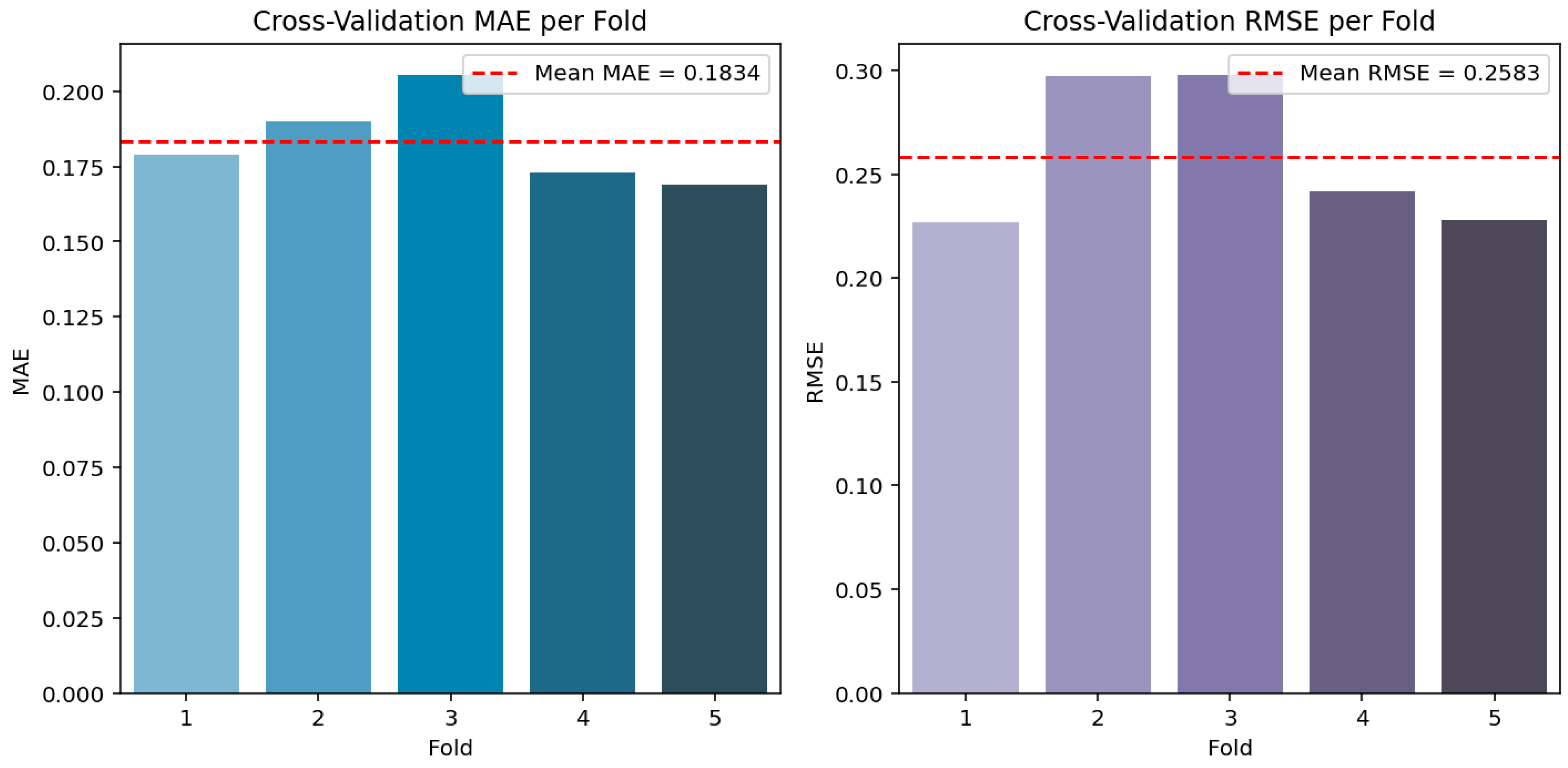
The Average Absolute Relative Error (AARE%) also confirms this trend. While RF performs better in training (1.65% vs. 2.61%), XGBoost yielded lower AARE values in both the validation (5.15% vs. 5.35%) and test (3.97% vs. 3.90%) datasets, albeit with very close margins. To further evaluate robustness, a 5-fold cross-validation was applied. The mean MAE for RF was slightly lower (0.1735 vs. 0.1834), but XGBoost showed a smaller standard deviation (0.0132 vs. 0.0208), suggesting better consistency across folds and potentially greater stability in practical applications.
RF offers a strong fit and slightly better average error performance on training data, while XGBoost provides better generalisation to unseen data, especially under diverse experimental setups. This is crucial for practical deployment, where robustness and adaptability across varying degradation scenarios are required. Note that since both models are cross-validated and hyperparameters are optimised rigorously in all cases, these results are not the result of chance data selection during fitting, but we can conclude that RFR may tend to slightly overfitting more than XGBoost, and that XGBoost has better generalisability for these problems.

3.2.1. Random Forest Results

Figure 16 presents the predictive performance of the RF model for the oxidative degradation of PZ by comparing the predicted concentrations of PZ with their corresponding experimental values. The results are shown separately for the training (left) and test (right) datasets. As observed in the left panel, the RF model exhibits good agreement between predicted and experimental values for the training set. The data points closely follow the 45-degree line, indicating high predictive accuracy. This observation aligns with the statistical metrics presented previously, which confirm that the model effectively captures the underlying relationships between the input features and the oxidative degradation behaviour of PZ during training.
In the right panel, representing the test dataset, the RF model maintains a reasonably good prediction capability, though the scatter around the 1:1 line slightly increases. This is expected due to the inherent variability in test data and the model’s exposure to unseen samples. The test performance remains strong, indicating that the model generalises well and is capable of estimating PZ degradation under varying experimental conditions. The slight under- or over-estimation seen in a few data points could be attributed to the complexity of oxidative degradation pathways and potential noise in the experimental measurements. Nevertheless, the RF model demonstrates reliable performance in predicting residual PZ concentrations, supporting its applicability for modelling degradation behaviour in real systems.
Figure 17 illustrates the feature importance values derived from the RF model used to predict the oxidative degradation of the PZ solution. The most influential variables identified by the model are the duration of the oxidative test (Dur), oxygen partial pressure (O2 kPa), and carbon dioxide partial pressure (CO2 kPa), indicating their dominant roles in governing the extent of PZ degradation. Other relevant contributors include copper ion concentration (Cu2+), inhibitor concentration, and temperature. Conversely, variables such as vanadium (V4+), nitrogen pressure (N2 kPa), and formate showed minimal influence. These insights are critical for prioritising process parameters in efforts to minimise oxidative degradation and extend the operational lifetime of amine solvents in industrial applications.
Figure 18 presents the cross-validation performance metrics of the RF model for predicting oxidative degradation of PZ, showing both Mean Absolute Error (MAE) and Root Mean Square Error (RMSE) across five folds. The average MAE across all folds was 0.1735, with the lowest error observed in Fold 5. Similarly, the RMSE averaged at 0.2591, with a gradual decrease from Fold 1 to Fold 5, indicating improved predictive consistency in later folds. The relatively low variation across folds highlights the robustness and generalisation capability of the RF model in modelling the complex relationships influencing PZ degradation.

3.2.2. XGBoost Results

Figure 19 illustrates the predictive performance of the XGBoost model in estimating oxidative degradation of PZ based on experimental data. The left panel shows the correlation between predicted and experimental values for the training set, demonstrating a strong agreement with minimal dispersion around the diagonal line. The test set results, shown in the right panel, similarly display a tight clustering of predicted values around the diagonal, indicating that the model generalises well to unseen data. Overall, the XGBoost model demonstrates high predictive accuracy and robustness in capturing the nonlinear relationships influencing PZ degradation.
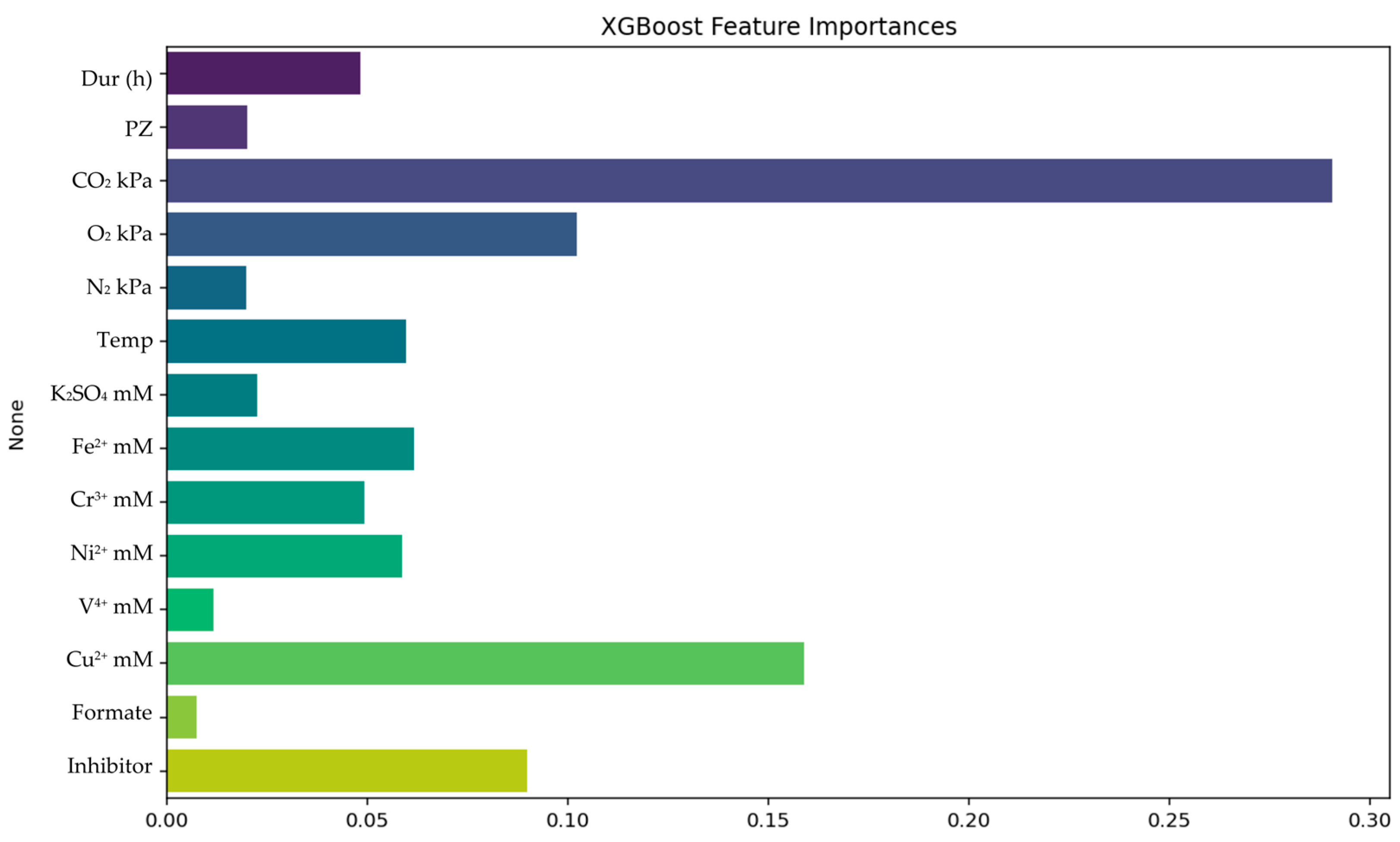
Figure 20 presents the results of a feature importance analysis for the input parameters used in the XGBoost model. The bar plot ranks the features based on their relative importance in influencing the model’s predictions. Among all the variables, carbon dioxide partial pressure stands out as the most significant feature, indicating that it has the greatest impact on the model’s output. This is followed by copper ion concentration, inhibitor concentration, and oxygen partial pressure, which also contribute notably to the predictive power of the model. In contrast, features such as vanadium (V4+), nitrogen pressure (N2 kPa), and formate showed considerably lower importance, suggesting that they play a minor role in the model’s decision-making process, which is similar to the RF model results. Understanding these features helps to identify which parameters are most influential, guiding experimental focus and further model optimisation.
Figure 21 displays the results of 5-fold cross-validation for the XGBoost model, evaluating both MAE and RMSE across the folds. The left panel shows the MAE values for each fold, with a mean MAE of 0.1834 (indicated by the dashed red line). The variability between folds is relatively low, suggesting consistent model performance in terms of absolute error. The right panel presents the RMSE values per fold, with a mean RMSE of 0.2583. The RMSE plot reveals slightly larger variation across the folds compared to the MAE, particularly in folds 2 and 3, which have higher error values. Overall, the cross-validation results indicate that the XGBoost model achieves stable and reliable prediction accuracy, as evidenced by the narrow range of error metrics across the validation splits.

4. Conclusions

This study examines the thermal degradation of piperazine mixed with five tertiary amines—PZ-MDEA, PZ-TEA, PZ-DMAE, PZ-DEAE, and PZ-DMAP—under varying CO2 loadings, temperatures, absorption durations, and amine solution concentrations. For each mixture, 77 data points were selected. Then, in general, 385 data points were used in this study. Artificial Neural Network (ANN) and Adaptive Neuro-Fuzzy Inference System (ANFIS) models were trained, validated, and tested using the coefficient of determination (R2), root mean square error (RMSE), and average absolute relative error (AARE). Both models demonstrated strong predictive capabilities for amine degradation with high statistical performance. In addition to thermal degradation, oxidative degradation of the PZ solution is also considered in this study using Random Forest (RF) and Extreme Gradient Boosting (XGBoost) models using more than 200 data points. The same statistical parameters are used to validate the models. In addition, feature importance test and cross-validation are performed. This methodology enables rapid prediction of amine degradation and can be integrated into process models and increase the sustainability of the CO2 absorption process. It must be mentioned that having more data points for each amine mixture can result in more reliable models. Hence, more experimental data is needed for the prediction of amine degradations.

Supplementary Materials

The following supporting information can be downloaded at https://www.mdpi.com/article/10.3390/su172210311/s1, Thermal degradation and oxidative degradation data.

Author Contributions

Conceptualization, T.N.B.; methodology, T.N.B. and M.S.; software, T.N.B. and M.S.; validation, T.N.B. and M.S.; formal analysis, T.N.B.; investigation, T.N.B.; data curation, T.N.B.; writing—original draft preparation, T.N.B. and M.S.; writing—review and editing, T.N.B.; visualization, T.N.B. and M.S.; supervision, T.N.B.; project administration, T.N.B. All authors have read and agreed to the published version of the manuscript.

Funding

This research received no external funding.

Institutional Review Board Statement

Not applicable.

Informed Consent Statement

Not applicable.

Data Availability Statement

The raw data supporting the conclusions of this article are available in Supplementary Materials.

Conflicts of Interest

The authors declare no conflict of interest.

References

  1. Elmarghni, S.; Ansarpour, M.; Borhani, T.N. Effect of Different Amine Solutions on Performance of Post-Combustion CO2 Capture. Processes 2025, 13, 2521. [Google Scholar] [CrossRef]
  2. Gouedard, C.; Picq, D.; Launay, F.; Carrette, P.L. Amine degradation in CO2 capture. I. A review. Int. J. Greenh. Gas Control 2012, 10, 244–270. [Google Scholar] [CrossRef]
  3. Namjoshi, O.A. Thermal Degradation of PZ-Promoted Tertiary Amines for CO2 Capture. Ph.D. Thesis, The University of Texas at Austin, Austin, TX, USA, 2015. [Google Scholar]
  4. Thompson, J.G.; Gao, X.; Toma, S.; Abad, K.; Bhatnagar, S.; Landon, J.; Liu, K. Decomposition of N-nitrosamines formed in CO2 capture systems through electrochemically-mediated reduction on carbon xerogel electrode. Int. J. Greenh. Gas Control 2019, 83, 83–90. [Google Scholar] [CrossRef]
  5. Hatchell, D.; Namjoshi, O.; Fischer, K.; Rochelle, G.T. Thermal Degradation of Linear Amines for CO2 Capture. Energy Procedia 2014, 63, 1558–1568. [Google Scholar] [CrossRef]
  6. Vega, F.; Sanna, A.; Navarrete, B.; Maroto-Valer, M.M.; Cortés, V.J. Degradation of amine-based solvents in CO2 capture process by chemical absorption. Greenh. Gases Sci. Technol. 2014, 4, 707–733. [Google Scholar] [CrossRef]
  7. Liu, H.; Namjoshi, O.A.; Rochelle, G.T. Oxidative Degradation of Amine Solvents for CO2 Capture. Energy Procedia 2014, 63, 1546–1557. [Google Scholar] [CrossRef]
  8. Peeters, W.; Neerup, R.; Fosbøl, P.L. Solvent degradation & influences on amine-based carbon capture operations. Int. J. Greenh. Gas Control 2025, 147, 104500. [Google Scholar] [CrossRef]
  9. Vevelstad, S.J.; Buvik, V.; Knuutila, H.K.; Grimstvedt, A.; da Silva, E.F. Important Aspects Regarding the Chemical Stability of Aqueous Amine Solvents for CO2 Capture. Ind. Eng. Chem. Res. 2022, 61, 15737–15753. [Google Scholar] [CrossRef]
  10. Borhani, T.N.; García-Muñoz, S.; Vanesa Luciani, C.; Galindo, A.; Adjiman, C.S. Hybrid QSPR models for the prediction of the free energy of solvation of organic solute/solvent pairs. Phys. Chem. Chem. Phys. 2019, 21, 13706–13720. [Google Scholar] [CrossRef] [PubMed]
  11. Martin, S.; Lepaumier, H.; Picq, D.; Kittel, J.; De Bruin, T.; Faraj, A.; Carrette, P.L. New Amines for CO2 Capture. IV. Degradation, Corrosion, and Quantitative Structure Property Relationship Model. Ind. Eng. Chem. Res. 2012, 51, 6283–6289. [Google Scholar] [CrossRef]
  12. Azarpour, A.; Zendehboudi, S. Hybrid Smart Strategies to Predict Amine Thermal Degradation in Industrial CO2 Capture Processes. ACS Omega 2023, 8, 26850–26870. [Google Scholar] [CrossRef]
  13. Davis, J.D. Thermal Degradation of Aqueous Amines used for Carbon Dioxide Capture. Ph.D. Thesis, The University of Texas at Austin, Austin, TX, USA, 2009. [Google Scholar]
  14. Kottala, R.K.; Chigilipalli, B.K.; Mukuloth, S.; Shanmugam, R.; Kantumuchu, V.C.; Ainapurapu, S.B.; Cheepu, M. Thermal Degradation Studies and Machine Learning Modelling of Nano-Enhanced Sugar Alcohol-Based Phase Change Materials for Medium Temperature Applications. Energies 2023, 16, 2187. [Google Scholar] [CrossRef]
  15. Muchan, P.; Supap, T.; Narku-Tetteh, J.; Lisawadi, S.; Idem, R. The relationship between oxidative degradation and ammonia emission of carbon capture amines based on their chemical structures. Clean Energy 2024, 8, 134–152. [Google Scholar] [CrossRef]
  16. Wagaarachchige, J.D.; Idris, Z.; Khatibzadeh, A.; Drageset, A.; Jens, K.J.; Halstensen, M. Demonstration of CO2 Capture Process Monitoring and Solvent Degradation Detection by Chemometrics at the Technology Centre Mongstad CO2 Capture Plant. Ind. Eng. Chem. Res. 2023, 62, 9747–9754. [Google Scholar] [CrossRef]
  17. Wagaarachchige, J.D.; Idris, Z.; Khatibzadeh, A.; Drageset, A.; Jens, K.J.; Halstensen, M. Demonstration of CO2 Capture Process Monitoring and Solvent Degradation Detection by Chemometrics at the Technology Centre Mongstad CO2 Capture Plant: Part II. Ind. Eng. Chem. Res. 2024, 63, 10704–10712. [Google Scholar] [CrossRef]
  18. Buvik, V.; Høisæter, K.K.; Vevelstad, S.J.; Knuutila, H.K. A review of degradation and emissions in post-combustion CO2 capture pilot plants. Int. J. Greenh. Gas Control 2021, 106, 103246. [Google Scholar] [CrossRef]
  19. Chen, P.; Wang, D.; Yi, N.; Jiang, J.; Herraiz, L.; Zhou, X.; Chen, J.; Ren, Y.; Xu, S.; Garcia, S.; et al. Amine-based carbon capture through an environmental lens: Amine emissions and associated implications. J. Environ. Chem. Eng. 2025, 13, 119605. [Google Scholar] [CrossRef]
  20. Muchan, P.; Kruthasoot, S.; Kongton, T.; Supap, T.; Narku-Tetteh, J.; Lisawadi, S.; Srisuradetchai, P.; Idem, R. Development of a Predictive Model to Correlate the Chemical Structure of Amines with Their Oxidative Degradation Rate in a Post-Combustion Amine-Based CO2 Capture Process Using Multiple Linear Regression and Machine Learning Regression Approaches. ACS Omega 2024, 9, 6669–6683. [Google Scholar] [CrossRef] [PubMed]
  21. Irvin, B.D.; Jones, T.; Pelgen, J.V.; Fan, Z.; Abad, K.; Bhatnagar, S.; Frimpong, R.A.; Nikolic, H.; Thompson, J.; Liu, K. Determining alkalinity, carbon loading, and degradation of aqueous amine in CO2 capture processes using heuristic methods. Int. J. Greenh. Gas Control 2025, 145, 104394. [Google Scholar] [CrossRef]
  22. Braakhuis, L.; Høisæter, K.K.; Knuutila, H.K. Modeling the Formation of Degradation Compounds during Thermal Degradation of MEA. Ind. Eng. Chem. Res. 2022, 61, 2867–2881. [Google Scholar] [CrossRef]
  23. Braakhuis, L.; Knuutila, H.K. Predicting solvent degradation in absorption–based CO2 capture from industrial flue gases. Chem. Eng. Sci. 2023, 279, 118940. [Google Scholar] [CrossRef]
  24. Dickinson, J.; Percy, A.; Puxty, G.; Verheyen, T.V. Oxidative degradation of amine absorbents in carbon capture systems—A dynamic modelling approach. Int. J. Greenh. Gas Control 2016, 53, 391–400. [Google Scholar] [CrossRef]
  25. Yoon, B.; Stowe, H.M.; Hwang, G.S. Molecular mechanisms for thermal degradation of CO2-loaded aqueous monoethanolamine solution: A first-principles study. Phys. Chem. Chem. Phys. 2019, 21, 22132–22139. [Google Scholar] [CrossRef]
  26. Parks, C.; Alborzi, E.; Akram, M.; Pourkashanian, M. DFT Studies on Thermal and Oxidative Degradation of Monoethanolamine. Ind. Eng. Chem. Res. 2020, 59, 15214–15225. [Google Scholar] [CrossRef]
  27. Parks, C.; Hughes, K.J.; Pourkashanian, M. Furthering the understanding of product formation in monoethanolamine degradation: A mechanistic DFT study. Int. J. Greenh. Gas Control 2022, 119, 103732. [Google Scholar] [CrossRef]
  28. Yu, J.; Patel, D.; Hwang, G.S. First-Principles Prediction of the Critical Role of Superoxide Anions in Oxidative Degradation of Aqueous Amine Solvents for Carbon Dioxide Capture. Ind. Eng. Chem. Res. 2025, 64. [Google Scholar] [CrossRef]
  29. He, Z.; He, L.; Wang, L.; Wang, W.; Ma, D.; Yao, Q.; Sun, M. Thermal oxidation degradation mechanism under the rust-catalyzed condition of CO2 absorbent monoethanolamine and the DFT analysis of pathway. J. Environ. Chem. Eng. 2025, 13, 116189. [Google Scholar] [CrossRef]
  30. Freeman, S.A. Thermal Degradation and Oxidation of Aqueous Piperazine for Carbon Dioxide Capture. Ph.D. Thesis, The University of Texas at Austin, Austin, TX, USA, 2011. [Google Scholar]
  31. Yan, Y.; Borhani, T.N.; Clough, P.T. Chapter 14: Machine Learning Applications in Chemical Engineering. In Machine Learning in Chemistry: The Impact of Artificial Intelligence; RSC Theoretical and Computational Chemistry Series; Royal Society of Chemistry: London, UK, 2020; pp. 340–371. [Google Scholar] [CrossRef]
  32. Han, S.-H.; Kim, K.W.; Kim, S.; Youn, Y.C. Artificial Neural Network: Understanding the Basic Concepts without Mathematics. Dement. Neurocogn. Disord. 2018, 17, 83–89. [Google Scholar] [CrossRef]
  33. Ramadan, A.; Kamel, S.; Hamdan, I.; Agwa, A.M. A Novel Intelligent ANFIS for the Dynamic Model of Photovoltaic Systems. Mathematics 2022, 10, 1286. [Google Scholar] [CrossRef]
  34. Breiman, L. Random forests. Mach. Learn. 2001, 45, 5–32. [Google Scholar] [CrossRef]
  35. Li, X.; Zhang, X.; Zhang, J.; Gu, J.; Zhang, S.; Li, G.; Shao, J.; He, Y.; Yang, H.; Zhang, S.; et al. Applied machine learning to analyze and predict CO2 adsorption behavior of metal-organic frameworks. Carbon Capture Sci. Technol. 2023, 9, 100146. [Google Scholar] [CrossRef]
  36. Orhan, I.B.; Le, T.C.; Babarao, R.; Thornton, A.W. Accelerating the prediction of CO2 capture at low partial pressures in metal-organic frameworks using new machine learning descriptors. Commun. Chem. 2023, 6, 214. [Google Scholar] [CrossRef]
  37. Burns, T.D.; Pai, K.N.; Subraveti, S.G.; Collins, S.P.; Krykunov, M.; Rajendran, A.; Woo, T.K. Prediction of MOF Performance in Vacuum Swing Adsorption Systems for Postcombustion CO2 Capture Based on Integrated Molecular Simulations, Process Optimizations, and Machine Learning Models. Environ. Sci. Technol. 2020, 54, 4536–4544. [Google Scholar] [CrossRef] [PubMed]
  38. Chen, T.; Guestrin, C. XGBoost: A scalable tree boosting system. In Proceedings of the ACM SIGKDD International Conference on Knowledge Discovery and Data Mining 2016, San Francisco, CA, USA, 13–17 August 2016; pp. 785–794. [Google Scholar] [CrossRef]
  39. Yang, A.; Sun, S.; Mi, H.; Wang, W.; Liu, J.; Kong, Z.Y. Interpretable Feedforward Neural Network and XGBoost-Based Algorithms to Predict CO2 Solubility in Ionic Liquids. Ind. Eng. Chem. Res. 2024, 63, 8293–8305. [Google Scholar] [CrossRef]
  40. Longe, P.O.; Davoodi, S.; Mehrad, M.; Wood, D.A. Robust machine-learning model for prediction of carbon dioxide adsorption on metal-organic frameworks. J. Alloys. Compd. 2025, 1010, 177890. [Google Scholar] [CrossRef]
  41. Akiba, T.; Sano, S.; Yanase, T.; Ohta, T.; Koyama, M. Optuna: A Next-generation Hyperparameter Optimization Framework. In Proceedings of the ACM SIGKDD International Conference on Knowledge Discovery and Data Mining 2019, Anchorage, AK, USA, 4–8 August 2019; pp. 2623–2631. [Google Scholar] [CrossRef]
  42. Gharamaleki, S.B.; Ruiz, S.C.; Reina, T.R.; Michael Short, S.; Duyar, M. Effect of adsorbent loading on NaNiRu-DFMs’ CO2 capture and methanation: Finding optimal Na-loading using Bayesian optimisation guided experiments. Ind. Chem. Mater. 2025. [Google Scholar] [CrossRef]
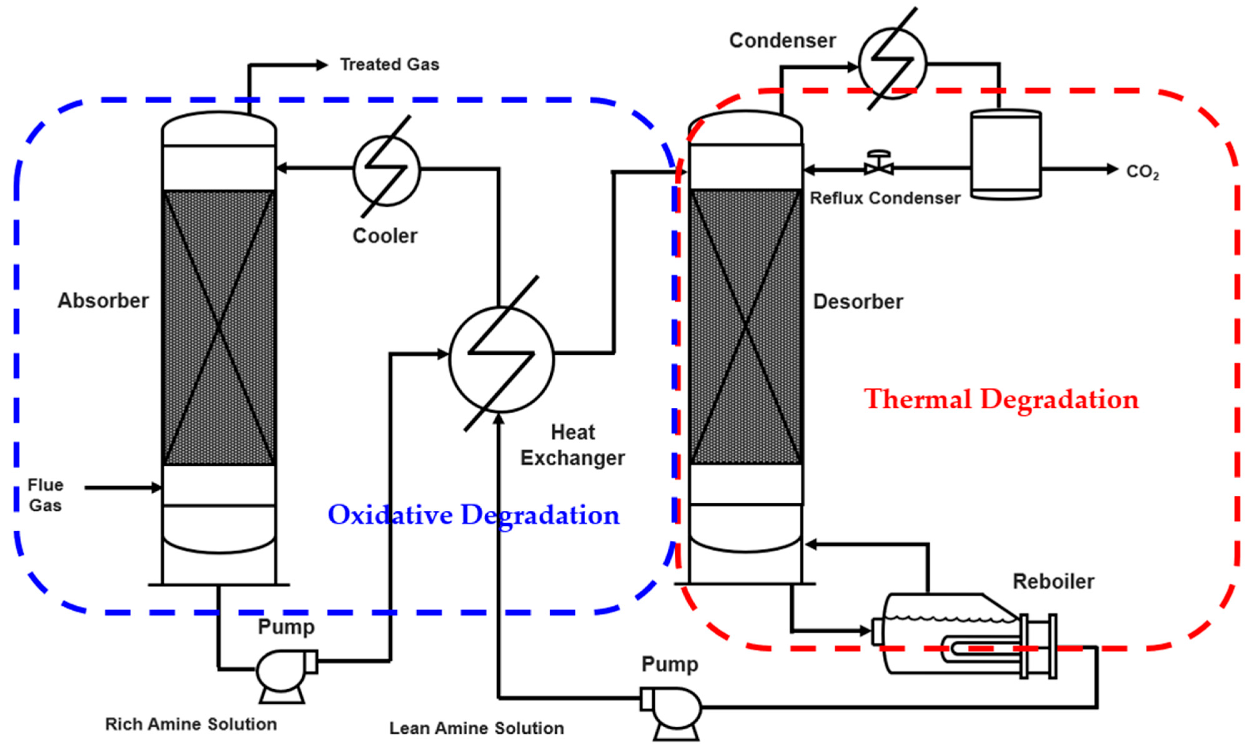
Figure 1. Typical CO2 absorption–desorption process using amine solution.
Sustainability 17 10311 g001
Figure 2. Architecture of ANN model used in current study.
Sustainability 17 10311 g002
Figure 3. Architecture of ANFIS model used in current study.
Sustainability 17 10311 g003
Figure 4. Architecture of RFR model used in current study.
Sustainability 17 10311 g004
Figure 5. Architecture of XGBoost model used in current study.
Sustainability 17 10311 g005
Figure 6. Performance of the ANN model for degradation of DMAE-PZ mixture. (a) train set for DMAE, (b) train set for PZ, (c) test set for DMAE, (d) test set for PZ.
Sustainability 17 10311 g006
Figure 7. Performance of the ANN model for degradation of MDEA-PZ mixture. (a) train set for MDEA, (b) train set for PZ, (c) test set for MDEA, (d) test set for PZ.
Sustainability 17 10311 g007
Figure 8. Performance of the ANN model for degradation of DEAE-PZ mixture. (a) train set for DEAE, (b) train set for PZ, (c) test set for DEAE, (d) test set for PZ.
Sustainability 17 10311 g008
Figure 9. Performance of the ANN model for degradation of TEA-PZ mixture. (a) train set for TEA, (b) train set for PZ, (c) test set for TEA, (d) test set for PZ.
Sustainability 17 10311 g009
Figure 10. Performance of the ANN model for degradation of DMAP-PZ mixture. (a) train set for DMAP, (b) train set for PZ, (c) test set for DMAP, (d) test set for PZ.
Sustainability 17 10311 g010
Figure 11. Performance of the ANFIS model for degradation of DMAE-PZ mixture. (a) train set for DMAE, (b) train set for PZ, (c) test set for DMAE, (d) test set for PZ.
Sustainability 17 10311 g011
Figure 12. Performance of the ANFIS model for degradation of MDEA-PZ mixture. (a) train set for MDEA, (b) train set for PZ, (c) test set for MDEA, (d) test set for PZ.
Sustainability 17 10311 g012
Figure 13. Performance of the ANFIS model for degradation of DEAE-PZ mixture. (a) train set for DEAE, (b) train set for PZ, (c) test set for DEAE, (d) test set for PZ.
Sustainability 17 10311 g013
Figure 14. Performance of the ANFIS model for degradation of TEA-PZ mixture. (a) train set for TEA, (b) train set for PZ, (c) test set for TEA, (d) test set for PZ.
Sustainability 17 10311 g014
Figure 15. Performance of the ANFIS model for degradation of DMAP-PZ mixture. (a) train set for DMAP, (b) train set for PZ, (c) test set for DMAP, (d) test set for PZ.
Sustainability 17 10311 g015
Figure 16. Performance of the RF model for oxidative degradation of PZ solution. (a) train set for PZ and (b) test set for PZ.
Sustainability 17 10311 g016
Figure 17. Feature importance test for input parameters to the RF model.
Sustainability 17 10311 g017
Figure 18. Cross-validation for RF model. (a) MAE per fold and (b) RMSE per fold.
Sustainability 17 10311 g018
Figure 19. Performance of the XGBoost model for oxidative degradation of PZ solution.
Sustainability 17 10311 g019
Figure 20. Feature importance test for input parameters to the XGBoost model.
Sustainability 17 10311 g020
Figure 21. Cross-validation for XGBoost model.
Sustainability 17 10311 g021
Table 1. Summary of the studies performed on amine degradation.
ModelSolventKey RemarksDescriptors/Inputs of the ModelReferences
QSPR model for degradation (not clear that it is oxidative or thermal) 22 different amine solutionsPLS model is used for this model
R2 value of 0.85
dipole moment,
calculated pKa value, and topological and Jurs descriptors
[11]
Machine learning model for thermal degradation135 data points for MEA solutionANN-PSO, Coupled simulated annealing-least squares support vector machine (CSA-LSSVAM), GEP and ANFIS used.
The most accurate model was ANFIS with R2, MSE, and AARE% of 0.992, 0.066, and 2.745.
CO2 loading, temperature, initial concentration of MEA, and duration[12]
Chemometric models for total inorganic carbon (TIC) and total alkalinity (TA) MEAPLS model is developed.
TIC-1 model was based on 1 latent variable (LV) with RMSE of 0.0415 mol/kg and R2 of 0.985. TA-1 model was based on 2 LV with RMSE of 0.0953 mol/kg and R2 of 0.882.
TIC-2 model was based on 3 LV with RMSE of 0.0206 mol/kg and R2 of 0.992. TA-2 model was based on 3 LV with RMSE of 0.0514 mol/kg and R2 of 0.920.
FTIR spectra data of the solvent samples[16]
Chemometric models to detect heat-stable salts (HSS) and amine degradation products (ADPs)MEAPLS model is developed.
HSS model was based on 1 LV with RMSE of 0.0144 mol/kg and R2 of 0.933. Another HSS model was based on 2 LVs with RMSE of 0.0117 mol/kg and R2 of 0.952.
ADO model was obtained with RMSE of 4621 mg/L and R2 of 0.916
FTIR spectra data of the solvent samples
Residual FTIR spectra
[17]
QSPR model for Oxidative degradation30 amines in 4 categories (cyclic and non-cyclic)Multiple Linear Regression (MLR) and CatBoost Regression (ML + MLR hybrid) used in the study. Based only on structural groups and substituents of amines with 22.2% average absolute deviations (AAD) for the training set and 7.0% AAD for validation set. Using CatBoost machine learning approach the degradation rate prediction accuracy improved to 0.3% AAD for the training set and 3.2% for validation.Structural descriptors (e.g., NH, CH, OH groups), electron-withdrawing groups (EWG), electron-donating groups (EDG), steric (S) variables, and interaction terms[20]
ANN modelCAER-solventANN for real-time estimation of alkalinity, carbon loading, and solvent degradation in amine-based CO2 capture. The key parameters used were pH, temperature, density, viscosity, and C/N ratio, all of which influence solvent performanceAmine concentration, temperature, CO2 exposure/flow, reaction time, measured alkalinity[21]
Table 3. Specifications of the XGBoost and RF Models.
XGBoostRF
ParameterDefinition/ValueParameterDefinition/Value
Number of inputs 14Number of inputs 14
Number of outputs 1Number of outputs 1
n_estimators1316n_estimators 444
Max depth10Max depth10
Learning Rate 0.0116Min samples split3
Subsample 0.6711Min samples leaf1
Colsample_bytree 0.9006Max_featuresLog2
gamma0.0013
Min_child_weight2
Reg_alpha 0.5034
Reg_lambda 0.5924
Table 2. Specifications of the ANFIS and ANN Models.
ANFISANN
ParameterDefinition/ValueParameterDefinition/Value
Number of inputs5Number of inputs5
Number of outputs2Number of outputs2
Fuzzy typeSugenoHidden layer size5
FIS generation GridPartitionTraining algorithmLevenberg–Marquardt
Optimisation methodHybridperformance functionMSE
Membership functionGaussianTransfer functionsTansig and purelin
Number of fuzzy rules9Max fail20
Maximum number of epochs300Number of epochs100
Initial step size0.01Initial Mu0.001
Increase rate of step size1.05Stopped Value Mu0.0001
Decrease rate of step size0.7
Table 4. Metrics for performance of ANN model for PZ-Tertiary Amines mixtures.
MetricsPZ-MDEAPZ-TEAPZ-DMAEPZ-DEAEPZ-DMAP
R2All-Output10.98030.97170.99390.98530.9969
R2All-Output20.97500.96260.98640.95930.9950
R2Train-Output10.98120.96880.99620.99380.9970
R2Train-Output20.98140.96900.97340.95580.9943
R2Validation-Output10.98090.98540.98780.99160.9977
R2Validation-Output20.92260.95700.99060.97340.9962
R2Test-Output10.97390.96950.99100.96240.9949
R2Test-Output20.92820.92720.99060.96580.9960
RMSEAll-Output10.09330.09670.06390.07890.0394
RMSEAll-Output20.09930.13490.08190.11480.0447
RMSETrain-Output10.09070.10690.04400.04580.0389
RMSETrain-Output20.09200.12790.06770.12610.0461
RMSEValidation-Output10.10260.05910.10640.06060.0368
RMSEValidation-Output20.08670.11430.13000.06930.0415
RMSETest-Output10.09500.07760.07950.16420.0438
RMSETest-Output20.13580.17740.07690.09770.0415
AARE%All-Output13.04%3.84%2.24%2.53%1.38%
AARE%All-Output29.82%11.06%10.17%7.26%2.42%
AARE%Train-Output12.90%4.48%1.23%1.39%1.38%
AARE%Train-Output29.24%11.98%10.02%7.95%2.32%
AARE%Validation-Output13.69%2.00%5.60%1.99%1.54%
AARE%Validation-Output211.64%9.92%11.63%5.07%2.71%
AARE%Test-Output13.00%2.88%3.34%8.09%1.21%
AARE%Test-Output210.57%8.15%9.37%6.38%2.58%
Table 5. Metrics for performance of ANFIS model for PZ-Tertiary Amines mixtures.
MetricsPZ-MDEAPZ-TEAPZ-DMAEPZ-DEAEPZ-DMAP
R2All-Output10.96790.98100.98930.99380.9975
R2All-Output20.95720.99360.99770.96040.9971
R2Train-Output10.99420.99870.99650.99800.9988
R2Train-Output20.99640.99710.99950.97280.9989
R2Validation-Output10.79190.94190.99150.99430.9936
R2Validation-Output20.79060.97340.99140.88200.9824
R2Test-Output10.97720.89130.72110.82560.9330
R2Test-Output20.99090.97550.97850.93100.9852
RMSEAll-Output10.11930.07920.08440.05130.0357
RMSEAll-Output20.13000.05570.03380.11320.0339
RMSETrain-Output10.05230.01950.04590.02820.0221
RMSETrain-Output20.03650.03860.01580.09320.0214
RMSEValidation-Output10.27780.18580.09310.06190.0739
RMSEValidation-Output20.31850.10960.06740.19350.0708
RMSETest-Output10.02080.08140.21450.12570.0273
RMSETest-Output20.01730.03480.05250.06880.0092
AARE%All-Output12.35%1.62%2.15%1.25%0.91%
AARE%All-Output23.26%3.92%2.98%4.93%1.27%
AARE%Train-Output11.35%0.65%1.37%0.85%0.52%
AARE%Train-Output22.09%2.38%1.02%2.71%0.79%
AARE%Validation-Output17.94%6.19%4.17%2.60%2.97%
AARE%Validation-Output29.39%10.90%2.90%8.12%3.82%
AARE%Test-Output10.66%1.84%5.20%2.26%0.68%
AARE%Test-Output22.88%4.69%19.34%17.90%1.03%
Table 6. Metrics for performance of RF and XGBoost model for oxidate degradation of PZ.
MetricsRFXGBoost
R2Train0.97220.9487
R2Test0.86550.8900
R2Validation0.88000.8890
RMSETrain0.09970.1354
RMSETest0.21770.2085
RMSEValidation0.24540.2230
AARE%Train1.65%2.61%
AARE%Test3.90%3.97%
AARE%Validation5.35%5.15%
5-fold cross validation (mean MAE)0.17350.1834
5-fold cross validation (std dev)0.02080.0132
Disclaimer/Publisher’s Note: The statements, opinions and data contained in all publications are solely those of the individual author(s) and contributor(s) and not of MDPI and/or the editor(s). MDPI and/or the editor(s) disclaim responsibility for any injury to people or property resulting from any ideas, methods, instructions or products referred to in the content.