Article

Nonlinear Relationships Between Urban Form and Street Vitality in Community-Oriented Metro Station Areas: A Machine Learning Approach Applied to Beijing

1
College of Architecture and Urban Planning, Beijing University of Technology, Beijing 100124, China
2
Jianguomen Sub-District Office of the People’s Government of Dongcheng District, Beijing 100005, China
*
Author to whom correspondence should be addressed.
Sustainability 2025, 17(22), 10278; https://doi.org/10.3390/su172210278
Submission received: 9 October 2025 / Revised: 5 November 2025 / Accepted: 12 November 2025 / Published: 17 November 2025
(This article belongs to the Section Sustainable Urban and Rural Development)

Abstract

This study investigates the nonlinear, interactive, and temporally dynamic effects of urban form on street vitality within community-oriented metro station areas (MSAs) in Beijing. It offers potential reference value for other cities facing comparable challenges in MSA implementation and increasing motorization. This research addresses gaps in prior studies concerning the integration of multi-source data, nonlinearity, and diurnal variation. Utilizing an extended node-place-design framework, urban form is conceptualized through network, interface, and functional dimensions. The empirical analysis employs multi-source datasets, including 128,199 mobile device trips recorded in April 2024, OpenStreetMap for network data, Baidu points of interest for functional data, and Grasshopper for interface metrics, covering 183 street samples within a 1000 m radius of metro stations. Traditional regression models—such as ordinary least squares and spatial autocorrelation and cross-correlation—are used as baselines, while a novel gradient-boosting decision tree with latitude and longitude features is applied to enhance predictive performance. The results indicate that key contributors include road network density (16.89%), road intersections (10.56%), and point-of-interest density (9.74%), with Shapley Additive Explanations dependence plots demonstrating nonlinear thresholds. The analyses reveal synergistic or antagonistic interactions among features. Temporal fluctuations in feature importance further support the presence of diurnal dynamics. The study provides insights for time-sensitive urban planning aimed at enhancing MSA vitality, sustainability, and resident quality of life, while acknowledging that the conclusions are context-specific to Beijing and require additional validation in other urban environments.

1. Introduction

1.1. Background and Significance

Urban vitality is a cornerstone concept in urban studies, widely recognized as a key indicator of high-quality urban space and a primary goal of urban design [1]. This concept refers to the capacity of urban spaces to attract diverse groups of people to participate in a variety of activities throughout the day, which fosters abundant human interactions and a vibrant public environment. As it is closely linked to urban design and urban sustainability, urban vitality has been increasingly regarded as a measure of urban prosperity and quality of life. Moreover, increased vitality is one of the most desirable outcomes of transit-oriented development (TOD). In cities, metro station areas (MSAs) are among the densest and most populated locales [2,3]. In contrast to conventional TOD contexts, research on vitality has paid little attention to MSAs, which are often characterized by a high density of business, social, and community facilities, as well as various daily activities [4,5]. The vitality of an MSA depends partially on the features of its built environment [6]. With accelerating urbanization, MSAs have gradually become critical nodes in urban development. Optimizing urban spatial forms, rationally planning urban functions, and enhancing the design of street spatial forms are essential for the development of MSAs.
Community-oriented MSAs are a type of TOD centered around rail stations, and they are primarily designed to serve the daily needs of the surrounding residential community [7,8]. However, the forms of these MSAs are especially susceptible to severe environmental decay, social disorder, and pronounced declines in vitality. Therefore, a comprehensive understanding of these variations is crucial for capturing the long-term influence of urban spatial form features on residents’ daily lives.

1.2. Literature Review

1.2.1. Vitality and Its Measurements

Scholars have defined vitality from diverse perspectives. Vitality is generally considered to refer to the quality of a space in a city that attracts diverse groups of people to participate in a wide range of activities at different times of the day [9,10]. The concept of vitality is primarily based on the work of Jane Jacobs [1], and contemporary research has extended this concept to incorporate dimensions of temporal rhythm. Other scholars consider vitality to be a socio-spatial construct that can be understood as a set of immaterial activities [11,12] that can be measured from its social aspect through “recreational and social activities” [13].
With the recent emergence of travel-related big data, many researchers have also begun to employ indicators representing the intensity of socio-spatial activity to measure vitality [14]. Various types of location-based service positioning data have been used to derive indicators of urban street vitality based on crowd activity intensity. These new approaches utilize advanced data sources, including metro rail ridership, social media check-ins, mobile phone signaling, street-view imagery, and positioning records, to enable multidimensional and real-time assessments of vitality across spatial and temporal scales.

1.2.2. Urban Form Features Influencing Vitality

Urban form refers to the physical and spatial configuration of human settlements, encompassing a multidimensional set of characteristics that define the structure, layout, and pattern of urban areas [15]. This concept encompasses morphological attributes such as density, mixed land use, street connectivity, accessibility, block size, and the distribution of green spaces, as well as three-dimensional building arrangements and architectural features [16,17]. In contemporary urban studies, its definition has expanded to incorporate configurational and perceptual qualities—such as walkability, scale, enclosure, and visual coherence—all of which together influence human behavior, environmental performance, and socioeconomic functionality [18,19,20]. This study conceptualizes urban form as a multidimensional construct quantified through key metrics across three domains.
Research on urban forms has shifted from a focus on only physical space to the interactions between people and their environment [21,22]. Emphasis now lies on how individuals perceive, comprehend, and utilize urban spaces. Existing studies have explored how favorable urban forms stimulate and sustain human vitality within cities from multiple dimensions and perspectives. Qualitative principles such as coherence, imaginability, and transparency, which have been established as measures of good urban form, have also been linked to human vitality [23,24].
However, although these qualitative principles offer a critical theoretical foundation, their practical application often encounters challenges related to subjectivity and difficulties in quantification. To bridge the gap between theoretical concepts and design practice, recent studies have increasingly aimed to translate descriptive urban form principles into quantifiable morphological indicators and to empirically examine their statistical relationships with human vitality [25,26,27,28]. Parametric design platforms such as Grasshopper, Dynamo, and Blender have also been employed to analyze human–environment interactions, revealing that metrics like interface density and alignment ratio are context-dependent.
A substantial body of research has explored the relationship between urban form and vitality; however, the methodological approaches of this research often rely on a single data source [29,30]. Studies utilizing points of interest (POI) or land use data in geographic information systems (GIS), for example, commonly use functional density and diversity as proxies for vitality. While these static datasets effectively capture the spatial potential for activity, they do not reflect the actual, dynamic presence of people. Conversely, studies employing GPS trajectories or mobile phone signaling data are effective in mapping the real-time distribution and flow of populations across urban space [31]. Nonetheless, these mobility-centric approaches frequently lack semantic richness, offering limited insight into the purposes or qualitative aspects of the observed activities. This may result in superficial interpretations and an inability to account for contextual factors such as user intent or environmental interactions. Complementary methods, such as field observations and questionnaire surveys of street interfaces, provide rich behavioral and perceptual insights but are inherently limited in terms of scalability and temporal resolution. This underscores the necessity for integrative, multi-source analytical frameworks.
The integration of these diverse analytical methods has enabled increasingly precise investigations into the complex relationship between street spatial design and urban vitality.

1.2.3. Nonlinear Relationship Between Urban Form and Vitality

Building on the development of multidimensional measurement methods for street vitality and built environment characteristics since the 1990s, the theoretical literature on urban vitality generally supports the view that urban spatial form and vitality are correlated [32,33].
Research exploring the relationship between urban vitality and the built environment has primarily employed linear modeling approaches, utilizing both statistical and GIS-based techniques. A substantial body of literature has applied regression methods to identify key environmental determinants. For instance, ordinary least squares (OLS) regression has been widely used to demonstrate that urban vitality may be enhanced through targeted environmental design strategies [34,35,36]. While OLS offers advantages in simplicity, interpretability, and computational efficiency, it is constrained by assumptions of linearity and independence and, as a result, often fails to account for spatial autocorrelation or heterogeneous effects across urban areas. To address these limitations, spatial econometric models such as the spatial autocorrelation (SAC) model have been developed. Additionally, to address the issue of spatial non-stationarity inherent in global models, geographically weighted regression (GWR) has been employed to capture localized effects of built environment variables [37,38]. These regression models are valued for their interpretability but are limited in their capacity to quantify complex synergies or nonlinear thresholds.
Recent studies suggest that landscape characteristics and features of urban form exhibit nonlinear relationships with vitality [39,40]. Scholars have increasingly turned to machine learning-based methods to investigate such nonlinearities [41,42]. Models such as random forest (RF) and extreme gradient boosting (XGBoost) have been used to assess the relative importance of various factors influencing spatial vitality [43,44,45]. Despite their strong predictive capabilities, these machine learning approaches often suffer from limited interpretability and theoretical transparency. Furthermore, their outputs are highly sensitive to parameter tuning and the representativeness of input data, which may hinder the generalizability of findings across diverse urban contexts.
Although rarely emphasized, a number of studies have also suggested synergistic effects among urban form variables. For example, a study in Yantai identified a multiplier effect in activity generation across functionality, building form, accessibility, and human perception [46]. Other research has shown that merely increasing road network density in TOD areas does not necessarily enhance vitality; rather, optimizing land use allocation and applying moderately differentiated functional distributions with high accessibility are more effective strategies [47]. Additional findings suggest that high-quality transit combined with supportive land development produces synergistic effects in promoting urban vitality [48]. These studies offer preliminary evidence for potential interactions among spatial accessibility, land use type, and functional richness in shaping street vitality. However, such interaction effects have been largely overlooked, primarily due to difficulties in measuring interaction intensity within generalized linear or hybrid models.
In summary, empirical investigations into the nonlinear and interactive relationships between urban form and vitality remain nascent and lack comprehensive validation. Moreover, limited attention has been paid to explaining the underlying mechanisms that drive these nonlinear dynamics.

1.2.4. Research Gaps

To optimize metropolitan development and spatial performance, it is imperative to investigate how the evolving urban forms of MSAs nonlinearly and synergistically influence street vitality. There is limited available research regarding the characteristics of the layout of MSAs. There are three primary gaps in related research:
Gap 1: The prevailing research paradigm, characterized by fragmented data sources and linear modeling approaches, has substantially constrained the investigation of the complex, nonlinear relationships essential to a deeper understanding of urban vitality.
Gap 2: There is insufficient attention to the temporal dynamics in the relationship between street vitality and urban form. Beyond seasonal or periodic variations, significant diurnal patterns can also be observed and merit further exploration.
Gap 3: Existing studies have rarely disentangled definitive interactive effects among built environment variables from their individual effects.

1.3. Theoretical Hypothesis

Across different perspectives, sustaining street vitality requires a dense and diverse population that is continuously engaged in a broad spectrum of activities. As a planning framework for the desired development of land use and transport, TOD often emphasizes multiple physical characteristics, including high density, mixed land use, amenity richness, a pedestrian- and cyclist-friendly environment, and accessible transit. These characteristics have been theoretically linked to street vitality [49].
This study builds upon the conventional node–place model by incorporating an additional interface dimension and employs this extended model to conduct a detailed evaluation of walking environments within MSAs. The node–place model serves as a foundational conceptual framework in urban planning and transportation research, particularly within the context of TOD studies [50]. The “node” dimension emphasizes transport connectivity, network centrality, and accessibility within the metro system. Conversely, the “place” dimension focuses on the livability and functionality of the station area, typically assessed using indicators such as land use intensity, functional diversity, and the availability and variety of public service facilities. Multivariate indicator systems are often used to quantify node and place performance in station areas, with bivariate scatter plots commonly employed to illustrate competitive or synergistic relationships between these dimensions.
However, conventional applications of the node–place model have often failed to account for the role of urban design in mediating transportation and land use interactions [51,52,53]. In response, recent research has increasingly emphasized the importance of incorporating micro-scale environmental factors—such as walkability [54,55], street design attributes [56], and urban morphology [57]—thereby revealing a significant limitation in the traditional framework.
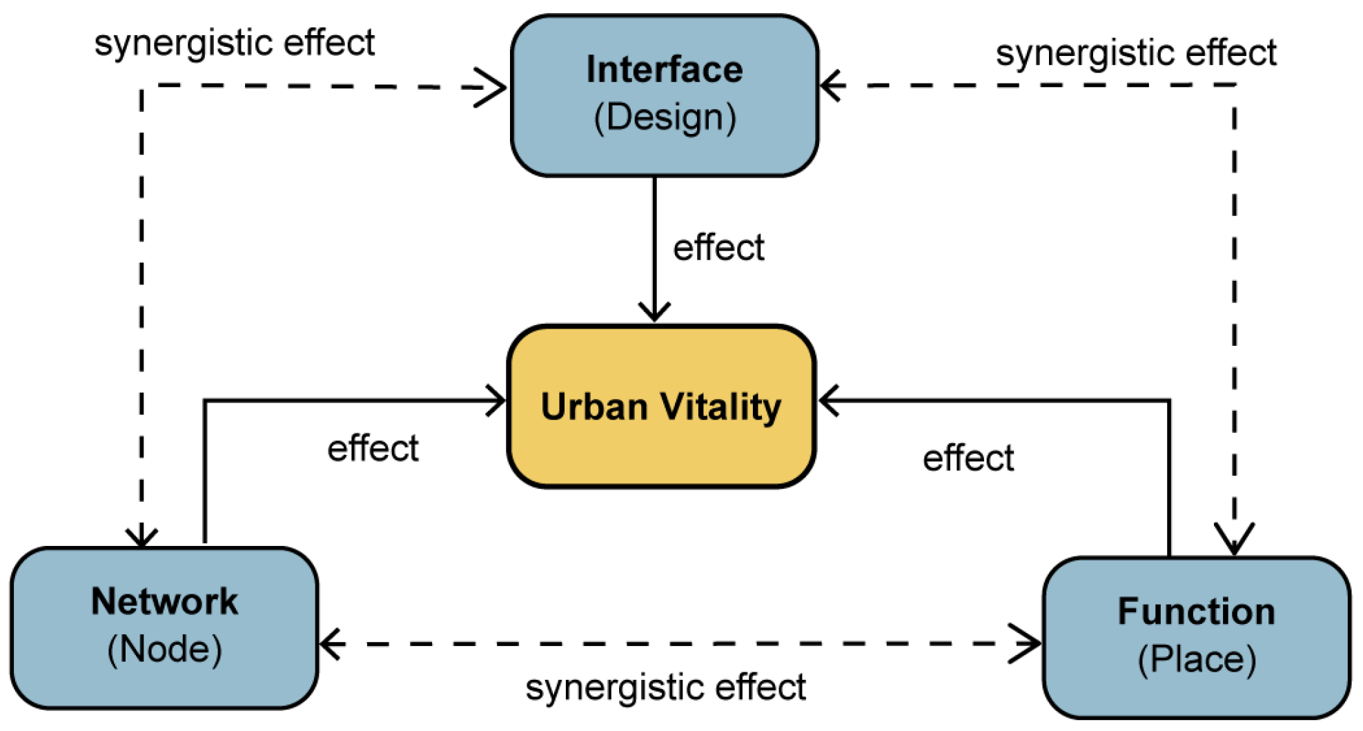
In light of the above, this study extends the classical node–place framework through the integration of a design dimension, transforming the original two-dimensional structure into a three-dimensional evaluative space (Figure 1). This enhanced model is then applied to conduct a detailed assessment of urban form characteristics in MSAs. The model is applied as an analytical approach for investigating the interaction between transportation, walking friendliness, and land use around station areas. It provides a rational framework for better understanding the relationships between MSA’s urban form and street vitality, based on three key dimensions: network (node), interface (design), and function (place).
Within this framework, the present study investigates MSAs in Beijing, China, across different time intervals throughout the diurnal cycle. The following hypotheses are proposed concerning the relationship between urban form and street vitality:
Hypothesis 1: 
The relationship between key urban form characteristics—such as road network density, road intersections, and aspect ratio—and street vitality is nonlinear, exhibiting identifiable activation and threshold effects beyond which their influence diminishes, stabilizes, or reverses.
Hypothesis 2: 
Urban form features do not function independently but interact with one another, producing either synergistic effects (between functional and network dimensions such as POI and transit density) or antagonistic effects on vitality.
Hypothesis 3: 
The magnitude and nature of urban form’s influence on vitality are temporally dynamic, varying across different times of day. Network features may exert greater influence during commuting periods, while functional indicators may predominate during non-peak leisure periods.

2. Materials and Methods

2.1. Materials

2.1.1. Study Area

This study defines MSAs using a 1000 m radius, which is sufficiently large to include the primary mode of access and the spatial influence zone of each station. This definition is characterized by the MSA outlined in the Opinions on Further Improving the Compilation and Management of Integrated Planning Schemes for Rail Transit Lines in Beijing [58]. This officially recognized standard also aligns with the behavioral concept of a 15 min walking catchment, ensuring methodological consistency with both regulatory frameworks and urban mobility research. This resulted in a final dataset comprising 183 street samples (Figure 2).

2.1.2. Street Vitality

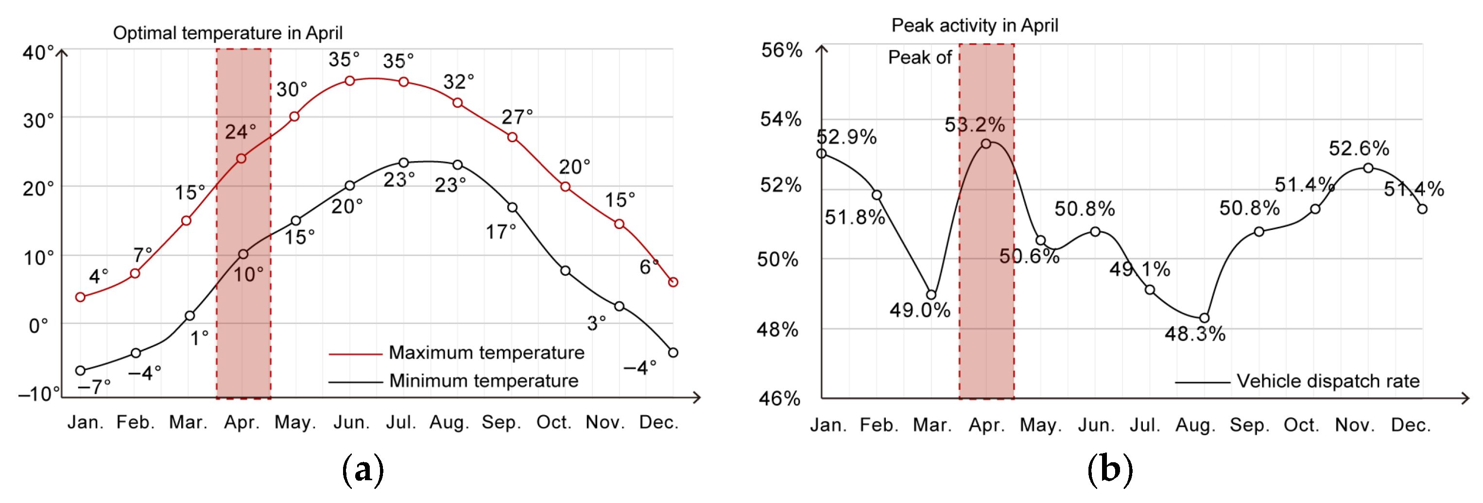
As indicated by the red squares in Figure 3a, real-time monitoring data from the Beijing Meteorological Observatory indicate that April offers the most favorable climate conditions for outdoor activity, with an average daily temperature of 16.3 °C, aligning with the Universal Thermal Climate Index for human comfort. Furthermore, statistics from the Beijing Transport Institute (2024) [59] confirm that April experiences the highest level of outdoor transportation activity in the city (Figure 3b). To ensure the reliability of behavioral observations, this study selected 18, 19, and 20 April 2024, as data collection dates. These dates were chosen to avoid the influence of irregular events (such as holidays) and include both weekdays and weekends. To minimize temporal noise, this survey was confined to a short, contiguous period. This strategy controlled for confounding temporal variables, including transient weather conditions, long-term seasonal trends, and special events, thereby strengthening the study’s ability to attribute observed vitality variations to spatial design features instead of temporal fluctuations. The dataset was composed of geographical location data from personal mobile devices. Data were collected continuously from 00:00 to 24:00, with approximately one data point recorded each hour. The final dataset contained 128,199 trips.
The spatial vitality assessment involved five methodological steps [60].
First, Python 3.12.5 was used to extract vector heat map data (Figure 4) representing hourly crowd activity ( P v ), based on point samples within a 4-hectare square area ( S o ). Second, the raw data were cropped, georeferenced, and projected. Using QGIS, a ‘Fishing Net’ grid was applied to generate buffer zones and convert point data into surface data.
P o = P v / S o / N
Third, road network data were imported, and corresponding road centerlines were identified by street name. Buffer zones were then established based on road classification criteria. Fourth, the intersecting vector tool was used to overlay road samples with heatmap buffer zones. The heat data were normalized and spatially assigned to the corresponding road segments. Finally, the Interquartile Range method in Python was applied to filter and integrate the data.
As illustrated in Figure 4, both the mean and total heat values demonstrate a consistent pattern in which weekdays (Figure 4a) exhibit higher levels than weekends (Figure 4b). However, the standard deviation of weekend heat value is 52.12, which is higher than that of weekdays (46.42), indicating a greater variability in population activity during weekends. Such fluctuations may result from reduced commuting effects during weekends, leading to altered spatial aggregation patterns and, consequently, a decrease in weekday population activity intensity.
Three factors were comprehensively considered in selecting representative time points within the day–night cycle for analysis. These include:
  • The temporal representativeness of the selected periods, according to the daily mean value, ensures coverage of both morning and evening peak hours as well as midday off-peak hours;
  • The relative peak values in crowd activity density across time intervals;
  • The general distribution of outdoor population presence throughout the day.
Accordingly, this study selected 9:00, 15:00, and 21:00 as the observation points for analyzing spatial vitality. These time slots exhibit relatively stable values and heightened neighborhood vitality, facilitating clearer insights into variations in crowd activity patterns during morning, afternoon, and evening periods.

2.1.3. Urban Form Characteristics

Network and Functional Data
Urban street network data were primarily extracted from OpenStreetMap, encompassing road classifications, building footprints, and land use types. Roads were categorized into four classes: expressways, arterial roads, collector roads, and local streets. Theoretical road spacing standards, as outlined in the Standard for Urban Comprehensive Transport System Planning, served as the foundational reference [61]. Field surveys were conducted to verify the consistent implementation of these spacing standards within the built environment. Corresponding buffer zones were delineated from the street centerlines, with widths of 80 m, 60 m, 40 m, and 20 m, respectively, to comprehensively capture the spatial influence on both sides of each road category (Figure 5). The analysis of functional data was based on Baidu POI data, with functional mixedness calculated using an information entropy model. Spatial analyses were performed using the QGIS platform, and the acquired vector data were stored in a spatial database to establish an integrated spatial data management system. Spatial statistical techniques were subsequently applied to quantify a series of network indicators. Data processing and indicator standardization were conducted using the Pandas library in Python.
Interface Data
Regarding façade morphology, which entails complex three-dimensional spatial operations, this study employed Baidu building data in conjunction with the Grasshopper parametric platform to perform three-dimensional projection and spatial topological analysis. This approach enabled the precise extraction of architectural façade morphological characteristics, which were subsequently used to assess the regularity of street interfaces. Due to the computational complexity of morphological analysis, all quantitative evaluations were conducted using a parametric cluster macro calculator developed by the authors within Grasshopper (Figure 6).
Following a systematic description of the data sources and processing methods related to street networks, interface morphology, and functional composition, this study integrates these elements to construct a comprehensive quantitative indicator system for street morphology (Table 1). A summary of the analyzed sample data is presented in Appendix A, Table A1.

2.2. Methods

2.2.1. Correlation Between Variables

Pearson correlation analysis was employed to examine the relationship between the intensity of human spatiotemporal activity and spatial morphological variables. The Pearson correlation coefficient (PCC) ranges from −1 to 1. A value approaching 0 indicates that there is no linear correlation between variables, while a value approaching −1 indicates a strong negative correlation, and vice versa [66].
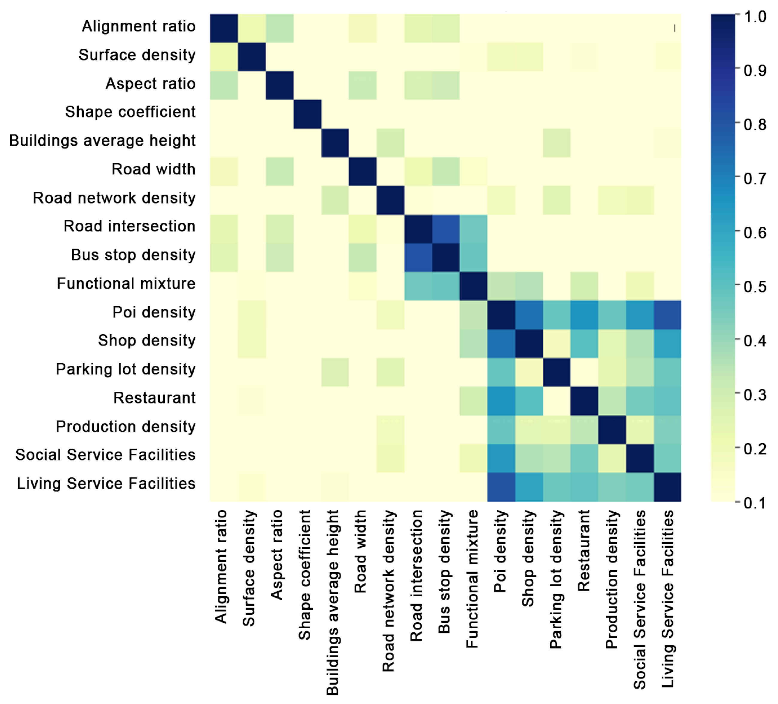
Correlation analysis was conducted on the 17 urban form indicators to identify the relationships between features and eliminate highly correlated ones. This mitigated potential multicollinearity issues and improved the stability and interpretability of subsequent models. Based on the results (Figure 7), this study establishes a street spatial form evaluation index system tailored to community-oriented MSAs, consisting of 3 first-level indicators and 17 s-level indicators. The subsequent analysis employs 17 urban form indicators as independent variables and street vitality as a dependent variable to compare the performance of traditional linear regression and machine learning models in predicting urban vitality.

2.2.2. Traditional Regression Models

Despite its lower predictive accuracy compared to machine learning models, traditional linear regression remains valuable for exploring the relationship between urban form and vitality due to its interpretability and parsimony. This study thus employs linear models as a baseline for a comparative analysis with more complex, nonlinear alternatives. To investigate the relationship between urban spatial form and spatiotemporal behavior, the study initially applies traditional OLS models as a baseline analytical approach [67]. However, its applicability is limited in spatial analyses, as it assumes that error terms are independently and identically distributed. This assumption often fails in spatial contexts, resulting in biased estimates.
Given that urban spatial form and vitality exhibit spatial dependence and are influenced by geographic proximity, the study further introduces the spatial autocorrelation and cross-correlation (SAC) model. This model addresses spatial dependence by incorporating spatial lag effects and spatial error terms. The Lagrange multiplier (LM) test can detect significant spatial autocorrelation. Therefore, the SAC model is more appropriate for spatial data analysis.
Table 2 summarizes the results of the OLS and SAC models at different time points. At all three time points, the LM tests for both spatial lag and spatial error in the OLS model yielded significance levels below 5%, indicating strong spatial dependence. Additionally, the Akaike Information Criterion (AIC) values for the SAC model are consistently lower than those for the OLS model across all time periods. The SAC model also demonstrates reduced prediction error and substantially higher explanatory power. Due to these observed differences in coefficient magnitude and statistical significance between the OLS and SAC models, subsequent analysis and discussion will focus exclusively on the SAC model results.

2.2.3. Machine Learning Models

This study applies four widely used machine learning algorithms in urban form correlation analysis: RF, gradient boosting decision tree (GBDT), extreme gradient boosting (XGBoost), and light gradient boosting machine (LightGBM) [68,69,70]. To evaluate model performance, four standard regression metrics are used: mean squared error (MSE), root mean squared error (RMSE), mean absolute error (MAE), and the coefficient of determination (R2).
The scikit-learn Python library was used to implement the models with default parameters [71,72]. Grid search is employed to address the potential randomness associated with hyperparameter tuning and model training (Table A2). The training process consists of the following steps: (1) Defining Hyperparameters; (2) Generating Parameter Grid; (3) Cross-Validation; (4) Score Comparison; (5) Final Training, retraining the model using the entire training dataset under the optimal hyperparameter configuration; (6) Independent Testing; and (7) Model Selection and Visualization. This representative model is then analyzed further (Figure 8). Through testing, we found that setting n_estimators = 100, learning_rate = 0.1, max_depth = 3, and random_state = 42 yielded the highest R2 value of 0.745 for GBDT, indicating superior model performance (Table 3). These parameters were selected based on their ability to balance model complexity and generalization.
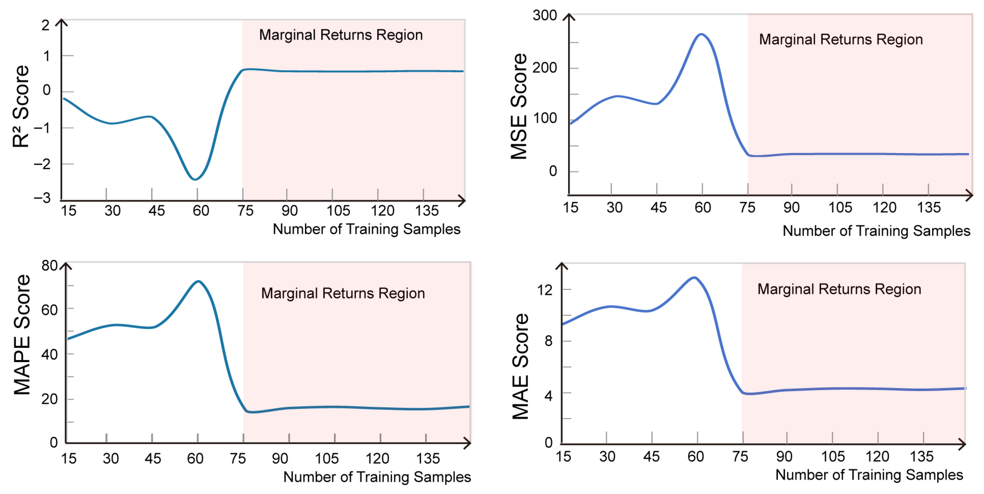
To validate the sufficiency of our dataset, we plotted the learning curves for the GBDT model, as shown in Figure 9. The curves demonstrate that both the training and validation performance converge as the sample size approaches the full dataset.

2.3. Technical Workflow

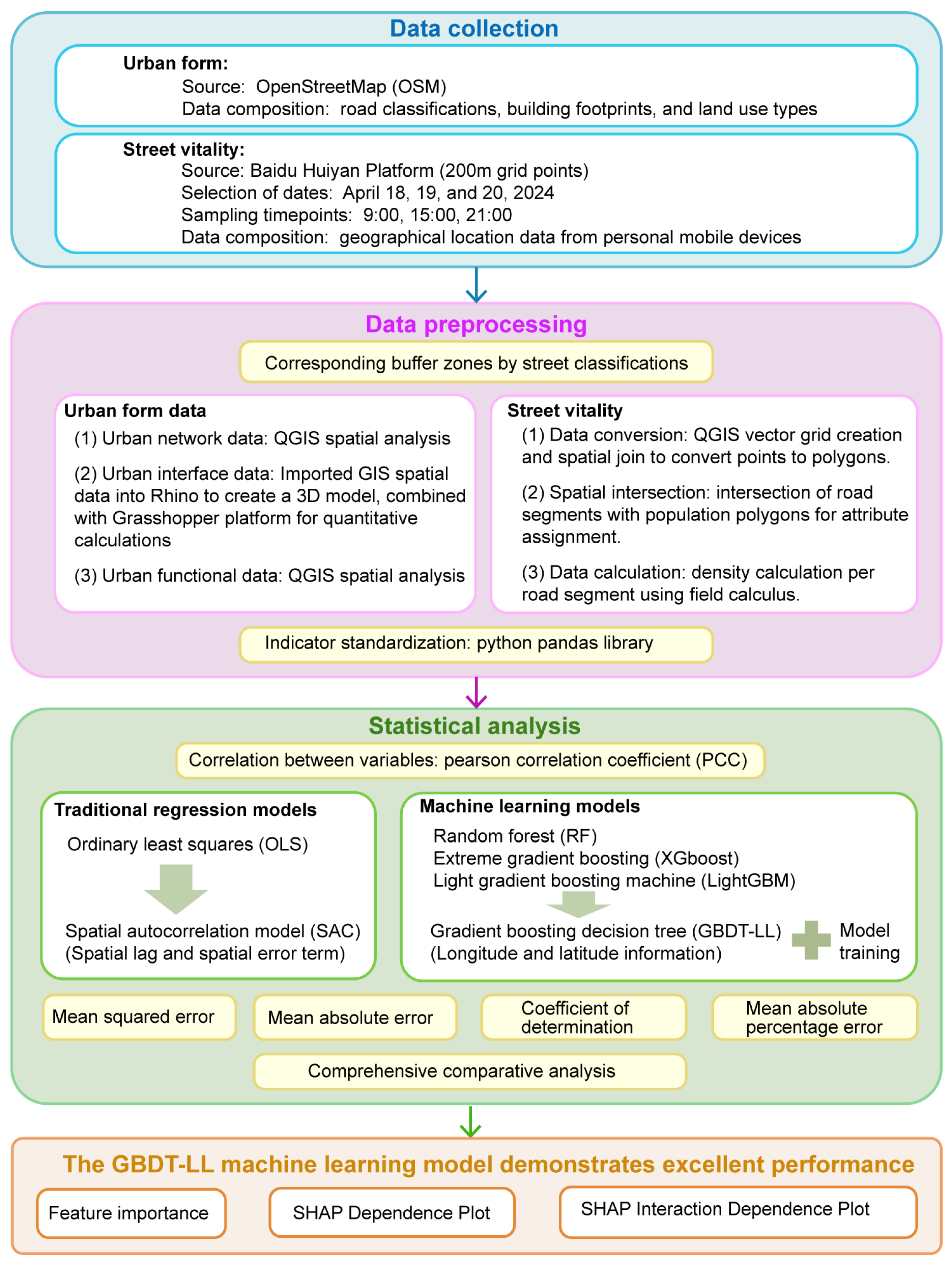
The research methodology was structured into four sequential phases to systematically investigate the nonlinear relationships between urban form and street vitality, as follows:
  • Multi-source data collection;
  • Data preprocessing, urban form, and street vitality calculation;
  • The application of two analytical techniques to analyze these relationships and interpret them;
  • The leveraging of feature importance, SHapley Additive eXplanations (SHAP) dependence plots, and SHAP interaction dependence plots for comparative analysis, synthesis, and hypothesis validation.
The integrated technical workflow is detailed in Figure 10.

3. Results

3.1. Performance of Machine Learning and Traditional Regression Models

To enable comparisons with the SAC model and control for the spatial factor variable, the study introduced coordinate information (latitude and longitude) as a general variable into the GBDT model, constructing the GBDT-LL model. Specifically, the spatial context of the observations was encapsulated by incorporating the geographic coordinates of the street segment centroids. These centroid locations were algorithmically determined from the street geometry within a GIS environment by utilizing the WGS 84/Pseudo-Mercator (EPSG:3857) coordinate reference system. Latitude and longitude were included as independent variables in the analysis. This setup allows the SAC and GBDT-LL models to be contrasted in terms of their treatment of spatial factors. The introduction of geographic information also improves model accuracy.
Table 4 presents the predictive performance of six models—OLS, SAC, RF, XGBoost, LightGBM, and GBDT-LL—across different time points. Compared with the OLS baseline, the machine learning models demonstrated an advantage. Although the observed improvements may not meet conventional thresholds for statistical significance, they indicate practical relevance, particularly in the context of urban vitality forecasting, where data volatility is high. These findings suggest that machine learning approaches are better suited to capturing complex, nonlinear relationships in this domain.

3.2. Feature Importance in Machine Learning Models

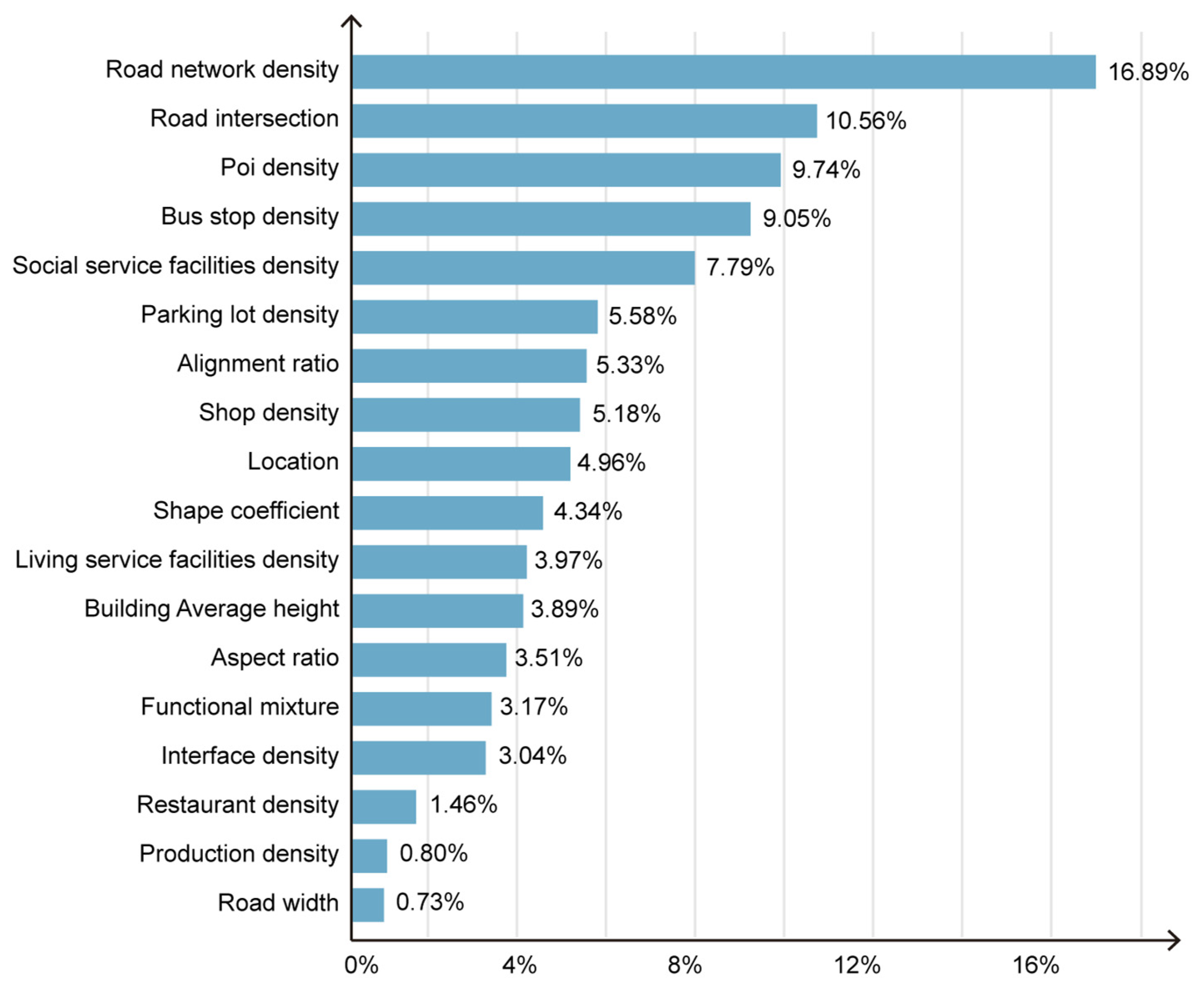
Feature importance quantifies the contribution of each independent variable to the prediction of the dependent variable within a machine learning model. It highlights the most influential variables in determining model outcomes [73]. This study assesses the relative importance of 17 street spatial element variables in terms of their contribution to the model’s predictive accuracy (Figure 11).
Road network density (16.89%), road intersections (10.56%), POI density (9.74%), bus stop density (9.05%), and social service facilities (7.79%) are the dominant contributors to vitality around MSAs.
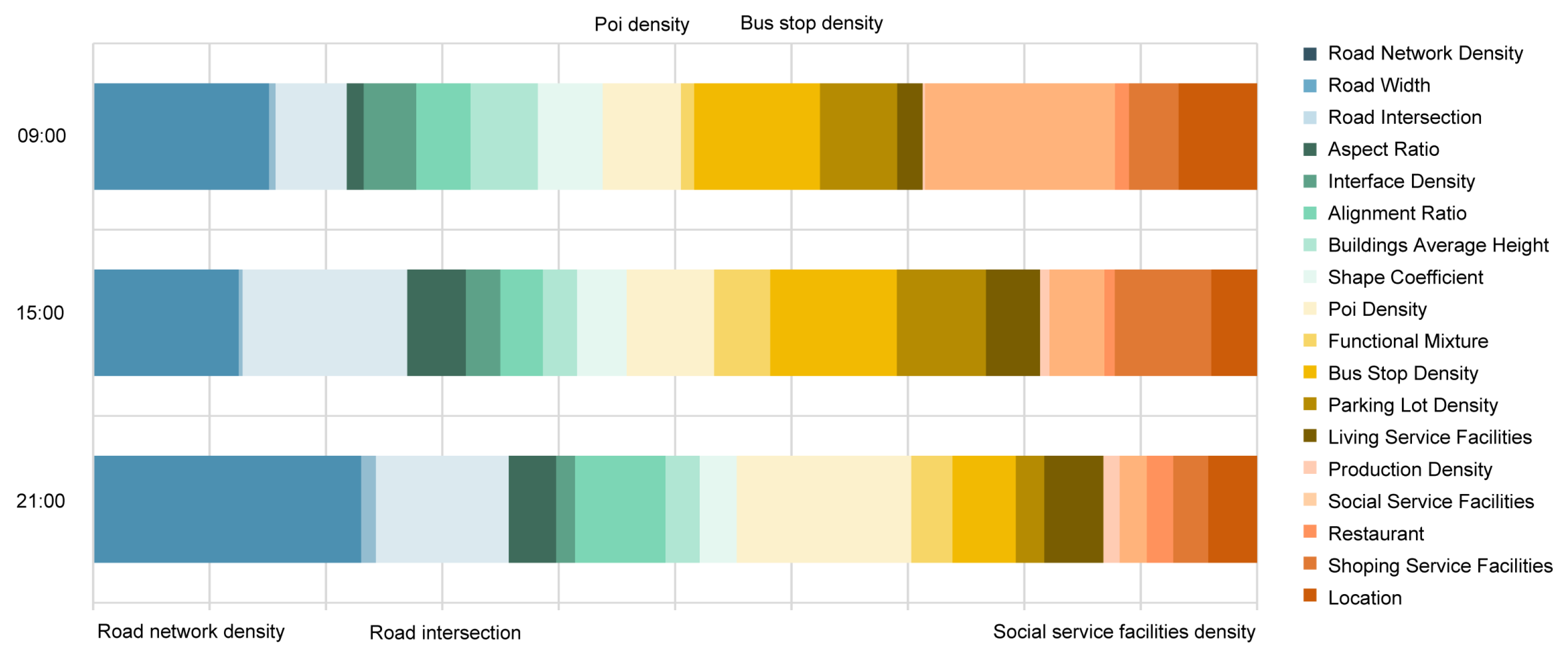
To compare the relative contribution of features across different times of day, we converted the SHAP feature importance values into percentage contributions and visualized them using a stacked bar chart (Figure 12). This visualization highlights how the influence of each feature shifts in proportion to the total throughout the diurnal cycle.
These urban form features serve as the key mediators and essential prerequisites for the generation of high-activity MSAs. The model developed in this study quantifies this synergistic relationship. According to the feature importance analysis derived from the GBDT-LL model, the street spatial form dimensions exert varying levels of influence on vitality depending on different times of the day. In the network form, road density and intersection frequency are critical during peak commuting hours. In the interface form, aspect ratio and building height significantly impact pedestrian comfort and safety during evening hours. In the functional form, functional and service facility density are especially influential during the period between 15:00 and 21:00. These variations in feature importance reflect the dynamic temporal nature of urban spatial configurations, providing empirical support for enhancing urban planning and design.
The subsequent section discusses the top five urban form features with the most significant magnitude of fluctuation. Findings suggest that the influence of network structure indicators on vitality dependency values is strongly demand-driven. At 9:00 and 21:00, the feature importance of network-related variables, such as road network density and the number of intersections, is substantially higher than that of other spatial dimensions. This reflects the heightened demand for transportation accessibility during commuting hours, where dense, well-connected road networks effectively accommodate both pedestrian and vehicular flow, thereby reducing transit times. By 15:00, traffic volume decreases, and the significance of network density diminishes accordingly. However, by 21:00, the importance of density increases once again, likely due to the rise in evening activities in high-density neighborhoods. Bus stop density exhibits peak influence at 9:00, underscoring commuter preference for public transit systems. Its importance diminishes in the afternoon and evening, though it retains moderate influence during nighttime travel.
Functional indicators exhibit temporal variation consistent with an activity gradient, shifting from a focus on accessibility in the morning to an emphasis on functional diversity and spatial concentration in the afternoon and evening. At 9:00, the influence of functional density on behavioral vitality is limited, as the transportation network primarily drives commuting behaviors. However, by 15:00, the role of functional density increases considerably, especially in areas with commercial and recreational facilities, which become more attractive. At 21:00, the influence of functional density reaches its peak, as nighttime activities concentrate in areas with dense functional offerings.
At 9:00, urban vitality is primarily necessity-driven, with social service facilities acting as rigid destinations and thus exhibiting peak feature importance. In contrast, at 15:00 and 21:00, vitality is shaped by discretionary, leisure-oriented activities, which diminish the influence of social services. Conversely, the density of dining and entertainment facilities peaks at night, becoming the dominant factor enhancing neighborhood attractiveness and drawing substantial amounts of activity.

3.3. SHAP Dependence Plots

SHAP dependence plots visualize the influence of urban form factors on street vitality by illustrating the relationship between feature values and their corresponding SHAP values (Figure 13). The locally weighted scatterplot smoothing (LOWESS) algorithm was employed to elucidate potential threshold effects [74].
Figure 13a–d provide strong evidence of threshold effects in the relationship between urban form and street vitality within community-oriented MSAs. Due to the large number of urban form features, only variables with significant feature importance are presented. Within their respective effective ranges, the number of road intersections (22–28 per km2) and road network density (14–16 km per km2) positively influence crowd activity during peak periods. Beyond these thresholds, the positive impact plateaus. A similar trend is observed for bus stop density (1–7 units per km2) and POI density (14–100 units per km2), which maintain a positive correlation before stabilizing.
Figure 13e,f show that variables such as aspect ratio and average building height display different behavior. These features exhibit a noticeable negative correlation beyond certain thresholds. Specifically, the positive impact of aspect ratio stabilizes around 0.5, after which it begins to decline. When the aspect ratio exceeds 2, it has a negative impact on street vitality. A comparable pattern is observed for the average building height, with positive effects increasing beyond 20 m and peaking at approximately 42, followed by a decrease.
In contrast, as for Figure 13g,h, for street width, vitality increases between 10 m and 15 m, plateaus and turns negative between 15 m and 40 m, and shows a tentative rebound beyond 40 m. When parking density is below 1 unit per km2, it promotes street vitality but declines steadily. The effect diminishes with increasing density and reverts to negative beyond it, with only a marginal recovery observed after 4.5 units per km2.

3.4. The Interaction Effects Between Key Urban Form Variables

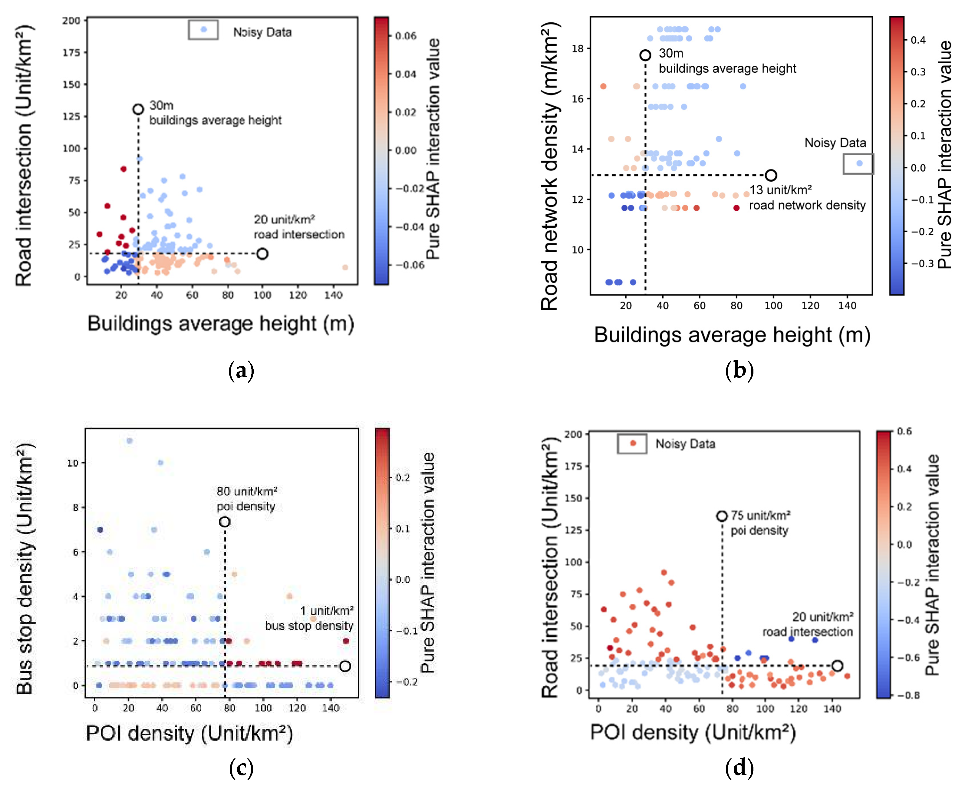
SHAP is used to visualize how the contribution of one feature depends on the value of another [75]. Each sample is represented as a point, with one feature’s value plotted on the x-axis and another feature’s value on the y-axis. The color of each point indicates the corresponding pure SHAP interaction value. Red points represent positive interaction values, indicating that the joint effect of two variables exceeds the sum of their individual marginal effects—i.e., a synergistic interaction that enhances vitality. Conversely, blue points signify negative interaction values, where the combined effect is less than the sum of individual effects, indicating an antagonistic interaction. The intensity of the color reflects the strength of the interaction, with darker shades indicating stronger effects.
Variables with feature importance exceeding 5% were selected for interaction analysis. Several features displaying significant interaction effects are summarized below.
Based on the variation in pure interaction values, two typical interaction types were identified. Synchronous interactions occur when both variables are at either low or high levels, suggesting that mutual reinforcement is likely when feature values are aligned [76]. In contrast, asynchronous synergies arise when one variable is high and the other is low, though their combination still yields a cooperative effect [77].
As shown in Figure 14a, a clear antagonistic interaction is observed between average building height and road intersection density when both values are relatively low. Synergistic effects emerge when building heights exceed 30 m or road intersection density surpasses 20 per km2, indicating a transition into an optimal state of “high-efficiency coordination.” This observation aligns with the widely recognized urban planning paradigm of “high density, small blocks, and dense road networks” [78]. However, even a slight increase in one variable beyond this point can result in an antagonistic effect, likely due to congestion-related inefficiencies. A similar pattern is observed in the interaction involving street network density (Figure 14b). This is attributable to the long-tailed distribution of both variables; excessively high values in either can contribute to overcrowding and reduced commuting efficiency, thereby diminishing the effectiveness of the other. These findings offer practical insights for areas characterized by high development intensity but sparse road networks, a common condition in older urban districts. In such contexts, merely increasing the number of intersections or road density may not be the optimal strategy for enhancing street vitality. Instead, urban design efforts should focus on reducing congestion to improve overall accessibility and livability.
In contrast, the interaction between POI density and the number of bus stops displays an opposite pattern (Figure 14c). A strong synergistic effect is evident when bus stop density exceeds 1 unit per km2 and POI density surpasses 80 units per km2. This indicates that high POI density supports public transit systems by providing a stable and substantial passenger base, which in turn enhances operational efficiency and economic viability. At the same time, accessible and efficient public transit significantly improves connectivity to high-density POI areas, thereby increasing their attractiveness for residential, occupational, and commercial activities. When either indicator falls below these thresholds, a strong antagonistic interaction appears. This dynamic helps explain the self-reinforcing decline seen in certain urban areas, where population loss leads to reduced transit service, diminished accessibility, and further demographic decline.
An antagonistic interaction is also observed when POI density is below 75 units per km2 and road intersection density is below 25 per km2 (Figure 14d). Interestingly, even a marginal increase in one variable under these conditions can exacerbate antagonistic effects. This suggests that simultaneous advancement of all urban form indicators may not be necessary for development. In many cases, identifying a “leverage point” for concentrated and targeted investment can be a more effective strategy, enabling market forces to generate secondary improvements in other indicators.

3.5. Verification of Research Hypotheses

This section evaluates the extent to which the empirical findings support the three hypotheses proposed in Section 1.3. The analysis draws on results from the GBDT-LL model, including feature importance assessments, SHAP Dependence Plots, and SHAP interaction effects, across three selected time points: 9:00, 15:00, and 21:00.
Hypothesis 1 posits that the relationship between key urban form characteristics—such as road network density, intersection count, and aspect ratio—and street vitality is nonlinear, marked by identifiable thresholds beyond which their influence diminishes, stabilizes, or reverses. This hypothesis is supported by evidence from the SHAP Dependence Plots (Figure 13). For instance, road network density exerts a positive influence up to a threshold of 14–16 km/km2, beyond which the effect plateaus, indicating diminishing returns. Similarly, intersection count demonstrates nonlinearity with thresholds at 22–28 per km2. Average building height stabilizes around 42 m, then decreases due to its positive effect. These findings confirm the presence of nonlinear effects, activation levels, and upper thresholds, supporting the hypothesis and illustrating that urban form influences are not uniformly linear but context-dependent and bounded.
Hypothesis 2 asserts that urban form features interact with one another, producing synergistic or antagonistic effects on vitality. This is supported by SHAP interaction results (Figure 14), which reveal complex interdependencies among variables. For example, POI density and bus stop density (used as a proxy for transit density) demonstrate strong synergistic effects when both exceed thresholds—80 units/km2 and 1 unit/km2, respectively—enhancing vitality through improved accessibility and passenger flow. When either variable is below these thresholds, antagonistic effects emerge, potentially contributing to urban decline. Likewise, average building height and road intersection density exhibit antagonistic effects at lower levels (below 30 m and 20 intersections/km2, respectively), but transition to synergistic interactions at higher values, supporting the model of “high-efficiency coordination” associated with high-density, small-block planning strategies. These results confirm that interactions between variables can amplify or mitigate individual effects, empirically validating the hypothesis and emphasizing the importance of integrated urban design.
Hypothesis 3 proposes that the magnitude and nature of urban form’s influence on vitality are temporally dynamic, varying throughout the day—network features are expected to peak during commute periods, while functional indicators are more influential during leisure periods. This hypothesis is supported by diurnal variations in feature importance (Figure 11 and Figure 12). Network-related variables, such as road network density and intersection count, exert greater influence during commuting hours, reflecting elevated demand for transport connectivity and accessibility. In contrast, functional features—such as POI density and social service facilities—peak during non-peak hours, corresponding to increased leisure and discretionary activities. Standard deviations in feature importance further underscore these fluctuations, confirming that urban form impacts are temporally variable and evolve with daily rhythms.
In summary, all three hypotheses are supported by the empirical findings, offering robust insights into the multifaceted relationships between urban form and street vitality in community-oriented MSAs. These validations reinforce the study’s methodological framework and provide an evidence-based foundation for time-sensitive and targeted urban planning interventions.
4. Discussion

The empirical findings from the GBDT-LL model, as verified in Section 3.5, are consistent with the three research hypotheses, confirming the nonlinear relationships among indicators, their interactive effects, and their temporal dynamics.
In research on the relationship between urban spatial form and vitality, identifying and quantitatively analyzing nonlinear characteristics has become a central focus of academic research [79,80]. Existing machine learning techniques are often criticized as “black boxes” because they cannot interpret the system’s structure [81]. This study uses SHAP based on game theory to enhance machine learning interpretation by employing a GBDT-LL model to investigate activation levels and threshold effects, thereby quantifying and revealing the complex interactive effects between urban form factors. The discussion of the results below is structured around the three categories of urban form features.

4.1. Network: Comparative Study Across Different Cities

This study found that in Beijing, the identified activation and threshold levels for intersection density (22–28 intersections per km2), pedestrian network density (14–16 km/km2), and road width (40–60 m) exhibit nonlinear patterns, with diminishing returns beyond certain thresholds. This aligns with Hypothesis 1.
Regarding pedestrian network density, the activation level of 14 km/km2 identified in this study aligns closely with the Class II area recommendation (10–18 km/km2) in the Technical Guidelines for Urban Pedestrian and Bicycle Traffic System Planning and Design [82]. The threshold value of 16 km/km2 also exceeds the minimum requirement (not less than 14 km/km2) set by the Standard for Urban Comprehensive Transport System Planning for areas with high land use intensity [61]. This reflects an elevated demand for pedestrian accessibility in community-oriented station areas.
In Chinese cities, TOD has been adapted to address the challenges of rapid urbanization and high-density environments, often guided by national-level policy initiatives. For example, the Central Committee of the Communist Party of China and the State Council’s Several Opinions on Further Strengthening Urban Planning, Construction, and Management Work (2016) set a target to increase the average road network density in urban built-up areas to 8 km/km2 by 2020 [83]. However, according to the 2025 annual monitoring report from the China Academy of Urban Planning and Design, the average road network density across built-up areas in 36 major Chinese cities remains at 6.6 km/km2 [84]. As of 2024, only Shenzhen, Xiamen, Chengdu, Hangzhou, and Fuzhou meet or exceed the national benchmark of 8 km/km2, while Beijing’s density stands at 6 km/km2, placing it in the lower tier nationally. These figures highlight distinct regional patterns within China, where the pace of urbanization has resulted in varied levels of TOD adoption and infrastructure development.
The persistent gap between national targets and actual outcomes reveals the complexity of regional challenges in TOD implementation, including differing urban planning priorities and motorization rates. Cities such as Shenzhen and Chengdu, which have achieved higher road network densities, tend to feature more integrated, mixed-use TOD that support pedestrian movement and transit-oriented urban form. In contrast, cities like Beijing exhibit lower densities, often due to a planning preference for wider arterial roads aimed at accommodating high traffic volumes. While effective for managing vehicular demand, this approach compromises network density and reduces the effectiveness of TOD principles, particularly those emphasizing compact urban blocks and walkability.
Beijing has shown a tendency to prioritize wide, high-capacity roadways—a strategy that supports increased traffic throughput but undermines network granularity and TOD efficiency. Furthermore, the widespread development of large, gated residential communities in many Chinese cities, including Beijing, has led to the privatization of internal circulation systems, thereby reducing public road density. This practice exacerbates regional disparities in network connectivity and impedes TOD objectives such as seamless pedestrian systems and integrated land use planning.

4.2. Interface: Quantifying Human-Scale with Thresholds

Supporting Hypotheses 1 and 2, the interface metrics reveal nonlinear thresholds and interactions that validate and refine classic urban design principles. This study, conducted within the Chinese urban context, reveals that the aspect ratio for maximizing street vitality (D/H = 0.25–2, peaking at 0.5) partially overlaps with the visual comfort ranges established in existing contexts [85,86].
For community-oriented metro stations, a significant activation and threshold effect is observed when the average building height falls within the range of 20–42 m (approximately 6–14 stories). This finding demonstrates and refines the classical TOD theory’s recommendations regarding development intensity.
These results not only validate the cross-cultural applicability of spatial form interface principles, but they also introduce a human-scale explanatory mechanism for street-level vitality. When building heights within the interface range exceed a perceptible threshold, the vital visual and psychological connection between the pedestrian and the street is broken. This often leads to a loss of human scale, a weaker visual relationship between the ground and sky, and potentially inhospitable microclimates.
However, the question of how domestic community-oriented MSAs can achieve a balance between interface range and street vitality remains. By optimizing interface control and reserving “gray spaces” for temporary use and urban furniture, these areas can foster pedestrian-friendly public realms that encourage lingering and social engagement.

4.3. Functional: Prominent Marginal Effects

POI densities significantly contribute to urban vitality, which aligns with previous research [87,88,89]. In line with Hypotheses 1 and 3, the agglomeration effects for POI density demonstrate nonlinear, diminishing marginal returns that vary diurnally, peaking in influence during non-commuting hours. The agglomeration effect for POI density is observed to have an activation level of 14 per km2, with a threshold level of 100 per km2. The results indicate that once POI density exceeds 100 per km2, further increases in density may lead to functional overload, resulting in a diminishing return on vitality.
The transition from positive agglomeration effects to functional overload beyond the threshold of 100 units per km2 can be attributed to several interrelated mechanisms. Initially, increasing density promotes agglomeration economies by enhancing convenience, diversity of choice, and accessibility, thereby contributing to a vibrant and attractive urban environment. However, once this optimal threshold is exceeded, negative externalities begin to surface. Spatial competition intensifies, as the overcrowding of functions leads to pedestrian congestion, visual clutter, and competition for limited physical space, all of which detract from the overall quality of the urban experience. This phenomenon may also result in consumer choice overload, whereby an excessive number of options within a confined area paradoxically diminishes decision-making efficiency and user satisfaction, ultimately discouraging visitation. Additionally, the observed diurnal peak in influence during non-commute periods suggests that the functional mix primarily supports discretionary and leisure-oriented activities, rather than utilitarian travel. This pattern underscores the activity-driven nature of this form of vitality and reinforces the importance of temporal context in assessing functional density thresholds.
In summary, the marginal effects of functional elements, such as POI density, parking lot density and bus stop density, exhibit significant thresholds. Investments below the activation level can substantially boost vitality, while exceeding the threshold requires careful consideration to avoid inefficiencies or spatial conflicts. Properly balancing the stimulation of street vitality with resource allocation is essential for sustainable urban development.

4.4. Innovations

This study makes several key contributions to the field of urban form and vitality research.
  • This study establishes a comprehensive analytical framework that systematically integrates the network, interface, and functional dimensions of urban form.
  • It introduces a novel GBDT-LL model, which effectively captures complex nonlinearities and synergistic effects between urban form and street vitality—relationships that traditional linear regression methods cannot adequately model. This directly supports Hypothesis 1 by quantitatively identifying critical activation points, thresholds, and interaction effects. These insights offer precise targets for urban planning and development.
  • The study elucidates complex interactions among morphological features, providing guidance for the formulation of synergistic planning interventions that amplify positive interactions and mitigate antagonistic effects. This finding validates Hypothesis 2.
  • The research incorporates a critical temporal dimension, revealing significant diurnal dynamics in the urban form–vitality relationship that are typically overlooked in static analyses. This finding validates Hypothesis 3 and underscores the importance of time-sensitive urban design strategies.

4.5. Limitations and Future Research

4.5.1. Limitations

This study has several limitations that warrant acknowledgment. First, the precision of the street vitality data—sourced from Baidu and aggregated at a 200 m grid level—results in relatively coarse spatial granularity, which may obscure fine-grained urban dynamics. Second, the geographic scope is limited to 183 streets across 10 community-oriented MSAs in Beijing. This spatial concentration inherently constrains the generalizability of the findings to other urban contexts with different cultural, economic, or regulatory conditions.
A further limitation concerns the temporal scope of the data collection, which may introduce bias. The survey was conducted in April, a single-month snapshot that does not account for seasonal variations that could significantly influence pedestrian activity and urban vitality patterns.
Finally, while the identified activation and threshold effects offer valuable insight, they are derived from a predictive, data-driven model. As such, the approach remains primarily correlational and lacks the explanatory depth of theory-driven frameworks, underscoring the need for further empirical validation to establish causal relationships.

4.5.2. Future Research

Building on the identified limitations, several promising directions for future research emerge. To address temporal constraints, longitudinal studies spanning multiple seasons and years are essential to assess the stability of the observed relationships and to identify potential seasonal effects. In parallel, multi-city comparative analyses are needed to evaluate the transferability of the proposed thresholds and interaction effects across diverse urban contexts, thus extending the applicability of the findings beyond the specific case of Beijing.
From a methodological perspective, future research should incorporate multi-source datasets—such as mobile phone trajectories, social media check-ins, and high-resolution sensor data—with finer spatiotemporal granularity. This approach would allow for cross-validation of findings and offer a more dynamic and comprehensive understanding of urban vitality.
Finally, the hypotheses generated in this exploratory study—particularly those concerning nonlinear thresholds and interaction effects—should be subjected to rigorous testing using experimental or quasi-experimental designs in different applied regions. Such validation would strengthen causal inference and enhance the practical relevance of the results for urban policy and design interventions.

5. Conclusions

This study underscores the nonlinear, interactive, and temporally dynamic nature of urban form’s influence on vitality. This study explored the relationship between the spatial form of streets in the vicinity of community-oriented MSAs in Beijing and the behavioral vitality of the population.
The study simulated behavioral vitality at three distinct time points. The results indicated that the GBDT model outperformed linear models in predicting behavioral vitality, explaining most of the variance. Furthermore, the GBDT-LL model incorporates spatial information, significantly enhancing model performance.
The conclusions drawn from this study have two significant implications for urban planning and design practice:
  • The relationship between the urban form in community-oriented MSAs and vitality significantly deviates from a linear pattern, indicating that their design must account for varying activation and threshold levels. As confirmed by Hypotheses 1 and 2, nonlinear thresholds and interactions necessitate integrated approaches to avoid antagonistic effects and maximize synergies. Therefore, urban design guidelines and policies should be developed based on the local nonlinear trends identified through the analysis of urban form and spatiotemporal behavioral relationships.
  • The temporal variation in the relationship between urban spatial form and vitality highlights the necessity for time-sensitive planning strategies, such as focusing on road network efficiency during the morning commute by temporarily restricting access to non-essential retail; prioritizing functional mix enhancement in the evening to support leisure activities; and reinforcing interface safety design at night. This directly stems from Hypothesis 3, which was supported, enabling more adaptive urban designs. This segmented approach helps avoid offsetting benefits caused by single-period decision-making and enhances both spatial efficiency and human-centered design outcomes.

Author Contributions

Conceptualization, J.Z.; methodology, M.L.; investigation, J.L. and M.L.; data curation, M.L.; writing—original draft preparation, J.L.; writing—review and editing, J.L., Y.Y. and J.Z.; visualization, J.L. All authors have read and agreed to the published version of the manuscript.

Funding

This research was funded by the General Program of the National Natural Science Foundation of China (grant number 52078008) and the National Natural Science Foundation of Beijing (grant number 8202004).

Institutional Review Board Statement

Not applicable.

Informed Consent Statement

Not applicable.

Data Availability Statement

The data used in the urban form analysis and the code for the GBDT-LL model are publicly available at https://doi.org/10.6084/m9.figshare.29828618 (accessed on 5 August 2025).

Acknowledgments

We sincerely appreciate the expert guidance of Li Ning, Lv Yuan and Chen Shuo for their valuable contributions to this research, particularly in topic selection, experimental design, and data analysis.

Conflicts of Interest

The authors declare that they have no conflicts of interest.

Abbreviations

The following abbreviations are used in this manuscript:
MSAMetro station area
TODTransit-oriented development
RFRandom forest
XGBoosteXtreme Gradient Boosting
QGISGeographic information system
PCCPearson correlation coefficient
LMLagrange multiplier
AICAkaike information criterion
LightGBMLight gradient boosting machine
MSEMean squared error
RMSERoot mean squared error
MAEMean absolute error
R2Coefficient of determination
MAPEMean absolute percentage error
OLSOrdinary least squares
SACSpatial autocorrelation and cross-correlation
GBDTGradient boosting decision tree
GBDT-LLGradient boosting decision tree with latitude and longitude information
POIPoints of interest
SHAPShapley Additive exPlanations

Appendix A

Table A1. Summary of urban form variables and statistical data.
VariableMeanStandard DeviationMaximumMinimumUnit
Dependent VariablePopulation activity density9:00117112.4293679211people per km2
15:00113113.8664124216people per km2
21:00121211.6453489302people per km2
Independent VariableNetworkRoad width37.81717.86780.00010.000m
Road network density14.3682.70518.7568.698m/km2
Road intersection23.92123.636193.0003.000units/km2
InterfaceAlignment ratio0.6360.1230.9520.225-
Surface density0.5450.2030.9610.111-
Aspect ratio0.4600.7455.0090.019-
Shape coefficient0.5190.8045.629−2.173-
Buildings average height42.36218.858146.5837.786m
FunctionalFunctional mixture35.42922.031110.0002.000-
POI density58.04637.092149.0331.651units/km2
Density of restaurants4.3564.56822.7130.000units/km2
Density of parking lots3.0212.41812.0230.000units/km2
Density of bus stops1.6672.04311.0000.000units/km2
Density of production1.4651.56510.2550.000units/km2
Density of social service facilities2.7542.76718.5840.000units/km2
Density of living service facilities5.4594.29916.8040.000units/km2
Density of shops5.8053.70914.9030.165units/km2
Table A2. Hyperparameters considered in the hyperparameter tuning process and their values.
HyperparameterValues
Learning rate0.001, 0.01, 0.1
Number of boosting stages100, 200, 500, 1000, 2000
Subsampling fraction0.3, 0.5, 0.7, 0.9
Maximum depth2, 4, 6, 8
Minimum sample split2, 4, 6, 8

References

  1. Jacobs, J. The Death and Life of Great American Cities; Random House: New York, NY, USA, 1961. [Google Scholar]
  2. Roukouni, A.; Basbas, S.; Kokkalis, A. Impacts of a Metro Station to the Land Use and Transport System: The Thessaloniki Metro Case. Procedia-Soc. Behav. Sci. 2012, 48, 1155–1163. [Google Scholar] [CrossRef]
  3. Zhu, M.; Zhou, C.; Yang, Y.; Cui, H.; Ma, X. Impacts of Characteristics of Service Facilities in Metro Station Area on Housing Prices. Int. J. Transp. Sci. Technol. 2024, 16, 212–221. [Google Scholar] [CrossRef]
  4. Ivan, I.; Boruta, T.; Horák, J. Evaluation of Railway Surrounding Areas: The Case of Ostrava City. In Urban Transport XVIII: Urban Transport and the Environment in the 21st Century; WIT Press: Ancona, Italy, 2012; pp. 141–152. [Google Scholar] [CrossRef]
  5. Lai, J.; Cheng, T.; Lansley, G. Improved Targeted Outdoor Advertising Based on Geotagged Social Media Data. Ann. GIS 2017, 23, 237–250. [Google Scholar] [CrossRef]
  6. Xiao, L.; Lo, S.; Zhou, J.; Liu, J.; Yang, L. Predicting Vibrancy of Metro Station Areas Considering Spatial Relationships through Graph Convolutional Neural Networks: The Case of Shenzhen, China. Environ. Plan. B Urban Anal. City Sci. 2021, 48, 2363–2384. [Google Scholar] [CrossRef]
  7. Chen, S.; Li, X. Classification of Metro Station Areas Using Multi-Source Big Data: Case Studies in Beijing. Int. J. High-Rise Build. 2023, 12, 63–74. [Google Scholar] [CrossRef]
  8. Yu, Z.; Zhu, X.; Liu, X. Characterizing Metro Stations via Urban Function: Thematic Evidence from Transit-Oriented Development (TOD) in Hong Kong. J. Transp. Geogr. 2022, 99, 103299. [Google Scholar] [CrossRef]
  9. Deng, Z.; Zhu, Y.; Liu, M.; Wang, S. Using Big Data for a Comprehensive Evaluation of Urban Vitality: A Case Study of Guangzhou, China. In Proceedings of the 2022 5th International Conference on Artificial Intelligence and Big Data (ICAIBD), Chengdu, China, 27–30 May 2022; pp. 361–368. [Google Scholar] [CrossRef]
  10. Kang, C.; Fan, D.; Jiao, H. Validating Activity, Time, and Space Diversity as Essential Components of Urban Vitality. Environ. Plan. B Urban Anal. City Sci. 2021, 48, 1180–1197. [Google Scholar] [CrossRef]
  11. Marcus, L. Spatial Capital. J. Space Syntax 2010, 1, 30–40. [Google Scholar]
  12. Oda, T.; Yoshimura, Y. Quantifying the Vibrancy of Streets: Large-Scale Pedestrian Density Estimation with Dashcam Data. Transp. Res. Part C Emerg. Technol. 2024, 167, 104840. [Google Scholar] [CrossRef]
  13. Gehl, J. Cities for People; Island Press: Washington, DC, USA, 2010. [Google Scholar]
  14. Delclòs-Alió, X.; Gutiérrez, A.; Miralles-Guasch, C. The Urban Vitality Conditions of Jane Jacobs in Barcelona: Residential and Smartphone-Based Tracking Measurements of the Built Environment in a Mediterranean Metropolis. Cities 2019, 86, 220–228. [Google Scholar] [CrossRef]
  15. Conzen, M.R.G. Thinking about Urban Form: Papers on Urban Morphology, 1932–1998; Conzen, M.P., Ed.; Peter Lang Publishing: Bern, Switzerland, 2004. [Google Scholar]
  16. De Nadai, M.; Staiano, J.; Larcher, R.; Sebe, N.; Quercia, D.; Lepri, B. The Death and Life of Great Italian Cities: A Mobile Phone Data Perspective. In Proceedings of the 25th International Conference on World Wide Web; International World Wide Web Conferences Steering Committee: Montreal, QC, Canada, 2016; pp. 413–423. [Google Scholar] [CrossRef]
  17. Oliveira, V. Morpho: A Methodology for Assessing Urban Form. Urban Morphol. 2013, 17, 21–33. [Google Scholar] [CrossRef]
  18. Gehl, J. Life Between Buildings: Using Public Space; Koch, J., Translator; Van Nostrand Reinhold: New York, NY, USA, 1987. [Google Scholar]
  19. Maas, P.R. Towards a Theory of Urban Vitality. Master’s Thesis, University of British Columbia, Vancouver, BC, Canada, 1984. [Google Scholar] [CrossRef]
  20. Montgomery, J. Making a City: Urbanity, Vitality and Urban Design. J. Urban Des. 1998, 3, 93–116. [Google Scholar] [CrossRef]
  21. Rapoport, A. Human Aspects of Urban Form: Towards a Man-Environment Approach to Urban Form and Design; Pergamon Press: Oxford, UK, 1977. [Google Scholar]
  22. Lynch, K.; Rodwin, L. A Theory of Urban Form. J. Am. Inst. Plan. 1958, 24, 201–214. [Google Scholar] [CrossRef]
  23. Clifton, K.; Ewing, R.; Knaap, G.; Song, Y. Quantitative Analysis of Urban Form: A Multidisciplinary Review. J. Urban. Int. Res. Placemak. Urban Sustain. 2008, 1, 17–45. [Google Scholar] [CrossRef]
  24. Ewing, R.; Cervero, R. Travel and the Built Environment: A Meta-Analysis. J. Am. Plan. Assoc. 2010, 76, 265–294. [Google Scholar] [CrossRef]
  25. Lang, W.; Hui, E.C.M.; Chen, T.; Li, X. Understanding Livable Dense Urban Form for Social Activities in Transit-Oriented Development through Human-Scale Measurements. Habitat Int. 2020, 104, 102238. [Google Scholar] [CrossRef]
  26. Scheer, B.C. The Evolution of Urban Form: Typology for Planners and Architects; Routledge: New York, NY, USA, 2017. [Google Scholar]
  27. Long, Y.; Huang, C. Does Block Size Matter? The Impact of Urban Design on Economic Vitality for Chinese Cities. Environ. Plan. B Urban Anal. City Sci. 2017, 46, 406–422. [Google Scholar] [CrossRef]
  28. Zhang, Y.; Li, X.; Cao, P. Urban Street Design Based on Spatial Experience. J. Landsc. Res. 2020, 12, 117–119. [Google Scholar] [CrossRef]
  29. Gao, C.; Li, S.; Sun, M.; Zhao, X.; Liu, D. Exploring the Relationship between Urban Vibrancy and Built Environment Using Multi-Source Data: Case Study in Munich. Remote Sens. 2024, 16, 1107. [Google Scholar] [CrossRef]
  30. Liu, W.; Yang, Z.; Gui, C.; Li, G.; Xu, H. Investigating the Nonlinear Relationship Between the Built Environment and Urban Vitality Based on Multi-Source Data and Interpretable Machine Learning. Buildings 2025, 15, 1414. [Google Scholar] [CrossRef]
  31. Wu, J.; Ta, N.; Song, Y.; Lin, J.; Chai, Y. Urban Form Breeds Neighborhood Vibrancy: A Case Study Using a GPS-Based Activity Survey in Suburban Beijing. Cities 2018, 74, 100–108. [Google Scholar] [CrossRef]
  32. Wangbao, L. Spatial Impact of the Built Environment on Street Vitality: A Case Study of the Tianhe District, Guangzhou. Front. Environ. Sci. 2022, 10, 966562. [Google Scholar] [CrossRef]
  33. Yang, Y.; He, D.; Gou, Z.; Wang, R.; Liu, Y.; Lu, Y. Association between Street Greenery and Walking Behavior in Older Adults in Hong Kong. Sustain. Cities Soc. 2019, 51, 101747. [Google Scholar] [CrossRef]
  34. Yin, C.; Yuan, M.; Lu, Y.; Huang, Y.; Liu, Y. Effects of Urban Form on the Urban Heat Island Effect Based on Spatial Regression Model. Sci. Total Environ. 2018, 634, 696–704. [Google Scholar] [CrossRef] [PubMed]
  35. Vance, C.; Hedel, R. The Impact of Urban Form on Automobile Travel: Disentangling Causation from Correlation. Transportation 2007, 34, 575–588. [Google Scholar] [CrossRef]
  36. Meng, Y.; Xing, H. Exploring the Relationship between Landscape Characteristics and Urban Vibrancy: A Case Study Using Morphology and Review Data. Cities 2019, 95, 102389. [Google Scholar] [CrossRef]
  37. Wu, W.; Liu, X.; Zhou, Y.; Zhao, K. Spatial Heterogeneity of Built Environment’s Impact on Urban Vitality Using Multi-Source Big Data and MGWR. Sci. Rep. 2025, 15, 23459. [Google Scholar] [CrossRef]
  38. Li, S.; Lyu, D.; Huang, G.; Zhang, X.; Gao, F.; Chen, Y.; Liu, X. Spatially Varying Impacts of Built Environment Factors on Rail Transit Ridership at Station Level: A Case Study in Guangzhou, China. J. Transp. Geogr. 2020, 82, 102631. [Google Scholar] [CrossRef]
  39. Li, H.; Miao, L. A Study of the Nonlinear Relationship between Urban Morphology and Vitality in Heritage Areas Based on Multi-Source Data and Machine Learning: A Case Study of Dalian. ISPRS Int. J. Geo-Inf. 2025, 14, 177. [Google Scholar] [CrossRef]
  40. Han, Y.; Qin, C.; Xiao, L.; Ye, Y. The Nonlinear Relationships between Built Environment Features and Urban Street Vitality: A Data-Driven Exploration. Environ. Plan. B Urban Anal. City Sci. 2024, 51, 195–215. [Google Scholar] [CrossRef]
  41. Kang, C.-D. Effects of Commercial Gentrification on Land Prices in Seoul, Republic of Korea. J. Real Estate Anal. 2024, 10, 39–63. [Google Scholar] [CrossRef]
  42. Shen, Q.; Li, X.; Tan, X.; Ma, Z.; Wei, Y. Spatial and Temporal Pattern Characteristics and Influence Mechanisms of Urban Vitality: A Qualitative Empirical Study of Changchun City, China. J. Urban Plan. Dev. 2025, 151, 5025019. [Google Scholar] [CrossRef]
  43. Ding, C.; Cao, X.; Næss, P. Applying Gradient Boosting Decision Trees to Examine Nonlinear Effects of the Built Environment on Driving Distance in Oslo. Transp. Res. Part A Policy Pract. 2018, 110, 107–117. [Google Scholar] [CrossRef]
  44. Li, Z.; Lu, Y.; Zhuang, Y.; Yang, L. Influencing Factors of Spatial Vitality in Underground Space around Railway Stations: A Case Study in Shanghai. Tunn. Undergr. Space Technol. 2024, 147, 105730. [Google Scholar] [CrossRef]
  45. Doan, Q.C.; Ma, J.; Chen, S.; Zhang, X. Nonlinear and Threshold Effects of the Built Environment, Road Vehicles and Air Pollution on Urban Vitality. Landsc. Urban Plan. 2025, 253, 105204. [Google Scholar] [CrossRef]
  46. Zhang, Y.; Wang, X.; Ye, Y.; Wang, L.; Zhang, Y.; Qin, W.; Chi, Y.; Liu, G.; Yao, S. Nonlinear Relationships and Interaction Effects of Urban Built Environment on Urban Vitality Based on Explainable Machine Learning. City Environ. Interact. 2025, 28, 100244. [Google Scholar] [CrossRef]
  47. Ding, J.; Xia, T.; Zhang, Y.; Ma, S. How Does the TOD Pattern Affect Urban Tourism Vitality? Insights from Nanjing Based on Land Use and Urban Form. Front. Archit. Res. 2025, S2095263525001050, in press. [Google Scholar] [CrossRef]
  48. Yang, J.; Cao, J.; Zhou, Y. Elaborating Nonlinear Associations and Synergies of Subway Access and Land Uses with Urban Vitality in Shenzhen. Transp. Res. Part A Policy Pract. 2021, 144, 74–88. [Google Scholar] [CrossRef]
  49. Ibraeva, A.; Correia, G.H.D.A.; Silva, C.; Antunes, A.P. Transit-Oriented Development: A Review of Research Achievements and Challenges. Transp. Res. Part A Policy Pract. 2020, 132, 110–130. [Google Scholar] [CrossRef]
  50. Bertolini, L. Spatial Development Patterns and Public Transport: The Application of an Analytical Model in the Netherlands. Plan. Pract. Res. 1999, 14, 199–210. [Google Scholar] [CrossRef]
  51. Vale, D.S.; Viana, C.M.; Pereira, M. The Extended Node-Place Model at the Local Scale: Evaluating the Integration of Land Use and Transport for Lisbon’s Subway Network. J. Transp. Geogr. 2018, 69, 282–293. [Google Scholar] [CrossRef]
  52. Zhang, Y.; Marshall, S.; Manley, E. Network Criticality and the Node-Place-Design Model: Classifying Metro Station Areas in Greater London. J. Transp. Geogr. 2019, 79, 102485. [Google Scholar] [CrossRef]
  53. Zhou, M.; Zhou, J.; Zhou, J.; Lei, S.; Zhao, Z. Introducing Social Contacts into the Node-Place Model: A Case Study of Hong Kong. J. Transp. Geogr. 2023, 107, 103532. [Google Scholar] [CrossRef]
  54. Vale, D.S. Transit-Oriented Development, Integration of Land Use and Transport, and Pedestrian Accessibility: Combining Node-Place Model with Pedestrian Shed Ratio to Evaluate and Classify Station Areas in Lisbon. J. Transp. Geogr. 2015, 45, 70–80. [Google Scholar] [CrossRef]
  55. Xiao, L.; Lo, S.; Liu, J.; Zhou, J.; Li, Q. Nonlinear and Synergistic Effects of TOD on Urban Vibrancy: Applying Local Explanations for Gradient Boosting Decision Tree. Sustain. Cities Soc. 2021, 72, 103063. [Google Scholar] [CrossRef]
  56. Yang, Y.; Zhong, C.; Gao, Q.-L. An Extended Node-Place Model for Comparative Studies of Transit-Oriented Development. Transp. Res. Part D Transp. Environ. 2022, 113, 103514. [Google Scholar] [CrossRef]
  57. Pezeshknejad, P.; Monajem, S.; Mozafari, H. Evaluating Sustainability and Land Use Integration of BRT Stations via Extended Node Place Model: An Application on BRT Stations of Tehran. J. Transp. Geogr. 2020, 82, 102626. [Google Scholar] [CrossRef]
  58. Beijing Municipal Commission of Planning and Natural Resources. Notice on Issuing the “Opinions on Further Improving the Compilation and Management of Integrated Planning Schemes for Rail Transit Lines in Beijing (Trial)”. 2024. Available online: https://www.beijing.gov.cn/zhengce/gfxwj/202406/t20240604_3704182.html (accessed on 31 October 2025).
  59. Beijing Transport Institute. Beijing Traffic Development Annual Report 2024; Beijing Transport Research Center: Beijing, China, 2024; Available online: https://www.bjtrc.org.cn/List/index/cid/7.html (accessed on 30 September 2025).
  60. Jin, M.; Gong, L.; Cao, Y.; Zhang, P.; Gong, Y.; Liu, Y. Identifying Borders of Activity Spaces and Quantifying Border Effects on Intra-Urban Travel through Spatial Interaction Network. Comput. Environ. Urban Syst. 2021, 87, 101625. [Google Scholar] [CrossRef]
  61. GB/T 51328-2018; Standard for Urban Comprehensive Transport System Planning. Ministry of Housing and Urban-Rural Development of the People’s Republic of China; China Architecture & Building Press: Beijing, China, 2018.
  62. Zhao, G.; Zheng, X.; Yuan, Z.; Zhang, L. Spatial and Temporal Characteristics of Road Networks and Urban Expansion. Land 2017, 6, 30. [Google Scholar] [CrossRef]
  63. Luo, Z.; Marchi, L.; Chen, F.; Zhang, Y.; Gaspari, J. Correlating Urban Spatial Form and Crowd Spatiotemporal Behavior: A Case Study of Lhasa, China. Cities 2025, 160, 105812. [Google Scholar] [CrossRef]
  64. Abdullah, J.; Mazlan, M.H. Characteristics of and Quality of Life in a Transit Oriented Development (TOD) of Bandar Sri Permaisuri, Kuala Lumpur. Procedia-Soc. Behav. Sci. 2016, 234, 498–505. [Google Scholar] [CrossRef]
  65. Jun, M.-J.; Choi, K.; Jeong, J.-E.; Kwon, K.-H.; Kim, H.-J. Land Use Characteristics of Subway Catchment Areas and Their Influence on Subway Ridership in Seoul. J. Transp. Geogr. 2015, 48, 30–40. [Google Scholar] [CrossRef]
  66. Reshef, D.N.; Reshef, Y.A.; Finucane, H.K.; Grossman, S.R.; McVean, G.; Turnbaugh, P.J.; Lander, E.S.; Mitzenmacher, M.; Sabeti, P.C. Detecting Novel Associations in Large Data Sets. Science 2011, 334, 1518–1524. [Google Scholar] [CrossRef] [PubMed]
  67. Montgomery, D.C.; Peck, E.A.; Vining, G.G. Introduction to Linear Regression Analysis, 6th ed.; John Wiley & Sons, Inc.: Hoboken, NJ, USA, 2021. [Google Scholar]
  68. Liu, M.; Liu, Y.; Ye, Y. Nonlinear Effects of Built Environment Features on Metro Ridership: An Integrated Exploration with Machine Learning Considering Spatial Heterogeneity. Sustain. Cities Soc. 2023, 95, 104613. [Google Scholar] [CrossRef]
  69. Balogun, A.-L.; Tella, A. Modelling and Investigating the Impacts of Climatic Variables on Ozone Concentration in Malaysia Using Correlation Analysis with Random Forest, Decision Tree Regression, Linear Regression, and Support Vector Regression. Chemosphere 2022, 299, 134250. [Google Scholar] [CrossRef]
  70. Bansal, P.; Quan, S.J. Examining Temporally Varying Nonlinear Effects of Urban Form on Urban Heat Island Using Explainable Machine Learning: A Case of Seoul. Build. Environ. 2024, 247, 110957. [Google Scholar] [CrossRef]
  71. Pedregosa, F.; Varoquaux, G.; Gramfort, A.; Michel, V.; Thirion, B.; Grisel, O.; Blondel, M.; Prettenhofer, P.; Weiss, R.; Dubourg, V.; et al. Scikit-Learn: Machine Learning in Python. J. Mach. Learn. Res. 2011, 12, 2825–2830. [Google Scholar]
  72. Hao, J.; Ho, T.K. Machine Learning Made Easy: A Review of Scikit-learn Package in Python Programming Language. J. Educ. Behav. Stat. 2019, 44, 348–361. [Google Scholar] [CrossRef]
  73. Breiman, L. Random Forests. Mach. Learn. 2001, 45, 5–32. [Google Scholar] [CrossRef]
  74. Molnar, C. Interpretable Machine Learning: A Guide for Making Black Box Models Explainable, 2nd ed.; Christoph Molnar: Munich, Germany, 2022. [Google Scholar]
  75. Wang, K.; Ozbilen, B. Synergistic and Threshold Effects of Telework and Residential Location Choice on Travel Time Allocation. Sustain. Cities Soc. 2020, 63, 102468. [Google Scholar] [CrossRef]
  76. Zhang, L.; Ye, Y.; Zeng, W.; Chiaradia, A. A Systematic Measurement of Street Quality through Multi-Sourced Urban Data: A Human-Oriented Analysis. Int. J. Environ. Res. Public Health 2019, 16, 1782. [Google Scholar] [CrossRef]
  77. Johnsen, P.V.; Riemer-Sørensen, S.; DeWan, A.T.; Cahill, M.E.; Langaas, M. A New Method for Exploring Gene–Gene and Gene–Environment Interactions in GWAS with Tree Ensemble Methods and SHAP Values. BMC Bioinform. 2021, 22, 230. [Google Scholar] [CrossRef]
  78. Duany, A. Introduction to the Special Issue: The Transect. J. Urban Des. 2002, 7, 251–260. [Google Scholar] [CrossRef]
  79. Hu, Y.; Dai, Z.; Guldmann, J.-M. Modeling the Impact of 2D/3D Urban Indicators on the Urban Heat Island over Different Seasons: A Boosted Regression Tree Approach. J. Environ. Manag. 2020, 266, 110424. [Google Scholar] [CrossRef]
  80. Ming, Y.; Liu, Y.; Gu, J.; Wang, J.; Liu, X. Nonlinear Effects of Urban and Industrial Forms on Surface Urban Heat Island: Evidence from 162 Chinese Prefecture-Level Cities. Sustain. Cities Soc. 2023, 89, 104350. [Google Scholar] [CrossRef]
  81. Li, S.; Wu, C.; Lin, Y.; Li, Z.; Du, Q. Urban Morphology Promotes Urban Vibrancy from the Spatiotemporal and Synergetic Perspectives: A Case Study Using Multi-source Data in Shenzhen, China. Sustainability 2020, 12, 4829. [Google Scholar] [CrossRef]
  82. Ministry of Housing and Urban-Rural Development of the People’s Republic of China. Technical Guidelines for Urban Pedestrian and Bicycle Traffic System Planning and Design; China Architecture & Building Press: Beijing, China, 2013.
  83. Central Committee of the Chinese Communist Party; State Council of the People’s Republic of China. Several Opinions on Further Strengthening the Management of Urban Planning, Construction and Management. Available online: https://www.gov.cn/zhengce/2016-02/21/content_5044367.htm (accessed on 3 November 2025).
  84. China Academy of Urban Planning & Design. Annual Report on Road Network Density and Traffic Operation in Major Chinese Citiess in China. 2025. Available online: https://mp.weixin.qq.com/s/wS3XbZfyrpjYAK1X773Ekg (accessed on 3 November 2025).
  85. Ashihara, Y. The Aesthetic Townscape; Riggs, L.E., Translator; MIT Press: Cambridge, MA, USA, 1983. [Google Scholar]
  86. Jacobs, A.B. Great Streets; MIT Press: Cambridge, MA, USA, 1993. [Google Scholar]
  87. Ye, Y.; Li, D.; Liu, X. How Block Density and Typology Affect Urban Vitality: An Exploratory Analysis in Shenzhen, China. Urban Geogr. 2018, 39, 631–652. [Google Scholar] [CrossRef]
  88. Lu, S.; Shi, C.; Yang, X. Impacts of Built Environment on Urban Vitality: Regression Analyses of Beijing and Chengdu, China. Int. J. Environ. Res. Public Health 2019, 16, 4592. [Google Scholar] [CrossRef]
  89. Liu, D.; Shi, Y. The Influence Mechanism of Urban Spatial Structure on Urban Vitality Based on Geographic Big Data: A Case Study in Downtown Shanghai. Buildings 2022, 12, 569. [Google Scholar] [CrossRef]
Figure 1. Dimensions used in the study and their relationships.
Sustainability 17 10278 g001
Figure 2. Map of the study area.
Sustainability 17 10278 g002
Figure 3. (a) Monthly temperature statistics for Beijing; (b) monthly vehicle utilization rate of Beijing.
Sustainability 17 10278 g003
Figure 4. (a) Activity density on a work day; (b) activity density on a rest day.
Sustainability 17 10278 g004
Figure 5. (a) Street classification; (b) buffer zones.
Sustainability 17 10278 g005
Figure 6. (a) Development of the conceptual model; (b) importing of the street network datasets in MSA; (c) Computation of the interface indicators.
Sustainability 17 10278 g006
Figure 7. Heatmap of the Pearson Correlation Coefficients between variables.
Sustainability 17 10278 g007
Figure 8. Flowchart of hyperparameter tuning using grid search.
Sustainability 17 10278 g008
Figure 9. Learning curves based on the number of training samples.
Sustainability 17 10278 g009
Figure 10. Data processing and statistical analysis flowchart.
Sustainability 17 10278 g010
Figure 11. Feature importance of urban form in vitality.
Sustainability 17 10278 g011
Figure 12. Stacked bar chart of the percentage contribution of feature importance at 9:00, 15:00, and 21:00.
Sustainability 17 10278 g012
Figure 13. (a) SHAP Dependence Plots of road intersections; (b) SHAP Dependence Plots of road network density; (c) SHAP Dependence Plots of bus stop density; (d) SHAP Dependence Plots of POI density; (e) SHAP Dependence Plots of aspect ratio; (f) SHAP Dependence Plots of average building height; (g) SHAP Dependence Plots of road width; (h) SHAP Dependence Plots of parking lot density.
Sustainability 17 10278 g013
Figure 14. (a) Key interactions between average building height and road intersections; (b) key interactions between average building height and road network density; (c) key interactions between POI density and bus stop density; (d) key interactions between POI density and road interaction.
Sustainability 17 10278 g014
Table 1. Quantitative method of urban form.
Criteria *Sub-CriteriaMeaningCalculation
NetworkRoad network densityReflects the total length of roads ( R L ) within the block area ( S i ). R R D = R L S i
Road width r n represents the width of a specific section of road within the block space, and R represents the total width of roads within the block. R A W R = n = 1 R r n R
Road intersectionsReflects the intersection of roads ( B i ) within the block area ( S i ). R I = B i S i
InterfaceAspect ratioReflects the degree of enclosure and openness of spatial boundaries within the block, which can impact the pedestrian experience. It is based on the width of the street boundary line (D) and the average height of the building (H). F = D / H
Interface densityIndicates the extent to which buildings define street boundaries. W i is the projected face width of buildings in section i along the street, and L indicates the length of the street. F e = i = 1 n W i / L
Alignment ratioIndicates the degree of irregularity and variation in street boundaries. The street width is denoted by (a). The interface and street boundary are represented by f(x). ʃ denotes the sum of the projected face widths of the building interfaces on one side of the street. F = 1 l b b + l a f x d t
Average building heightReflects the vertical characteristics of buildings along both sides of the street; (n) is the number of buildings, (h) is the height of each building, and (N) is the total number of buildings. F D H = n = 1 N h n N
Shape CoefficientReflects the complexity of building volume and form. B H is the average height of the buildings in the neighborhood, B L is the length, and B W is the width. F S H = B H × B L + B L × B W + B H × B W × 2 B H × B L × B W
FunctionalPOI densityReflects the density of various functional ( F N ) uses within the block. F D = F N S i
Functional mixtureReflects the diversity of functional uses within the block. pu is the ratio of the number of POI point categories in the spatial unit (u) to the total number of POI point categories in the study area (U). F m = u = 1 u p u / u = 1 U p u × ln p u / u = 1 U p u
Density of various service facilitiesIndicates the distribution and density of various types of service facilities within the block area ( S i ) that might encourage people to linger, such as bus stops ( F B S ), parking lots ( F P L ), living services ( F L S ), production ( F P ), social services ( F S S ), restaurants ( F R ), and shops ( F S ). R B S D = F B S S i   R P L D = F P L S i   R L D = F L S S i  
R P S = F P S S i   R S S = F S S S i   R R = F R S i   R S = F S S i
* The calculation methodology for network, interface, and functional data is detailed in references [62,63,64,65].
Table 2. OLS and SAC spatial regression results at different times.
Variable TypeVariable9:0015:0021:00
OLSSACOLSSACOLSSAC
Parameters and tests *Ρ-0.281-0.278-0.375
λ-0.266-0.281-0.397
R20.300.360.240.290.270.34
AIC978.007979.311012.811012.7962.208953.158
LMlag10.7-13.362-12.14-
LM error3.275-6.897-3.94-
Robust LM lag10.197-7.581-11.36-
Robust LM error2.772-1.116-3.17-
* Ρ and λ are the spatial autoregression coefficients for the SAC model. R2 and AIC are used to compare model fit between OLS and SAC. The LM test statistics are for diagnosing spatial dependence.
Table 3. Performance metrics of the four machine learning models.
ModelModel Evaluation Metrics *
R2MAEMAPEMSE
RF0.7294.61621.3%34.59
GBDT0.7454.30118.6%32.47
XGBoost0.4646.80332.8%68.26
LightGBM0.4446.60330.1%69.47
* Models with an R2 closer to 1 and lower MAE, MAPE, and MSE values exhibited superior performance.
Table 4. Performance metrics of traditional regression models and machine learning models.
Metrics *Model Type9:0015:0021:00
MSEOLS89.036114.42568.024
SAC99.201135.60589.39862
XGBoost35.504234.299337.3909
LightGBM50.096486.065147.3833
Random Forest33.851735.338036.9720
GBDT-LL31.98532.73735.573
MAEOLS7.5317.5146.777
SAC7.2137.8896.861
XGBoost4.50284.12764.5981
LightGBM5.56335.96055.7391
Random Forest4.51674.16924.320
GBDT-LL4.2963.9344.266
MAPEOLS36.71%30.99%34.97%
SAC34.16%35.03%28.79%
XGBoost21.32%15.45%23.03%
LightGBM26.08%24.06%30.17%
Random Forest21.55%15.89%22.51%
GBDT-LL18.6%15.2%19.3%
R2OLS0.300.240.27
SAC0.360.29325320.3385073
XGBoost0.71280.77280.5399
LightGBM0.60700.42980.4889
Random Forest0.74230.76590.7091
GBDT-LL0.7490.7830.616
* Models with an R2 closer to 1 and lower MAE, MAPE, and MSE values exhibited superior performance.
Disclaimer/Publisher’s Note: The statements, opinions and data contained in all publications are solely those of the individual author(s) and contributor(s) and not of MDPI and/or the editor(s). MDPI and/or the editor(s) disclaim responsibility for any injury to people or property resulting from any ideas, methods, instructions or products referred to in the content.