Investigating the Correlation Between the Richness of Land Cover Types and Landscape Functions in Jinghe County at Different Scales

Abstract

Jinghe County, as a typical arid area unit in the Ebinur Lake Basin, has a fragile ecosystem background and prominent soil erosion problems which have posed a serious threat to regional ecological security. Therefore, this paper takes Jinghe County as the research area, sets up two scale landscape plots of 250 × 250 m and 500 × 500 m, and combines time-series remote sensing data to systematically analyze the correlation characteristics between landscape richness and ecosystem functions. The research results are as follows: (1) From 2008 to 2023, the landscape pattern of Jinghe County underwent phased changes, reflecting the dynamic response of the landscape ecosystem driven by natural disturbances, ecological restoration and human activities. (2) At the 250 × 250 m plot scale, landscape diversity has a stronger explanatory power for EVI_AVG, while under different spatial scale conditions, the impact of log(LR) on ecosystem productivity and phenological indicators shows significant differences. Overall, as the spatial scale increases, the positive effect of NE gradually strengthens, and its correlation with landscape patterns becomes more intimate. (3) At different sampling scales, there exist varying degrees of correlations between landscape pattern indices and environmental factors, as well as within the two types of indicators themselves. (4) The overall trend of ecological effects is consistent at different sampling scales, but there are local differences; in addition, scale changes can regulate the direction and significance level of the correlation of ecological processes. This study reveals the regulatory mechanism of landscape richness on ecosystem functions in Jinghe County at different spatial scales, providing a scientific basis for the optimization of landscape patterns in arid areas.

1. Introduction

The global pattern of species distribution and richness is formed by the combined effects of multiple interacting factors, including environmental conditions, interspecific competition, geographical regional characteristics, and historical evolutionary processes [1,2]. However, biodiversity loss and ecosystem degradation increasingly threaten human well-being [3], with land use and land cover change (LUCC) being one of the most direct drivers. Resulting from overexploitation of natural resources, it weakens the Earth’s capacity to sustain ecosystem services (e.g., climate regulation, biodiversity conservation) [4,5,6,7,8]. Notably, LUCC driven by human activities (e.g., cropland expansion, urban construction) is a major cause of terrestrial biodiversity loss [9].

At the landscape level, processes and factors (e.g., regional isolation, habitat connectivity, suitable patch quantity) influence local species richness and community composition [10], and simulated landscapes are often used to clarify how landscape components/configurations affect ecological processes [11] (here, “landscape pattern” refers to land use patches with specific composition and configuration). For systematic landscape richness assessment, integrating climatic/seasonal factors and dynamic biological factors (responsive to biodiversity drivers [12]) is essential. Additionally, protected area effectiveness depends on interactions with surrounding agricultural lands [13,14], and quantitative studies on LUCC-ecology relationships are abundant [15,16,17]—especially in arid regions, where fragile ecosystems, population growth, and intensified human activities make ecosystem management a key barrier to sustainable development [18].

Remote sensing and geographic information technologies have become indispensable for landscape ecology research [19,20,21], enabling calculation of landscape pattern indices (e.g., patch size, density, shape) and quantitative description of landscape characteristics via remote sensing images [22,23]. However, critical research gaps remain:

Few studies have integrated the plant growth cycle with landscape diversity monitoring in arid wetland ecosystems (e.g., the Ebinur Lake wetland); the coupling effect of spatial scale effects and vegetation phenology on diversity assessment is understudied.

While multi-scale landscape diversity has been explored, the specific patterns of how diversity relationships change with spatial scale in arid wetlands—and their underlying ecological mechanisms—remain unclear. These gaps limit targeted support for wetland protection and management.

To address these gaps, this study proposes two hypotheses:

(1) The landscape diversity monitoring of the Ebinur Lake wetland is significantly affected by spatial scale effects, and this effect differs across stages of the plant growth cycle.

(2) Landscape diversities at different spatial scales are significantly correlated; the trend of diversity change with increasing scale follows a predictable pattern, closely linked to the structural and functional characteristics of the Ebinur Lake wetland ecosystem.

Against this backdrop, this study aims to (1) assess whether spatial scale effects influence the Ebinur Lake wetland’s landscape diversity monitoring (by integrating remote sensing data and plant growth cycles); (2) analyze relationships between diversities at different scales and explore the trend/significance of scale-dependent changes. This research fills methodological gaps in remote sensing-based landscape diversity monitoring and provides reliable biodiversity data for arid wetland ecosystem protection and management.

2. Data Source and Methods

2.1. Overview of the Study Area

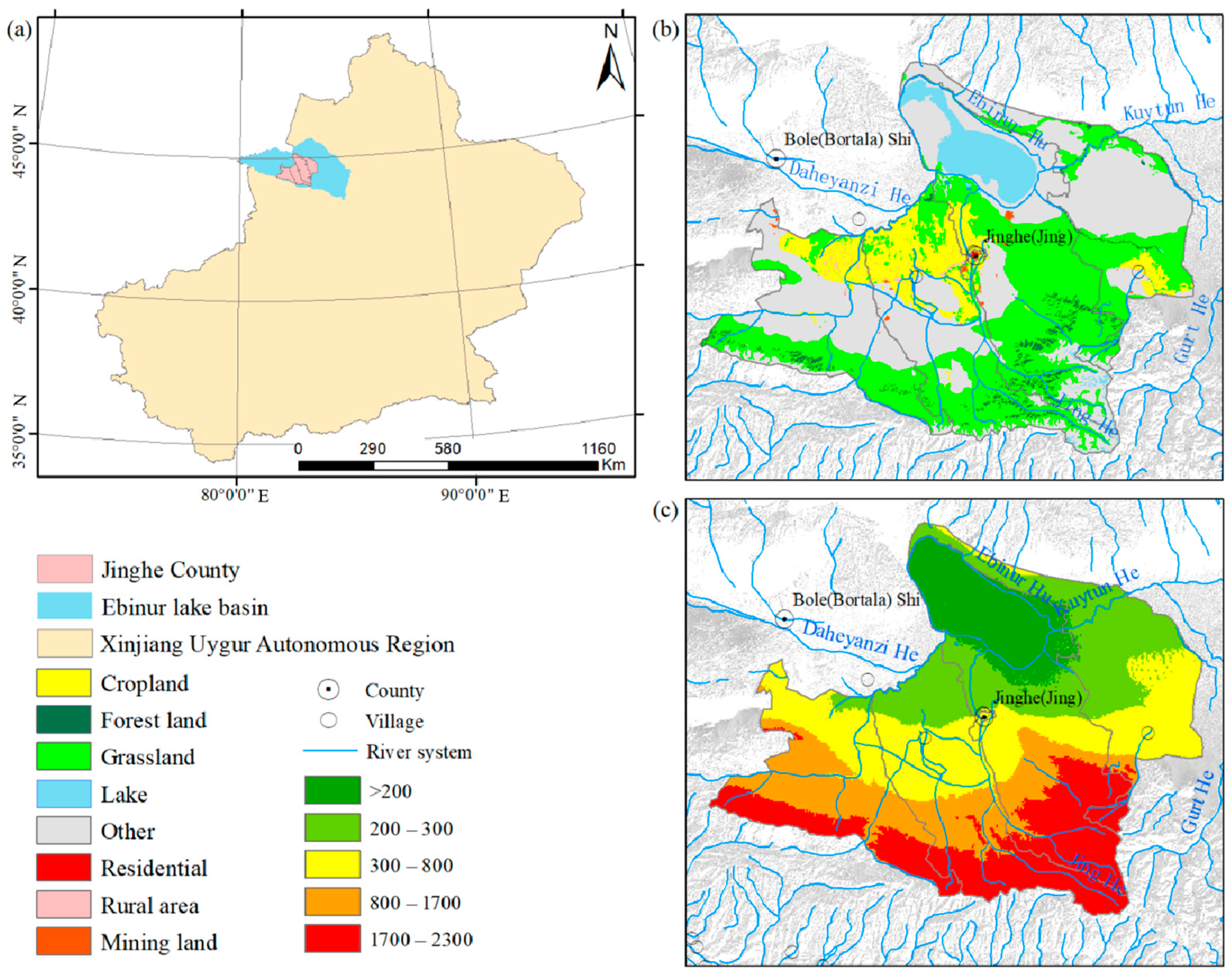
Jinghe County is located between 44°32′–45°08′ N and 82°04′–83°32′ E (as shown in Figure 1). Jinghe County in Xinjiang is located in an arid and semi-arid area and has a typical mid-temperate arid continental climate. The annual average temperature ranges from 6.6 to 7.8 °C, and the annual precipitation is between 116.0 and 169.2 mm [24]. Due to the unique topography and landforms of Xinjiang, such as the Tian Shan and Kunlun Mountains, which block the sources of moisture, rainfall is scarce. Especially in winter, the strong, dry and cold air current from the Mongolian–Siberian high-pressure area makes the climate abnormally dry and cold. Over the last four decades, Ebinur Lake has experienced a substantial decline in surface area as a result of steadily decreasing water inflows. At present, its size has diminished to under 500 km², accompanied by an overall drop in water level of 2 to 3 m [25,26]. However, the dried-up lakes have transformed into saline–alkali deserts, becoming a significant source of sand and dust weather. Due to the combined influence of various factors, the ecological environment of Jinghe County has suffered severe damage, and the balance of the ecosystem has also been significantly disrupted. Moreover, in April 2007, Ebinur Lake Wetland in Jinghe County was formally recognized as a significant ecological conservation area, owing primarily to its distinctive wetland environment and abundant biodiversity. It was officially approved as an autonomous regional-level nature reserve and a national-level nature reserve [27].

Figure 1. Overview map of the study area. (a) The location of the study area in Xinjiang Uygur Autonomous Region, (b) The distribution overview of land use and land cover in the study area in 2020. (c) Digital Elevation Map of the study area.

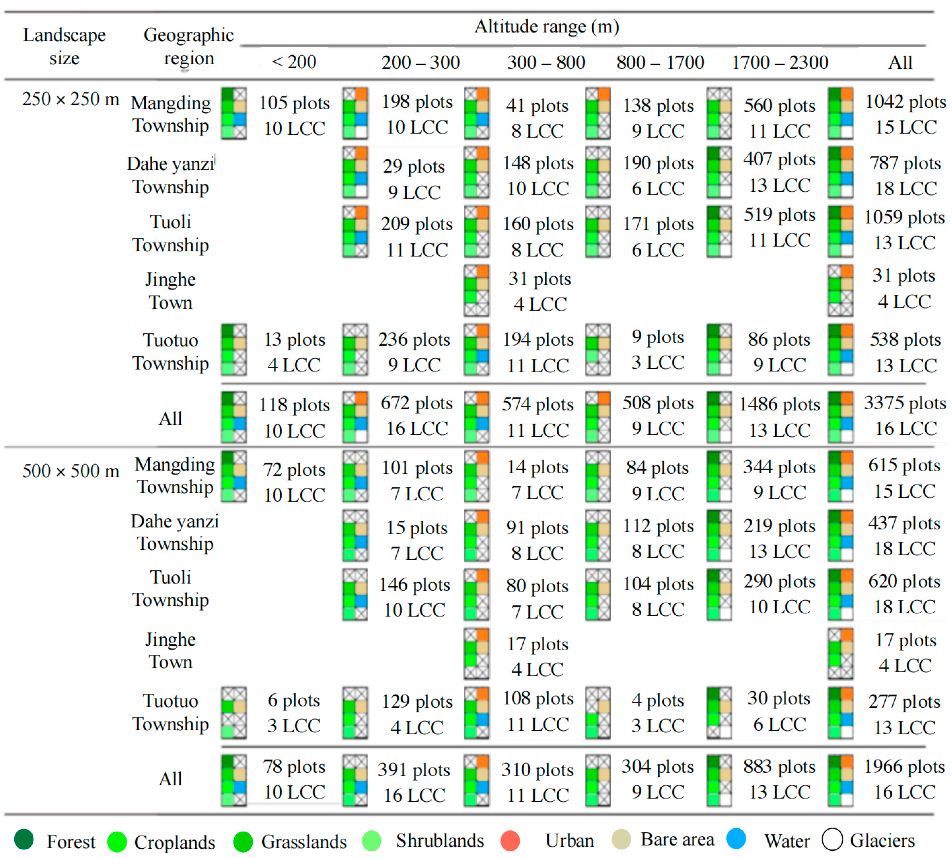
A large number of studies have shown that biodiversity has a dependence on spatial scale. To more accurately reveal the dependency characteristics of biodiversity on spatial scale, this study, based on relevant research results [28,29], set up two sampling schemes (250 × 250 m and 500 × 500 m) within the investigation area (shown Figure 2).

Figure 2. The types of land cover in different landscape sampling units under different DEM conditions (within each block, the number of land cover types was counted to reflect the gradient difference in landscape richness).

Among them, the 250 × 250 m scale can effectively capture the patch-level landscape heterogeneity of the Abi Lake wetland and meet the demand for fine description of local landscape structure; while the 500 × 500 m scale is suitable for landscape pattern analysis at the regional scale. The two together form a multi-scale comparison framework, supporting the in-depth exploration of this study on the relationship between landscape diversity and ecological function (See Figure 2).

This study adopted a sampling unit of 250 × 250 m and divided the study area into five grades based on the quantiles of altitude: <200 m, 200–300 m 300–800 m, 800–1700 m, and 1700–2300 m. The statistical results show that Jinghe County has the largest number of landscape types (a total of 16 types) within the altitude range of 200 to 300 m, the number of patches, indicating that this altitude interval has a relatively high landscape diversity. However, the number of landscape patches is the largest (reaching 1486) within the altitude range of 1700 to 2300 m, indicating a higher degree of landscape fragmentation and spatial dispersion in this area. Compared with other towns and townships, the terrain of Jinghe County’s urban area is relatively flat. Digital Elevation Model (DEM) data shows that its altitude mainly ranges from 300 to 800 m (Figure 1c). Based on the analysis of 500 × 500 m sampling units, Jinghe County has the most landscape types (a total of 16) within the altitude range of 200 to 300 m, with 391 patches. This is significantly fewer than the number of patches (672) at the 250 × 250 m sampling scale, indicating that this altitude range has a relatively high landscape diversity.

This study aims to reveal the correlation between land cover richness and landscape functions at different scales in Jinghe County, a typical county in arid areas. The specific technical route is shown in Figure 3.

Figure 3. Workflow diagram of this study.

2.2. Data Sources

2.2.1. Land Cover Dataset

The ESA-CCI–LC dataset provides annual global multi-temporal consistent land cover maps with a spatial resolution of 300 × 300 m from 1992 to 2015 [30]. This product is based on the ESA GlobCover series results and uses the GlobCover unsupervised classification process, integrating data from multiple satellite sensors, including the Medium Resolution Imaging Spectrometer (MERIS), Advanced Synthetic Aperture Radar (ASAR), Advanced Very High Resolution Radiometer (AVHRR), PROBA–V, and SPOT–VGT. According to the United Nations Food and Agriculture Organization (FAO) land cover classification standard, this dataset divides land use and land cover (LULC) into 37 categories [31,32]. The overall classification accuracy of the 2015 version map compared to the GlobCover data reaches 75.4%, providing a reliable basis for supporting climate modeling and ecological research [33].

It is technically feasible and structurally compatible to extend the ESA CCI–LC land cover dataset beyond 2015 through the “Copernicus Climate Data Store” (CDS), as many of the subsequent new-generation data products still maintain a 300 m spatial resolution and continue to use the FAO Land Cover Classification System (LCCS). However, to ensure methodological consistency and avoid introducing uncertainties, it is necessary to fully consider the differences in spectral response and observation geometry between different sensors (such as MERIS and Sentinel-3), and implement radiometric consistency corrections when necessary. Additionally, due to the differences in classification algorithm logic and temporal synthesis strategies between the old and new products, systematic reclassification and standardization processing must be carried out. The extended data sequence must undergo strict accuracy assessment and change detection to verify its spatiotemporal consistency. All preprocessing steps should be fully documented to ensure the scientific credibility and reproducibility of the extended dataset in ecological modeling and remote sensing applications [34].

The land use/cover change (LUCC) data for 2023 derived from the MODIS annual land cover product (MOD12Q1), with a resolution of 500 m. This product is based on the International Geosphere-Biosphere Programme (IGBP) classification system and employs a classification algorithm that combines decision trees with artificial neural networks, demonstrating high classification consistency and temporal sequence stability. As a widely used global land cover data source, MOD12Q1 has been extensively applied in monitoring LUCC dynamics, supporting ecosystem assessment, climate change research, and regional land management decisions, and has shown excellent application value and scientific reliability [35].

2.2.2. Climate and Climate Class Datasets

In this study, the monthly climate factor data of temperature and precipitation were all derived from the ERA5 dataset. The reanalysis precipitation data used in this study are derived from the land component product ERA5–Land of the fifth-generation global climate reanalysis dataset ERA5 developed by the European Centre for Medium-Range Weather Forecasts (ECMWF). This dataset offers high-precision precipitation estimates with a spatial resolution of 0.25° × 0.25°, integrating advanced land surface process models with multi-source observational constraints. It significantly enhances the representation of land hydrological processes, particularly excelling in soil moisture, evapotranspiration, and runoff simulation. As such, it has been widely applied in regional hydroclimatic research [36]. The quality of this dataset has been scientifically verified and demonstrated high reliability [37]. The time range of the ERA5 data covers from 2003 to 2023, with a spatial resolution of 1 × 1 km.

2.2.3. EVI Dataset

This study, among the various available MODIS products, applied the MOD13Q1 from collection 6. It is a 16-day composite product with 250 m spatial resolution that contains subproducts such as the NDVI and Enhanced Vegetation Index (EVI) among others (https://ladsweb.modaps.eosdis.nasa.gov/missions-and-measurements/products/MOD13Q1#data-availability (accessed on 8 May 2024). In this study, we selected EVI as the indicator for primary productivity. The 16-day temporal resolution of MODIS EVI products may affect the detection accuracy of the start (SOS) and end (EOS) of the growing season, especially in ecosystems with rapid vegetation dynamics. To alleviate this limitation, studies should fully recognize this limitation and adopt interpolation methods to improve the accuracy of phenological period estimation.

This research utilized the normalized vegetation index ratio approach, determining the beginning of the growing season as the day when the enhanced vegetation index initially surpassed the average of its yearly minimum and maximum levels.

This paper adopted the improved time-series algorithm (HANTS harmonic analysis method, see Oehri et al. [29]) to smooth the annual EVI time series of each study area during the vegetation growing season. This method has been widely applied in remote sensing data analysis [29]. EVI_GS was calculated through the following formula:

$${EVI}_{GS}={\int }_{SOS}^{EOS}EVI(t)dt=\overline{EVI}(EOS-SOS)$$

(1)

where $\overline{EVI}$ characterizes average growing season productivity, whereas ${EVI}_{GS}$ integrates EVI over the growing season, i.e., also factors in changes in GSL.

2.2.4. Albedo Dataset

The daily Bidirectional Reflectance Distribution Function/Albedo (BRDF/Albedo) product (MCD43) of the Moderate Resolution Imaging Spectroradiometer (MODIS) operated by the National Aeronautics and Space Administration (NASA) in version V006, with a resolution of 500 m, offers a higher daily temporal resolution compared to the previous 8-day MODIS V005 version 500 m resolution product (https://lpdaac.usgs.gov/products/mcd43a3v006/ (accessed on 8 May 2024). This improvement effectively enhances the temporal monitoring of vegetation phenology and snowmelt [38]. To maintain geometric accuracy across geographic locations, it employs a sinusoidal equal-area projection system [38]. The albedo dataset of Jinghe County adopted in this study is derived from the white space albedo data of the MOD43A3 product, with a time coverage ranging from 2003 to 2023.

2.3. Landscape Index

Different types of landscapes have varied effects on biodiversity, ecosystem balance and function, as well as the natural succession of landscape structure. In addition, different types of landscape patterns show significant differences in the ability of ecosystems to resist external disturbances. Landscape metrics analysis, as one of the core research contents of landscape ecology, can quantitatively analyze the spatial distribution pattern and morphological characteristics of various land use types, and it is an important basis for in-depth research on landscape functions and dynamic changes [39,40].

Considering the distinct characteristics of landscape patterns in arid and semi-arid regions, this research chose representative landscape metrics and utilized the spatial analysis tool Fragstats 4.2 to compute the corresponding landscape pattern indices for the study area (refer to Table 1). By integrating the analytical capabilities of Fragstats 4.2 with the calculation formulas outlined in Table 1, landscape indices for different land cover types across various elevation zones were derived.

Table 1. Descriptions of the landscape metrics chosen for this study.

Nu	Landscape Metric	Calculation Formula	The Meaning of Landscape Pattern Metrics
1	Landscape fragmention index	$C=\frac{\mathrm{N}}{\mathrm{A}}$	Landscape fragmentation serves as an indicator of how fragmented a landscape becomes, reflecting the complexity of its spatial configuration and, to some extent, the extent of human impact on landscape patterns. Increased landscape fragmentation is a major driver behind the loss of biodiversity and is strongly associated with the sustainable management and conservation of natural resources.
2	Edge Density (ED)	$\mathit{ED}=(\frac{E}{A})\times 100$	This index not only indicates the complexity of the spatial configuration within the landscape sample plots but also, to some degree, represents the stability of the overall spatial structure of the landscape pattern.
3	Landscape shape index
4	Landscape fractal dimension (PAFRAC)	$F=\frac{2}{\frac{N{\sum }_{i=1}^m{\sum }_{j=1}^n\left(\ln \left(p_{ij}\right)\times \ln \left(a_{\mathrm{ij}}\right)\right)-{\sum }_{i=1}^m{\sum }_{j=1}^n\ln \left(p_{ij}\right)\times {\sum }_{i=1}^m{\sum }_{j=1}^n\ln \left(a_{\mathrm{ij}}\right)}{N{\sum }_{i=1}^m{\sum }_{j=1}^n\ln \left(p_{ij}^2\right)-{\sum }_{i=1}^m{\sum }_{j=1}^n\ln \left(p_{ij}\right)}}$	To some extent, this indicator can represent the level of disruption that human activities impose on the landscape pattern. Theoretically, the fractal dimension values fall within the range of 1 to 2.

3. Results

3.1. Statistical Analysis of Landscape Pattern Index

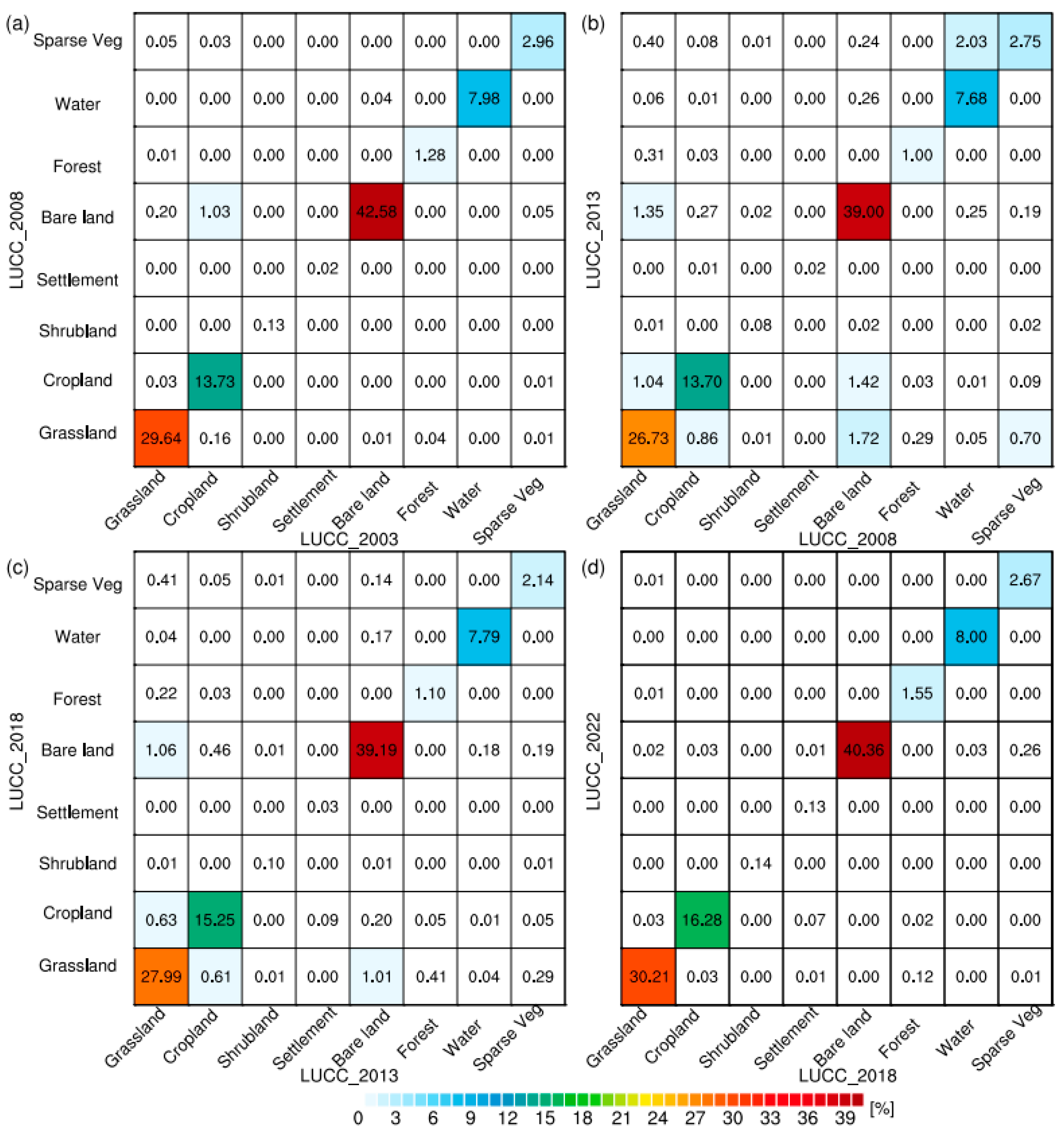
Based on the land use and land cover change (LUCC) data from 2003 to 2023, this paper analyzed the dynamic changes in the landscape pattern of the study area over the past two decades (as shown in Figure 4). The results indicated that the study area exhibited a LUCC characteristic of “dominated by bare land, large-scale conversion of grassland to cultivated land, and weak changes between water bodies and sparse vegetation”, reflecting the typical attributes of an arid/semi-arid ecologically fragile area [41]. The landscape evolution in this area was mainly influenced by human reclamation activities (such as the conversion of grassland to cultivated land) and the stability of natural landscapes (such as the stability of bare land and forest types).

Figure 4. Statistical Analysis Map of Land Use/Land Cover Changes in Jinghe County from 2003 to 2023. (a) The LUCC transfer matrix statistics chart of Jinghe County from 2003 to 2008. (b) The LUCC transfer matrix statistics chart of Jinghe County from 2008 to 2013. (c) The LUCC transfer matrix statistics chart of Jinghe County from 2013 to 2018. (d) The LUCC transfer matrix statistics chart of Jinghe County from 2018 to 2023.

During the period from 2003 to 2008, the changes in various landscape types were not significant, with only small–scale conversions between cultivated land and bare land. From 2008 to 2013, the intensity of landscape transformation significantly increased, rising notably compared to the previous period. Among them, the conversion of bare land to grassland and cultivated land was particularly prominent, with conversion areas accounting for 1.72% and 1.42% of the total area, respectively. Notably, the transformation from water bodies to sparse vegetation was the most significant, with a conversion area of 2.03% of the total area (Figure 4b). From 2013 to 2018, the overall degree of landscape transformation was relatively low, with the main changes concentrated in the mutual conversion between grassland and bare land. The areas converted from grassland to bare land and from bare land to grassland accounted for approximately 1.06% and 1.01% of the total area, respectively (Figure 4c). However, from 2018 to 2023, the landscape dynamics underwent a significant shift, with the areas of grassland, residential land, and water bodies all showing an upward trend (Figure 4d).

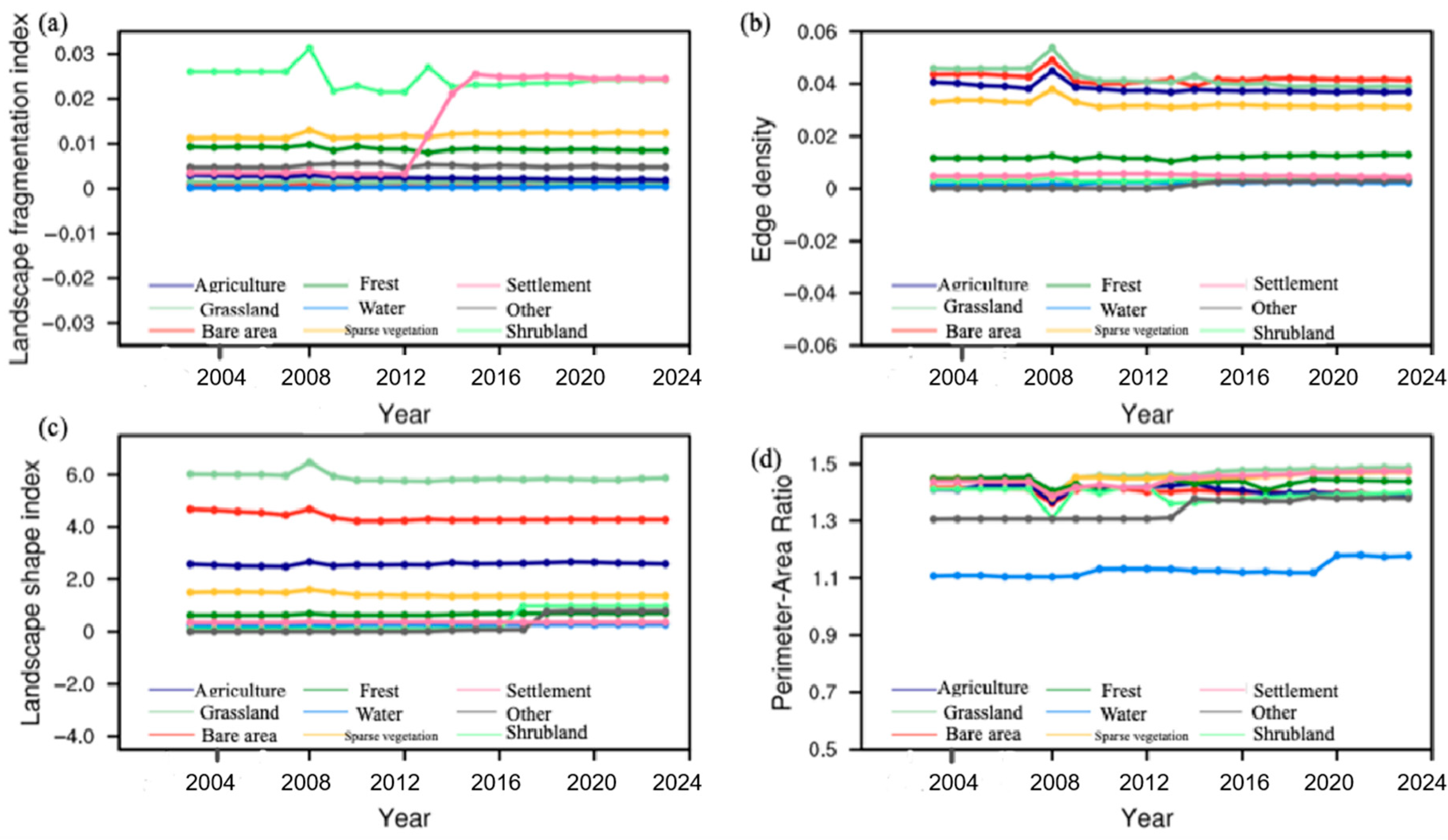
This study is based on four types of indicators, the Landscape Fragmentation index, Edge Density, landscape shape index and perimeter–area ratio, during the period from 2003 to 2023, to analyze the pattern evolution characteristics of nine types of LUCC, including Agriculture, Forest and Settlement, and further reveal the dynamic response mechanism of the landscape ecosystem. (Shown Figure 5).

Figure 5. Interannual variation trend map in Landscape Pattern Indices in Jinghe County from 2003 to 2023. (a) Landscape fragmentation Index in Jinghe County from 2003 to 2023. (b) Landscape Edge density in Jinghe County from 2003 to 2023. (c) Landscape shape Index in Jinghe County from 2003 to 2023. (d) Landscape Perimeter-area ratio Index in Jinghe County from 2003 to 2023.

During the period from 2003 to 2023, the fragmentation indices of different landscape types showed interannual variations (Shown Figure 5). The Landscape fragmentation of Forest land fluctuated significantly. It reached its peak from 2006 to 2008 due to factors such as logging and fires. After ecological restoration, it gradually declined, reflecting the process of recovery of forest patch connectivity. Settlements remained stable before 2012. From 2012 to 2023, they tended to disperse due to urban expansion, and the fragmentation index continued to rise, indicating that human activities have intensified the disturbance to land resources. From 2003 to 2023, the marginalization indices of water bodies, shrublands, forestlands and residential areas remained stable over the long term, with low marginal densities and little change, indicating that they interacted little with their surroundings and experienced minor changes in marginal morphology when disturbed, thus having weak marginal effects. In contrast, the indices of other land types were higher and fluctuated between 2012 and 2016. The landscape shape index shows significant differences among different land types.

3.2. Primary Productivity and Phenology

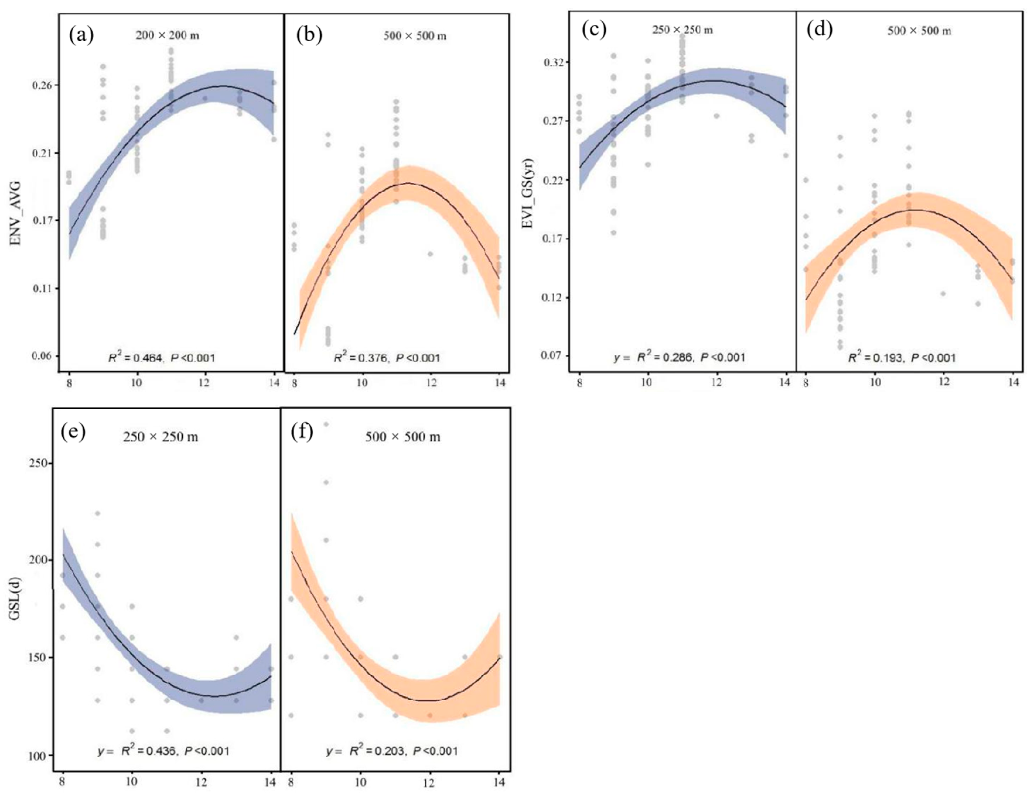
This paper selected one of the main productivity indicators: the enhanced vegetation index (EVI). EVI reflects the productivity during the average growing season, while EVI_GS represents the comprehensive change in EVI within the growing season, reflecting the dynamic changes in the growing season length (GSL). This study investigates the relationship between land cover diversity and landscape functionality in Jinghe County (Shown Figure 6), with the objective of uncovering their interactive effects on the development of spatial configurations.

Figure 6. Effects of landscape richness on landscape functioning variables. (a) Correlation between landscape diversity and the enhanced vegetation index (EVI_AVG) in a 250 × 250 m sampling area (b) Correlation between landscape diversity and the enhanced vegetation index (EVI_AVG) in a 500 × 500 m sampling area (c) Correlation between landscape diversity and the comprehensive change in EVI within the growing season (ESV_GS) in a 250 × 250 m sampling area (d) Correlation between landscape diversity and the comprehensive change in EVI within the growing season (ESV_GS) in a 500 × 500 m sampling area (e) Correlation between landscape diversity and the dynamic changes in the growing season length (GSL) in a 250 × 250 m sampling area (f) Correlation between landscape diversity and the dynamic changes in the growing season length (GSL) in a 500 × 500 m sampling area.

The differences in the correlation between landscape diversity and the Enhanced Vegetation Index (EVI_AVG, reflecting vegetation coverage and vitality) at two resolutions of 250 × 250 m (left, blue fit) and 500 × 500 m (right, orange fit) were compared, aiming to explore how scale affects their relationship. The results indicated that within a 200 × 200 m sampling area, the goodness of fit R² was higher at the 250 × 250 m resolution (0.464 > 0.376), suggesting that at this scale, landscape diversity has a stronger explanatory power for EVI_AVG, meaning that the relationship between land type diversity and vegetation vitality is more closely related (Shown Figure 6a,b). It is precisely because high resolution more accurately matches the “true pattern of landscape diversity” with the “spatial distribution of vegetation vitality reflected by EVI_AVG”, and reduces the interference of “heterogeneity integration” on the correlation signal under low resolution, which conforms to the core view of the scale dependence theory that “there exists an ‘optimal resolution threshold’ for specific ecological relationships”.

Figure 6c shows the nonlinear relationship between landscape richness and the comprehensive growth productivity (GSI) at two spatial resolutions of 250 × 250 m and 500 × 500 m: when the richness is low, GSI decreases as it increases, due to the fragmentation of dominant land types causing damage to vegetation connectivity; when the richness is high, GSI increases as it increases, as a result of the complementarity of land types promoting ecological processes. It reveals that the nonlinear correlation between the two is highly dependent on the spatial resolution, and a smaller scale can more accurately depict the impact of land type diversity on ecosystem productivity.

This paper further analyzed the influence of landscape richness (represented by log (LR) on ecosystem productivity and phenology under different landscape functions and scales. The results are presented in Table 2. At a small scale of 250 × 250 m, the average linear effect of log(LR) on NE was $0.0453 \pm 0.01$ ($F_{\mathrm{1,18}}=6.1, p<0.001$), and the positive effect of NE was $0.227 \pm 0.004$($t_{19}$, p < 0.001). According to the scale-dependent theory, landscape heterogeneity at a small scale mainly manifests as “local microhabitat differences”, such as edge effects of vegetation patches or small-scale disturbances of bare land. Although the landscape richness reflected by log(LR) can explain the changes in NE, the fragmented characteristics of the small-scale pattern limit the association strength from reaching the optimal state. For instance, the sporadic distribution of grassland patches may mask the overall regulatory effect of land type diversity on ecosystem productivity, resulting in both the linear effect and the positive effect of NE being at a moderate level. At a medium scale of 500 × 500 m, the linear effect of log(LR) rose to $0.711 \pm 0.02$, and the positive effect of NE increased to $0.357 \pm 0.007$, with a smaller p value in the statistical test, showing a trend of “scale amplification, association enhancement”. This result is in line with the “pattern integration effect” in the scale-dependent theory: at a medium scale, the random disturbances of local microhabitats are weakened, and log(LR) can more effectively capture the macroscopic combination patterns of different land types (such as the contiguous distribution of grassland, water bodies, and cultivated land). Such macroscopic patterns have a more stable regulatory effect on ecosystem productivity (EVI_AVG), for example, the water supply of water bodies to surrounding vegetation and the complementary material cycle between cultivated land and grassland. As a result, the association between log(LR) and NE is significantly enhanced, further supporting the theoretical viewpoint that “specific ecological relationships have an optimal scale threshold”. Secondly, in terms of the EVI_GS function, at the 250 × 250 scale, the positive effect of NE was 0.281 ± 0.004 (t₃₅ = 6.0, p < 0.001), and the linear effect of log (LR) was 0.085 ± 0.008 (F₁,₁₇ = 5.9, p < 0.001). Although the mean of the linear effect of log (LR) was lower than that of EVI_AGV, it still reached a significant level, indicating that the influence mechanisms of different ecological functions (AGV, GS) on NE are different. At the 500 × 500 scale, the positive effect of NE was 0.325 ± 0.004 (t₁₆ = 4.0, p = 0.030), and the linear effect of log (LR) was 0.113 ± 0.0201 (F_1,15 = 5.9, p < 0.001). As the scale increased, the positive effect of NE strengthened, and its correlation with the landscape pattern became more significant. However, compared with EVI_AGV, the mean of NE for EVI_GS was relatively lower, further reflecting the differences in the driving mechanisms of different vegetation functions on the NE of ecosystem productivity. Unlike productivity and growing season functions, EVI_GSL shows the characteristics of “scale amplification, weakened positive effect of NE, and high dispersion”: at the 250 m scale, the positive effect of NE is $3.652 \pm 3.18 (p < 0.001)$; while at the 500 m scale, this effect drops to $1.172 \pm 2.92 (p = 0.03)$ and the standard error remains relatively large. According to the scale-dependent theory, phenological processes (such as the green-up and senescence periods of vegetation) are more susceptible to small-scale factors like “microtopography” and “local microclimate”. At small scales, local warming effects (such as heat accumulation in low-lying areas) may significantly advance phenological periods; however, at medium scales, such local signals are often masked or counteracted by macroscopic climate at the regional scale (such as large-scale cooling), leading to an unstable relationship between log(LR) and NE. This “fragmented” association reflects the highly context-dependent response of phenology to landscape patterns, confirming the theoretical characteristic that “phenological dynamics are more dependent on micro-scale ecological processes and are more vulnerable to external climate disturbances at macro scales”.

Table 2. The influence of the net effect (NE) of diversity in different scale landscape sampling areas on ecosystem productivity and vegetation phenology.

Category	Landscape Function Index	Scale of Landscape Sampling Area	NE > 0 Effect (Mean ± s.e.m.) a	NE > 0 Effect Significance (One-Sample t-Test) a	Linear Effect of Log(LR) on NE (Mean ± s.e.m.) a	Linear Effect of Log(LR) on NE Significance (F-Test) a
Productivity	EVI_AGV	250 × 250	0.227 ± 0.004	t19 = 6.0; p < 0.001	0.453 ± 0.015	F1,18 = 6.1; p < 0.001
		500 × 500	0.357 ± 0.007	t16 = 2.0; p = 0.04	0.711 ± 0.024	F1,15 = 3.2; p < 0.001
	EVI_GS	250 × 250	0.281 ± 0.004	t35 = 6.0; p < 0.001	0.085 ± 0.008	F1,17 = 5.9; p < 0.001
		500 × 500	0.325 ± 0.004	t16 = 4.0; p = 0.030	0.113 ± 0.0201	F1,15 = 5.9; p < 0.001
Phenology	EVI_GSL	250 × 250	3.652 ± 3.18	t18 = 6.0; p < 0.001	5.127 ± 5.621	F1,17 = 5.9; p < 0.001
		500 × 500	1.172 ± 2.92	t16 = 4.0; p < 0.030	3.172 ± 2.932	F1,21 = 1.53; p < 0.001

“a” represents the Mean ± the standard error of mean.

In this paper, we set up two plots containing landscapes, with grid spaces of 250 × 250 m or 500 × 500 m. We also incorporated relevant covariates to include terrain, climate and land cover conditions in our model (Table 2), but similar to BGR and altitude, the impact of biodiversity remained significant even when these conditions were similar.

The results of this study on the impact of landscape richness on landscape functional variables differ from those of Oehri et al. [28,29]. The main reason lies in the fact that the growing season of vegetation in arid areas is relatively short and strictly limited by water conditions, which leads to essential differences in phenological dynamics and productivity response mechanisms compared to forests in humid or temperate regions. Additionally, the dominant bare land and large-scale conversion of grassland to farmland in the study area further complicate the relationship between landscape patterns and ecological processes, making the influence path of landscape richness on functional variables more environmentally dependent.

3.3. Correlation Between Landscape Indicators and Ecosystem Functions at Different Scales

This paper analyzes the pairwise correlation between landscape pattern indices (such as EVL_GSL, PD, etc.) and environmental factors (such as Precip, Temp, etc.) to explore the relationship between landscape patterns and environmental variables (Figure 7).

Figure 7. The correlation analysis among landscape diversity, environmental covariates, and landscape functional variables across different spatial scales of landscape plots (250 × 250 m and 500 × 500 m). (a) Correlation analysis of landscape diversity, environmental covariates and landscape functional variables at the 250 × 250 m landscape plot spatial scale (b) Correlation analysis of landscape diversity, environmental covariates and landscape functional variables at the 500 × 500 m landscape plot spatial scale.

For the 250 × 250 m scale, the synergy and coupling of landscape pattern indices: PD (patch density), AI (aggregation index) and slope show a large number of deep blue squares, indicating a strong positive correlation. The essence lies in the “precise regulation of patch structure by local terrain micro-features” at a small scale. Environmental factors: precipitation, temperature, EVI_AVG, EVI_GS and other environmental variables show a significant negative correlation. This is due to the “dynamic balance of local micro-environmental heterogeneity” at a small scale. Within the 250 × 250 m range, it precisely depicts the local feedback mechanism between “microclimate and vegetation” at a small scale, confirming the assertion in the scale-dependent theory that “environmental factor correlations at a small scale highlight micro-domain differences”. Local driving of landscape pattern and environment: The dark squares between EVI_GSL (growing season length) and temperature indicate a strong correlation, which is caused by the “direct impact of local temperature micro-differences on phenology” at a 250 × 250 m scale.

At the 500 × 500 m scale, the landscape pattern indices exhibit significant internal integration characteristics: ED (edge density), PD (patch density), and FRA (fractal dimension) show a significant positive correlation. This phenomenon reflects the “macroscopic landscape heterogeneity’s integration and regulation of multi-dimensional patterns” mechanism at a large scale. In terms of environmental factors, a deep red square appears between temperature (Temp) and COHESION (connectivity index), indicating a strong negative correlation, which reflects the “macroscopic regulation of landscape structure by regional climate” at a large scale. Within the 500 × 500 m range, climate change affects the growth status of vegetation and thereby alters landscape connectivity, forming a systematic environmental-structural response relationship, supporting the judgment in the scale-dependent theory that “large-scale environmental factors’ associations reflect macroscopic constraints”. The macroscopic response between landscape patterns and the environment is manifested in a certain degree of correlation between EVI_GSL and Precip (precipitation), the cause of which lies in the “overall driving of regional precipitation patterns on phenology” at the 500 m scale, that is, the spatial distribution pattern of precipitation has a systematic impact on the length of the vegetation growing season.

The sampling scale has a significant impact on the representation of landscape patterns. The small-scale sampling of 250 × 250 m can reflect local features, such as patch shape and edge structure, more precisely. Therefore, the correlation of landscape pattern indices in Figure 7a is more obvious at the local level. In contrast, the large-scale sampling of 500 × 250 m integrates local details and focuses on reflecting the overall pattern. The correlation in Figure 7b is more inclined to the overall characteristics.

In terms of environmental factors, the landscape pattern at a small scale is more directly influenced by the local micro-environment. The correlation in Figure 7a better reflects the effect of the local environment on the landscape. At a large scale, it mainly reflects the association between the regional environment and the overall landscape pattern, as shown in Figure 7b.

Furthermore, changes in scale may affect the representation of landscape pattern indices and environmental factors, thereby altering the magnitude and significance of correlation coefficients. For instance, some significant correlations at a small scale may no longer be significant at a large scale, or the degree of correlation may change.

3.4. Relative Importance of Landscape Richness Effects

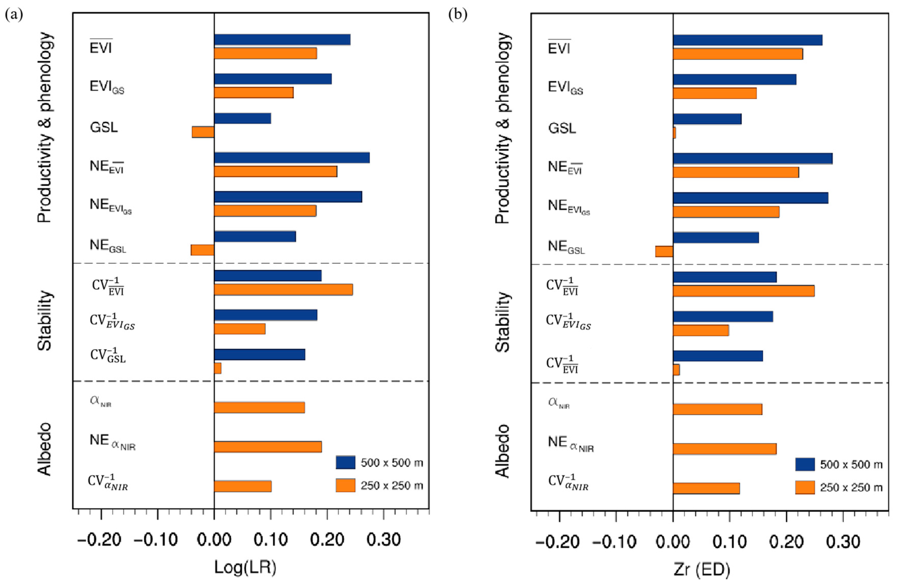
We calculated the normalized effect size based on the correlation coefficient (Zr; Fisher’s Z-transform) to quantify the relative importance of logarithms (LR) for all dependent variables (Figure 8).

Figure 8. Normalized effect sizes (Zr) of landscape richness for all landscape. (a) Zr values are shown for Log(LR): log-transformed landscape richness (b) Zr values are shown for ED: log(LR): log-transformed landscape richness.

At a small scale of 250 × 250 m, the ecological effect is characterized by “low Zr values and high stability fluctuations” dominated by local micro-fluctuations. Regarding the Zr values: the Zr value range of log(LR) is 0.1 to 0.23, and that of ED is 0.15 to 0.25, both in relatively low intervals; the Zr value of species richness effect is 0.17, also at a low level. In terms of stability indicators: the values of CV⁻¹ enhanced vegetation index and EVI_GS are between 0 and 0.25, with small fluctuation amplitudes but high frequencies, reflecting frequent local environmental dynamic changes.

At the large scale of 500 × 500 m, the ecological effects exhibit a characteristic of “high Zr value and low stability fluctuation” dominated by macroscopic overall stability. Regarding the Zr value: the Zr values of log(LR) and ED still fall within the range of 0.1 to 0.25, but the Zr value of the species richness effect rises to 0.21, an increase of approximately 23.5% compared to the 250 m scale, indicating that the biodiversity effect is more significant at a larger scale. In terms of stability indicators: CV⁻¹ enhanced vegetation index and EVI_GS remain within the range of 0 to 0.25, but the frequency of fluctuations has significantly decreased, demonstrating a stronger overall stability.

The Zr value of species richness effect at the 250 × 250 m scale (0.17) is lower than that at the 500 × 500 m scale (0.21), reflecting the “scale threshold effect of species richness—functional association” in the theory—at a smaller scale, species richness is more susceptible to local disturbances (such as patch fragmentation), and the complementary effect is difficult to fully exert, resulting in a lower regulatory intensity of productivity (Zr value); at a larger scale, species richness is more stable due to the support of the macro-environment. The stability indicators (CV⁻¹ enhanced vegetation index, EVI_GS) are between 0 and 0.25, indicating that the fluctuation range of productivity indicators is small, reflecting the “synergistic support of landscape richness and species richness for functional stability”.

The large scale of 500 × 500 m integrates more landscape and environmental information, and for indicators reflecting the overall pattern (such as productivity and phenological indicators), the correlation amplitude (Log (LR) or Zr (ED) values) with related elements is stronger; while the small scale of 250 × 250 m focuses more on local features, and the correlation with indicators reflecting local differences (such as stability and albedo-related indicators) is more obvious. Scale changes can affect the manifestation of ecological processes. For example, GSL and NE_GSL show a weak negative correlation at the small scale but turn to a positive correlation at the large scale, indicating that scale has a regulatory effect on the correlation direction and significance, reflecting the spatial heterogeneity of the ecosystem.

Smaller scales are more capable of capturing local ecological processes (such as vegetation phenology and albedo fluctuations), and the correlations of their indicators with the environment reflect local mechanisms; larger scales, on the other hand, better represent regional ecological patterns (such as productivity distribution), and their correlations reflect overall laws. Combining both scales helps to comprehensively understand the multi-scale characteristics of ecological processes.

4. Conclusions and Discussion

4.1. Conclusions

To investigate the relationship between landscape diversity and ecosystem function in a structured manner, this study developed a core evaluation framework. This framework utilized the Enhanced Vegetation Index (EVI), derived from satellite remote sensing data, as a key measure of primary productivity. Additionally, average growth productivity—encompassing both EVI and overall growth performance—was incorporated as a complementary metric reflecting vegetation productivity and phenological patterns. Based on this framework, multi-scale landscape plots were designed, and a comprehensive analysis was conducted using time-series remote sensing data. The main research results are as follows:

• The landscape pattern changes in the study area over the past two decades have shown phased characteristics. From 2003 to 2008 and from 2013 to 2018, landscape transformation was relatively weak. From 2008 to 2013, transformation intensified, with a significant shift from water bodies to sparse vegetation. From 2018 to 2023, the areas of grassland, residential land, and water bodies have increased. These changes reflect the dynamic responses of the landscape ecosystem under the combined influence of natural disturbances, ecological restoration, and human activities.
• Landscape diversity has a stronger explanatory power for EVI_AVG at a resolution of 250 × 250 m. Under different landscape functions and scales, the impact of log (LR) on ecosystem productivity and phenological indicators shows significant differences. Generally speaking, as the spatial scale increases, the positive effect of NE strengthens and its association with landscape patterns becomes more intimate. However, the response of NE related to phenology to landscape patterns is more complex, with its mean value decreasing as the scale increases.
• At the sampling scales of 250 × 250 m and 500 × 500 m, there are varying degrees of correlations among landscape pattern indices, environmental factors, and between the two. The smaller scale more accurately reflects the local features and the influence of micro-environment on the landscape, while the larger scale focuses on the overall pattern and the general association between the regional environment and the landscape. Scale changes influence both the direction and significance of ecological correction
• Under the two landscape plot scales of 250 × 250 m and 500 × 500 m, the overall direction of ecological effects is consistent, but certain differences are manifested. Meanwhile, scale changes can regulate the direction and significance level of the correlation of ecological processes. Combining the analysis of the two scales helps to understand the multi-scale characteristics of ecological processes at different spatial levels more comprehensively.

4.2. Discussion

This study still has some shortcomings. On the one hand, it is necessary to deeply reveal the mechanism of the impact of landscape richness on the ecological environment. Not only should the internal driving path and ecological feedback process be clarified, but the dynamic relationship between habitat productivity, potential soil coverage and biodiversity should also be focused on. These three factors are significantly positively correlated in the ecosystem, but the current study has not fully combined this correlation rule to analyze the ecological effect of landscape richness. At the same time, the existing research has not clearly defined how the landscape richness-related indicators (such as landscape diversity index, patch structure index) consider the deformed influence of key environmental factors such as soil pH value (affecting vegetation growth efficiency and thus changing habitat productivity) and humus content (determining soil fertility and structure and affecting the stability of potential soil coverage). This leads to the mechanism analysis not fully covering the interaction between key elements of the ecosystem, thereby weakening the systematic understanding of the ecological value of landscape richness. On the other hand, human activity factors should be systematically incorporated into the landscape pattern analysis framework. By integrating key variables such as land use intensity, urban–rural development pressure and management policies, the scientificity and comprehensive explanatory power of the research in explaining ecosystem response can be enhanced [42,43].

References

- Nepali, B.R.; Skartveit, J.; Baniya, C.B. Impacts of slope aspects on altitudinal species richness and species composition of Narapani-Masina landscape, Arghakhanchi, West Nepal. J. Asia-Pac. Biodivers. 2021, 14, 415–424. [Google Scholar] [CrossRef]
- Santos, J.P.; Sobral-Souza, T.; Brown, K.S., Jr.; Vancine, M.H.; Ribeiro, M.C.; Freitas, A.V. Effects of landscape modifi-cation on species richness patterns of fruit-feeding butterflies in Brazilian Atlantic Forest. Divers. Distrib. 2020, 26, 196–208. [Google Scholar] [CrossRef]
- Rodríguez, S.L.; van Bussel, L.G.; Alkemade, R. Classification of agricultural land management systems for global modeling of biodiversity and ecosystem services. Agric. Ecosyst. Environ. 2024, 360, 108795. [Google Scholar] [CrossRef]
- Sahle, M.; Yeshitela, K. Dynamics of land use land cover and their drivers study for management of ecosystems in the socio-ecological landscape of Gurage Mountains, Ethiopia. Remote Sens. Appl. Soc. Environ. 2018, 12, 48–56. [Google Scholar] [CrossRef]
- Wang, Q.; Wang, H. Spatiotemporal dynamics and evolution relationships between land-use/land cover change and landscape pattern in response to rapid urban sprawl process: A case study in Wuhan, China. Ecol. Eng. 2022, 182, 106716. [Google Scholar] [CrossRef]
- Mendoza-Ponce, A.; Corona-Núñez, R.; Kraxner, F.; Leduc, S.; Patrizio, P. Identifying effects of land use cover changes and climate change on terrestrial ecosystems and carbon stocks in Mexico. Glob. Environ. Change 2018, 53, 12–23. [Google Scholar] [CrossRef]
- Le Provost, G.; Thiele, J.; Westphal, C.; Penone, C.; Allan, E.; Neyret, M.; van der Plas, F.; Ayasse, M.; Bardgett, R.D.; Birkhofer, K.; et al. Contrasting responses of above- and belowground diversity to multiple components of land-use intensity. Nat. Commun. 2021, 12, 3918. [Google Scholar] [CrossRef] [PubMed]
- Tammaru, T.; Valdma, D.; Tiitsaar, A.; Kaasik, A.; Õunap, E.; Remm, J.; Teder, T. Landscape-level determinants of butterfly species richness in northern Europe: A country-wide survey reveals the paramount importance of forest land. Biol. Conserv. 2023, 286, 110294. [Google Scholar] [CrossRef]
- Dem, P.; Hayashi, K.; Fujii, M.; Mohmmed, E.E.E. Integrating biodiversity and ecosystem services in land use change assessment through sustainability indicator. Environ. Impact Assess. Rev. 2025, 114, 107971. [Google Scholar] [CrossRef]
- Sõber, V.; Leps, M.; Kaasik, A.; Mänd, M.; Teder, T. Forest proximity supports bumblebee species richness and abundance in hemi-boreal agricultural landscape. Agric. Ecosyst. Environ. 2020, 298, 106961. [Google Scholar] [CrossRef]
- van Strien, M.J.; Slager, C.T.; De Vries, B.; Grêt-Regamey, A. An improved neutral landscape model for recreating real landscapes and generating landscape series for spatial ecological simulations. Ecol. Evol. 2016, 6, 3808–3821. [Google Scholar] [CrossRef]
- Oita, S.; Ibáñez, A.; Lutzoni, F.; Miadlikowska, J.; Geml, J.; Lewis, L.A.; Hom, E.F.Y.; Carbone, I.; U’Ren, J.M.; Arnold, A.E. Climate and seasonality drive the richness and composition of tropical fungal endophytes at a landscape scale. Commun. Biol. 2021, 4, 313. [Google Scholar] [CrossRef]
- Bellón, B.; Henry, D.A.; Renaud, P.-C.; Roque, F.d.O.; Santos, C.C.; Melo, I.; Arvor, D.; de Vos, A. Landscape drivers of mammal habitat use and richness in a protected area and its surrounding agricultural lands. Agric. Ecosyst. Environ. 2022, 334, 107989. [Google Scholar] [CrossRef]
- Zimbres, B.; Peres, C.A.; Machado, R.B. Terrestrial mammal responses to habitat structure and quality of remnant riparian forests in an Amazonian cattle-ranching landscape. Biol. Conserv. 2017, 206, 283–292. [Google Scholar] [CrossRef]
- Mu, T.; Zhao, R.; Li, H.; Lei, Y.; Chen, Q.; Tian, G.; Zhang, Y.; Mu, B. A Novel Indicator for Assessing Spatial Coupling Relationships within Hybrid Landscapes Comprising Diverse Land Cover Types and Its Application to Explaining Urban Thermal Environment. Sustain. Cities Soc. 2025, 130, 106595, Correction in Sustain. Cities Soc. 2025, 132, 106828. [Google Scholar] [CrossRef]
- Cui, Y.; Zhao, C.; Pan, Y.; Ma, K.; Liu, X.; Gu, X. Decoding spatial consistency of multi-Source land cover products in China: Insights from heterogeneous landscapes. Int. J. Appl. Earth Obs. Geoinf. 2025, 139, 104529. [Google Scholar] [CrossRef]
- Coelho, A.J.P.; Teixeira, H.M.; Verweij, P.; Matos, F.A.R.; Villa, P.M.; Meira-Neto, J.A.A. Functional richness mediates landscape and management effects on tree biomass and soil fertility during secondary forest succession. Ecol. Indic. 2024, 162, 112029. [Google Scholar] [CrossRef]
- Gong, J.; Jin, T.; Cao, E.; Wang, S.; Yan, L. Is ecological vulnerability assessment based on the VSD model and AHP-Entropy method useful for loessial forest landscape protection and adaptative management? A case study of Ziwuling Mountain Region, China. Ecol. Indic. 2022, 143, 109379. [Google Scholar] [CrossRef]
- Risal, A.; Karki, R.; Qi, J. Integrating remote sensing data with watershed-scale ecohydrological modeling in diverse forest and agricultural landscapes of the Upper Mississippi River Basin. Environ. Model. Softw. 2025, 192, 106588. [Google Scholar] [CrossRef]
- Zhang, Y. Quantitative analysis of surface landscape elements for landscape environmental design—Based on high resolution remote sensing image technology. Syst. Soft Comput. 2025, 7, 200325. [Google Scholar] [CrossRef]
- Guo, J.; Huang, W.; Dong, Y.; Lin, K.; Yue, F.; Shan, Y.; Liu, H.; Hao, Z.; Wang, N.; Ding, X. A weight-adaptive updated method for grasshopper habitat mapping at the national scale using remote sensing: Combined with spatial heterogeneity and landscape. ISPRS J. Photogramm. Remote Sens. 2025, 227, 84–98. [Google Scholar] [CrossRef]
- Cheng, S.; Yang, X.; Yang, G.; Chen, B.; Chen, D.; Wang, J.; Ren, K.; Sun, W. Using ZY1-02D satellite hyperspectral remote sensing to monitor landscape diversity and its spatial scaling change in the Yellow River Estuary. Int. J. Appl. Earth Obs. Geoinf. 2024, 128, 103716. [Google Scholar] [CrossRef]
- Halder, S.; Bose, S. Remote sensing insights for sustainable development: Water quality and landscape dynamics in Mirik Lake, Darjeeling District, West Bengal, India. Clean. Water 2024, 2, 100024. [Google Scholar] [CrossRef]
- Ren, Y.; Zhang, F.; Kung, H.-T.; Johnson, V.C.; Wang, J.; Zhang, Y.; Yu, H.; Yushanjiang, A. Using the vegetation-solar radiation (VSr) model to estimate the short-term gross primary production (GPP) of vegetation in Jinghe county, XinJiang, China. Ecol. Eng. 2017, 107, 208–215. [Google Scholar] [CrossRef]
- Wang, Z.; Zhang, X.; Zhang, F.; Chan, N.W.; Kung, H.-T.; Liu, S.; Deng, L. Estimation of soil salt content using machine learning techniques based on remote-sensing fractional derivatives, a case study in the Ebinur Lake Wetland National Nature Reserve, Northwest China. Ecol. Indic. 2020, 119, 106869. [Google Scholar] [CrossRef]
- Lin, Q.; Xu, W. Analysis of the effect of the quantity of inflow into Ebinur Lake on its ecological security. Environ. Res. 2025, 266, 120517. [Google Scholar]
- Zhang, F.; Yushanjiang, A.; Jing, Y. Assessing and predicting changes of the ecosystem service values based on land use/cover change in Ebinur Lake Wetland National Nature Reserve, Xinjiang, China. Sci. Total. Environ. 2019, 656, 1133–1144. [Google Scholar] [CrossRef] [PubMed]
- Oehri, J.; Bürgin, M.; Schmid, B.; Niklaus, P.A. Local and landscape-level diversity effects on forest functioning. PLoS ONE 2020, 15, e0233104. [Google Scholar] [CrossRef] [PubMed]
- Oehri, J.; Schmid, B.; Schaepman-Strub, G.; Niklaus, P.A. Terrestrial land-cover type richness is positively linked to landscape-level functioning. Nat. Commun. 2020, 11, 154. [Google Scholar] [CrossRef]
- Habibie, M.I.; Nurda, N.; Fernando, D.; Arifandri, R.; Putra, P.K.; Prayogi, H.; Sencaki, D.B. Integrating Sentinel-2 and ESA world cover for effective land use and land cover assessment using machine learning. Adv. Space Res. 2025, 76, 4925–4958. [Google Scholar] [CrossRef]
- Mousivand, A.; Arsanjani, J.J. Insights on the historical and emerging global land cover changes: The case of ESA-CCI-LC datasets. Appl. Geogr. 2019, 106, 82–92. [Google Scholar] [CrossRef]
- Reinhart, V.; Fonte, C.; Hoffmann, P.; Bechtel, B.; Rechid, D.; Boehner, J. Comparison of ESA climate change initiative land cover to CORINE land cover over Eastern Europe and the Baltic States from a regional climate modeling perspective. Int. J. Appl. Earth Obs. Geoinf. 2021, 94, 102221. [Google Scholar] [CrossRef]
- Tan, M.L.; Tew, Y.L.; Chun, K.P.; Samat, N.; Shaharudin, S.M.; Mahamud, M.A.; Tangang, F.T. Improvement of the ESA CCI Land cover maps for water balance analysis in tropical regions: A case study in the Muda River Basin, Malaysia. J. Hydrol. Reg. Stud. 2021, 36, 100837. [Google Scholar] [CrossRef]
- Copernicus Climate Change Service, Climate Data Store. Land Cover Classification Gridded Maps from 1992 to Present Derived from Satellite Observation; Copernicus Climate Change Service (C3S) Climate Data Store (CDS). 2019. Available online: https://cds.climate.copernicus.eu/datasets/satellite-land-cover?tab=download (accessed on 8 May 2024).
- Sun, L.; Wei, J.; Duan, D.; Guo, Y.; Yang, D.; Jia, C.; Mi, X. Impact of Land-Use and Land-Cover Change on urban air quality in representative cities of China. J. Atmos. Sol.-Terr. Phys. 2016, 142, 43–54. [Google Scholar] [CrossRef]
- Lan, G.; Liang, Y.; Ma, Y. Assessment of precipitation reanalysis product ERA5 on summer extreme precipitation in the Yellow River Basin. Dyn. Atmos. Oceans 2025, 112, 101603. [Google Scholar] [CrossRef]
- Ding, A.; Liang, S.; Ma, H.; He, T.; Jia, A.; Wang, Q. Improved estimation of daily blue-sky snow shortwave albedo from MODIS data and reanalysis information. Sci. Remote Sens. 2024, 10, 100163. [Google Scholar] [CrossRef]
- Peng, S.; Ding, Y.; Liu, W.; Li, Z. 1 km monthly temperature and precipitation dataset for China from 1901 to 2017. Earth Syst. Sci. Data 2019, 11, 1931–1946. [Google Scholar] [CrossRef]
- Riitters, K.; Vogt, P. Mapping landscape ecological patterns using numeric and categorical maps. PLoS ONE 2023, 18, e0291697. [Google Scholar] [CrossRef]
- Hersperger, A.M.; Grădinaru, S.R.; Daunt, A.B.P.; Imhof, C.S.; Fan, P. Landscape ecological concepts in planning: Review of recent developments. Landsc. Ecol. 2021, 36, 2329–2345. [Google Scholar] [CrossRef]
- Zhang, Y.; Tariq, A.; Hughes, A.C.; Hong, D.; Wei, F.; Sun, H.; Sardans, J.; Peñuelas, J.; Perry, G.; Qiao, J.; et al. Challenges and solutions to biodiversity conservation in arid lands. Sci. Total. Environ. 2023, 857, 159695. [Google Scholar] [CrossRef]
- Wang, C.; Gu, H.; Bian, Z.; Zhang, Y.; Guan, D.; Liu, X. Threshold effects of multi-scale landscape pattern on cultivated land ecosystem service in the Northeast Black Soil Region of China. Ecol. Indic. 2025, 180, 114298. [Google Scholar] [CrossRef]
- Geng, X.; Zhang, D.; Gao, J.; Yuan, Y.; Li, C.; Li, X.; Wang, X. Quantifying the impact of landscape pattern on land surface temperature: An integrated landscape index from perspective of scale response and threshold effect. Urban For. Urban Green. 2025, 113, 129073. [Google Scholar] [CrossRef]
Disclaimer/Publisher’s Note: The statements, opinions and data contained in all publications are solely those of the individual author(s) and contributor(s) and not of MDPI and/or the editor(s). MDPI and/or the editor(s) disclaim responsibility for any injury to people or property resulting from any ideas, methods, instructions or products referred to in the content. |
© 2025 by the authors. Licensee MDPI, Basel, Switzerland. This article is an open access article distributed under the terms and conditions of the Creative Commons Attribution (CC BY) license (https://creativecommons.org/licenses/by/4.0/).