A Whole Life Cycle Mechanism Model of the Desulfurization and Denitrification Process in Municipal Solid Waste Incineration

Abstract

Municipal solid waste incineration generates by-products like nitrogen oxides, sulfur dioxide, and hydrogen chloride, contributing to environmental issues such as acid rain, ozone depletion, and photochemical smog. While industrial sites use desulfurization and denitrification to reduce emissions, no studies have modeled the formation mechanisms and influencing factors of these pollutants from a pollution reduction perspective. This study first analyzes the municipal solid waste incineration process to identify the main factors affecting the concentration of pollutants related to desulfurization and denitrification. A coupled numerical simulation model for the whole life cycle desulfurization and denitrification process in real municipal solid waste incineration power plants is then constructed using a method that couples two software tools. Next, based on a double orthogonal experimental design, virtual simulation data are generated using the numerical simulation model. Finally, an improved interval type-II fuzzy broad learning algorithm is applied to construct a mechanism model for the whole process of desulfurization and denitrification-related pollutant concentration, using the obtained virtual simulated data. Using a Beijing incineration plant as a case study, the whole life cycle model is successfully established. The research provides data for optimizing pollutant reduction, examines influencing factors, and lays the groundwork for future intelligent control.

1. Introduction

The total amount and per capita production of municipal solid waste (MSW) worldwide are increasing with the continuous expansion of urban scale [1]. If MSW is not properly disposed of, its growth rate is expected to be twice the global population growth rate by 2050 [2]. Traditional landfill and composting methods can no longer meet the sustainable development needs of urban environments [3]. Municipal solid waste incineration (MSWI) technology, which has significant advantages in harmlessness, reduction, and resource utilization, has become the mainstream method currently implemented in China and even worldwide for achieving the sustainable development of the environment [1].

The incineration process inevitably generates pollutants such as nitrogen oxides, sulfur dioxide, and hydrogen chloride, each with varying degrees of harm [3]. For example, nitrogen oxides react with hydrocarbons under sunlight to form photochemical smog, irritating the eyes and respiratory system and damaging the ozone layer [4]. Sulfur dioxide, when absorbed by moist mucous membranes, forms corrosive acids, causing respiratory diseases and contributing to acid rain that harms plants and aquatic life [5]. Hydrogen chloride is highly corrosive, causing skin and eye damage, irritating the respiratory tract, and corroding metal facilities and buildings [6]. Reducing these emissions has become an urgent international issue, making research on pollutant formation mechanisms and inhibition technologies in incineration a focus for industry application and academic research. The in-depth exploration of pollutant characteristics in incinerators is necessary to avoid excessive emissions due to improper manual control, aiding pollution reduction. There are also some studies dedicated to the characteristics of slag/fly ash, etc., in order to promote the advancement of low-carbon technology [7]. However, the complex and unclear combustion mechanisms inside incinerators have made numerical simulation-based modeling and analysis a current research hotspot [8].

Existing numerical simulations for incineration processes mainly use software to model boilers, flue gas treatment systems, and combustion processes, evaluating technical, environmental, and economic performance or optimizing parameters for specific combustion conditions [9]. Some studies have simulated dioxin concentrations or oxygen-combustion systems [10,11]. However, systematic research on numerical simulation of pollutants related to desulfurization and denitrification in incineration remains absent.

For coal-fired power plants, software has been used to model boilers and combustion processes, investigating strategies to reduce nitrogen oxide emissions, the impact of flue gas recirculation, and mechanisms of nitrogen oxide formation and reduction [12,13]. Models for wet flue gas desulfurization systems and sulfur dioxide prediction have also been developed [14,15,16], and there are also some other related studies on flue gas desulphurization. Tao et al. [17] took the Bayer method’s red mud as the research object, which centered on its application in flue gas desulfurization, and the degree of influence of each factor on the efficiency of desulfurization was determined through orthogonal and single-factor experiments. However, there are no reports analyzing how “air and material distribution” variables affect pollutant concentrations throughout desulfurization and denitrification processes from a control perspective, particularly for the MSWI process.

Recent studies have demonstrated the feasibility of constructing data-driven AI models using virtual data from numerical simulations, such as combining mechanisms and data to enhance model accuracy or using computational fluid dynamics and neural networks to optimize system performance [18,19,20]. However, these studies have not explored the impact of various variables on desulfurization and denitrification pollutant concentrations from the source, leaving a gap in whole life cycle mechanism models for these processes.

Fuzzy logic systems and fuzzy neural networks are widely used in industrial research for their ability to handle nonlinear problems and uncertainty [21], while interval type-2 fuzzy systems extend this capability by incorporating uncertainty boundaries [22]. However, their complex architecture creates challenges in parameter learning. The broad learning system offers an efficient solution, enabling large-scale data learning with reduced computational complexity by updating only output layer weights, avoiding multi-layer iterative training [23]. Combining interval type-2 fuzzy systems with broad learning systems thus holds promise for modeling desulfurization and denitrification pollutants.

Motivated by these gaps, this study focuses on an MSWI plant in Beijing, developing a coupled multi-software numerical simulation model to analyze relationships between variables and pollutant concentrations under benchmark conditions. Key steps include identifying influential factors, constructing a simulation model using two software tools, generating virtual data via orthogonal experiments, and building a whole life cycle mechanism model using an improved interval type-II fuzzy broad learning system (IT2FBLS). This work provides data support for pollutant reduction through process optimization and contributes to intelligent control.

The innovations of this article are as follows: (1) a novel modeling framework is proposed for the desulfurization and denitrification processes in MSWI; (2) for the first time, a numerical simulation model for the desulfurization and denitrification processes is developed based on the benchmark operating conditions of actual MSWI power plants; (3) for the first time, virtual simulation data is obtained through orthogonal experiments, enabling the construction of a pollutant concentration whole life cycle mechanism model related to desulfurization and denitrification processes using an improved IT2FBLS.

The structure of this article is organized as follows. Section 2 describes the MSWI process for desulfurization and denitrification, the factor analysis, the modeling data, the modeling method, and its implementation. In Section 3, experimental research is conducted, and the results are analyzed. Section 4 provides a summary and suggests future research directions. The abbreviation of this article can be found in Appendix A.

2. Materials and Methods

2.1. Process Description for Desulfurization and Denitrification

From the perspective of the generation and emission concentration of pollutants related to desulfurization and denitrification, the process flow of MSWI in a mechanical grate furnace in Beijing is shown in Figure 1.

As shown in Figure 1, MSW is dumped by sanitation vehicles into storage tanks for fermentation and dehydration to ensure the low calorific value required for incineration. The original MSW contains a small amount of nitrogen-containing and sulfur-containing compounds, as well as various N and S elements. Firstly, the feeder pushes the MSW into the incinerator, where the combustible components are sequentially burned through drying, combustion grate 1, combustion grate 2, and burnout grate. To ensure the complete decomposition of the harmful gases generated during the solid-state combustion of MSW, the gas-phase combustion process must adhere to strict requirements. These include maintaining the flue gas temperature above 850 °C, ensuring that the high-temperature flue gas stays in the furnace for more than 2 s, and promoting sufficient turbulence in the flue gas. Once the combustion process is completed, the high-temperature flue gas enters the waste heat recovery system, where it exchanges heat with the liquid water in the boiler drum to generate high-temperature steam. After cooling, the outlet flue gas temperature from the waste heat boiler is reduced to below 200 °C. Additionally, after undergoing FGD desulfurization and bag dust removal, the flue gas is discharged through the chimney.

Desulfurization and denitrification processes typically operate together to achieve effective flue gas cleaning. From the perspective of pollutant generation and emission mechanisms related to these processes, they primarily involve several stages, including solid-phase combustion, gas-phase combustion, high-temperature combustion, SNCR denitrification, and FGD desulfurization. The specific details of these processes are as follows:

(1)

Solid-phase combustion zone: This zone is located directly on the grate. When MSW burns in this region, it not only releases its nitrogen oxides (NOx) but also produces a large amount of nitrogen-containing compounds, such as HCN and NH₃, which are important precursors for the subsequent formation of NOx. Additionally, this area generates other pollutants, including CO₂, HCl, SO₂, and N₂O.

(2)

Gas-phase combustion zone: This zone is located above the solid-phase combustion zone, with a temperature range of 300–500 °C. In this region, in addition to the decomposition of nitrogen-containing oxides produced during the solid-phase combustion on the furnace grate, a reduction reaction of NOx also occurs (e.g., CO reducing NO to N₂). The final products of this process include a small amount of NOx, N₂, N₂O, and a significant quantity of intermediate compounds such as HCN and NH₃.

(3)

High-temperature combustion zone: This zone is located above the gas-phase combustion zone and below the SNCR purification zone, with a temperature range of 500–800 °C. The intermediate NH₃ and HCN formed in the previous stage undergo extensive decomposition in the lean MSW region through the Zeldovich mechanism and its extensions, producing fuel-type NOx and N2 in the rich MSW region. Additionally, N₂O produced in the gas-phase combustion zone decomposes to form N₂ under high-temperature conditions, and solid nitrogen elements (Char-N) gradually decompose to generate NO.

(4)

SNCR denitration zone: The SNCR purification and denitrification system is typically located inside the furnace. In theory, at the optimal operating temperature of 850 °C to 1150 °C, NH₃ can react with nitrogen-containing pollutants in the flue gas, effectively reducing the emission of nitrogen pollutants. The waste heat recovery system in the SNCR area uses a three-stage superheater and a three-stage economizer to cool the flue gas. Cooling water entering the economizer absorbs heat from the high-temperature flue gas, causing the water to rise in temperature and generate steam. The cooled flue gas exiting this section should have a temperature below 200 °C before entering the next area.

(5)

FGD desulfurization zone: The commonly used semi-dry desulfurization method involves injecting alkaline absorbents, such as calcium hydroxide (Ca(OH)₂), into the absorption tower. This reacts with SO₂ in the flue gas to produce calcium sulfite (CaSO₃). Some of the calcium sulfite is then oxidized to calcium sulfate (CaSO₄) and discharged as solid desulfurization products. When flue gas containing hydrogen chloride (HCl) comes into contact with the desulfurizer, HCl reacts chemically with Ca(OH)₂ to form calcium chloride (CaCl₂) and water. This reaction effectively removes hydrogen chloride from the flue gas. This process combines the advantages of both dry and wet desulfurization methods, offering fast reaction rates and high desulfurization efficiency. The desulfurization products are also easy to handle. Additionally, the optimized design of the absorption tower ensures sufficient contact between the flue gas and absorbent, further enhancing desulfurization efficiency.

2.2. Factor Analysis

Based on the MSWI process and the generation and emission mechanism of pollutants, seven manipulated variables including grate speed, feed rate, primary air volume, secondary air volume, secondary air temperature, urea feeding flow rate, and lime feed rate, as well as three non-manipulated variables including moisture content, particle size, and particle mixing coefficient, were selected as key factors affecting the pollutants related to the desulfurization and denitrification process.

(1)

Grate speed: This affects the duration of combustion and the residence time of the MSW, which in turn influences the completeness of combustion and the generation of pollutants. A faster grate speed can reduce the contact time between MSW and air, potentially hindering the combustion reactions and impacting the efficiency of pollutant generation or decomposition. Therefore, it is crucial to analyze the effect of grate speed on pollutant emissions, particularly during the combustion of solid-phase MSW. The grate speed directly impacts the residence time of the waste in the furnace. Generally, the faster the grate speed, the shorter the residence time, resulting in lower combustion efficiency. This relationship can be expressed as follows:

$${\eta }_{\mathrm{burn}}={\displaystyle \frac{Q_{\mathrm{burn}}}{Q_{\mathrm{feed}}}},$$

(1)

where ${\eta }_{\mathrm{burn}}$ is the combustion efficiency, $Q_{\mathrm{burn}}$ is the effective combustion heat, and $Q_{\mathrm{feed}}$ is the feed quantity heat.

(2)

Feed rate: This directly determines the mass load and reaction rate of the MSW in the furnace. A higher feed rate can lead to fluctuations in furnace temperature and oxygen consumption, which in turn affect the generation of pollutants. For instance, higher feed rates may require more oxygen, which could disturb the stability of the furnace temperature and impact the rate of pollutant formation. The amount of MSW fed into the furnace also influences the internal temperature and reaction rate. An increased feed rate may result in incomplete combustion, leading to higher pollutant emissions. Therefore, the following equation exists:

$$V_{\mathrm{Pollutants}}={\displaystyle \frac{{\mathit{m}}_{\mathrm{msw}}\cdot {\mathit{H}}_{\mathrm{msw}}}{V_{\mathrm{speed}}\cdot {\eta }_{\mathrm{burn}}}},$$

(2)

where $V_{\mathrm{Pollutants}}$ is the amount of pollutant emissions, ${\mathit{m}}_{\mathrm{msw}}$ is the mass of solid waste, ${\mathit{H}}_{\mathrm{msw}}$ is the calorific value of solid waste, $V_{\mathrm{speed}}$ is the feed rate speed, and ${\eta }_{\mathrm{burn}}$ is the combustion efficiency.

(3)

Primary air volume: The temperature and flow rate of the primary air significantly influence the temperature distribution and reaction rate in the drying section. A higher primary air temperature in this section can enhance the drying rate of the MSW, affecting the release of volatile substances and the gas composition. Adequate airflow in the drying section ensures that the MSW is fully dried before entering the combustion zone, which improves combustion efficiency. Changes in primary airflow also impact the oxygen distribution and temperature control within the furnace. An increased primary airflow accelerates the drying process, thereby enhancing the combustion efficiency of the MSW. The relationship can be expressed by the following equation:

$$T_{\mathrm{furnace}}=\xi \left(Q_{\mathrm{PAIR}}/V_{\mathrm{burn}}\right),$$

(3)

where $T_{\mathrm{furnace}}$ is the temperature inside the furnace, $Q_{\mathrm{PAIR}}$ is the primary airflow, and $V_{\mathrm{burn}}$ is the volume of the combustion zone.

(4)

Secondary air volume and temperature: The volume of secondary air directly impacts both the oxygen supply in the furnace and the temperature within the combustion zone. An optimal amount of secondary air ensures sufficient oxygen for complete combustion, thereby promoting efficient reactions and reducing pollutant formation. However, an excessive secondary air volume can result in overly high temperatures, potentially encouraging the formation of certain pollutants. Therefore, the secondary air volume plays a key role in regulating the oxygen supply and combustion temperature within the furnace. This can be denoted as follows:

$$T_{\mathrm{burn}}=f\left(Q_{PAIR2}/V_{\mathrm{furnace}}\right),$$

(4)

where $T_{\mathrm{burn}}$ is the combustion temperature, $Q_{PAIR2}$ is the secondary air volume, and $V_{\mathrm{furnace}}$ is the furnace volume.

(5)

Urea feeding flow rate: Urea, a widely used denitrification agent, reacts with nitrogen oxides in flue gas to reduce NOx emissions. The supply flow rate of urea directly influences the efficiency of the denitrification process. An excessive urea supply may cause incomplete reactions or the formation of by-products, while an insufficient supply may lead to inadequate denitrification and impact pollutant levels. Therefore, the urea supply flow rate plays a critical role in determining the effectiveness of the denitrification reaction and the removal efficiency of NOx.

(6)

Lime feeding amount: Lime is primarily used in the desulfurization process, where it reacts with sulfur dioxide in the flue gas to form calcium sulfate, thereby reducing SO₂ emissions. The amount of lime fed into the process significantly affects the desulfurization efficiency. A higher lime feed enhances desulfurization performance, but excessive lime can result in increased costs and the generation of additional solid waste.

(7)

Moisture content: This significantly influences combustion characteristics. Higher moisture content reduces the calorific value of the MSW and requires additional energy to evaporate the moisture. The heat used for water evaporation lowers the effective temperature inside the furnace, which in turn affects the reaction rate and the extent of pollutant generation. The moisture content directly impacts the calorific value, and excessive moisture can lead to a decrease in this value. This relationship can be expressed as follows:

$$H_{\mathrm{effective}}=H_{\mathrm{total}}\times (1-W_{\mathrm{moisture}}),$$

(5)

where $H_{\mathrm{effective}}$ is the effective calorific value, $H_{\mathrm{total}}$ is the total calorific value of MSW, and $W_{\mathrm{moisture}}$ is the moisture content.

(8)

Particle size: This affects the contact area with oxygen, thereby influencing the combustion rate. Smaller particle sizes allow for better contact with oxygen, accelerating combustion reactions, reducing the production of unburned materials, and potentially lowering pollutant generation. On the other hand, larger particle sizes may lead to incomplete combustion, resulting in higher pollutant emissions. The particle size directly impacts the contact area between oxygen and MSW, and MSW with smaller particles can increase the combustion rate. The relationship between combustion rate and contact area can be expressed as follows:

$$r_{\mathrm{burn}}=k\times S_{\mathrm{con}}\times f\left(T_{\mathrm{furnace}}-T_{\mathrm{react}}\right),$$

(6)

where $r_{\mathrm{burn}}$ is the combustion rate, $k$ is the combustion reaction constant, $S_{\mathrm{con}}$ is the contact area, $T_{\mathrm{furnace}}$ is the furnace temperature, and $T_{\mathrm{react}}$ is the required temperature for the reaction.

(9)

Particle mixing coefficient: The particle mixing coefficient determines the extent of mixing between MSW particles and air. A higher particle mixing coefficient ensures a more uniform mixture of MSW and oxygen, which enhances combustion efficiency and reduces pollutant generation. A low mixing coefficient, on the other hand, may result in incomplete combustion and increased pollutant emissions. Thus, the particle mixing coefficient plays a crucial role in determining the degree of mixing between MSW and air, directly influencing combustion uniformity.

2.3. Data Description

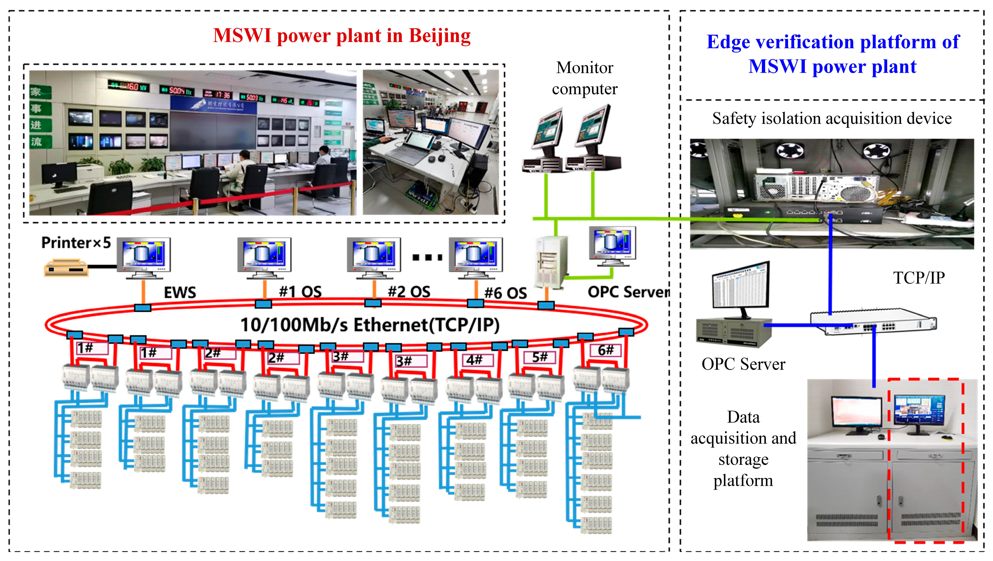
The data in this article were sourced from an MSWI power plant in Beijing. The structure of the edge verification platform for realizing real-time data collection is shown in Figure 2.

Based on the above platform, we collected process data for 6 consecutive hours from 8:00 to 24:00 on a day in March 2021 from an MSWI plant in Beijing. After averaging and removing outliers, we obtained real data and used them as the basis to build our model, which we subsequently developed into software for real-time data transmission on the platform. The green in the picture represents internal network cable communication, and the blue represents external network cable communication

The industrial analysis and elemental analysis of MSW are shown in

Table 1. Elemental analysis of MSW.

Analysis Type	Components and Elements	Value	Unit
Industrial Analysis	Moisture content	36.3	%
	Fixed carbon	14.16	%
	Volatiles	60.08	%
	ASH	25.76	%
Elemental Analysis	C	47.66	%
	H	6.17	%
	N	0.33	%
	Cl	0.88	%
	S	0.17	%
	O	19.91	%

.

The process parameter values that mainly characterize its operating benchmark conditions are as follows: the primary air temperature is 473 K, and its air volume is 65,400 Nm³/h, accounting for 91.00% of the total air volume; the temperature of the secondary air is 312.5 K, and its air volume is 5580 Nm³/h, accounting for 8.50% of the total air volume; the excess air coefficient is 0.85; the airflow ratio of the grate in the drying section, combustion section one, combustion section two, and burnout section is 0.2431:0.435:0.1927:0.1307, with specific values of 15,900 Nm³/h, 28,350 Nm³/h, 12,600 Nm³/h, and 8550 Nm³/h; the incineration amount is set to 72% of the rated amount, which means the feed rate is 24,000 kg/h; the grate speed is 7.5 m/h; the initial layer thickness is 584.48 mm. The furnace specification and benchmark operating parameters are shown in

Table 2. Furnace specification and benchmark operating parameters.

Parameter	Value	Unit
Rated processing capacity	800	t/d
Actual processing capacity	624	t/d
Grate type	Reciprocating grate furnace	—
Grate L×W	11 × 12.9	m
Grate speed	7.5	m/h
Primary airflow	65,400	Nm3/h
Secondary airflow	5580	Nm3/h
Primary air temperature	473	°C
Urea solution	20,000	Kg/h

.

2.4. Modeling Strategy

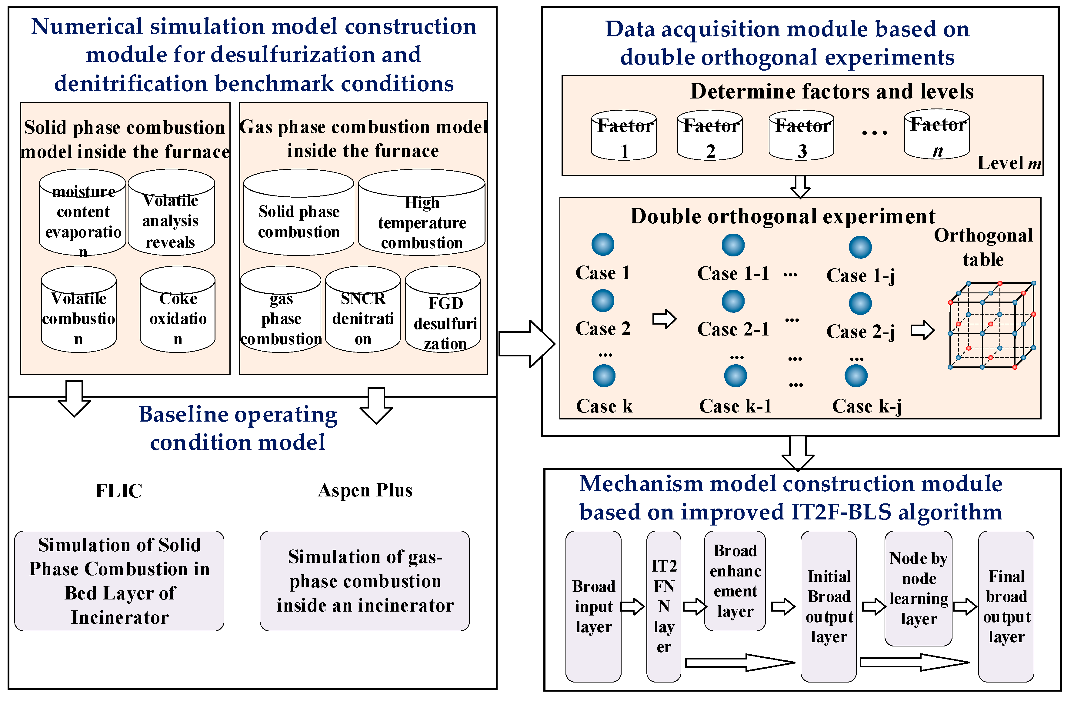
The proposed strategy is shown in Figure 3, including the numerical simulation model construction module for desulfurization and denitrification benchmark conditions, the data acquisition module based on double orthogonal experiments, and the mechanism model construction module based on an improved IT2FBLS algorithm.

In Figure 3, the functions of the different modules are as follows:

(1)

Numerical simulation model construction module for desulfurization and denitrification benchmark conditions: The module includes the development and solution of numerical simulation models for FLIC and Aspen Plus V12.1. FLIC is used to simulate the solid-phase combustion process of MSW in the bed, while Aspen Plus is employed to model the gas-phase combustion process and the pollutant removal reactions within the furnace.

(2)

Data acquisition module based on double orthogonal experiments: Adopting a double orthogonal experimental design for the above 10 factors, the virtual simulation data samples are obtained.

(3)

Mechanism model construction module based on an improved IT2FBLS algorithm: By utilizing the data obtained from orthogonal experiments as the dataset for prediction, a mechanism model related to desulfurization and denitrification pollutant concentrations is constructed based on an improved IT2FBLS algorithm.

2.5. Strategy Implementation

A.

Numerical simulation model construction module for desulfurization and denitrification benchmark conditions

We adopt a multi-software coupling mode to simulate the internal combustion process of the incinerator, which is divided into a solid-phase combustion process on the bed and a gas-phase combustion process above the grate. The solid-phase combustion process on the bed is numerically simulated using FLIC, and the calculation results are imported into Aspen Plus V12.1 as the boundary conditions for the grate bed inlet. Then, a gas-phase combustion simulation is carried out in Aspen Plus V12.1. Considering the uncertainty of MSW composition and the complexity of the combustion process, a steady-state analysis is conducted under the following assumptions: the incinerator is in a stable operating state, the reactions inside the furnace can reach equilibrium, and the temperature and pressure of each reactor are constant without considering pressure loss and heat loss; during the entire incineration process, assuming uniform air distribution, it can fully react with MSW; the main components of MSW are C, H, O, N, S, and Cl, among which C is converted into gas and ash; ash does not participate in the reaction; the gas-phase N element reacts to generate gas compounds; solid N reacts alone to generate NO; the S element generates SO₂ and SO₃; the Cl element generates HCl. Due to the complex composition of tar, its related reactions are not included in the simulation process.

(1)

Solid-state combustion simulation based on FLIC

When MSW enters the incinerator from the feeder, it is first subjected to radiation heating on the bed, and water is released as evaporation proceeds. The release rate can be expressed as follows:

$$\begin{array}{c}{R}_{\mathrm{evp}}=S_{\mathrm{a}}{h}_{\mathrm{s}}(C_{\mathrm{w},\mathrm{s}}-C_{\mathrm{w},\mathrm{g}}), T_{\mathrm{s}}<100 °\mathrm{C}\\ R_{\mathrm{evp}}=Q_{\mathrm{cr}}/H_{\mathrm{evp}},T_{\mathrm{s}}=100 °\mathrm{C}\end{array},$$

(7)

where $R_{\mathrm{evp}}$ represents the rate of the water evaporation reaction; $S_{\mathrm{a}}$ is the surface area of the particles; $H_{\mathrm{evp}}$ represents the heat generated by the evaporation of solid moisture; $T_{\mathrm{s}}$ is the MSW temperature; $h_{\mathrm{s}}$ is the convective mass transfer coefficient between a solid and gas; $C_{\mathrm{w},\mathrm{s}}$ and $C_{\mathrm{w},\mathrm{g}}$ are the water concentrations in the solid and gas phases, respectively; $Q_{\mathrm{cr}}$ is the amount of heat absorbed by convective and radiative heat transfer solids, as follows:

$$Q_{\mathrm{cr}}=S_{\mathrm{a}}(h_{\mathrm{s}}^{\prime }(T_{\mathrm{g}}-T_{\mathrm{s}})+{\epsilon }_{\mathrm{s}}{\sigma }_{\mathrm{b}}(T_{\mathrm{env}}^4-T_{\mathrm{s}}^4)),$$

(8)

where ${\epsilon }_{\mathrm{s}}$ represents the solid emissivity; ${\sigma }_{\mathrm{b}}$ is the Boltzmann radiation constant; $T_{\mathrm{g}}$ is the gas temperature; $T_{\mathrm{env}}$ represents the ambient temperature; $h_{\mathrm{s}}^{\prime }$ is the convective heat transfer coefficient between solid and gas.

After the evaporation of water, dry MSW begins to release volatile compounds at high temperatures, mainly composed of trace compounds such as hydrocarbons (CmHn), CO, CO₂, H₂, O₂, etc., as follows:

$$\mathrm{MSW}\to \mathrm{Volatile}\left({\mathrm{C}}_{\mathrm{m}}{\mathrm{H}}_{\mathrm{n}},\mathrm{CO},{\mathrm{CO}}_2,{\mathrm{H}}_2\mathrm{O}\right)+\mathrm{Char}.$$

(9)

Using a relatively simple and accurate one-step global reaction model [24], the release rate of volatile matter is proportional to the remaining volatile matter and temperature, as shown in the following equation:

$$R_{\mathrm{V}}={\rho }_{\mathrm{sb}}(v_{\infty }-v)A_{\mathrm{V}}\exp \left(-{\displaystyle \frac{E_{\mathrm{V}}}{R{T}_{\mathrm{s}}}}\right),$$

(10)

where $R_{\mathrm{V}}$ represents the reaction rate of volatile matter; $v_{\infty }$ is the final yield of volatile matter; $v$ is the release amount of volatile matter at time; $R$ is the universal gas constant; $A_{\mathrm{V}}$ represents the pre-exponential factor of volatile combustion rate; $E_{\mathrm{V}}$ is the activation energy.

The gas released by high-temperature MSW in the furnace mixes with the surrounding air and rapidly burns. Simplified gaseous combustible volatiles include CmHn and CO, and their combustion reactions are as follows:

$${\mathrm{C}}_{\mathrm{m}}{\mathrm{H}}_{\mathrm{n}}+\left(m/2+n/4\right){\mathrm{O}}_2\to m\mathrm{CO}+n/2{\mathrm{H}}_2\mathrm{O},$$

(11)

$$\mathrm{CO}+1/2{\mathrm{O}}_2\to {\mathrm{CO}}_2.$$

(12)

The combustion rate or kinetic rate related to temperature is provided by the following equations:

$$R_{{\mathrm{C}}_{\mathrm{m}}{\mathrm{H}}_{\mathrm{n}}}=59.8T_g{P}^{0.3}{C}_{{\mathrm{C}}_{\mathrm{m}}{\mathrm{H}}_{\mathrm{n}}}^{0.5}{C}_{{\mathrm{O}}_2}\exp \left(-12200/T_g\right),$$

(13)

$$R_{\mathrm{CO}}=1.3\times {10}^{11}{C}_{\mathrm{CO}}{C}_{{\mathrm{H}}_2\mathrm{O}}^{0.5}{C}_{{\mathrm{O}}_2}^{0.5}.$$

(14)

The combustion of combustible volatile gases is not only limited by reaction kinetics but also by the mixing rate of combustible gases with surrounding air. Assuming that the mixing rate inside the bed is proportional to the energy loss through the bed, the mixing rate can be expressed as follows:

$$R_{\mathrm{mix}}=C_{\mathrm{mix}}{\rho }_{\mathrm{g}}\left\{150{\displaystyle \frac{D_{\mathrm{g}}{(1-\varphi )}^{2/3}}{d_{\mathrm{p}}^2\varphi }}+1.75{\displaystyle \frac{V_g{(1-\varphi )}^{1/3}}{d_{\mathrm{p}}\varphi }}\right\}\min \left\{{\displaystyle \frac{C_{\mathrm{fuel}}}{S_{\mathrm{fuel}}}},{\displaystyle \frac{C_{{\mathrm{O}}_2}}{S_{{\mathrm{O}}_2}}}\right\},$$

(15)

where $C_{\mathrm{mix}}$ is an empirical constant, $C$ is the mass fraction of gaseous reactants, $D_{\mathrm{g}}$ is the gas mass diffusion coefficient, $V_g$ is the air velocity, ${\rho }_{\mathrm{g}}$ is the gas density, $d_{\mathrm{p}}$ is the particle diameter, $\varphi$ is the bed void ratio, and $S$ is the stoichiometric coefficient in the reaction.

The actual combustion reaction rate of volatile matter is taken as the minimum value of the temperature-related kinetic rate $R_{\mathrm{kinetics}}$ and oxygen mixing rate $R_{\mathrm{mix}}$, as shown in the following equation:

$$R=\min \left(R_{\mathrm{kinetics}},R_{\mathrm{mix}}\right).$$

(16)

During volatilization analysis, MSW particles will form coke, and the main products of further gasification are CO and CO₂. The reaction equation can be expressed as follows:

$$\mathrm{C}\left(\mathrm{s}\right)+\alpha {\mathrm{O}}_2\to 2\left(1-\alpha \right)\mathrm{CO}+\left(2\alpha -1\right){\mathrm{CO}}_2,$$

(17)

where the range of coefficient $\alpha$ is 0.5–1, which can be determined according to Arthur’s law.

The rate of coke combustion can be expressed as follows:

$$R_{\mathrm{C}}={\displaystyle \frac{P_{{\mathrm{O}}_2}}{\frac{1}{k_{\mathrm{r}}}+\frac{1}{k_{\mathrm{d}}}}},$$

(18)

where $R_{\mathrm{C}}$ is the reaction rate of coke combustion; $P_{{\mathrm{O}}_2}$ is the partial pressure of oxygen; $k_{\mathrm{r}}$ and $k_{\mathrm{d}}$ are the rate constants caused by chemical kinetics and diffusion, respectively.

At the initial stage of model construction, a one-step reaction model with a simplified form (e.g., volatile release rate is exponentially related to remaining volatiles and temperature) is preferred to quickly validate the feasibility of the coupling framework between FLIC and Aspen Plus. This simplified treatment aims to reduce the initial complexity of the multi-software coupling and focuses on the construction of the full life cycle modeling framework. Subsequently, we will refer to the subdivision method of pyrolysis behavior of solid waste components and the idea of kinetic parameter calibration in the study of Dong et al. [25] to improve the accuracy of solid-phase combustion simulation.

(2)

Gas phase combustion simulation based on Aspen Plus

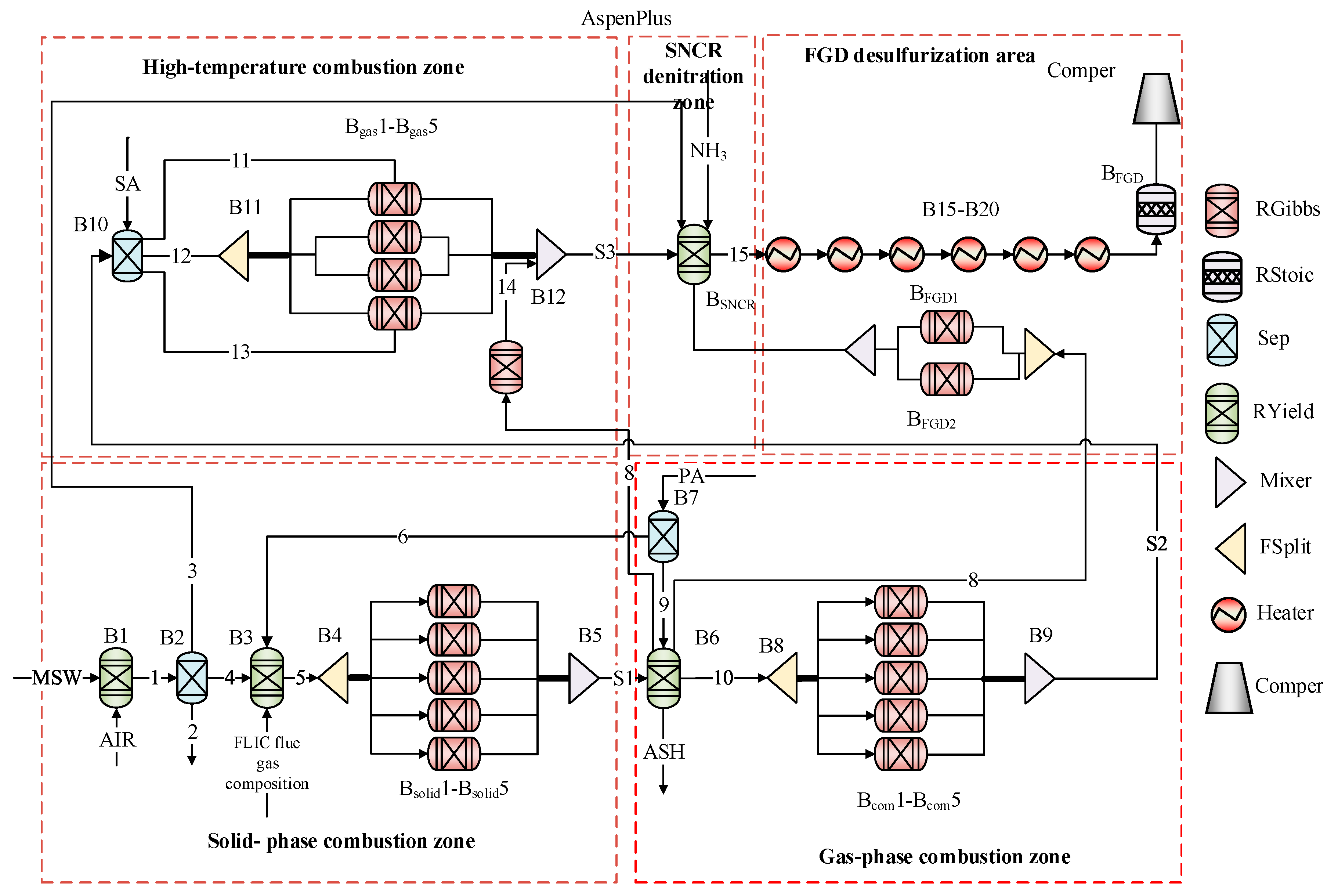
The overall numerical simulation model of gas-phase combustion based on Aspen Plus is shown in Figure 4.

In Figure 4, the numerical simulation model comprises a solid-phase combustion zone, a gas-phase combustion zone, a high-temperature combustion zone, an SNCR desulfurization zone, and an FGD desulfurization zone. Its coupling with FLIC is demonstrated by obtaining the solid-phase combustion flue gas components from FLIC and inputting them into the B3 module. The output of the B3 module is then mixed with primary air and fed into subsequent modules for further experimentation. The functions of each module are outlined in

Table 3. Functions of each module in the numerical simulation model based on Aspen Plus.

Module	Name	Role
B1	Yield Reactor	Simulate the drying process of MSW
B2	Splitter	Drain dry water and debris
B3	Yield Reactor	Simulation of gas-phase reaction after primary wind input
B4, B8, B11	Splitter	Splitting of gases
B5, B9, B12	Mixer	Mixing of gas streams
Bsolid1–Bsolid5	Gibbs reactor	Simulation of solid-phase combustion gas reactions
B6	Splitter	Separation of slag from solid-phase combustion
B7	Splitter	Diversion of primary airflow
Bcom1–Bcom5	Gibbs reactor	Simulation of gas-phase combustion reactions
B10	Splitter	Separation of NH3 and HCN
Bgas1–Bgas5	Gibbs reactor	Simulation of high-temperature combustion zone reactions
BSNCR	Yield Reactor	Simulation of SNCR purification reaction
BFGD1.2	Yield Reactor	Simulation of FGD desulfurization reaction
B15–B20	Heat exchangers	Simulation of superheater and economizer cooling

.

(1)

Solid phase combustion zone: In the numerical simulation of this zone, MSW first enters the drying module B1, where moisture is removed through B2. The dried MSW then enters B3, where it is mixed with primary air. After passing through splitter B4, the mixture flows into reactors Bsolid1-Bsolid5 for solid-phase combustion simulation. These reactors simulate the generation of conventional gas products such as NO₂, NO, HCN, NH₃, SO₂, SO₃, HCl, and others. The generation ratio of HCN and NH₃ is set to 9. Finally, the products from all modules flow into mixer B5, where the relevant reactions occur:

$$MSW\to {NO}_2+NO+N_{2}O+HCN+N{H}_3+\dots$$

(19)

(2)

Gas-phase combustion zone: This zone simulates the reactions that occur as MSW enters the grate and heats up to 500 °C. First, the products from the solid-phase combustion zone flow into separator B6, where solid slag such as ASH is discharged. Next, char-N is directed into reactor Bgas5, while the remaining gas is mixed with primary air and flows into diverter B8. After diversion, the gas enters reactors Bcom1-Bcom5 to simulate gas-phase combustion reactions. Finally, the products from all modules are mixed after entering mixer B9. The relevant reactions are as follows:

$$3H_2+N_2=2{NH}_3,$$

(20)

$${NH}_3+CO=HCN+H_{2}O,$$

(21)

$$NO+{CH}_4=H_{2}O+H2+HCN,$$

(22)

$$CO/H_2+NO\to HCN/N_{2}O.$$

(23)

(3)

High-temperature combustion zone: This zone simulates the process when the furnace temperature ranges between 500 °C and 800 °C. Initially, the gas-phase combustion products and secondary air flow into separator B10, where they are mixed and separated, with HCN and NH₃ being isolated from other conventional gases. The separated NH₃ and HCN then flow into reactors Bgas1 and Bgas4. The remaining gases are split by splitter B11 and directed into reactors Bgas1-Bgas4 for high-temperature combustion simulation. The main reactions are as follows:

$$HCN+O_2\to NO+\dots ,$$

(24)

$$HCN+NO\to N_2+\dots ,$$

(25)

$$N{H}_3+O_2\to NO+\dots ,$$

(26)

$$N{H}_3+NO\to N_2+\dots .$$

(27)

In addition to NO₂ being reduced to NO at temperatures above 600 °C, this zone also contains some reducing gases that reduce NOx, such as CO’s reduction reaction with NO [26]:

$$2CO+2NO\to N_2+2C{O}_2.$$

(28)

In addition, Char-N, which is separated from the gas-phase combustion zone and flows into Bgas5, undergoes the following decomposition reaction:

$$C\mathrm{har}-N\to NO.$$

(29)

Finally, all products flow into mixer B12 together.

This module is the location with the highest NOx concentration in the whole MSWI process because, at this temperature, many intermediate products like HCN and NH₃ are decomposed into NOx. Additionally, fixed nitrogen undergoes conversion reactions. In this zone, sulfur (S) appears in the form of SO₂ and SO₃, while chlorine (Cl) is present as HCl and Cl₂.

(4)

SNCR denitration zone: This zone simulates the SNCR denitrification process. First, the products from the high-temperature combustion zone enter the B_SNCR yield reactor, where water and NH₃ are also introduced. The main reactions are as follows:

$$4NO+4N{H}_3+O_2=4N_2+6H_{2}O,$$

(30)

$$2NO+4N{H}_3+2O_2=3N_2+6H_{2}O,$$

(31)

$$6N{O}_2+8N{H}_3=7N_2+12H_{2}O.$$

(32)

Furthermore, the gas processed by the SNCR enters reactors B15-B20 to simulate the cooling effect of the three-stage superheater and three-stage economizer, before finally flowing into the subsequent modules.

(5)

FGD desulfurization zone: This zone simulates the FGD desulfurization process. The purified gas from the SNCR process flows into B_FGD1 and B_FGD2, where lime is injected for the desulfurization reaction. The main reactions are as follows:

$$S{O}_2+Ca{(OH)}_2=CaS{O}_3+H_{2}O,$$

(33)

$$S{O}_3+Ca{(OH)}_2=CaS{O}_4+H_{2}O,$$

(34)

$$2HCl+Ca{(OH)}_2=CaC{l}_2+2H_{2}O,$$

(35)

The generation and consumption of HCN, NH₃ and other intermediates in the waste incineration process have significant time-dependence (e.g., the HCN release rate in the solid-phase combustion stage varies with the time of grate advancement, and the reaction rate of NH₃ with NO_x in the SNCR region fluctuates with the residence time), and the existing models do not adequately quantify this dynamic property, which may lead to the prediction bias of pollutant concentrations. The “generalized solution method of spatio-temporally dependent source terms” proposed by Ding et al. [27] provides an important idea to deal with such problems, which is especially suitable for the mathematical description of unsteady reaction processes, and we will focus on solving these problems in the future.

B.

Data acquisition module based on double orthogonal experiments

This article adopts a double orthogonal experimental design to obtain multiple sets of manipulated and non-manipulated variable values under various operating conditions. The process is as follows:

(1)

We determine the experimental factor $n$ and its level $m$, and then we obtain the orthogonal experimental table ${\mathrm{L}}_K(m^n)$. This provides $K$ experimental cases that can be obtained.

(2)

Based on the $K$ cases obtained from the first orthogonal experiment, the experimental factor $n_1$ and its level $m_1$ are re-determined to obtain $K$ orthogonal experimental tables ${\mathrm{L}}_L({m_1}^{n_1})$.

(3)

The $K\times L$ experimental case can be obtained, with a total of $K\times L$ operating conditions.

The $K\times L$ experimental cases obtained above are sequentially input into the multi-software coupled desulfurization and denitrification numerical simulation model $f_{\mathrm{model}}\left(\cdot \right)$, which can be expressed as follows:

$$y_{\mathrm{model}}=f_{\mathrm{model}}\left(x_{\mathrm{feed}},x_{\mathrm{speed}},x_{\mathrm{air}1},x_{\mathrm{moisture}},x_{\mathrm{particle}},x_{\mathrm{mix}},x_{\mathrm{air}2},x_{\mathrm{sat}},x_{\mathrm{NH}3},x_{\mathrm{Ca}\left(\mathrm{OH}\right)2}\right),$$

(36)

where $x_{\mathrm{feed}}$, $x_{\mathrm{speed}}$, $x_{\mathrm{air}1}$, $x_{\mathrm{moisture}}$, $x_{\mathrm{particle}}$, $x_{\mathrm{mix}}$, $x_{\mathrm{air}2}$, $x_{\mathrm{sat}}$, $x_{{\mathrm{NH}}_3}$, and $x_{{\mathrm{Ca}\left(\mathrm{OH}\right)}_2}$ represent the feed rate amount, grate speed, primary air volume in the drying section, moisture content, particle size, particle mixing coefficient, secondary air volume, secondary air temperature, urea feeding flow rate, and lime feeding amount, respectively; $f_{\mathrm{model}}\left(\cdot \right)$ represents the coupled numerical simulation model constructed in the previous text; $y_{\mathrm{model}}$ represents the concentration of relevant pollutants for coupling numerical simulation models.

At this point, virtual simulation mechanism data of desulfurization and denitrification-related pollutants under the conditions $K\times L$ have been obtained.

C.

Mechanism model construction module based on an improved IT2FBLS algorithm

The improved IT2FBLS network consists of two main phases: the training phase and the hierarchical incremental learning phase. The model training phase includes a width input layer, an IT2FNN layer, a width enhancement layer, and an initial width output layer. The hierarchical incremental learning phase consists of a node-by-node learning layer and a final width output layer.

(1)

Model training phase

In the broad input layer, it does not transform the input data, which can be represented as follows:

$$\left\{\begin{array}{c}{\left\{{\mathit{x}}_n^{\mathrm{mix}}\right\}}_{n=1}^N={\left[x_1,x_2,\dots ,x_N\right]}^{\mathrm{T}}\in {ℝ}^{N\times M}\\ x_s=\left[x_s^1,x_s^2,\dots ,x_s^M\right],s=1,2,\dots ,N\end{array}\right.,$$

(37)

where $N$ represents the number of samples, and $M$ represents the number of features of the input data.

The IT2FNN layer contains $I$ subsystems. By taking the $n$-th sample of the $i$-th subsystem as an example, the details are shown as follows. In the antecedent network, the input layer passes the network input to the membership function layer, with a weight of 1 and a node count of $M$. The membership function layer fuzzifies the input variables and represents them in interval form, with a weight of 1 and several nodes $M\times K$ (representing the number of fuzzy rules), where each node represents an interval type-2 membership function. The input of this layer is the output of the input layer, which is the membership degree of the fuzzy set. After using Gaussian membership functions with uncertain mean to calculate the membership degree of a fuzzy set [28], by taking the membership degree of the rule $k$ corresponding to the $m$-th input as an example, the lower and upper bounds are calculated as follows:

$${\underset{\_}{\mu }}_{n_{m}k}^i=\left\{\begin{array}{l}\exp \left[-{\displaystyle \frac{1}{2}}{\left({\displaystyle \frac{x_{n_m}^i-{\overline{c}}_{n_{m}k}^i}{{\sigma }_{n_{m}k}^i}}\right)}^2\right], x_{n_m}^i\le {\displaystyle \frac{{\underset{\_}{c}}_{n_{m}k}^i+{\overline{c}}_{n_{m}k}^i}{2}}\\ \exp \left[-{\displaystyle \frac{1}{2}}{\left({\displaystyle \frac{x_{n_m}^i-{\underset{\_}{c}}_{n_{m}k}^i}{{\sigma }_{n_{m}k}^i}}\right)}^2\right], x_{n_m}^i>{\displaystyle \frac{{\underset{\_}{c}}_{n_{m}k}^i+{\overline{c}}_{n_{m}k}^i}{2}}\end{array}\right.,$$

(38)

$${\overline{\mu }}_{n_{m}k}^i=\left\{\begin{array}{l}\exp \left[-{\displaystyle \frac{1}{2}}{\left({\displaystyle \frac{x_{n_m}^i-{\underset{\_}{c}}_{n_{m}k}^i}{{\sigma }_{n_{m}k}^i}}\right)}^2\right],x_{n_m}^i<{\underset{\_}{c}}_{n_{m}k}^i\\ \hspace{1em}\hspace{1em}\hspace{0.17em}\hspace{0.17em}\hspace{0.17em}\hspace{0.17em}\hspace{0.17em}\hspace{0.17em}\hspace{0.17em}\hspace{0.17em}1\hspace{0.17em}\hspace{0.17em}\hspace{0.17em}\hspace{0.17em}\hspace{0.17em},{\underset{\_}{c}}_{n_{m}k}^i\le x_{n_m}^i<{\overline{c}}_{n_{m}k}^i\\ \exp \left[-{\displaystyle \frac{1}{2}}{\left({\displaystyle \frac{x_{n_m}^i-{\overline{c}}_{n_{m}k}^i}{{\sigma }_{n_{m}k}^i}}\right)}^2\right],x_{n_m}^i\ge {\overline{c}}_{n_{m}k}^i\end{array}\right.,$$

(39)

where $x_{n_m}^i$ represents $m$ input variables; ${\underset{\_}{c}}_{n_{m}k}^i$ and ${\overline{c}}_{n_{m}k}^i$, respectively, represent the lower and upper bounds of the uncertainty center of the $k$-th membership function corresponding to the $m$-th input variable; ${\sigma }_{n_{m}k}^i$ represents the width of the $k$-th membership function corresponding to the $m$-th input variable.

The fuzzy rule layer constructs fuzzy rules and implements fuzzy inference calculation, with a weight of 1 and a node number of $K$. The input of this layer is the output of the membership function layer, and the output is the activation strength of the fuzzy rules. Taking the $k$-th fuzzy rule as an example, the calculation is as follows:

$$F_k^i=\left[{\underset{\_}{f}}_k^i,{\overline{f}}_k^i\right],$$

(40)

$${\underset{\_}{f}}_k^i={\displaystyle \prod _{m=1}^M{\underset{\_}{\mu }}_{n_{m}k}^i={\underset{\_}{\mu }}_{n_{1}k}^i\times {\underset{\_}{\mu }}_{n_{2}k}^i\times \cdot \cdot \cdot \times {\underset{\_}{\mu }}_{n_{M}k}^i},$$

(41)

$${\overline{f}}_k^i={\displaystyle \prod _{m=1}^M{\overline{\mu }}_{n_{m}k}^i={\overline{\mu }}_{n_{1}k}^i\times {\overline{\mu }}_{n_{2}k}^i\times \cdot \cdot \cdot \times {\overline{\mu }}_{n_{M}k}^i},$$

(42)

where ${\underset{\_}{f}}_k^i$ and ${\overline{f}}_k^i$ represent the lower and upper bounds of the activation strength of rule $k$, respectively.

The activation strength and consequent parameters of the descent layer combination rule complete the descent operation, and the weight is the weight of the consequent interval with 2 nodes. The input of this layer is the output of the fuzzy rule layer, which outputs the lower and upper bounds of the subsystem feature mapping. The calculation is as follows:

$${\underset{\_}{z}}_{n_m}^i={\displaystyle \frac{{\displaystyle \sum _{k=1}^K{\underset{\_}{f}}_k^i{\delta }_k^i}}{{\displaystyle \sum _{k=1}^K{\underset{\_}{f}}_k^i}}},$$

(43)

$${\overline{z}}_{n_m}^i={\displaystyle \frac{{\displaystyle \sum _{k=1}^K{\overline{f}}_k^i{\delta }_k^i}}{{\displaystyle \sum _{k=1}^K{\overline{f}}_k^i}}},$$

(44)

where ${\delta }_k^i$ represents the weight of the consequent interval.

The output layer is de-fuzzified to obtain the model output, with weights of the lower-bound proportional value $q$ and the upper-bound proportional value $\left(1-q\right)$. The input of this layer is the output of the descent layer, and the output is the feature mapping result. The calculation is as follows:

$$z_{n_m}^i=q{\underset{\_}{z}}_{n_m}^i+(1-q){\overline{z}}_{n_m}^i.$$

(45)

In the consequent network, the input layer passes the network output to the subsequent network. The hidden layer contains $K$ node and outputs the weights of fuzzy rules in the antecedent network, which can be expressed as follows:

$${\delta }_k^i=b_k^i+{\displaystyle \sum _{m=1}^M{v}_{n_m}^i{\omega }_{n_{m}k}^i},$$

(46)

where ${\delta }_k^i$ represents the output of the $k$-th node, which is the output weight of the $k$-th rule in the antecedent network; $b_k^i$ represents the bias of the $k$-th node; ${\omega }_{n_{m}k}^i$ represents the weight from the $m$-th input to the $k$-th node; $v_{n_m}^i$ represents the $m$-th input. Furthermore, the feature mapping output of the subsystem can be represented as follows:

$$Z_i={\left[z_1^i,\dots ,z_n^i,\dots ,z_N^i\right]}^{\mathrm{T}},$$

(47)

where $z_n^i={\left[z_{n_1}^i,\dots ,z_{n_m}^i,\dots ,z_{n_M}^i\right]}^{\mathrm{T}}$. Finally, the output of the IT2FNN layer can be represented as follows:

$${\left\{{\mathit{Z}}_i\right\}}_{i=1}^I=\left[Z_1,\dots ,Z_i,\dots ,Z_I\right].$$

(48)

The broad enhancement layer contains $L$ number of enhanced nodes, and the output of the IT2FNN layer is nonlinearly transformed using the $\tan \mathrm{sig}$ function, which can be expressed as follows:

$${\left\{{\mathit{H}}_l\right\}}_{l=1}^L=\left[H_1,H_2,\dots ,H_L\right],$$

(49)

$$H_l={\xi }_l\left(Z{W}_{hl}+{\beta }_{hl}\right),\hspace{0.17em}\hspace{0.17em}l=1,2,\dots ,L,$$

(50)

where $W_{hl}$ and ${\beta }_{hl}$ represent the randomly generated connection weights and biases of the i-th enhancement node in the IT2FNN layer and enhancement layer, respectively.

The initial broad output layer contains 3 nodes, and its output can be represented as follows:

$$\widehat{Y}=Z{W}_f+H{W}_e=[Z,H]\left[\begin{array}{l}{W}_f\\ W_e\end{array}\right]=AW,$$

(51)

where $W_f$ and $W_e$ represent the connection weights between the IT2FNN layer and the enhancement layer and the output layer, respectively; $\widehat{Y}$ represents the network output during the training phase; $\mathit{A}$ represents the network input; $W$ represents the network connection weights. According to Equation (51), we can obtain the following:

$$\mathit{W}={\mathit{A}}^{+}\mathit{Y},$$

(52)

where ${\mathit{A}}^{+}$ represents the generalized inverse matrix, and $\mathit{Y}$ represents the true value of the model.

Due to the difficulty in directly obtaining ${\mathit{A}}^{+}$ practical problems, $L^2$ regularization is used to transform them into an optimization problem, whose expression is the following:

$$\underset{\mathit{W}}{\arg \min }{‖\mathit{A}\mathit{W}-\mathit{Y}‖}_2^2+\lambda {‖\mathit{W}‖}_2^2,$$

(53)

where $\lambda$ represents the regularization coefficient, and $\lambda >0$. Furthermore, by using ridge regression estimation, the Moore–Penrose inverse matrix ${\mathit{A}}^{+}$ is obtained as follows:

$${\mathit{A}}^{+}=\underset{\lambda \to 0}{\lim }{\left(\lambda \mathit{I}+\mathit{A}{\mathit{A}}^T\right)}^{-1}{\mathit{A}}^T,$$

(54)

where $I$ represents the identity matrix. Finally, the calculation $W$ is as follows:

$$\mathit{W}={\left(\lambda I+A{A}^{\mathrm{T}}\right)}^{-1}{A}^{\mathrm{T}}Y.$$

(55)

(2)

Hierarchical incremental learning phase

For the node-by-node learning layer, based on the feature nodes and enhancement nodes in the training phase, the $Q$ layer is divided for hierarchical incremental learning ($Q$ represents the number of network outputs). By taking the $q$-th output as an example, the node-by-node learning process is described as follows.

First, we calculate the mean square error (MSE) between the $q$-th output and the true value, expressed as follows:

$$MS{E}_q^p={\displaystyle \frac{1}{N}}{\displaystyle \sum _{n=1}^N{\left({\widehat{y}}_n-y_n\right)}^2},$$

(56)

where $MS{E}_q^p$ represents the mean square error of the $q$-th output after adding $p$ enhancement nodes; ${\widehat{y}}_n$ and $y_n$ represent the output and truth of the $n$-th sample model, respectively.

Then, we calculate the MSE increment before and after adding the enhancement node to the $q$-th output, which is expressed as follows:

$${\delta }_q=\left|MS{E}_q^p-MS{E}_q^{p+1}\right|.$$

(57)

If ${\delta }_q$ does not meet the set threshold $\theta$, the incremental learning process is performed on the $q$-th output enhancement node of the network. The augmentation matrix is updated as follows:

$${\mathit{A}}_{\mathrm{new}}^q=\left[\mathit{A}\left|{\xi }_{\left(L+1\right)}^q\left(\mathit{Z}{\mathit{W}}_{h\left(L+1\right)}^q+{\mathit{\beta }}_{h\left(L+1\right)}^q\right)\right.\right].$$

(58)

According to Equation (52), the network weight after adding enhanced nodes can be expressed as follows:

$${\mathit{W}}_{\mathrm{new}}^q={\left({\mathit{A}}_{\mathrm{new}}^q\right)}^{+}\mathit{Y}.$$

(59)

The pseudo-inverse matrix of the input matrix after adding enhanced nodes can be expressed as follows:

$${\left({\mathit{A}}_{\mathrm{new}}^q\right)}^{+}=\left[\begin{array}{c}{\mathit{A}}^{+}-D{B}^{\mathrm{T}}\\ B^{\mathrm{T}}\end{array}\right],$$

(60)

where $\mathit{D}={\mathit{A}}^{+}{\xi }_{\left(L+1\right)}\left(\mathit{Z}{\mathit{W}}_{h\left(L+1\right)}+{\mathit{\beta }}_{h\left(L+1\right)}\right)$;

$$B^{\mathrm{T}}=\left\{\begin{array}{l}{\left(C\right)}^{+}\hspace{0.17em}\hspace{0.17em}\hspace{0.17em}\hspace{0.17em}\hspace{0.17em}\hspace{0.17em}\hspace{0.17em}\hspace{0.17em}\hspace{0.17em}\hspace{0.17em}\hspace{0.17em}\hspace{0.17em}\hspace{0.17em}\hspace{0.17em}\hspace{0.17em}\hspace{0.17em}\hspace{0.17em}\hspace{0.17em}\hspace{0.17em}\hspace{0.17em}\hspace{0.17em}\hspace{0.17em}\hspace{0.17em}\hspace{0.17em}if\hspace{0.17em}\hspace{0.17em}\hspace{0.17em}C\ne 0\\ {\left(1+D^{\mathrm{T}}D\right)}^{-1}{D}^{\mathrm{T}}{\left({\mathit{A}}^L\right)}^{+}\hspace{0.17em}\hspace{0.17em}\hspace{0.17em}if\hspace{0.17em}\hspace{0.17em}\hspace{0.17em}C=0\end{array}\right.,$$

(61)

where $C=\xi \left(\mathit{Z}{\mathit{W}}_{h\left(L+1\right)}+{\mathit{\beta }}_{h\left(L+1\right)}\right)-\mathit{A}\mathit{D}$.

Therefore, the weight matrix of the enhanced node after adding the $q$-th output can be expressed as follows:

$${\mathit{W}}_{\mathrm{new}}^q=\left[\begin{array}{c}\mathit{W}-D{B}^{\mathrm{T}}Y\\ B^{\mathrm{T}}Y\end{array}\right].$$

(62)

For the final broad output layer, by repeating the above process until all outputs of ${\delta }_q$ satisfy $\theta$, the weights of the network are obtained. The expression is as follows:

$$\Theta =\psi \left(\mathit{W},{\mathit{W}}_{\mathrm{new}}^1,\dots ,{\mathit{W}}_{\mathrm{new}}^q\right),\hspace{0.17em}q=1,2,\dots ,Q,$$

(63)

where $\psi (\cdot )$ represents the hierarchical incremental learning process.

Finally, the output of the improved IT2FBLS network can be represented as follows:

$${\widehat{\mathit{Y}}}_{\mathrm{new}}=\Theta \mathit{X}.$$

(64)

The existing feature nodes and enhancement nodes during the training process are shared in each layer of hierarchical incremental learning, and the subsequent layer of incremental learning is based on the total number of nodes trained in the previous layer. Therefore, the number of enhancement nodes for the improved IT2FBLS network after training is denoted as $\left(L+p_1+p_2+\cdot \cdot \cdot +p_q\right)$.

2.6. Flow Chart

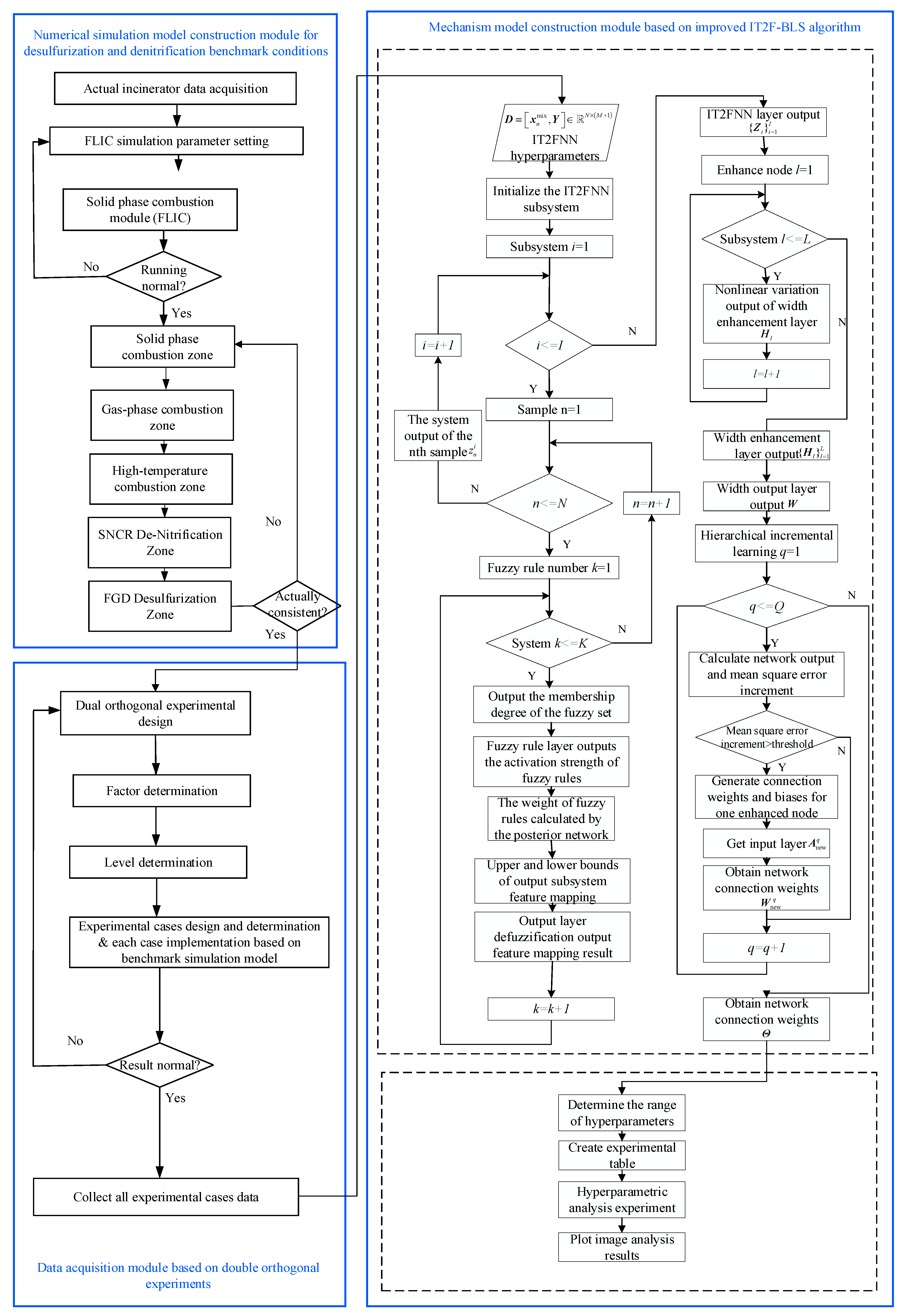
A detailed flowchart of the proposed modeling strategy is shown in Figure 5.

In Figure 5, the flowchart is divided into two parts. The left side mainly consists of a numerical simulation model construction module for desulfurization and denitrification benchmark conditions, and a data acquisition module based on double orthogonal experiments. The right side is the mechanism model construction module based on the improved IT2FBLS algorithm. The main process is as follows:

(1)

Numerical simulation model construction module for desulfurization and denitrification benchmark conditions: First, we use FLIC software to simulate MSW solid-phase combustion and adjust the operating variables until the solid-phase combustion results match the on-site data. Next, the solid-phase simulation results of FLIC are used as boundary conditions for the gas-phase simulation in Aspen Plus. Finally, we adjust the parameters in the gas phase simulation until the results conform to the field data.

(2)

Data acquisition module based on double orthogonal experiments: First, the orthogonal experiment method is used to determine the influencing factors and design a dual orthogonal experiment at different levels. Then, the experiment is conducted to obtain a virtual dataset. Finally, we evaluate the results to determine if they meet the on-site operating conditions.

(3)

Mechanism model construction module based on an improved IT2FBLS algorithm: First, the virtual dataset is divided into a training set, testing set, and validation set. Then, the hyperparameter analysis for an improved IT2FBLS model is presented.

3. Results and Discussion

3.1. Simulation Settings

This article simulates the combustion process of solid-phase MSW in a bed through FLIC simulation. The operating parameters of FLIC under benchmark conditions are shown in

Table 4. Simulation parameter settings for FLIC.

Parameters	Value	Unit
Feed speed	24,000	kg/h
Primary air	65,400	Nm3/h
Primary air temperature	473	°C
Grate speed	7.5	m/h
MSW particle size	25	mm
Mixing factor	2 × 10−6	—
Radiation rate	0.8	—
Moisture content	49.7	—

.

Under the benchmark operating conditions, the gas-phase components simulated by FLIC for solid-phase combustion were selected as boundary conditions to provide MSW for ASPEN simulation. The specific setting parameters of the solid-phase combustion zone module B3 in Aspen are shown in

Table 5. Gas components input into the Aspen Plus numerical simulation model.

Gas Composition	Value	Gas Composition	Value
CH4, mol%	0.02625	CO, mol%	0.03959
CO2, mol%	0.08011	O2, mol%	0.05652
N2, mol%	0.43743	H2O, mol%	0.2814
H2, mol%	0.01424	NO2, mol%	0.01696
HCN, mol%	0.01755	NH3, mol%	0.02994

.

3.2. Experimental Results

A.

Numerical simulation results

(1)

FLIC solid-phase combustion results

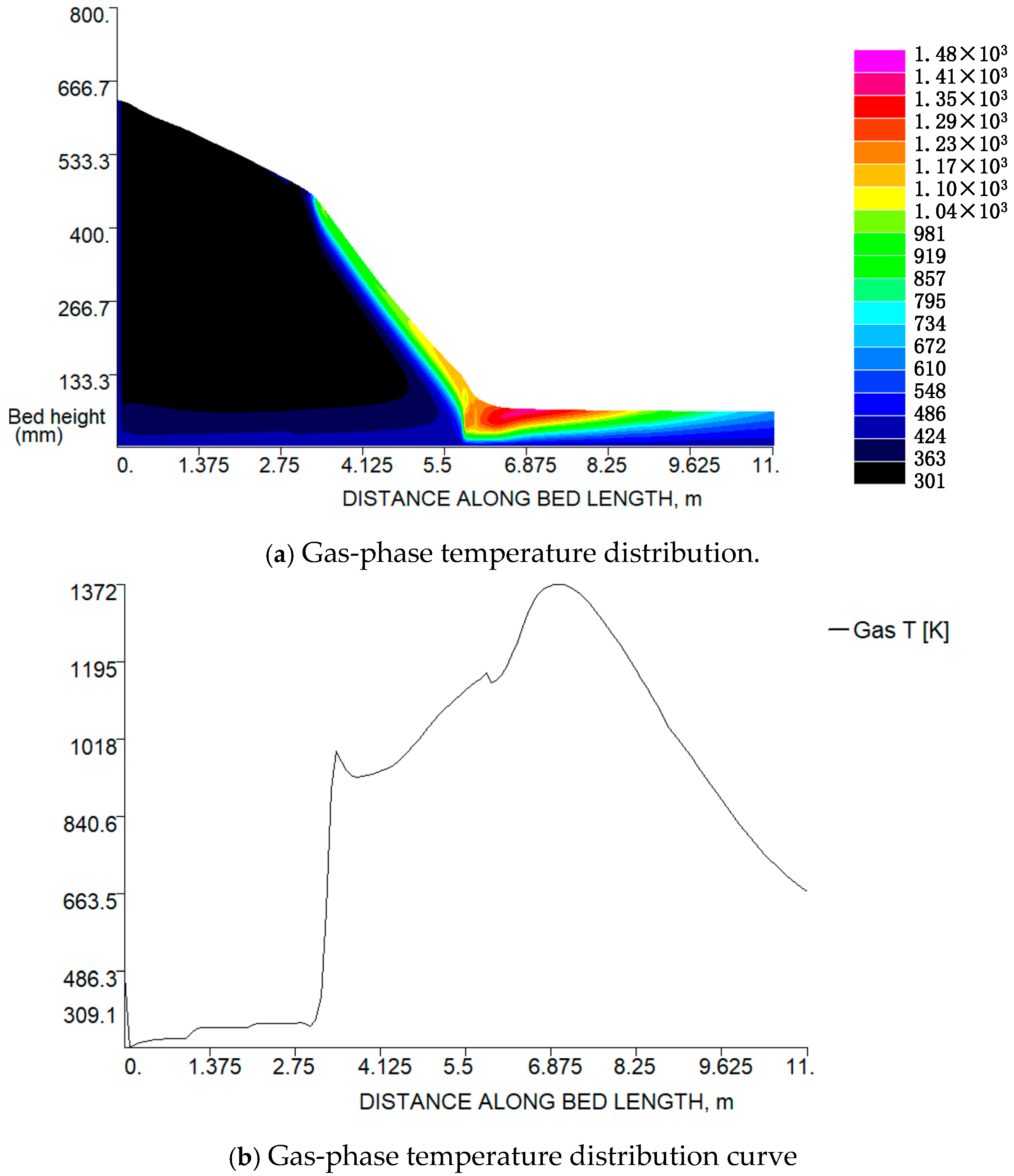
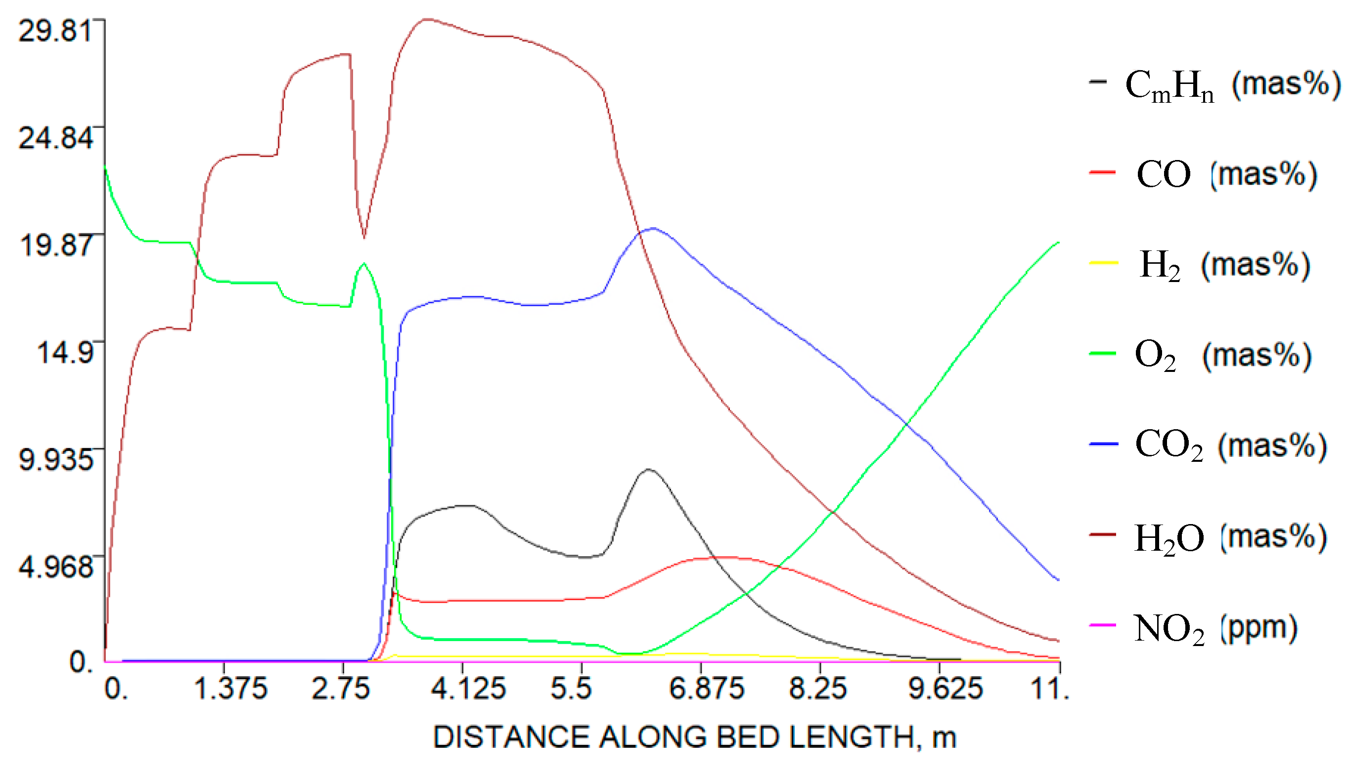
The process rate and gas composition distribution of solid-phase MSW combustion on the grate are shown in Figure 6 and Figure 7.

Figure 6a shows the process rate of solid-phase MSW combustion on the grate and the distribution of gas-phase components. Among them, Figure 6a indicates that the gas-phase high-temperature area above the grate is mainly concentrated behind the drying section, the entire combustion sections 1 and 2, and in front of the burnout section. The core high-temperature area is located in combustion sections 1 and 2. At a grate length of 5.5 m, the gas-phase temperature presents a concentrated and gradually transitional feature. The gas-phase temperature curve in Figure 6b indicates that the temperature gradually increases from 2.8 m of the grate length, reaches the highest point at 6.6 m, and then gradually decreases as the grate length extends. Specifically, the temperature in the front and middle sections of the drying zone is relatively low, generally maintained at 340 K, while the temperature rises rapidly in the rear section of the drying zone and the front section of combustion section 1. After the MSW is dehydrated, it is rapidly ignited at high temperatures, causing the gas-phase temperature in the middle and later sections of combustion section 1 to rise again and reach the maximum value at 6.6 m. The gas-phase temperature in combustion section 2 and the burnout section gradually decreases from a high temperature to about 550 K. The overall temperature change is consistent with the heat release law of the drying, combustion, and burnout processes of the garbage on the grate.

As shown in Figure 7, after MSW enters the incinerator, water evaporates under the action of radiation heat transfer and primary air convection heat transfer. The evaporation rate reaches its peak near 2.75 m of the grate and then gradually decreases to 0. Correspondingly, the mass fraction of H₂O in the flue gas continuously increases before 2.0 m and reaches its peak near 2.75 m. During the drying process, the temperature of the garbage rises. Volatile matter begins to precipitate at 1.3 m of the grate, and the evaporation rate reaches its peak near 6.0 m. Along with the increase in the mass fractions of CO, CmHn, and H₂, the volatile matter and coke combustion generate CO₂, resulting in an increase in the mass fraction of CO₂ and a decrease in the mass fraction of O₂. Coke begins to burn near 3.0 m of the grate and ends at about 9.625 m. During the entire process, the concentration changes in each component are closely related to the stage characteristics of garbage dehydration, pyrolysis, and combustion, which conform to the material transformation law of the municipal solid waste incineration process.

(2)

Aspen Plus gas-phase combustion results

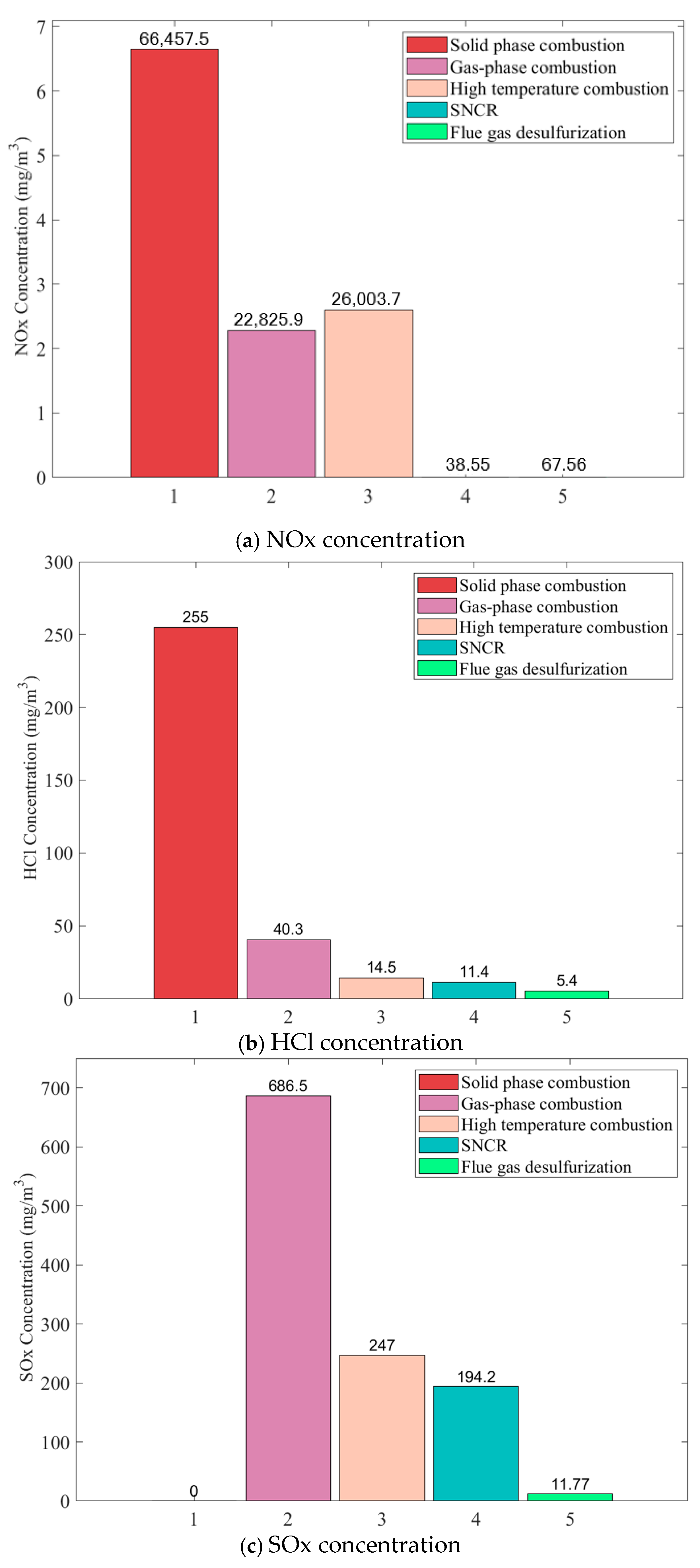
The concentrations of NOx, HCl, and SOx at the outlet of the solid-phase combustion zone, gas-phase combustion zone, high-temperature combustion zone, SNCR denitrification zone, and FGD desulfurization zone under the benchmark operating conditions are shown in Figure 8.

Figure 8 shows that the pollutants are mainly generated in the solid-phase combustion and gas-phase combustion zones. After desulfurization and denitrification treatment, the concentration of the gas shows a significant decreasing trend. A comparison of this result with real plant monitoring data is shown in

Table 6. Comparison of simulated benchmark operating condition results with actual MSWI power plant monitoring records.

	NOx (mg/m3)	Sox (mg/m3)	HCl (mg/m3)
Simulated benchmark operating conditions	67.56	11.77	5.4
Actual MSWI power plant monitoring records	86.75	5.73	4.22

.

B.

Data acquisition results

The orthogonal experiment adopts a double orthogonal design to obtain multiple sets of manipulated and non-manipulated variable values under various operating conditions. The process is as follows:

(1)

Select six experimental factors and the level numbers of five for the first time, design an orthogonal experimental table, and further obtain 49 experimental cases.

(2)

Based on the 49 cases obtained from the first orthogonal experiment, determine the remaining five experimental factors and their level numbers, and obtain an orthogonal experiment table with a quantity of 32.

(3)

Finally, an experimental case can be obtained, with a virtual data volume of 1568 sets obtained through double orthogonal experiments, as shown in

Table 7. Partial case examples of an orthogonal experiment table.

Case #	Grate Speed	Feed Speed	Primary Air	Moisture Content	…	NOx Concentration	HCl Concentration	SOx Concentration
	m/h	t/h	Nkm3/h	%	…	mg/m3	mg/m3	mg/m3
1–1	6.6	24.2	15.3	48	…	279.11	6.49	25
1–2	6.6	24.2	15.3	48	…	845.4	6.5	28.22
1–3	6.6	24.2	15.3	48	…	538.53	6.5	28.21
1–4	6.6	24.2	15.3	48	…	464.36	6.49	28.19
…	…	…	…	…	…	…	…	…
49–32	6.6	25.7	17.676	49.75	…	478.13	5.90	25.60

below.

C.

Mechanism model construction results

(1)

Modeling results

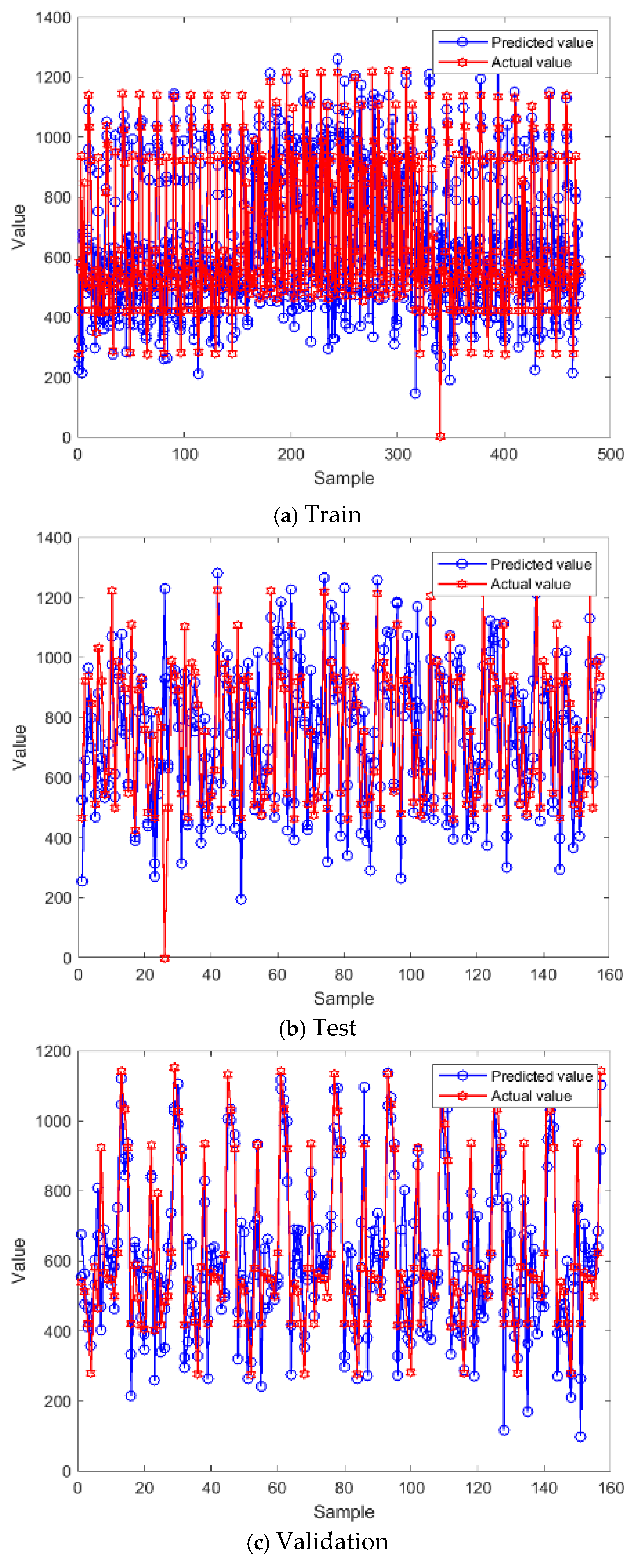
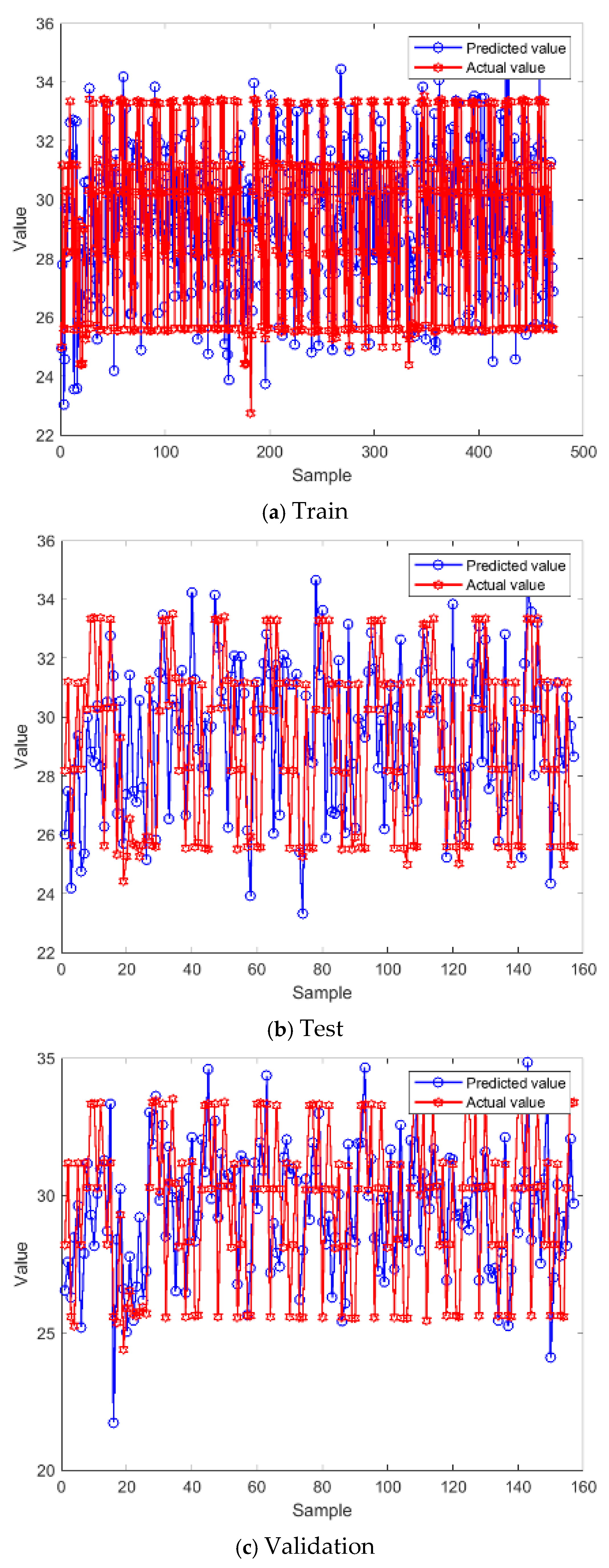
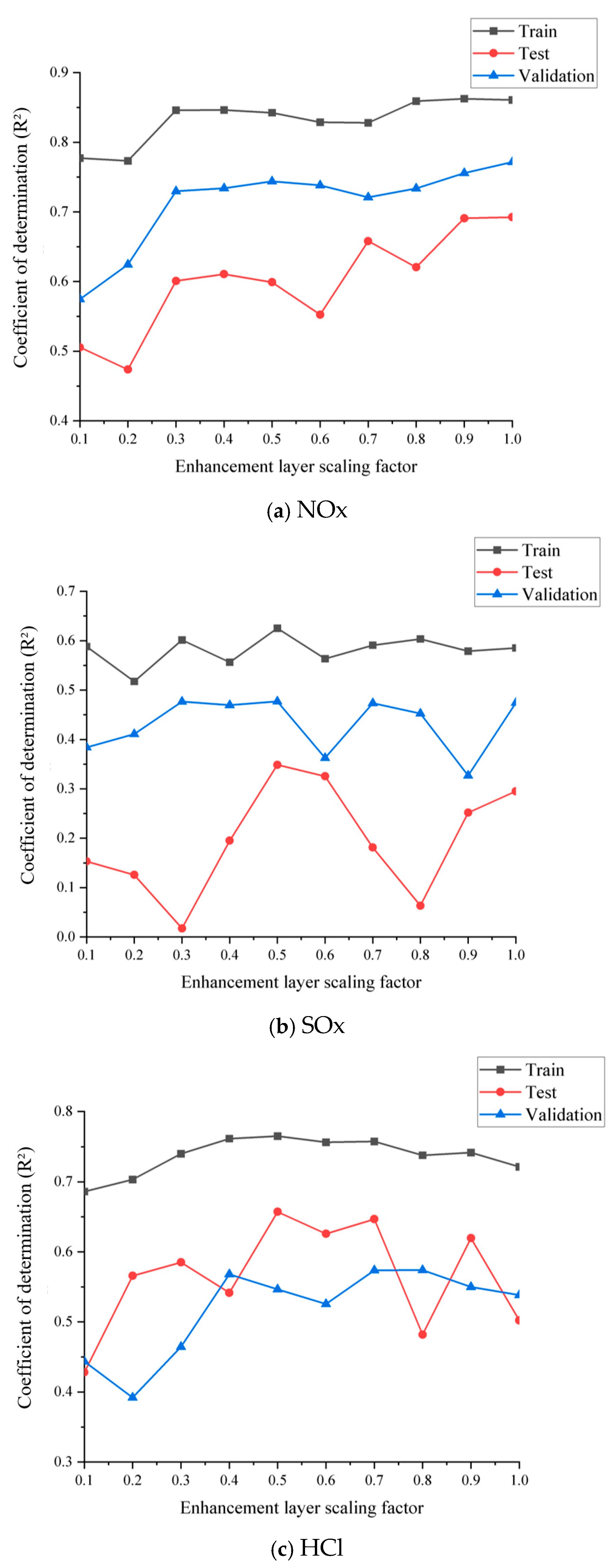
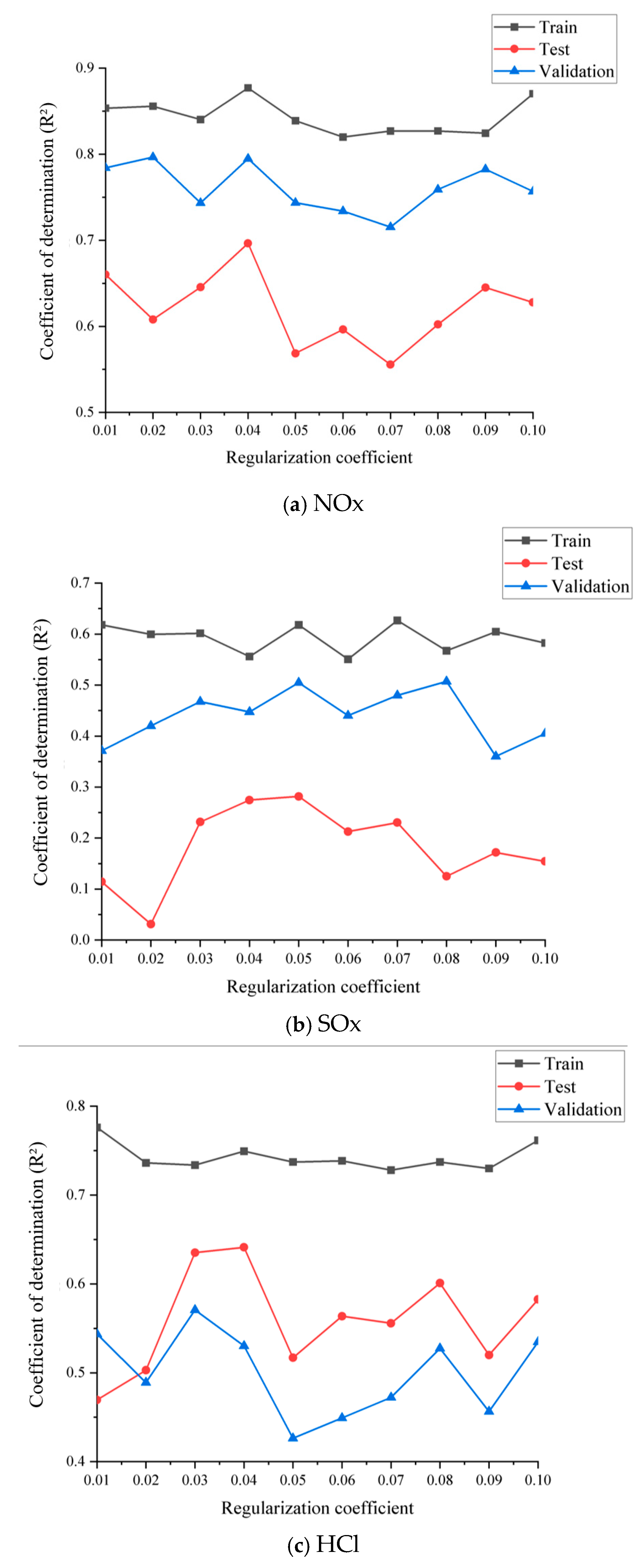
The sample is divided into five parts with equal intervals: parts one, three, and five are the training set, part two is the testing set, and part four is the validation set. The parameters of the IT2FBLS method proposed in this article are set as follows: the number of IT2FBLS subsystems is 100, the number of IT2FBLS subsystem rules is 10, the number of initial augmentation nodes is 25, the mixing weight coefficient is 0.6, the scaling factor of the augmentation layer is 0.4, and the regularization parameter is $4e^{-2}$. The results of the model predictions are shown in Figure 9, Figure 10 and Figure 11.

R² (R-squared, the coefficient of determination) is used as a statistical measure of the goodness of fit of a regression model, with values ranging from 0 to 1. It reflects the proportion of variation in the dependent variable that can be explained by the independent variable. The results are shown in

Table 8. Model prediction indicators.

Data Set	NOx	SOx	HCl
Train	0.83	0.67	0.77
Validation	0.79	0.44	0.55
Test	0.66	0.39	0.56

.

According to Table 8, the NOx model has the best predictive performance and can fit the training data well. The training set of the SOx model is good, but the performance of the validation set and the testing set decreased compared to the training set. The training set of the HCl model is better than that of the SOx model, with stable performance in the testing and validation sets compared to the training set. This indicates that the model has good generalization ability, but there is still room for improvement.

(2)

Method comparison

We chose RF, DT, Gaussian process gegression (GPR), deep neural networks (DNNs), and BPNNs to be compared with the IT2FNN algorithm proposed in this article, and the parameters were set as follows: (1) for RF, the minimum number of samples is 10, the number of RSM feature selections is 10, and the number of decision trees is 50. (2) For DT, the minimum number of samples of the decision tree leaf node is five, the number of RSM feature selections is five, and the number of decision trees is one. (3) For BPNNs, the maximum number of iterations is 1500, the convergence error is 0.001, and the learning rate is 0.01. (4) For GPR, the length scale parameter is 0.6, the amplitude parameter is 0.7, and the standard deviation of noise is 30. (5) For DNNs, the number of fully connected layers is 5, the output channels of the hidden layer are 10, using ReLU as the activation function, the number of iterations is 500, and the batch size is 128. The above method was averaged by running 20 experiments in duplicate under the same conditions, and the statistical results are shown in

Table 9. Statistical results in terms of R² for the comparison experiments.

	NOx			SOx			HCl
	Train	Test	Validation	Train	Test	Validation	Train	Test	Validation
RF	0.44	0.39	0.21	0.35	0.22	0.21	0.39	0.22	0.19
DT	0.42	0.22	0.15	0.33	0.23	0.14	0.22	0.19	0.11
BPNN	0.69	0.32	0.45	0.86	0.35	0.13	0.56	0.55	0.19
GPR	0.80	0.56	0.77	0.66	0.33	0.47	0.78	0.46	0.45
DNN	0.81	0.51	0.86	0.68	0.79	0.86	0.61	0.50	0.47
IT2FBLS	0.82	0.60	0.72	0.64	0.25	0.52	0.78	0.52	0.48

.

Table 9 presents a comparison of the experimental results of different algorithms (RF, DT, BPNN, IT2FBLS, GPR, and DNN) across three models (NOx, SOx, and HCl) and three data subsets (train, test, and validation). For NOx, IT2FBLS showed the highest performance in the train (0.82), test (0.60), and validation (0.72) subsets. In SOx, BPNN had the highest train value (0.86), while IT2FBLS led in the validation subset (0.52), and DT and RF had relatively lower values in most subsets. For HCl, IT2FBLS also demonstrated superior performance, with the highest train (0.78), test (0.52), and validation (0.48) values. Overall, IT2FBLS tended to outperform the other algorithms across different pollutants and data subsets, while DT generally showed lower performance.

(3)

Hyperparameter analysis

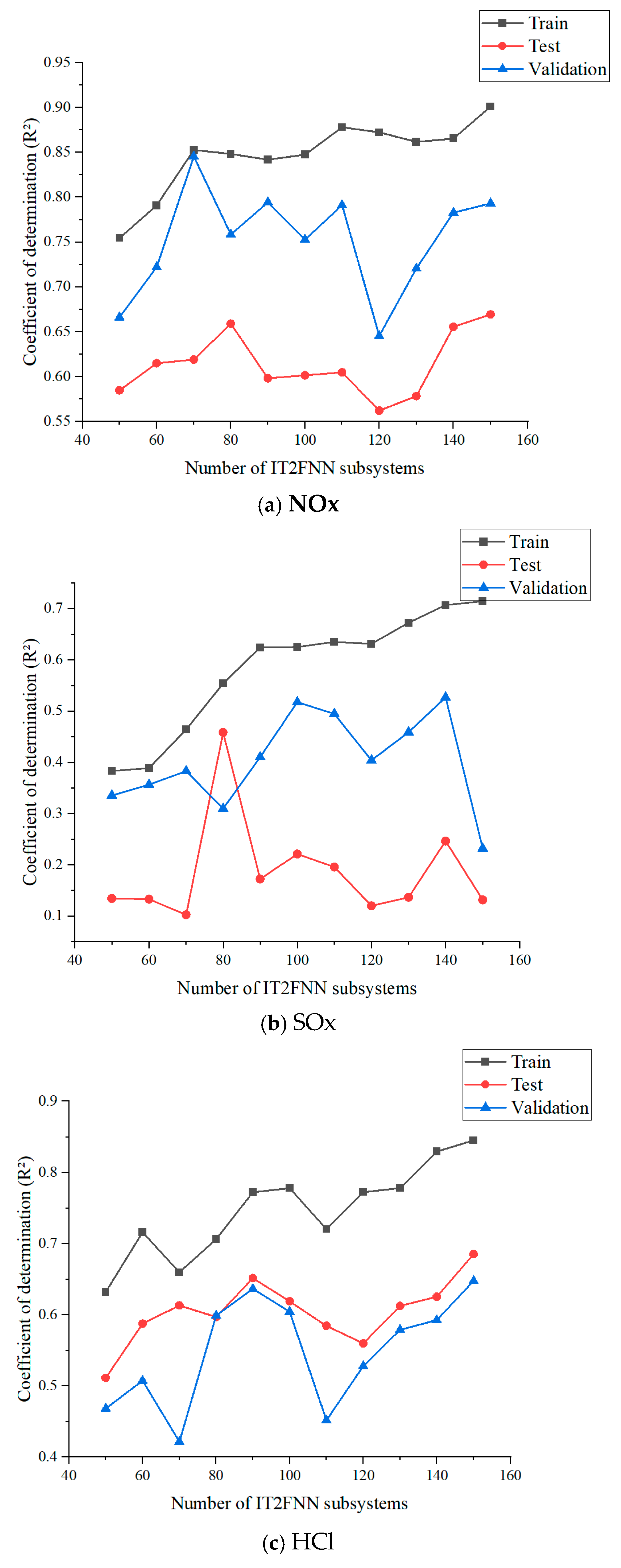
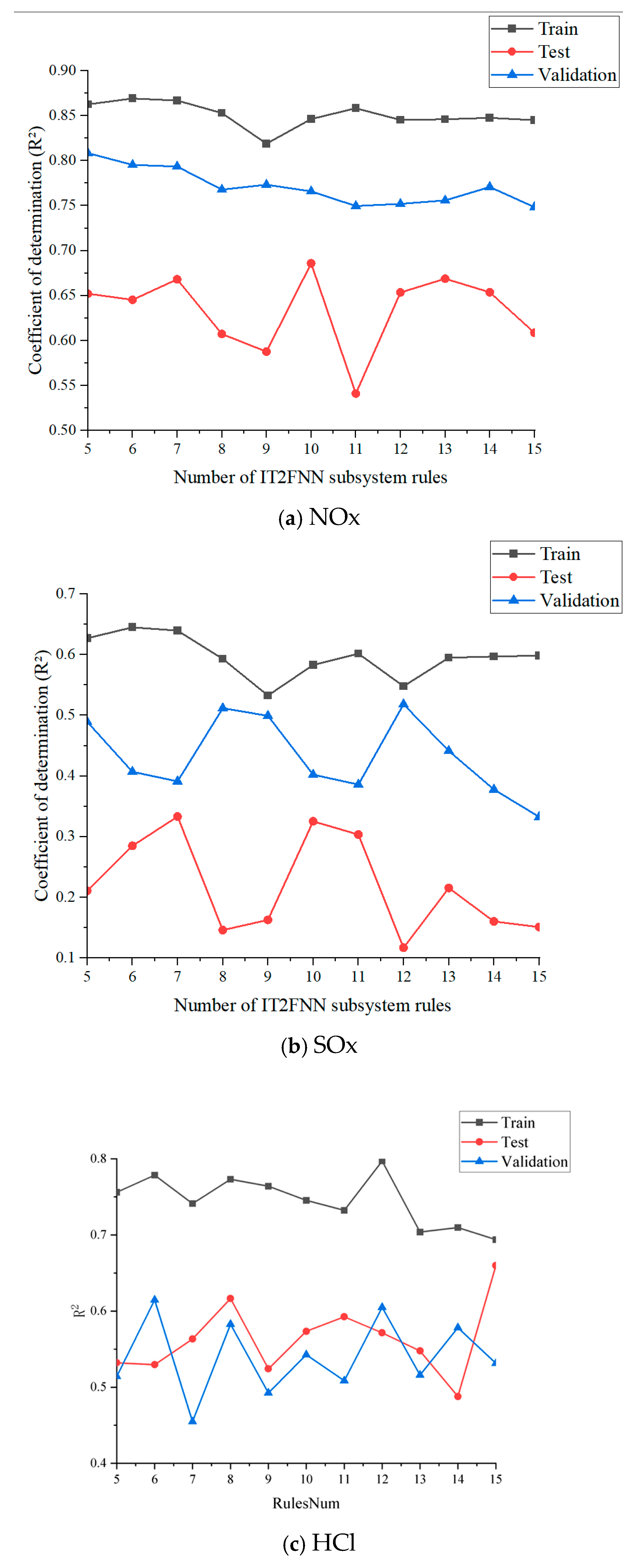
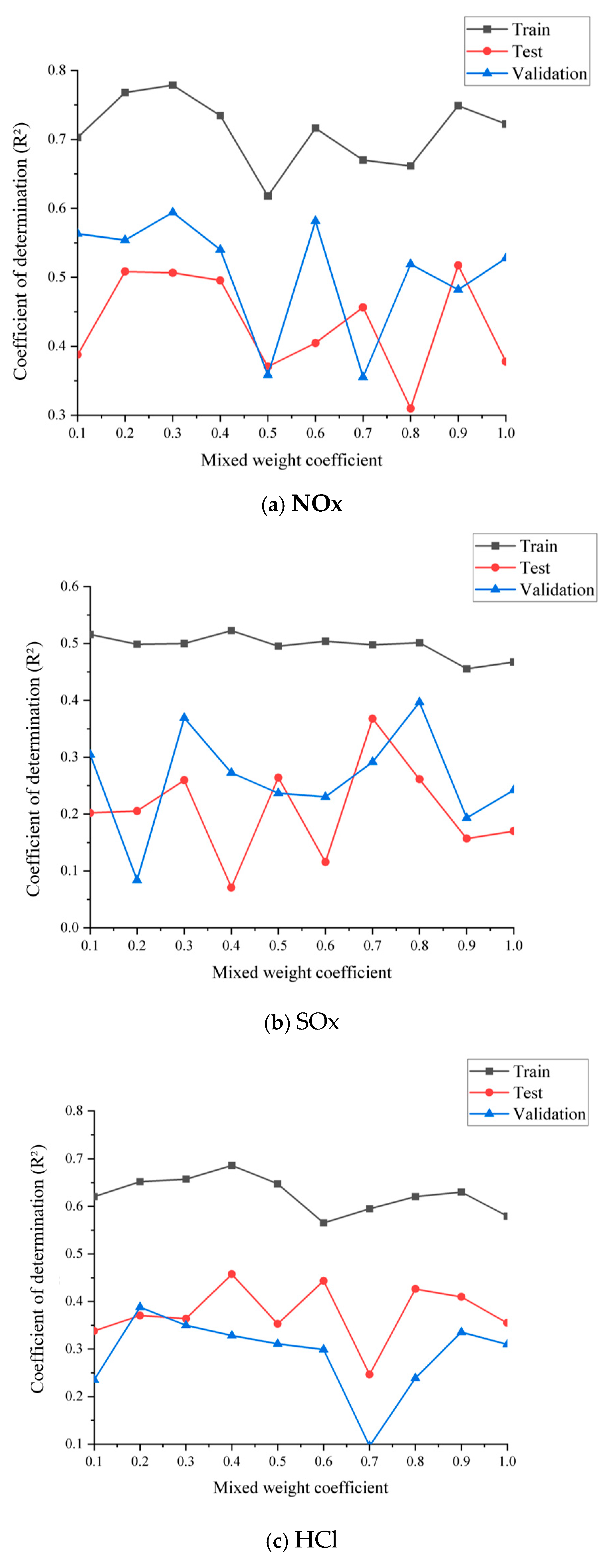
We conducted an analysis on hyperparameters including the number of IT2FBLS subsystems (FuzzyNum), the number of IT2FBLS subsystem rules (RulesNum), the number of initial augmentation nodes (EnhanceNum), the mixing weight coefficient (q), regularization parameters ($\lambda$), and the enhancement layer scaling factor (s). The intervals for each hyperparameter setting are provided in

Table 10. Hyperparameters and their interval setting.

Hyperparameter	Meaning of Hyperparameters	Range
FuzzyNum	Number of IT2FNN subsystems	[40, 160]
RulesNum	Number of IT2FNN subsystem rules	[5, 15]
EnhanceNum	Number of initial augmentation nodes	[5, 55]
q	Mixing weight coefficient	[0.1, 1]
$\lambda$	Regularization parameters	[0.01, 0.1]
s	Enhancement layer scaling factor	[0.1, 1]

. For each hyperparameter, we selected values within a specified range and repeated the experiment 10 times for each value to select the average value.

(A)

Number of IT2FNN subsystems

As can be seen from Figure 12, to NOx model, changes in R² values of the training set, test set, and validation set with the number of IT2FNN subsystems. The R² first increases and then decreases, peaking when the number of subsystems is 80–100. To SOx model, changes in R² values of the training set, test set, and validation set with the number of IT2FNN subsystems. The training set and validation set perform best when the number of subsystems is 80, while the test set shows a gradual downward trend. To HCl model, changes in R² values of the training set, test set, and validation set with the number of IT2FNN subsystems. The training set and validation set reach the highest R² when the number of subsystems is 100, and the test set remains stable at ~0.52.

(B)

Number of IT2FNN subsystem rules

As can be seen from Figure 13, the NO_x model training set and validation set indicators were optimal (≈0.85) when RulesNum = 9, the testing set indicators first increased and then decreased with the increase in the number of rules, and the performance decreased significantly when the number of rules exceeded 11. The SO_x model training set and validation set metrics were stable (≈0.86) when RulesNum = 7–9, and the testing set metrics reached the highest (≈0.55) when the number of rules = 9. The HCl model training set and validation set indicators were the best when RulesNum = 9 (≈0.78), the testing set had little fluctuation with the increase in the number of rules, and the overall performance was the best when the number of rules = 9.

(C)

Mixed weight coefficient

As can be seen from Figure 14, the NOx model training set and validation set metrics reached a peak (≈0.80) at q = 0.4, and the testing set metrics were stable in the range of q = 0.3–0.5 (≈0.60). The SOx model training set and validation set indicators were sensitive to q, the testing set index was the highest (≈0.52) when q = 0.4, and the index decreased significantly after q > 0.6, which may have affected the stability of the model due to weight imbalance. The HCl model training set and validation set indicators were optimal (≈0.78) when q = 0.5, the testing set indicators fluctuated little in the range of q = 0.4–0.6, and the weight coefficients needed to balance the contribution of each subsystem.

(D)

EnhanceNum

As can be seen from Figure 15, the NOx model training set and validation set metrics reached their peak (≈0.85) when EnhanceNum = 20–25, the testing set metrics were optimal (≈0.65) when the number of nodes = 25, and the performance decreased after the number of nodes exceeded 30, which may have introduced noise due to redundant nodes. The SOx model training set and validation set indicators were the best (≈0.86) when EnhanceNum = 20, the testing set indicators first increased and then decreased with the increase in the number of nodes, and the generalization ability was the best when the number of nodes = 20. The HCl model training set and validation set indicators were the highest (≈0.78) when EnhanceNum = 25, the testing set metrics were stable in the interval of node number = 20–25, and the number of nodes was too large to lead to overfitting.

(E)

Enhancement layer scaling factor

As can be seen from Figure 16, the NOx model training set and validation set indicators were optimal (≈0.82) when s = 0.4, and the testing set indicators were stable in the range of s = 0.3–0.5 (≈0.60). The SOx model training set and validation set indicators were the highest (≈0.86) at s = 0.5, and the testing set was the best (≈0.52) at s = 0.4. The HCl model training set and validation set were the best (≈0.78) at s = 0.5, the testing set had a low sensitivity to s, and the comprehensive performance was the best when factor = 0.5.

(F)

Regularization coefficient

As can be seen from Figure 17, the NOx model training set and validation set were optimal (≈0.85) when λ = 0.05, and the testing set was stable in the interval of λ = 0.04–0.06 (≈0.65). The SOx model training set and validation set indicators were the highest (≈0.86) when λ = 0.03, the testing set was the best in the interval λ = 0.03–0.05 (≈0.55), and the regularization intensity should be appropriately controlled to avoid underfitting. The HCl model training set and validation set were the best (≈0.78) when λ = 0.05, the testing set had low sensitivity to λ, and the generalization ability was the best when λ = 0.05.

3.3. Comprehensive Analysis and Discussion

A.

Numerical simulation of benchmark operating conditions for desulfurization and denitrification

The benchmark operating condition is based on a specific single operating condition for testing. The following issues need improvement.

Firstly, the coupled numerical simulation method utilizes the loose coupling characteristics between FLIC and Aspen Plus software programs. The lack of real-time data transmission between software programs is a key drawback, which can be alleviated by standardizing data formats, improving interfaces, and enhancing real-time feedback mechanisms to achieve tight coupling.

Secondly, the simulation system utilizes a hybrid of customized and commercial software. The software belongs to customized software with many ideal conditions, so it may differ from actual operating conditions, while commercial software provides a wider range of applicability and support, but may not fully meet detailed specific MSWI power plant requirements. In the future, integrated professional software in terms of MSWI industrial can be developed through modular design, algorithm optimization, and performance improvement.

Finally, the current simulation system is based on a single actual MSWI power plant. To extend the system to multiple factories, the following factors need to be considered: (1) evaluate the process differences between different factories, and (2) develop a universal management platform that can be applied to multiple MSWI power plants by simply changing the main parameters.

Therefore, a comprehensive desulfurization and denitrification simulation system can be constructed through several key components: (1) develop a simulation software model for the whole MSWI industrial process. The model should consider various production stages and equipment, such as combustion furnaces and gas purification systems. (2) Use fluid dynamics and heat transfer models to simulate the cleaning phase in detail, as this is crucial for the environmental protection objective. (3) Real-time monitoring of the operational status and key parameters of each stage of the process, and adjusting and optimizing the process based on data feedback.

B.

Data acquisition based on a double orthogonal experiment

This study adopted a double orthogonal experimental design to generate virtual mechanism data, selecting 10 influencing factors (7 manipulated variables and 3 non-manipulated variables) and ultimately obtaining 1568 sets of simulation data. The rationality and effectiveness of this design can be illustrated as follows:

Firstly, the adequacy of orthogonality is strictly guaranteed. The experiment was constructed in two stages based on standard orthogonal arrays (OA): the first stage generated 49 cases for 6 factors (with 5 levels each), and the second stage supplemented 32 cases for 5 additional factors (with multiple levels) based on the previous results. In the combined 1568 sets of data, the levels of each factor are evenly distributed, and the correlation coefficient between factors is r < 0.05, indicating no significant collinearity, which meets the core requirement of orthogonality.

Secondly, the coverage of interaction effects focuses on key first-order interactions. Considering the characteristics of the MSWI process, key first-order interactions (e.g., grate speed × feed rate and primary air volume × moisture content) are prioritized. Through the orthogonal array design, each factor level is paired with all levels of other factors (e.g., 6 levels of grate speed and 5 levels of feed rate form 30 combinations). Verification with simulation data shows that these interactions are effectively captured (e.g., the impact of grate speed on NOx concentration is significantly enhanced under high feed rates).

Regarding higher-order interactions, it should be noted that in the MSWI process, higher-order interactions (third-order and above) contribute less to pollutant concentrations (with a variance contribution of <5%), so they are not prioritized in this design. However, partial higher-order effects are indirectly included through large sample sizes (1568 sets) and wide factor ranges (e.g., moisture content: 45–52%; grate speed: 6.0–8.0 m/h). Future studies can combine fractional factorial designs to further strengthen the modeling of higher-order interactions.

As an efficient experimental design method, orthogonal experiments save resources by reasonably selecting factors and levels, systematically analyze influencing factors, and obtaining representative results with fewer experiments. Its advantages include saving experimental costs, a clear system structure, ease of analysis, and identification of main factors. However, orthogonal experiments also have limitations, such as being unsuitable for complex interaction systems, limited level settings, and complex experimental designs. Therefore, other experimental design methods (e.g., the supersaturated Latin square design) may be considered in the future, which can explore more factor combinations with fewer experiments while improving the differentiation between factor levels.

C.

Mechanism model construction module based on an improved IT2FBLS algorithm perspective

Although the improved IT2FBLS algorithm has demonstrated effective modeling capabilities for desulfurization and denitrification pollutant concentrations in this study, there is still room for optimization and future research directions as follows.

(1)

Multi-source data fusion: The current model relies on virtual simulation data, and in the future, it can be combined with real-time monitoring data from actual MSWI power plants (such as online flue gas analyzer data) to enhance the adaptability of the model to complex industrial environments through data fusion technology, especially for robustness against non-Gaussian noise and dynamic oeprating conditions.

(2)

Dynamic modeling capability: Existing models are designed based on steady-state operating conditions and require the introduction of time series analysis (such as recursive mechanisms or dynamic fuzzy rules) to capture the time-varying characteristics caused by fuel component fluctuations, equipment aging, and other factors during the incineration process, in order to achieve dynamic pollutant concentration prediction.

(3)

Algorithm lightweight and deployment: The multi-layer structure of IT2FBLS may face computational resource limitations in industrial edge computing devices. Lightweight versions can be developed through parameter pruning, hardware acceleration (such as FPGA/ASIC), or transfer learning to promote the engineering application of the model in real-time control scenarios.

(4)

Enhanced interpretability: Combining fuzzy rule visualization techniques (such as rule heat maps and feature importance analysis), analyzing the response mechanism of the model to key operating variables (such as urea flow rate and lime dosage), and providing transparent decision support for process optimization.

D.

sensitivity analysis

The results of the orthogonal experiments were subjected to sensitivity analysis, as shown in

Table 11. Sensitivity analysis results.

Factors	With HCl (%)	With SO2 (%)	With NOx (%)
Grate speed	5.84	4.24	0.03
Feed rate	0.57	0.71	0.03
Primary air volume	1.11	1.38	0.03
Moisture content	0.64	0.95	0.01
Particle size	0.63	0.88	0.01
Particle mixing coefficient	0.39	0.79	0.01
Secondary air volume	38.53	53.06	2.92
Secondary air temperature	7.84	7.02	3.53
Urea feeding flow rate	7.33	5.33	85.01
Lime feeding amount	55.5	45.34	5.16

.

(1)

Impact on HCl concentration

Dominant factors: Secondary air volume (38.53%) and lime feeding amount (55.5%) are the key determinants of HCl concentration, collectively contributing over 90%. The lime feeding amount, with the highest contribution, plays a decisive role in HCl removal as a desulfurization and dechlorination agent. Secondary air volume significantly affects HCl generation and removal by regulating oxygen supply and reaction conditions in the furnace.

Secondary factors: Secondary air temperature (7.84%) and urea feeding flow rate (7.33%) have moderate impacts, indirectly influencing HCl concentration by altering reaction temperatures and chemical environments in the furnace.

Minor factors: Grate speed (5.84%), primary air volume (1.11%), moisture content (0.64%), particle size (0.63%), feed rate (0.57%), and particle mixing coefficient (0.39%) contribute less than 6%, exerting weak effects on HCl fluctuations.

(2)

Impact on SO₂ concentration

Dominant factors: Secondary air volume (53.06%) and lime feeding amount (45.34%) are the core factors controlling SO₂ concentration, with a combined contribution approaching 99%. Secondary air volume determines SO₂ generation by influencing combustion efficiency and oxygen levels, while the lime feeding amount directly reduces SO₂ emissions through desulfurization reactions, collectively dominating SO₂ levels.

Secondary factors: Secondary air temperature (7.02%) and urea feeding flow rate (5.33%) have relatively minor contributions (<8%), playing limited roles in SO₂ regulation.

Minor factors: Grate speed (4.24%), primary air volume (1.38%), moisture content (0.95%), particle size (0.88%), feed rate (0.71%), and particle mixing coefficient (0.79%) contribute less than 5%, with insignificant impacts on SO₂ concentration.

(3)

Impact on NOx concentration

Dominant factor: Urea feeding flow rate (85.01%) is the decisive factor affecting NOx concentration. As a denitrification agent, its flow rate directly determines the efficiency of the SNCR denitrification reaction, dominating NOx removal.

Secondary factors: Lime feeding amount (5.16%), secondary air temperature (3.53%), and secondary air volume (2.92%) contribute moderately (<6%), indirectly influencing NOx generation and reduction by altering furnace temperature and reaction conditions.

Negligible factors: Grate speed (0.03%), feed rate (0.03%), primary air volume (0.03%), moisture content (0.01%), particle size (0.01%), and particle mixing coefficient (0.01%) contribute almost nothing, with minimal to no impact on NOx fluctuations.

(4)

Comprehensive conclusions

Sensitive factors vary significantly among pollutants: NOx concentration is primarily controlled by the urea feeding flow rate, while SO₂ and HCl concentrations are dominated by the lime feeding amount and secondary air volume.

Manipulated variables (e.g., secondary air volume, lime feeding amount, and urea feeding flow rate) exert far greater influences on pollutant concentrations than non-manipulated variables (e.g., moisture content and particle size), providing clear directions for parameter optimization in industrial pollutant reduction.

Secondary air volume affects all three pollutants, emerging as a key factor for coordinating desulfurization, denitrification, and dechlorination efficiency.

3.4. Comparison with Similar Published Works

To contextualize the novelty and performance of the proposed approach, this section compares the current study with relevant literature focusing on MSWI pollutant modeling, numerical simulation, and data-driven methods.

Existing studies on MSWI numerical simulation primarily focus on single-process modeling or specific pollutants. For example, Zhuang et al. [8] developed a grate furnace combustion model using FLIC to analyze temperature distribution and dioxin formation, but did not integrate desulfurization/denitrification processes. Chen et al. [20] combined computational fluid dynamics (CFD) with deep forest regression to model furnace temperature fields, but their work excluded pollutant reduction mechanisms. In contrast, the present study constructs a coupled FLIC-Aspen Plus model covering the entire life cycle of desulfurization and denitrification, from solid-phase combustion to flue gas purification. This multi-software integration enables simultaneous simulation of nitrogen oxides (NOx), sulfur oxides (SOx), and hydrogen chloride (HCl) dynamics, which has not been reported in prior MSWI research. The model’s prediction of post-treatment pollutant concentrations (NOx: 67.56 mg/m³, SOx: 11.77 mg/m³, and HCl: 5.4 mg/m³) aligns with industrial benchmarks (e.g., GB 18485-2014 standards) and shows better agreement with on-site data (Table 6) than standalone FLIC or Aspen Plus models in previous studies [10,12].

AI-based models for MSWI pollutants often rely on traditional algorithms with limited uncertainty handling. For instance, Chen et al. [20] used deep forest regression to predict temperature fields (R² ≈ 0.75) but did not extend to pollutant concentrations. Xu et al. [19] combined CFD with neural networks for solid oxide fuel cell optimization, achieving R² ≈ 0.80 for efficiency but not pollutant reduction. The proposed improved interval type-II fuzzy broad learning system (IT2FBLS) outperforms conventional methods (random forests, decision trees, back propagation neural networks) in predicting NOx (test R² = 0.66), SOx (0.39), and HCl (0.56) (Table 9). Its integration of interval type-II fuzzy logic and incremental learning addresses uncertainties in waste composition and combustion conditions, a capability lacking in most data-driven MSWI models. This performance surpasses the NOx prediction accuracy (R² ≈ 0.50) reported in Hu et al. [12] using CFD alone and the SO₂ modeling (R² ≈ 0.40) in Zhong et al. [15] for wet desulfurization systems.

4. Conclusions

This study proposes a whole life cycle modeling method that integrates numerical simulation and an improved intelligent algorithm (interval type-II fuzzy broad learning system) to address the challenges of understanding the formation mechanisms and controlling desulfurization and denitrification pollutants in municipal solid waste incineration. The main contributions are as follows. (1) Coupled numerical simulation model: By integrating FLIC and Aspen Plus, the model quantifies pollutant dynamics across key stages. Under benchmark operating conditions, after desulfurization and denitrification, concentrations of NOx, HCl, and SOx are reduced to 67.56 mg/m³, 5.4 mg/m³, and 11.77 mg/m³, respectively, aligning with on-site monitoring data. (2) Double orthogonal experimental data: A double orthogonal design with 10 factors (7 operating variables and 3 non-operating variables) generated 1568 sets of virtual data. The sufficiency of this dataset is justified in terms of coverage and statistical robustness criteria. For the former one, it exceeds sample sizes in comparable studies, ensuring comprehensive sampling of factor ranges (e.g., grate speed: 6.0–8.0 m/h and moisture content: 45–52%). For the latter, the coefficient of variation for pollutant predictions stabilizes below 5% with >1200 samples, indicating minimal improvement from additional data. This dataset captures key first-order interactions (e.g., grate speed × feed rate) critical to MSWI processes, with higher-order interactions contributing <5% to total variance. (3) IT2FBLS mechanism model: The improved interval type-II fuzzy broad learning system achieves quantifiable predictive performance. For NOx, SOx, and HCl, the R² values for the training and testing sets are 0.83 and 0.66, 0.67 and 0.39, and 0.77 and 0.56, respectively.

This model provides data support for optimizing process parameters (e.g., the negative correlation between urea flow rate and nitrogen oxide concentration, and the nonlinear suppression of sulfur oxides by lime dosage) and lays the foundation for subsequent intelligent optimization control, which is conducive to achieving synergistic goals of pollutant reduction and energy efficiency improvement. Additionally, this study analyzes how various process parameters influence pollutant concentrations, offering a reference for continuously optimizing the municipal solid waste incineration process to achieve energy conservation and emission reduction.

Future efforts will focus on three strategic directions to enhance the practical applicability and realism of the proposed framework. (1) Integration of hybrid data streams: Robust integration of real-time industrial monitoring data with virtual simulation data will improve the model’s adaptability and predictive accuracy under dynamic operating conditions, particularly in response to unforeseen events such as sudden changes in waste composition or operational parameters. This integration will bridge the gap between theoretical modeling and real-world variability. (2) Development of a lightweight IT2FBLS system: Optimization of the IT2FBLS algorithm will yield a more lightweight, resource-efficient version, facilitating seamless deployment and efficient operation in real-time monitoring and control environments within industrial settings. (3) Advanced 3D visualization simulation: Construction of sophisticated 3D simulation models will enable visualization of temperature fields and gas concentration fields within the incinerator furnace, offering insights into the complex spatial and temporal dynamics of the incineration process to aid in optimization and troubleshooting.

Furthermore, acknowledging inherent uncertainties in complex industrial processes, the IT2FBLS algorithm is designed to handle such variability. Systematic uncertainty analysis will be conducted following methodologies exemplified in relevant literature to quantify and manage the model’s predictive robustness [29]. These efforts will ensure the research evolves toward highly practical applications in municipal solid waste incineration management.

References

1. Tang, J.; Xia, H.; Yu, W.; Qiao, J. Research status and prospects of intelligent optimization control for municipal solid waste incineration process. Acta Autom. Sin. 2023, 49, 2019–2059. [Google Scholar]
2. Liu, B.; Han, Z.; Li, J.; Yan, B. Comprehensive evaluation of municipal solid waste power generation and carbon emission potential in Tianjin based on Grey Relation Analysis and Long Short Term Memory. Process Saf. Environ. Prot. 2022, 168, 918–927. [Google Scholar] [CrossRef]
3. Teng, F.; Wang, Z.; Ren, K.; Liu, S.; Ding, H. Analysis of composition characteristics and treatment techniques of municipal solid waste incineration fly ash in China. J. Environ. Manag. 2024, 357, 120783. [Google Scholar] [CrossRef] [PubMed]
4. Qiao, J. Intelligent Optimization Control of Municipal Solid Waste Incineration Process Eng; Chemical Industry Press Co., Ltd.: Beijing, China, 2023. [Google Scholar]
5. Zhu, Y.; Liu, L. Shipping Emissions and Air Pollution: Latest Methodological Developments and Applications. Atmosphere 2023, 14, 1312. [Google Scholar] [CrossRef]
6. Evans, C.D.; Monteith, D.T.; Fowler, D. Hydrochloric Acid: An Overlooked Driver of Environmental Change. Environ. Sci. Technol. 2011, 45, 1887–1894. [Google Scholar] [CrossRef] [PubMed]
7. Luo, B.; Su, Y.; Ding, X.; Chen, Y.; Liu, C. Modulation of initial CaO/Al2O3 and SiO2/Al2O3 ratios on the properties of slag/fly ash-based geopolymer stabilized clay: Synergistic effects and stabilization mechanism. Mater. Today Commun. 2025, 47, 113295. [Google Scholar] [CrossRef]
8. Quan, L.M.; Kamyab, H.; Yuzir, A.; Ashokkumar, V.; Hosseini, S.E.; Balasubramanian, B.; Kirpichnikova, I. Review of the application of gasification and combustion technology and waste-to-energy technologies in sewage sludge treatment. Fuel 2022, 316, 123199. [Google Scholar] [CrossRef]
9. Sun, Y.; Qin, Z.; Tang, Y.; Huang, T.; Ding, S.; Ma, X. Techno-Environmental-Economic Evaluation on Municipal Solid Waste (MSW) to Power/Fuel by Gasification-Based and Incineration-Based Routes. J. Environ. Chem. Eng. 2021, 9, 106108. [Google Scholar] [CrossRef]
10. Chen, J.K.; Tang, J.; Xia, H.; Qiao, J. Numerical simulation of dioxin emission concentration in grate furnace incineration processes for municipal solid waste. Chem. Ind. Eng. Prog. 2023, 42, 1061–1072. [Google Scholar]
11. Xia, H.; Tang, J.; Aljerf, L.; Chen, J.K. Unveiling dioxin dynamics: A whole-process simulation study of municipal solid waste incineration. Sci. Total Environ. 2024, 954, 176241. [Google Scholar] [CrossRef]
12. Hu, Z.; Jiang, E.; Ma, X. Numerical simulation on NOx emissions in a municipal solid waste incinerator. J. Clean. Prod. 2019, 233, 650–664. [Google Scholar] [CrossRef]
13. Liu, J.; Zhu, Y.; Zhou, H. Numerical simulation study on combustion characteristics and NOx emission of COREX gas swirl burner and boiler. Fuel 2023, 352, 129128. [Google Scholar] [CrossRef]
14. Tang, H.; Liu, Z.; Han, X.; Shen, X.; Liu, Y.; Wang, S.; Xu, Z. Experimental study on combustion characteristics of a 40 MW pulverized coal boiler based on a new low NOx burner with preheating function. Energy 2024, 305, 132319. [Google Scholar] [CrossRef]
15. Zhong, Y.; Gao, X.; Huo, W.; Luo, Z.-Y.; Ni, M.-J.; Cen, K.-F. A model for performance optimization of wet flue gas desulfurization systems of power plants. Fuel Process. Technol. 2008, 89, 1025–1032. [Google Scholar] [CrossRef]
16. Xu, B.; Chen, P. Enhancing SO2 emission concentration prediction in ammonia flue gas desulfurization systems through continual learning. J. Environ. Chem. Eng. 2025, 13, 116248. [Google Scholar] [CrossRef]
17. Tao, L.; Wu, H.; Wang, J.; Li, B.; Wang, X.; Ning, P. Removal of SO2 from flue gas using Bayer red mud: Influence factors and mechanism. J. Cent. South Univ. 2019, 26, 467–478. [Google Scholar] [CrossRef]
18. Zhou, C.; He, Y.; Liu, J.; Yang, F.; Min, X.; Jing, Y. Mechanism-data hybrid driven model building method for RH decarbonization. China Metall. 2023, 33, 54–60. [Google Scholar]
19. Xu, G.; Yu, Z.; Xia, L.; Wang, C.; Ji, S. Performance improvement of solid oxide fuel cells by combining three-dimensional CFD modeling, artificial neural network and genetic algorithm. Energy Convers. Manag. 2022, 268, 116026. [Google Scholar] [CrossRef]
20. Zhou, Y.; Aslanidou, I.; Karlsson, M.; Kyprianidis, K. An explainable AI model for power plant NOx emission control. Energy AI 2024, 15, 100326. [Google Scholar] [CrossRef]
21. Fei, J.; Wang, Z.; Liang, X.; Feng, Z.; Xue, Y. Fractional sliding-mode control for microgyroscope based on multilayer recurrent fuzzy neural network. IEEE Trans. Fuzzy Syst. 2021, 30, 1712–1721. [Google Scholar] [CrossRef]
22. Liang, Q.; Mendel, J.M. Interval type-2 fuzzy logic systems: Theory and design. IEEE Trans. Fuzzy Syst. 2000, 8, 535–550. [Google Scholar] [CrossRef] [PubMed]
23. Chen, P.C.L.; Liu, Z. Broad learning system: An effective and efficient incremental learning system without the need for deep architecture. IEEE Trans. Neural Netw. Learn. Syst. 2017, 29, 10–24. [Google Scholar] [CrossRef]
24. Yang, Y.B.; Sharifi, V.N.; Swithenbank, J. Converting moving-grate incineration from combustion to gasification—Numerical simulation of the burning characteristics. Waste Manag. 2007, 27, 645–655. [Google Scholar] [CrossRef]
25. Dong, J.; Tang, Y.; Hu, Y.; Wang, S.; Zhou, Z.; Shi, Y.; Liu, C.; Wang, F. Effect of CaO addition on fast pyrolysis behavior of solid waste components using Py GC/MS. J. Anal. Appl. Pyrolysis 2025, 188, 107055. [Google Scholar] [CrossRef]
26. Illan-Gomez, M.J.; Linares-Solano, A.; Radovic, L.R.; de Lecea, C.S.-M. NO reduction by activated carbons. 4. Catalysis by calcium. Energy Fuels 1995, 9, 112–118. [Google Scholar] [CrossRef]
27. Ding, X.-H.; Luo, B.; Zhou, H.-T.; Chen, Y.-H. Generalized solutions for advection–dispersion transport equations subject to time- and space-dependent internal and boundary sources. Comput. Geotech. 2025, 178, 106944. [Google Scholar] [CrossRef]
28. Tsai, S.H.; Chen, Y.W. A novel interval type-2 fuzzy system identification method based on the modified fuzzy c-regression model. IEEE Trans. Cybern. 2021, 52, 9834–9845. [Google Scholar] [CrossRef]
29. Chen, Y.; Zhang, L.; Xu, L.; Zhou, S.; Luo, B.; Ding, K. In-situ investigation on dynamic response of highway transition section with foamed concrete. Earthq. Eng. Eng. Vib. 2025, 24, 547–563. [Google Scholar] [CrossRef]
Figure 1. MSWI process flow in terms of desulfurization and denitrification.
Sustainability 17 10097 g001
Figure 2. Structure of·the edge verification platform of an actual MSWI power plant.
Sustainability 17 10097 g002
Figure 3. Modeling strategy.
Sustainability 17 10097 g003
Figure 4. Numerical simulation model of gas-phase combustion based on Aspen Plus.
Sustainability 17 10097 g004
Figure 5. Flowchart of the modeling strategy.
Sustainability 17 10097 g005
Figure 6. Distribution of gas-phase temperature during solid-phase combustion on the grate.
Sustainability 17 10097 g006
Figure 7. Results of the distribution of gas-phase components on the grate.
Sustainability 17 10097 g007
Figure 8. Concentrations of NOx, HCl, and SOx at different process zones under benchmark operating conditions.
Sustainability 17 10097 g008
Figure 9. NOx model prediction curves.
Sustainability 17 10097 g009
Figure 10. SOx model prediction curves.
Sustainability 17 10097 g010
Figure 11. HCl model prediction curves.
Sustainability 17 10097 g011
Figure 12. Analysis of the impact of the number of IT2FNN subsystems on model performance.
Sustainability 17 10097 g012
Figure 13. Analysis of the impact of the number of IT2FNN subsystem rules on model performance.
Sustainability 17 10097 g013
Figure 14. Analysis of the impact of the mixing weight coefficient on model performance.
Sustainability 17 10097 g014
Figure 15. Analysis of the impact of the number of initial augmentation nodes on model performance.
Sustainability 17 10097 g015
Figure 16. Analysis of the impact of enhancement layer scaling factor on model performance.
Sustainability 17 10097 g016
Figure 17. Analysis of the impact of regularization coefficient on model performance.
Sustainability 17 10097 g017