Long-Term Traffic Flow Prediction for Highways Based on STLLformer Model

Abstract

Long-term traffic flow prediction (LTFP) is crucial for intelligent transportation systems but remains challenging due to complex spatiotemporal dependencies and multi-scale temporal patterns. While recent models like Autoformer have introduced decomposition techniques, they often lack tailored mechanisms for traffic data’s unique characteristics, such as strong periodicity and long-range spatial correlations. To address this gap, we propose STLLformer, a novel spatiotemporal Transformer that establishes a seasonal-dominated, multi-component collaborative forecasting paradigm. Unlike existing approaches that merely combine decomposition with graph networks, STLLformer features: (1) a dedicated encoder–decoder architecture for separate yet synergistic modeling of trend, seasonal, and residual components; (2) a seasonal-driven autocorrelation mechanism that purely captures cyclical patterns by filtering out trend and noise interference; and (3) a low-rank graph convolutional module specifically designed to capture dynamic, long-range spatial dependencies in road networks. Experiments on two real-world traffic datasets (PEMSD8 and HHY) demonstrate that STLLformer outperforms strong baseline methods (including LSTGCN, LSTM, and ARIMA), achieving an average improvement of over 10% in MAE and RMSE (e.g., on PEMSD8 for 6-h prediction, MAE drops from 36.87 to 30.34), with statistical significance (p < 0.01). This work provides a more refined and effective decomposition-fusion solution for traffic forecasting, which holds practical promise for enhancing urban traffic management and alleviating congestion.

1. Introduction

Long-term traffic flow prediction (LTFP) on highways is a crucial task in intelligent transportation systems (ITS), enabling proactive traffic management and sustainable urban planning [1]. Accurately forecasting traffic conditions hours or days ahead is essential for applications like congestion mitigation, dynamic route guidance, and infrastructure planning [2]. Despite its importance, LTFP remains challenging due to the complex spatiotemporal dependencies and multi-scale temporal patterns inherent in traffic data [3].

Highway traffic flow exhibits complex spatiotemporal characteristics. Temporally, it shows strong seasonality driven by commuting patterns [4]. Spatially, flow variations across monitoring points are influenced by network topology and upstream/downstream conditions [5]. These dependencies are the core mechanisms of traffic propagation and key to accurate forecasting.

1.1. Related Work and Challenges

Current research on LTFP has evolved through statistical methods, machine learning, to deep learning paradigms. Traditional statistical models such as ARIMA [6] perform well in modeling short-term trends but struggle with long-term nonlinear fluctuations [7,8]. Machine learning methods like SVM [9] have enhanced fitting capabilities but still fall short in capturing complex spatiotemporal dependencies. Recently, deep learning methods have gained traction due to their powerful feature representation and end-to-end modeling capabilities. Models such as LSTM [10] and GANs [11] have shown promising results across various scenarios. The integration of attention mechanisms has further improved the modeling of long-range dependencies [12].

To strengthen spatial modeling, graph convolutional networks (GCNs) and their derivatives have been widely used to represent road network structures [13]. Approaches such as DCRNN [14], STGCN [15], and ASTGCN [16] jointly extract spatial and temporal features through graph convolution and sequential modeling. Advanced models like STSGCN [17] achieve synchronous spatiotemporal modeling, while dynamic graph convolutional networks [18] incorporate spatiotemporal feature extraction modules to model dependencies. Meanwhile, Transformer-based [19] and self-supervised learning models [20] have also shown promise in modeling long-term memory and spatiotemporal heterogeneity.

Recently, several studies have integrated series decomposition into deep spatiotemporal forecasting models. For instance, Autoformer [21] introduced a decomposition architecture with an auto-correlation mechanism to capture long-term temporal dependencies, while ACNet [22] explored adaptive correlation for time series forecasting. These works provide valuable insights. However, applying them directly to traffic flow forecasting poses limitations: Firstly, they typically process the decomposed subsequences in a mixed manner, lacking dedicated modeling strategies for the trend, seasonal, and residual components, which possess distinct physical meanings [23]. Secondly, their primary focus lies on temporal modeling, and their approach to spatial dependency capture often relies on standard graph convolutional networks, which struggle to effectively model the prevalent long-range spatial interactions in road networks [24].

Despite these advances, LTFP still faces three core challenges when applying existing models, summarized in Table 1:

(C1) Monolithic Sequence Modeling: Most existing forecasting models tend to treat traffic flow time series as holistic entities, without fully leveraging their internal structural differences [25]. This limits their ability to respond accurately to complex and dynamically changing traffic patterns.

(C2) Inadequate Seasonal Modeling: Although seasonality is recognized, most modeling approaches rely on static weighting or embedding schemes, lacking dynamic mechanisms for modeling seasonal structures [26].

(C3) Limited Long-range Spatial Modeling: Existing spatial modeling methods typically construct graph structures based on static adjacency matrices, which are insufficient for capturing the non-uniform and dynamic dependencies among distant nodes in road networks [27].

Table 1. Methodological comparison of spatiotemporal forecasting models.

Model	Temporal Modeling	Spatial Modeling	Decomposition Strategy	Key Limitation
STGCN [15]	Gated CNN	GCN	No	Monolithic processing (C1)
LSTGCN [28]	GRU	GCN	No	Monolithic processing (C1)
Informer [6]	ProbSparse Attention	Basic/None	No	Lacks spatial modeling & component heterogeneity (C1, C3)
Autoformer [21]	Auto-Correlation	Basic/None	Series Decomposition Block	Mixed component processing (C2); Lacks long-range spatial modeling (C3)
STLLformer (Ours)	Seasonal-driven Auto-Correlation	Low-rank GCN	STL + Component-specific Modeling	Designed to address C1, C2, C3

Table 1. Methodological comparison of spatiotemporal forecasting models.

Model	Temporal Modeling	Spatial Modeling	Decomposition Strategy	Key Limitation
STGCN [15]	Gated CNN	GCN	No	Monolithic processing (C1)
LSTGCN [28]	GRU	GCN	No	Monolithic processing (C1)
Informer [6]	ProbSparse Attention	Basic/None	No	Lacks spatial modeling & component heterogeneity (C1, C3)
Autoformer [21]	Auto-Correlation	Basic/None	Series Decomposition Block	Mixed component processing (C2); Lacks long-range spatial modeling (C3)
STLLformer (Ours)	Seasonal-driven Auto-Correlation	Low-rank GCN	STL + Component-specific Modeling	Designed to address C1, C2, C3

As shown in Table 1, while Autoformer introduces decomposition, its architecture is not specifically designed for traffic data’s unique characteristics. It processes decomposed components through a unified block, potentially failing to fully leverage their distinct properties (C2), and its spatial modeling capability remains underdeveloped (C3).

1.2. Our Contributions

Different from these models, our proposed STLLformer implements a seasonal-dominated, multi-component collaborative modeling paradigm. The main contributions are:

• A Component-specific Encoder–Decoder Architecture. We design a novel architecture where the seasonal component is processed separately by the encoder, and all three components (trend, seasonal, residual) are modeled in parallel within the decoder [29]. This enables targeted feature extraction for each component’s unique characteristics, directly addressing C1.
• A Seasonal-driven Autocorrelation Mechanism. This mechanism operates purely on the seasonal subsequence, filtering out interference from trend and noise to provide dynamic and precise capture of cyclical traffic patterns [30], thereby effectively addressing C2.
• A Low-rank Graph Convolutional Network (LGCN). This module performs low-dimensional reconstruction and dynamic filtering of the graph structure, explicitly enhancing multi-scale spatial node interaction and the modeling of long-range dependencies [31,32,33], filling a key technical gap (C3).

The remainder of this paper is organized as follows: Section 2 describes the STLLformer architecture and core modules; Section 3 presents experimental results and analysis; Section 4 concludes with the discussion and future work.

2. Methodology

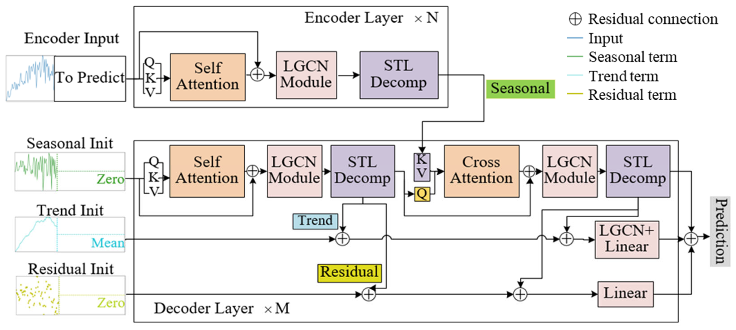
To enhance the modeling capability of temporal structures and spatial dependencies in long-term traffic flow prediction, this paper proposes STLLformer, a novel prediction model based on temporal decomposition and graph spatio-temporal modeling. The model adopts a Transformer encoder–decoder architecture, integrating STL temporal decomposition, autocorrelation mechanisms, time delay aggregation, and graph convolutional structures to achieve multi-dimensional modeling of trend, seasonal, and residual fluctuations in traffic flow data. This design directly addresses the challenges of monolithic sequence modeling (C1), inadequate seasonal modeling (C2), and limited long-range spatial modeling (C3). Figure 1 illustrates the overall architecture and information flow of the proposed model.

Figure 1. Architecture of the long-term spatiotemporal prediction network based on low-rank graph and STL decomposition.

At the input stage of the encoder–decoder architecture, we incorporate an STL temporal decomposition mechanism that splits the original traffic flow sequence into three components—trend, seasonal and residual terms—enabling separate modeling of long-term trends, seasonal variations and short-term disturbances. The seasonal component serves as the primary input to the encoder, where the multi-head autocorrelation mechanism first identifies strongly correlated temporal positions exhibiting seasonal, and then the time delay aggregation module performs feature fusion, while a graph convolutional network is incorporated to model spatial structural information. In the decoder, the trend, seasonal, and residual terms are modeled separately. The seasonal component additionally incorporates encoder outputs through cross-attention to enable information interaction. Finally, the predictions of the three components are aggregated at the output layer to generate the final traffic flow prediction. This architecture effectively models multi-scale temporal features and complex spatial dependencies in traffic data, improving both prediction accuracy and model generalization capability.

2.1. STL Decomposition Module

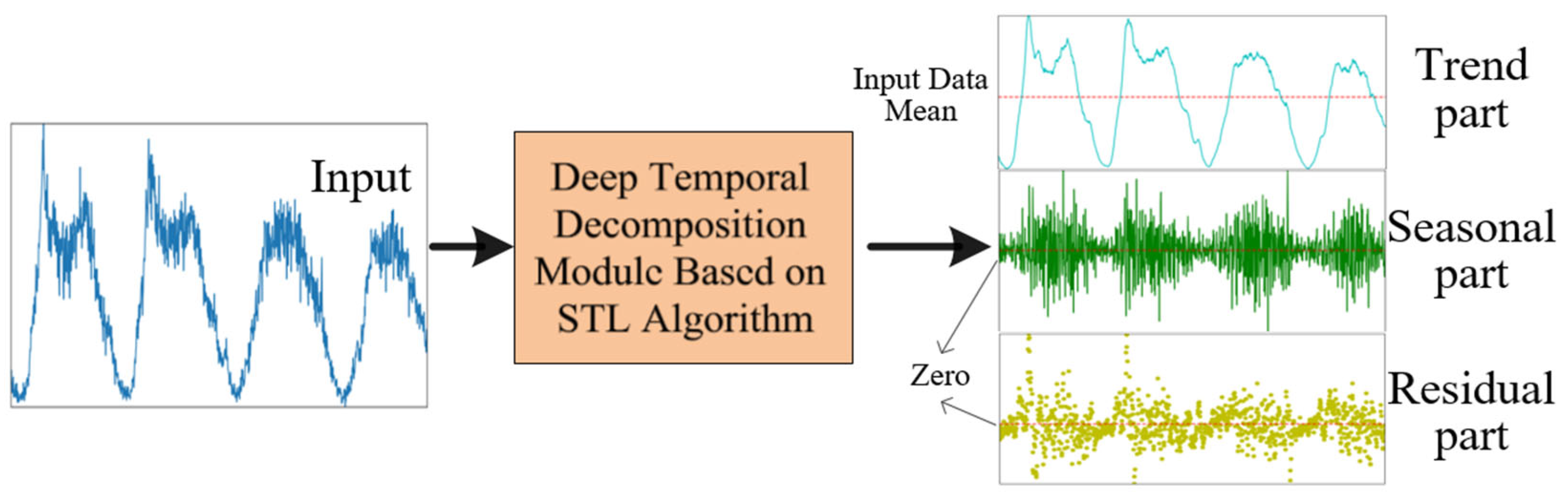
Based on the STL theory, we design a decomposition mechanism suitable for traffic flow time series. As shown in Figure 2, the input traffic sequence is decomposed into three parts: Trend, Seasonal, and Residual. The Trend component captures the gradual increasing or decreasing tendency of traffic flow, typically used to model long-term variations such as growth or decline in transportation demand. The Seasonal component represents seasonal fluctuations in the time series, usually short-term cyclical variations with regular patterns. In traffic flow forecasting, this component reflects recurrent patterns like peak/off-peak periods during a day or weekday/weekend differences. The Residual component captures unpredictable variations in the time series, typically representing random noise that cannot be explained by trend or seasonality. In traffic flow prediction, these residuals often correspond to abrupt changes caused by unexpected events such as traffic accidents or weather changes. Notably, while the residual component may be less influential in long-term forecasting where periodic patterns dominate, it plays a crucial role in capturing short-term, anomalous fluctuations, thereby enhancing the model’s robustness [23].

Figure 2. Schematic diagram of the deep temporal decomposition module based on STL algorithm.

The STL temporal decomposition processes the input sequence using the Locally Weighted Regression (Loess) method. Specifically, the seasonal component is obtained by applying padding and average pooling (AvgPool2d) operations to the input sequence, while the trend and residual components are derived through similar procedures as formulated in Equations (1)–(4):

$${\mathcal{X}}_t=T_t+S_t+R_t$$

(1)

$$S_t=AvgPool2d\left(Padding{(\mathcal{X}}_t\right))$$

(2)

$$T_t=AvgPool2d({Padding(\mathcal{X}}_t-S_t))$$

(3)

$$R_t={\mathcal{X}}_t-S_t-T_t$$

(4)

The padding operation ensures effective computation at sequence boundaries while preserving edge information, with the AvgPool2d layer serving as a locally weighted operator to reduce time complexity. This approach not only retains spatiotemporal characteristics of the data but also accelerates computation. The decomposition method effectively captures variation patterns in traffic flow sequences, thereby providing more refined temporal correlation information for subsequent prediction modeling. The seasonality window size in STL is set based on the fundamental periodicity of traffic flow (e.g., 288 time steps for a daily cycle with 5-min intervals), leveraging domain knowledge to ensure meaningful decomposition without introducing additional hyperparameters that require extensive tuning.

2.2. Autocorrelation and Delayed Aggregation

The proposed autocorrelation mechanism builds upon the theoretical foundation of self-attention [34], specifically designed to capture seasonal patterns in sequential data. Given the prominent cyclical variations inherent in traffic flow data, this seasonal modeling approach enables more accurate identification of fluctuation patterns, thereby improving prediction accuracy. Unlike Autoformer, which computes auto-correlation on a mixed representation of the decomposed series, our mechanism operates exclusively on the purified seasonal component, effectively filtering out interference from trend and noise. This seasonal-driven approach directly addresses challenge C2 by providing a more focused mechanism for capturing cyclical patterns. The autocorrelation mechanism establishes position-wise dependencies by leveraging seasonal information within the input sequence, facilitating sequence-to-sequence modeling. Unlike conventional attention mechanisms, it directly captures seasonal characteristics in time series through cyclical modeling, eliminating the need for explicit attention matrix construction. Consequently, this mechanism achieves reduced computational complexity while maintaining superior performance in long-sequence processing.

The autocorrelation mechanism operates through two sequential phases: (1) seasonal-dependent pattern discovery and (2) time-delay-based aggregation.

In the first phase, the mechanism identifies seasonal patterns in the input sequence by examining feature similarity between current traffic flow and historical time steps. Higher autocorrelation coefficients indicate stronger seasonal dependencies at corresponding temporal positions. The model determines the period length (i.e., traffic flow recurrence interval) through peak detection in the autocorrelation function. For seasonal signals, the autocorrelation function exhibits seasonal peaks, whereas for non-seasonal signals, it displays a decaying waveform without distinct peaks. Leveraging this seasonal-dependent principle, the model computes the autocorrelation matrix via Fourier transform to identify seasonal patterns. Specifically, for the input sequences ${\mathrm{Q}}_{\mathrm{t}}=\left({\mathrm{q}}_{\mathrm{t}+1},{\mathrm{q}}_{\mathrm{t}+2},\dots {\mathrm{q}}_{\mathrm{t}+\tau }\right)\in {\mathrm{R}}^{\tau \times \mathrm{N}\times \mathrm{F}}$, ${\mathrm{K}}_{\mathrm{t}}=\left({\mathrm{k}}_{\mathrm{t}+1},{\mathrm{k}}_{\mathrm{t}+2},\dots {\mathrm{k}}_{\mathrm{t}+\tau }\right)\in {\mathrm{R}}^{\tau \times \mathrm{N}\times \mathrm{F}}$ and ${\mathrm{V}}_{\mathrm{t}}=\left({\mathrm{v}}_{\mathrm{t}+1},{\mathrm{v}}_{\mathrm{t}+2},\dots {\mathrm{v}}_{\mathrm{t}+\tau }\right)\in {\mathrm{R}}^{\tau \times \mathrm{N}\times \mathrm{F}}$, the mathematical formulations are defined as follows:

$$Corr\left({\mathrm{Q}}_{\mathrm{t}}{,\mathrm{K}}_{\mathrm{t}}\right)={\mathcal{F}}^{-1}\left(\mathcal{F}\left({\mathrm{Q}}_{\mathrm{t}}\right){\mathcal{F}}^{*}\left({\mathrm{K}}_{\mathrm{t}}\right)\right)$$

(5)

$$\mathrm{C}\mathrm{o}\mathrm{r}\mathrm{r}\mathrm{e}\mathrm{l}\mathrm{a}\mathrm{t}\mathrm{i}\mathrm{o}\mathrm{n}\left({\mathrm{Q}}_{\mathrm{t}}{,\mathrm{K}}_{\mathrm{t}}{,\mathrm{V}}_{\mathrm{t}}\right)=Agg({\mathrm{V}}_{\mathrm{t}},Corr\left({\mathrm{Q}}_{\mathrm{t}}{,\mathrm{K}}_{\mathrm{t}}\right))$$

(6)

where $\mathcal{F}\left(·\right)$ and ${\mathcal{F}}^{-1}\left(·\right)$ denote the Fast Fourier Transform (FFT) and its inverse, respectively, and ${\mathcal{F}}^{*}\left(·\right)$ denotes the complex conjugate. This formulation enables efficient computation of sequence correlations in the frequency domain.

In the second phase, the model aggregates seasonal information by integrating multiple time-delayed versions of the signal to achieve more accurate and reliable results. This method is based on the core hypothesis that when temporally shifted versions of a signal exhibit similar features, their weighted aggregation through time delays can yield enhanced precision. The specific implementation involves generating multiple time-delayed signal versions to capture seasonal fluctuations:

$$k=⌊c\times log\tau ⌋$$

(7)

$${\tau }_1,{\tau }_2,\dots ,{\tau }_k=\underset{i\in \left\{1,2,\dots ,\tau \right\}}{\underbrace{\mathrm{a}\mathrm{r}\mathrm{g}Topk}}(Corr\left(Q_i{,K}_i\right))$$

(8)

where ⌊∙⌋ denotes the floor operation, c is the delay factor, $\tau$ is the sequence length, and the Top-k strategy (Equation (9)) is used to select the top k positions with the highest correlation for generating signal versions with different time delays. Measure signal similarity using an autocorrelation matrix to identify key seasonal points, perform weighted aggregation based on similarity to enhance seasonal features, and employ a sliding window technique to dynamically integrate information from different time windows while suppressing noise interference. This process effectively strengthens the model’s capability to model seasonal patterns; Using the Roll operation to delay and shift the signal, the final prediction information is obtained through aggregation:

$$Agg(V,Corr(Q,K))=\sum _{i=1}^{k}Roll\left(V,{\tau }_i\right)SoftMax\left(Corr\right(Q_{{\tau }_i}{,K}_{{\tau }_i}\left)\right)$$

(9)

where $Roll\left(V,{\tau }_i\right)$ denotes delaying the signal, Softmax is applied to normalize the correlation weights, and Agg represents the aggregation operation.

Through this time-delayed aggregation process, the model can learn the most relevant seasonal information from multiple time points relative to the current moment, thereby enhancing its predictive capability. In traffic flow prediction tasks, especially when dealing with noisy data, this method effectively extracts useful seasonal information, improving prediction stability and accuracy.

The autocorrelation mechanism combines seasonal information with time-delayed information, enabling the model to better understand seasonal and lagged relationships in time series data, which enhances prediction performance. Furthermore, the introduction of time-delayed aggregation allows the model to integrate information across multiple time scales, making it particularly suitable for traffic flow data with strong seasonal fluctuations.

To address the limitations of single-head autocorrelation mechanisms in modeling long sequences, this paper proposes a multi-head autocorrelation mechanism. The mechanism divides the input sequence into multiple subsequences, with each subsequence assigned an independent autocorrelation head that focuses on seasonal patterns at different time scales. The autocorrelation results from all heads are then aggregated to form the final global autocorrelation features. This approach effectively captures characteristics across diverse seasonal patterns, thereby enhancing the model’s capability to represent multi-scale seasonal variations.

By incorporating the multi-head autocorrelation mechanism, STLLformer demonstrates superior adaptability in multi-scale seasonal modeling. Particularly when processing traffic flow data with complex seasonal fluctuations, it significantly improves the model’s prediction accuracy and stability.

2.3. Graph-Based Spatial Modeling

To address the impact of spatial heterogeneity in traffic flow, and specifically to overcome the limitation of standard GCNs in capturing long-range dependencies (C3), this paper introduces a Low-rank Graph Convolutional Network (LGCN) for spatial information modeling and extraction. The LGCN decomposes the topological structure of traffic networks using the Lanczos algorithm and extracts low-rank dynamic factors of traffic flow through its Low-rank Dynamic Graph Filter (LDGF) module, thereby better establishing spatial dependencies between nodes. Unlike traditional graph convolution methods, the LGCN can effectively handle complex spatial relationships in large-scale traffic networks and achieve long-range spatial information interaction across nodes through multi-layer graph convolutions [35,36].

In the STLLformer model, the input sequence, ${\mathcal{X}}_{\mathrm{t}}\in {\mathrm{R}}^{\tau \times \mathrm{N}\times \mathrm{F}}$ is processed by the graph convolutional network to output spatial features:

$$T_t,{ S}_t, R_t=\mathrm{S}\mathrm{T}\mathrm{L}\mathrm{D}\mathrm{e}\mathrm{c}\mathrm{o}\mathrm{m}\mathrm{p}\left({\mathcal{X}}_{\mathrm{t}}\right)$$

(10)

Subsequently, the model further extracts spatial features through the LGCN and processes the seasonal components by integrating the multi-head autocorrelation mechanism:

$$\widehat{S_t}=\mathrm{L}\mathrm{G}\mathrm{C}\mathrm{N}(S_t+\mathrm{M}\mathrm{u}\mathrm{l}\mathrm{t}\mathrm{i}\mathrm{H}\mathrm{e}\mathrm{a}\mathrm{d}\left(S_t{W}_q,S_t{W}_k,S_t{W}_v\right)W_{\theta })$$

(11)

where $W_q,W_k,W_v,W_{\theta }$ are learnable weight matrices that enable the model to capture essential spatiotemporal features from the input traffic flow sequence. Subsequently, the model further extracts spatiotemporal features of traffic flow through low-rank decomposition:

$$\dot{T_t}, \dot{S_t}, \dot{R_t}=\mathrm{S}\mathrm{T}\mathrm{L}\mathrm{D}\mathrm{e}\mathrm{c}\mathrm{o}\mathrm{m}\mathrm{p}\left(\widehat{S_t}\right)$$

(12)

Finally, the encoder’s output combines the results from spatiotemporal convolution and low-rank graph convolution modules. This output serves as the decoder’s input (with seasonal components transmitted via cross-attention). The decoder separately models the trend, seasonal and residual components while integrating spatiotemporal features to generate final predictions:

$$Y_{t }=\left(\mathrm{L}\mathrm{G}\mathrm{C}\mathrm{N}\left(\dot{T_t}+T_t\right)\right)W_{trend }+(\dot{R_t}+R_t)W_{res}+\dot{S_t}{W}_{sea}$$

(13)

where W_trend, W_sea, W_res are learnable parameters for weighting the trend, seasonal and residual predictions, respectively. This weighted aggregation scheme allows the model to adaptively emphasize the most relevant components for different prediction horizons—with seasonal and trend components dominating long-term forecasts, while the residual component provides crucial adjustments for short-term anomalies.

The architecture captures spatial dependencies through the LGCN module, particularly effective for traffic flow prediction with complex spatial structures and seasonal variations. By combining low-rank graph convolution with seasonal modeling, STLLformer effectively extracts key spatial features and temporal patterns, significantly improving long-term traffic flow prediction accuracy and stability.

2.4. Encoder–Decoder Modeling

The STLLformer model adopts a standard encoder–decoder architecture and further enhances its spatiotemporal modeling capabilities through the synergistic interaction of the auto-correlation mechanism and graph convolution modules. In this structure, the input periodic component undergoes periodic modeling via the auto-correlation mechanism to generate periodic features, which are then processed by a graph convolutional network to extract spatial dependency features before being passed to the decoder.

In the decoder section, the trend component, periodic component, and residual component are modeled independently, and the information output by the encoder is integrated into the decoder through a cross-attention mechanism. Finally, the outputs of the three subsequences are weighted and combined to form the predicted future traffic flow. This component-specific modeling approach directly addresses challenge C1 by enabling specialized processing for each distinct temporal pattern in traffic flow.

This encoder–decoder framework effectively integrates temporal information with spatial structural information, strengthening the model’s ability to perceive complex traffic flow data. As a result, the model can simultaneously capture long-term trend variations, short-term periodic fluctuations, and sudden disturbances, making it adaptable to traffic flow prediction tasks across different time scales.

2.5. Datasets and Preprocessing

We conducted experiments by combining the public dataset PEMSD8 with the real self-built dataset HHY. The HHY dataset is derived from traffic data of a highway network in Zhejiang, China, comprising information from 490 ETC gantries across 276 road sections of 16 expressways. Each expressway consists of multiple road sections uniquely identified by start and end numbering, with each section containing 1–3 gantries. The attributes and recorded information of the gantry are shown in Table 2. The attributes of the gantry include gantry ID, relevant road segment information, mileage markers, and speed limits, which can be used to construct road network topology. The gantry records vehicle traffic data, including passing timestamps and vehicle IDs (OBUSN), providing a basis for calculating traffic flow and spatial average speed indicators. The dataset covers the period from 1 August 2020 to 30 November 2020. By analyzing the topological relationships among the original 490 gantries, we constructed an undirected graph network model, ultimately forming a research dataset containing 229 undirected nodes.

Table 2. Gantry attributes.

Start Segment ID	End Segment ID	Gantry ID	Start Milepost (km)	End Milepost (km)	Gantry Milepost (km)	Speed Limit (km/h)	Passage Time	OBUSN
1011	1013	G633110010	76.100	76.500	73.970	120	1 August 2020 12:26:37	00961108B421E1
1011	1013	G633110020	76.100	76.500	75.120	120	1 August 2020 12:28:06	00961108B421E1
1014	2701	G633210010	76.500	82.426	77.470	120	2 August 2020 16:07:32	10810012A115C7
1014	2701	G633210020	76.500	82.426	79.000	120	2 August 2020 18:57:16	70960008B28114
1014	2701	G633210030	76.500	82.426	81.000	120	7 August 2020 10:56:19	50960008B420D6
4017	4015	S933420010	71.495	64.060	66.528	100	10 August 2020 18:32:05	44010162009410
2901	2919	G133520020	1.7	0.53	1.12	80	11 August 2020 09:09:12	30962008B2815B

PEMSD8 is a publicly available traffic flow dataset provided by the California Department of Transportation’s (Caltrans) Performance Measurement System (PeMS), primarily used for traffic flow prediction and spatiotemporal data modeling research. The dataset is collected from California’s District 8 traffic management area, comprising recorded data from a total of 170 sensor nodes. The temporal coverage spans from 1 July 2016 to 31 August 2016.

3. Results

3.1. Benchmark Methods and Experimental Setup

This paper conducts comparative experiments between the STLLformer algorithm and four benchmark methods: (1) Historical Average (HA) [37]; (2) Auto-Regressive Integrated Moving Average (ARIMA) [6]; (3) Long Short-Term Memory networks (LSTM) [10]; and (4) Low-Rank Graph Convolutional Network (LSTGCN) [28].

All datasets adopt a 5-min interval, generating 288 daily samples, with training/validation/test sets split at a 6:2:2 ratio. A 6-h historical window (72 timesteps) was used to predict the subsequent 6-h flows (72 timesteps).

The model was trained using the Mean Squared Error (MSE) loss function, which penalizes larger errors more heavily and facilitates stable gradient-based optimization. For comprehensive evaluation, we employed three complementary metrics: Mean Absolute Error (MAE), Root Mean Squared Error (RMSE), and Mean Absolute Percentage Error (MAPE). MAE provides a robust measure of average error magnitude, RMSE emphasizes the impact of larger errors due to its squaring operation, and MAPE offers a scale-independent relative error perspective, which is particularly useful for comparing performance across different datasets or traffic conditions with varying flow volumes [38].

To ensure robust and statistically significant comparisons, all models for the 6-h prediction task on the HHY dataset were trained and evaluated over 10 independent runs with different random seeds. We report the mean ± standard deviation for these configurations in Table 2. Furthermore, paired t-tests were conducted between STLLformer and the strongest baseline (LSTGCN), confirming the significance of performance improvements (p < 0.01).

3.2. Sensitivity Analysis

The predictive performance of temporal deep learning models is highly dependent on the selection and configuration of hyperparameters. To systematically investigate the model’s internal influencing factors, we designed a comprehensive sensitivity analysis for the STLLformer model, focusing on two critical aspects: (1) Input feature analysis: comparing single-input (traffic flow only) versus multi-input configurations (incorporating traffic flow, speed, and occupancy) and (2) Multi-head attention mechanism: evaluating different head configurations (2-head, 4-head, and 6-head variants).

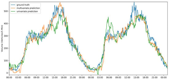
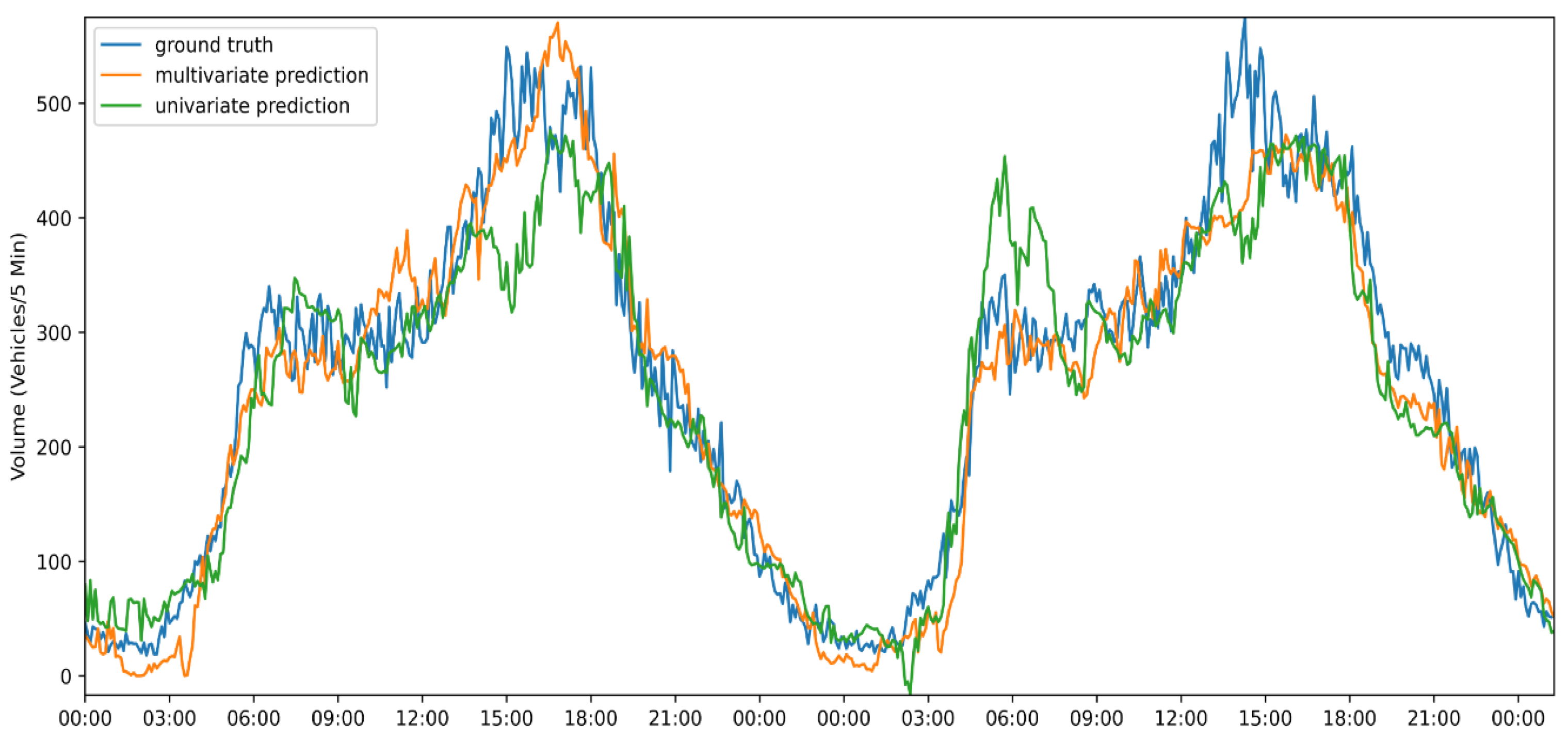
Our comparative experiments on the PEMSD8 dataset evaluated both single-feature (traffic flow only) and multi-feature (traffic flow, speed, and occupancy) input configurations. Using a 6-h historical window (72 timesteps) to predict the next 6-h period, Figure 3 shows the results for the 72nd prediction timestep from 23–24 February 2018. The results revealed that while both input types produced fundamentally consistent prediction trends, the multi-variable input demonstrated approximately 3% better accuracy during periods of significant fluctuation, particularly the bimodal peaks. This improvement confirms that incorporating multiple traffic parameters provides more comprehensive information, enabling predictions that more closely approximate actual observed values.

Figure 3. Prediction comparison for Node 26 in PEMSD8 dataset over a 48-h period.

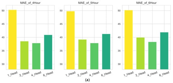
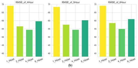
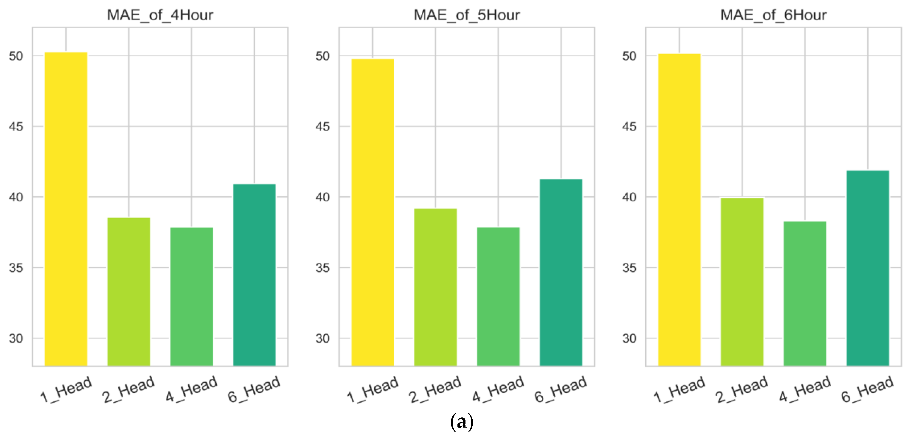
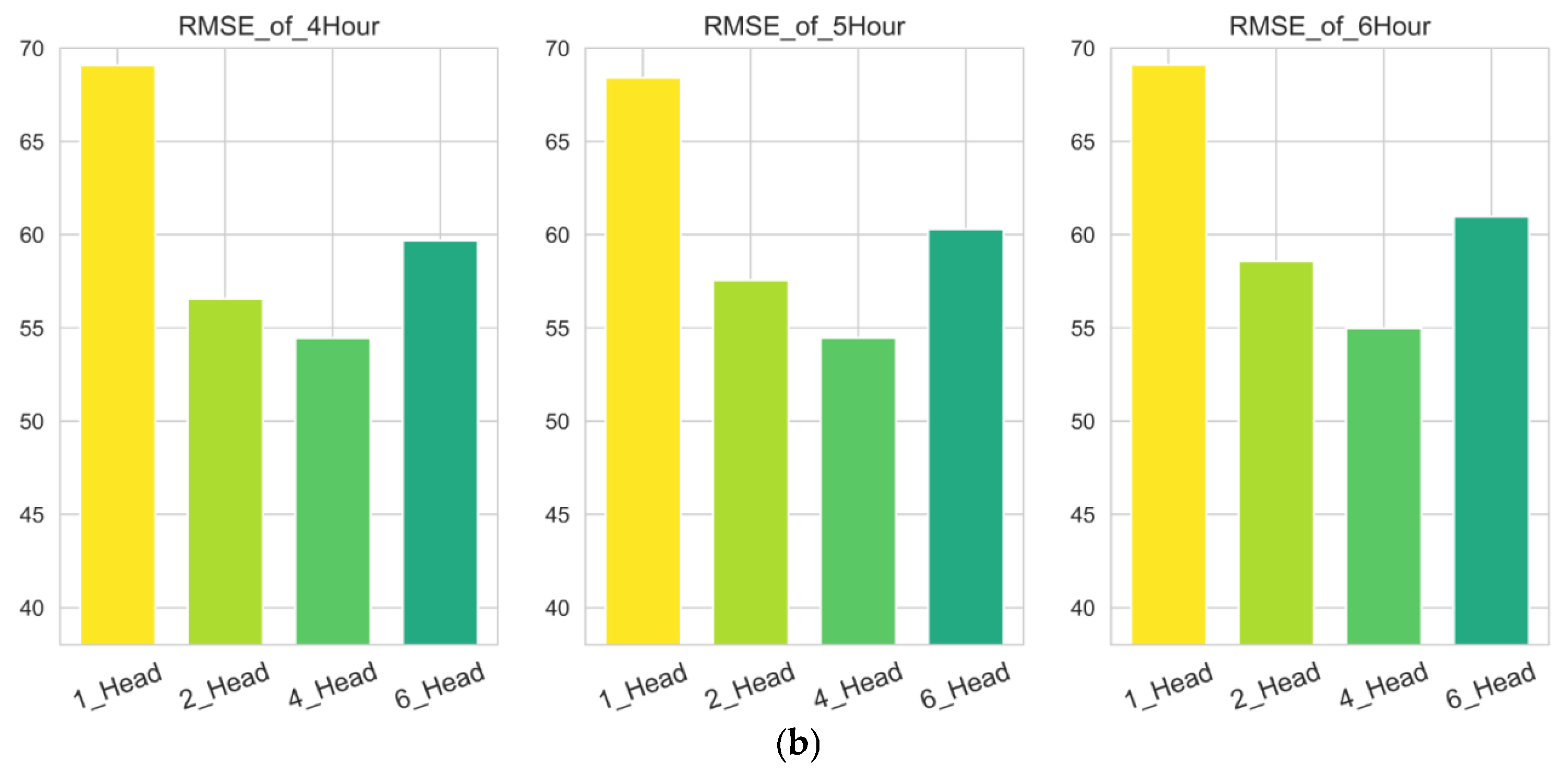
As shown in Figure 4, this paper compares the performance of multi-head attention mechanisms with different numbers of attention heads across various prediction horizons (4, 5, and 6 h) on the PEMSD8 dataset. The results demonstrate that the multi-head attention mechanism outperforms single-head attention across all prediction horizons, with average reductions in MAE and RMSE ranging from 5% to 25%. However, as the number of attention heads further increases (e.g., to 6 heads), slight fluctuations emerge in some prediction metrics, suggesting that excessive heads may introduce redundant computation and overfitting risks. Under the experimental conditions of this study, the 4-head configuration achieves the best performance across all metrics, balancing prediction accuracy and model stability.

Figure 4. Comparison of multi-head attention mechanisms with different numbers of heads on PMSD8, including (a) MAE under different prediction steps; (b) MAE under different prediction steps.

In summary, the sensitivity analysis confirms that a multi-variable input configuration and a 4-head attention mechanism are optimal choices for STLLformer, contributing to its stable and accurate performance.

3.3. Comparative Experiments

On both the HHY and PEMSD8 datasets, this study compared the performance of different long-term prediction methods across various prediction steps (48, 60, and 72 steps). Evaluation metrics included MAE, RMSE, and MAPE, with all results based on the average of 10 independent training runs (see Table 2).

As shown in Table 3, STLLformer outperformed all baseline models in the 6-h prediction task, with its MAE being approximately 20% lower on average than that of the second-best model, LSTGCN. This demonstrates its superiority in long-term traffic flow modeling. The improvements are statistically significant (p < 0.01 in paired t-tests against LSTGCN). Furthermore, the MAE reduction from 38.82 (±1.98) of LSTGCN to 30.67 (±1.11) of STLLformer on HHY for 6-h prediction translates to over 20% error reduction. In practical terms, this level of improvement in long-term forecasting accuracy can significantly enhance the reliability of traffic management systems for proactive congestion control and dynamic route guidance.

Table 3. Prediction Results of the Model on HHY and PEMSD8 Datasets.

Pred Length	Model	Dataset	HHY			PEMSD8
		Metrics	MAE	MAPE (%)	RMSE	MAE	MAPE (%)	RMSE
4 h	HA		75.912	93.772	96.957	99.5735	112.856	122.407
	ARIMA		63.710	78.212	83.283	83.325	94.341	107.824
	LSTM		52.998	73.442	76.487	72.094	86.245	96.522
	LSTGCN		33.235	47.653	51.376	36.868	45.726	54.456
	STLLformer		28.235	37.653	42.376	30.337	38.746	43.104
5 h	HA		73.194	89.073	93.528	103.308	119.064	126.622
	ARIMA		60.766	73.196	79.385	88.464	103.232	113.205
	LSTM		49.949	70.241	73.144	67.860	82.284	93.077
	LSTGCN		36.235	50.653	58.376	39.126	47.045	56.478
	STLLformer		29.349	38.381	43.588	31.960	39.032	43.537
6 h	HA		70.951	87.564	92.472	106.73	123.01	130.65
	ARIMA		59.595	71.621	76.072	92.766	105.35	117.537
	LSTM		47.480	68.521	70.201	64.544	80.623	89.467
	LSTGCN		38.818 ± 1.98	47.721 ± 3.11	53.909 ± 2.92	41.317	49.362	57.993
	STLLformer		30.665 ± 1.11	38.954 ± 1.96	44.033 ± 1.54	32.692	41.326	44.279

Among the compared models, traditional statistical methods (HA, ARIMA) performed the worst, particularly in long-term prediction tasks, where their errors were significantly higher than those of deep learning models. The reason lies in the fact that statistical models primarily focus on trend modeling in sequences, making them less capable of handling sudden fluctuations and nonlinear variations in traffic flow data.

The LSTM model, due to its reliance on unidirectional dependency modeling in time series, tends to forget early-stage information under long-term input scenarios, resulting in noticeably inferior prediction performance compared to LSTGCN and STLLformer, which incorporate graph convolution modules in their architectures. LSTGCN enhances the modeling of correlations between nodes by leveraging spatial adjacency information, further improving prediction accuracy.

Building upon LSTGCN, STLLformer introduces three key mechanisms: (1) The STL decomposition algorithm is employed to deconstruct the original time series into three sub-sequences—trend, seasonal, and residual—enabling separate modeling of different temporal dynamics. (2) A seasonal-dominated autocorrelation mechanism combined with a time-delay aggregation structure dynamically selects the most relevant historical nodes for the current time step, improving the accuracy and stability of seasonal fluctuation modeling. (3) A low-rank graph convolution module is designed to preserve low-rank features of the graph structure while enhancing interaction capabilities between spatially distant nodes. These mechanisms work synergistically, allowing STLLformer to achieve superior and more stable prediction results in long-term forecasting tasks on both datasets.

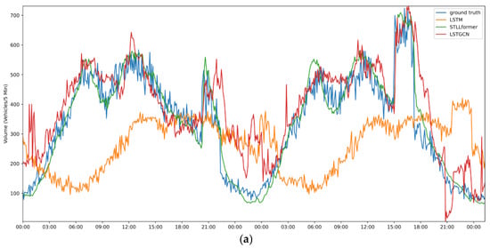
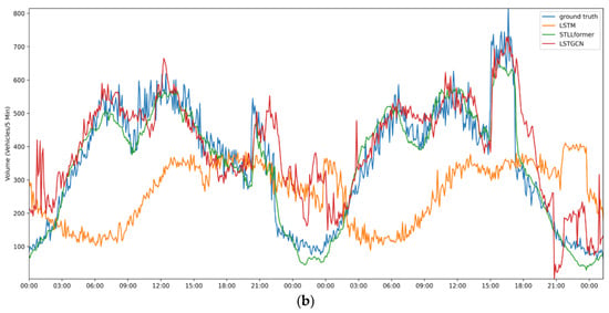
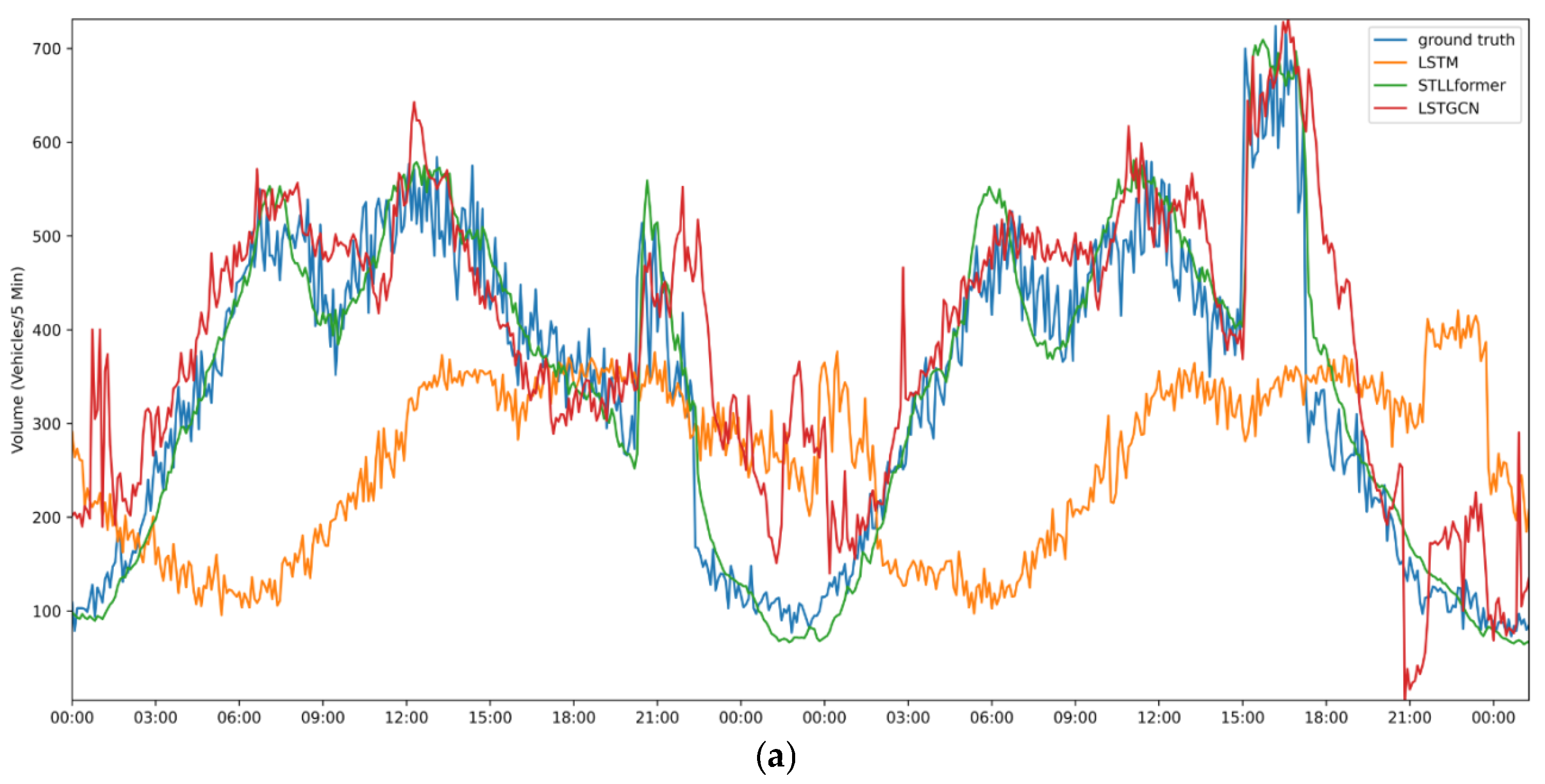
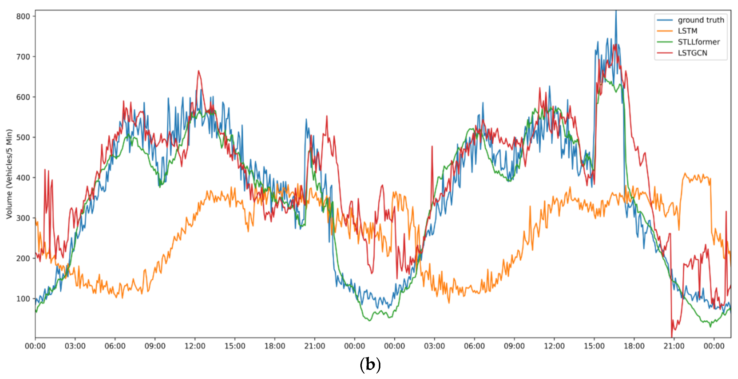
Figure 5 presents a comparison of the LSTM, LSTGCN, and STLLformer models at the 15th and 113th nodes of the HHY dataset. Compared to LSTGCN, STLLformer demonstrates superior performance in prediction accuracy and flow trend fitting. Particularly during periods of high fluctuation, STLLformer captures the true traffic flow patterns more effectively, highlighting its advantage in long-term forecasting.

Figure 5. Comparative prediction results of different models on the HHY dataset, including (a) Prediction results comparison at Node 15; (b) Prediction results comparison at Node 113.

Temporal Error Distribution and Model Stability

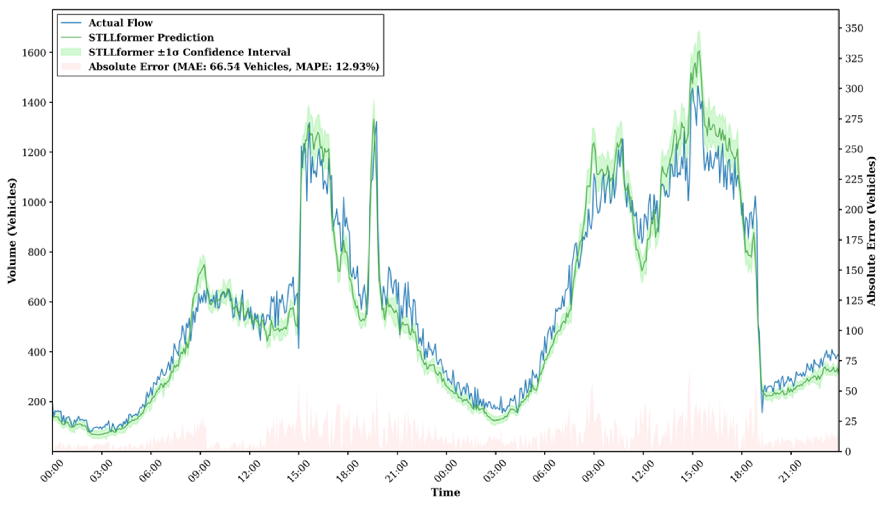
To assess model performance under realistic and operationally critical conditions, we selected a representative node known for handling high traffic volumes for a fine-grained temporal analysis. Figure 6 presents the comprehensive 48-h forecast for this node, integrating the ground truth, STLLformer predictions with ±1σ confidence intervals, and the instantaneous prediction errors. The model successfully captures the complex diurnal pattern of this high-flow location, with the prediction curve closely adhering to the ground truth and a narrow confidence band indicating stable performance across runs.

Figure 6. Traffic prediction with error magnitude visualization. Shows actual flow (blue), predicted flow (green) with confidence interval, and absolute error magnitude (pink) over a 48-h period. The height of the pink area corresponds to the prediction error at each time step.

The quantitative analysis of this high-volume scenario reveals an overall MAE of 66.54 vehicles, which corresponds to a MAPE of 12.93%. This level of relative error is commendable given the node’s elevated traffic volume and inherent volatility. A critical observation is the non-uniform distribution of error: the MAE during peak hours (102.52 vehicles) is 77.8% higher than during off-peak periods (57.66 vehicles). This disparity, however, is contextualized by the fact that peak traffic volume at this node is approximately 2.5 times greater than off-peak volume. Consequently, the model’s relative accuracy (MAPE) remains robust across both conditions. The elevated absolute error during peaks is therefore not an indicator of model failure, but rather a reflection of the increased forecasting difficulty associated with high-density, stop-and-go traffic dynamics. This performance profile underscores the model’s practical utility, as it delivers reliable and interpretable forecasts under the most demanding and consequential traffic states, where accurate forecasting is paramount for effective management.

3.4. Ablation Study

To further investigate the effects of different modules in STLLformer, this paper designs three variants of the STLLformer model and compares them on the PEMSD8 dataset. All models share the same number of Encoder and Decoder layers, with the attention mechanism’s d_model set to 64, the number of multi-head attention heads set to 4, and M in the low-rank graph convolutional layer set to 100. The differences between the models are shown in Table 4.

Table 4. Model Architecture Comparison.

Model Name	Structural Description
SeriseSTModel	Decomposition mechanism (trend + seasonal) + encoder–decoder
SeriseLSTModel	Decomposition mechanism (trend + seasonal) + LGCN + encoder–decoder
STLLformer1	STL (trend + seasonal + residual) + seasonal-driven autocorrelation + LGCN + encoder–decoder
STLLformer	STL (trend + seasonal + residual) seasonal-driven autocorrelation + LGCN + encoder–decoder + enhances long-transfer

Table 5 shows the long-term forecasting performance of three STLLformer variants on the PEMSD8 dataset. The experimental results indicate:

Table 5. Forecasting Results of Ablation Models on the PEMSD8 Dataset.

Pred Length	Model	Dataset	HHY
		Metrics	MAE	MAPE (%)	RMSE
4 h	SeriseSTModel		73.033	78.761	89.136
	SeriseLSTModel		45.111	57.442	64.011
	STLLformer1		40.843	49.956	58.271
	STLLformer		30.337	38.746	43.104
5 h	SeriseSTModel		73.485	79.903	89.601
	SeriseLSTModel		45.495	59.012	64.520
	STLLformer1		41.296	50.264	59.077
	STLLformer		31.96	39.032	43.537
6 h	SeriseSTModel		75.705	80.542	102.703
	SeriseLSTModel		46.318	46.213	65.237
	STLLformer1		41.893	42.643	59.797
	STLLformer		32.692	41.326	44.279

Models incorporating the LGCN module (i.e., adding spatial feature modeling based on SeriesSTModel) reduced long-term prediction errors by approximately 39% to 61% compared to models without LGCN, validating the effectiveness of the LGCN module in capturing spatial dependency features of traffic flow sequences. The STLLformer series models (integrating STL decomposition algorithm) further reduced prediction errors by 8% to 18% compared to other models, demonstrating that structurally decomposing sequences into trend, seasonal, and residual components helps develop more targeted feature extraction strategies, thereby improving overall forecasting performance. When comparing STLLformer1 (using the trend component as the main subsequence) with STLLformer2 (using the seasonal component as the main subsequence), it was found that the seasonal-driven autocorrelation mechanism performed better in long-term forecasting tasks, with error reductions reaching 26% to 30%. The results show that the seasonal component plays a key role in capturing the repetitiveness and time-lagged characteristics of traffic flows.

In summary, the ablation study validates the individual and combined contribution of each proposed module, with the STL decomposition and the seasonal-driven autocorrelation mechanism being the most significant contributors to the final performance.

3.5. Discussions

The experimental results presented in the previous sections establish STLLformer as a robust framework for long-term traffic forecasting. Beyond the quantitative metrics, our analysis yields deeper insights into the model’s operational characteristics and its practical implications.

A central finding of this work is the empirical validation of the multi-component modeling strategy. The superior performance of STLLformer can be largely attributed to its explicit handling of the distinct temporal patterns inherent in traffic flow. The seasonal component, processed by the dedicated autocorrelation mechanism, proves to be the dominant factor for long-term accuracy, effectively capturing the recurring peaks and troughs of daily and weekly cycles. This explains the model’s pronounced accuracy in forecasting the overall traffic rhythm, as visually confirmed in Figure 6. Conversely, while the residual component’s influence is less pronounced in long-horizon predictions, its role is crucial for capturing transient, non-periodic fluctuations. This delineation suggests that the residual component would become increasingly critical in short-term forecasting scenarios or when modeling the impact of unexpected events, offering a clear pathway for model adaptation.

From a practical standpoint, the observed performance profile—characterized by robust overall accuracy and reliable peak-period forecasting—holds significant value for traffic management systems. The model’s ability to provide stable, hours-ahead predictions enables a shift from reactive to proactive traffic control. For instance, accurate forecasts of impending peak-hour volumes can inform dynamic speed limit adjustments and pre-emptive congestion mitigation strategies, while reliable long-term trend predictions can optimize infrastructure maintenance scheduling. The fact that the model maintains reasonable relative error (MAPE) even during high-volume, high-variability peak hours underscores its operational reliability when it is needed most.

In conclusion, STLLformer introduces a principled approach to long-term traffic forecasting by structurally decomposing and modeling the heterogeneous nature of traffic flow. The framework not only achieves state-of-the-art performance but also provides a more interpretable and adaptable foundation for intelligent transportation systems, where understanding and forecasting complex temporal dynamics is key to enhancing efficiency and sustainability.

4. Conclusions

This paper has introduced STLLformer, a novel spatiotemporal Transformer framework that establishes a seasonal-dominated, multi-component collaborative paradigm for long-term traffic flow forecasting. The model’s core innovation lies in its dedicated architecture, which integrates STL decomposition to separately model trend, seasonal, and residual components, a seasonal-driven autocorrelation mechanism for purified temporal dependency capture, and a low-rank graph convolution module to effectively model long-range spatial dependencies.

Comprehensive experiments on two real-world highway datasets demonstrate that STLLformer significantly and consistently outperforms a range of state-of-the-art benchmarks. The performance improvement is statistically significant, as validated by multiple runs, and is practically meaningful. A key insight from our temporal analysis is that the model provides particularly reliable forecasts during operationally critical peak traffic hours, despite the increased volatility inherent to these periods.

Beyond achieving superior accuracy, this work provides a more interpretable and principled framework for traffic forecasting by explicitly acknowledging and modeling the heterogeneous nature of traffic flow. The decomposition-based approach not only enhances performance but also offers a clear pathway for model adaptation and improvement. Future work will focus on integrating real-time external events to improve robustness during anomalies and exploring the framework’s transferability to other spatiotemporal forecasting domains.

References

- Zhao, L.; Song, Y.; Zhang, C.; Liu, Y.; Wang, P.; Lin, T.; Deng, M.; Li, H. T-GCN: A temporal graph convolutional network for traffic prediction. IEEE Trans. Intell. Transp. Syst. 2020, 21, 3848–3858. [Google Scholar] [CrossRef] [Scilit]
- Cai, D.Q.; Chen, K.W.; Lin, Z.Z.; Li, D.; Zhou, T.; Leung, M.F. JointSTNet: Joint Pre-Training for Spatial-Temporal Traffic Forecasting. IEEE Trans. Consum. Electron. 2025, 71, 6239–6252. [Google Scholar] [CrossRef] [Scilit]
- Jiang, W.; Luo, J. Graph neural network for traffic forecasting: A Survey. Expert Syst. Appl. 2022, 207, 117921. [Google Scholar] [CrossRef] [Scilit]
- Du, S.; Yang, T.; Teng, F.; Zhang, J.; Li, T.; Yu, Z. Multi-scale feature enhanced spatio-temporal learning for traffic flow forecasting. Knowl.-Based Syst. 2024, 294, 111787. [Google Scholar] [CrossRef] [Scilit]
- Cui, Z.; Henrickson, K.; Ke, R.; Wang, Y. Traffic graph convolutional recurrent neural network: A deep learning framework for network-scale traffic learning and forecasting. IEEE Trans. Intell. Transp. Syst. 2020, 21, 4883–4894. [Google Scholar] [CrossRef] [Scilit]
- Zhou, H.; Zhang, S.H.; Peng, J.Q.; Zhang, S.; Li, J.X.; Xiong, H.; Zhang, W.C. Informer: Beyond efficient transformer for long sequence time-series forecasting. In Proceedings of the 35th AAAI Conference on Artificial Intelligence, Online, 2–9 February 2021. [Google Scholar] [CrossRef] [Scilit]
- Eren, Y.; Küçükdemiral, İ. A comprehensive review of deep learning approaches for short-term load forecasting. Renew. Sustain. Energy Rev. 2024, 189, 114031. [Google Scholar] [CrossRef] [Scilit]
- Jiang, R.H.; Wang, Z.N.; Yong, J.W.; Jeph, P.; Chen, Q.J.; Kobayashi, Y.; Song, X.; Fukushima, S.; Suzumura, T. Spatio-temporal meta-graph learning for traffic forecasting. In Proceedings of the 37th AAAI Conference on Artificial Intelligence, Washington, WA, USA, 7–14 February 2023. [Google Scholar]
- Lin, Y.L.; Dai, X.Y.; Li, L.; Wang, F.Y. Pattern sensitive prediction of traffic flow based on generative adversarial framework. IEEE Trans. Intell. Transp. Syst. 2019, 20, 2395–2400. [Google Scholar] [CrossRef] [Scilit]
- Shi, X.J.; Chen, Z.R.; Wang, H.; Yeung, D.Y.; Wong, W.K.; Woo, W.C. Convolutional LSTM network: A machine learning approach for precipitation nowcasting. In Proceedings of the 29th Annual Conference on Neural Information Processing Systems, Montreal, QC, Canada, 7–12 December 2015. [Google Scholar]
- Zhang, W.S.; Yao, R.H.; Yuan, Y.; Du, X.J.; Wang, L.B.; Sun, F. A traffic-weather generative adversarial network for traffic flow prediction for road networks under bad weather. Eng. Appl. Artif. Intell. 2024, 137, 109125. [Google Scholar] [CrossRef] [Scilit]
- Huang, B.Y.; Dou, H.W.; Luo, Y.; Li, J.C.; Wang, J.Q.; Zhou, T. Adaptive spatiotemporal transformer graph network for traffic flow forecasting by IoT loop detectors. IEEE Internet Things J. 2023, 10, 1642–1653. [Google Scholar] [CrossRef] [Scilit]
- Wu, Z.; Pan, S.; Chen, F.; Long, G.; Jiang, J.; Zhang, C.Q. Graph wavenet for deep spatial-temporal graph modeling. In Proceedings of the 28th International Joint Conference on Artificial Intelligence, Macao, China, 10–16 August 2019. [Google Scholar] [CrossRef] [Scilit]
- Li, Y.; Yu, R.; Shahabi, C.; Liu, Y. Diffusion convolutional recurrent neural network: Data-driven traffic forecasting. In Proceedings of the 6th International Conference on Learning Representations, Vancouver, BC, Canada, 30 April–3 May 2018. [Google Scholar]
- Yu, B.; Yin, H.; Zhu, Z. Spatio-temporal graph convolutional networks: A deep learning framework for traffic forecasting. In Proceedings of the 27th International Joint Conference on Artificial Intelligence, Stockholm, Sweden, 13–19 July 2018. [Google Scholar] [CrossRef] [Scilit]
- Guo, S.; Lin, Y.; Feng, N.; Song, C.; Wan, H. Attention based spatial-temporal graph convolutional networks for traffic flow forecasting. In Proceedings of the 33rd AAAI Conference on Artificial Intelligence, Honolulu, HI, USA, 27 January–1 February 2019. [Google Scholar] [CrossRef] [Scilit]
- Song, C.; Lin, Y.; Guo, S.; Wan, H. Spatial-temporal synchronous graph convolutional networks: A new framework for spatial-temporal network data forecasting. In Proceedings of the 34th AAAI Conference on Artificial Intelligence, New York, NY, USA, 7–12 February 2020. [Google Scholar] [CrossRef] [Scilit]
- Xu, Y.; Han, L.Z.; Zhu, T.Y.; Sun, L.L.; Du, B.W.; Lv, W.F. Generic dynamic graph convolutional network for traffic flow forecasting. Inf. Fusion 2023, 100, 101946. [Google Scholar] [CrossRef] [Scilit]
- Geng, W.; Pan, Y.; Xing, Z.; Liu, D.; Liu, R.; Zhu, Y. MSCMHMST: A traffic flow prediction model based on transformer. arXiv 2025. [Google Scholar] [CrossRef] [Scilit]
- Wang, X.; Ma, Y.; Wang, Y.; Jin, W.; Wang, X.; Tang, J.; Jia, C.; Yu, J. Traffic flow prediction via spatial temporal graph neural network. In Proceedings of the 29th World Wide Web Conference, Taipei, Taiwan, China, 20–24 April 2020. [Google Scholar] [CrossRef] [Scilit]
- Wu, H.X.; Xu, J.H.; Wang, J.M.; Long, M.S. Autoformer: Decomposition transformers with auto-correlation for long-term series forecasting. In Proceedings of the 35th Annual Conference on Neural Information Processing Systems, Online, 6–14 December 2021. [Google Scholar]
- Wu, Y.; Hou, M.; Hu, H. ACENet: Adaptive correlation-enhanced network for multivariate time series forecasting. Digit. Signal Prog. 2025, 167, 105424. [Google Scholar] [CrossRef] [Scilit]
- Wu, H.; Hu, T.; Liu, Y.; Zhou, H.; Wang, J.; Long, M. TimesNet: Temporal 2D-variation modeling for general time series analysis. arXiv 2022. [Google Scholar] [CrossRef] [Scilit]
- Seo, H.; Lim, C. ST-MTM: Masked time series modeling with seasonal-trend decomposition for time series forecasting. In Proceedings of the 31st ACM SIGKDD Conference on Knowledge Discovery and Data Mining, Toronto, ON, Canada, 3–7 August 2025. [Google Scholar]
- Zhu, C.; Chen, J.; Zhu, R.; Wang, Z.Q.; Liu, S.H.; Wang, J.S. ASTHGCN: Adaptive spatio-temporal hypergraph convolutional network for traffic forecasting. In Proceedings of the 30th IEEE International Conference on Software Analysis, Evolution and Reengineering, Macao, China, 21–24 March 2023. [Google Scholar] [CrossRef] [Scilit]
- Huang, H.; Lee, J.H.; Ge, Y.L.; Roh, S.B.; Zhao, X. Adaptive spatial–temporal graph attention network for real-time traffic forecasting. Eng. Appl. Artif. Intell. 2026, 163, 112883. [Google Scholar] [CrossRef] [Scilit]
- Jiang, J.; Han, C.; Zhao, W.X.; Wang, J. PDFormer: Propagation delay-aware dynamic long-range transformer for traffic flow forecasting. In Proceedings of the 37th AAAI Conference on Artificial Intelligence, Washington, WA, USA, 7–14 February 2023. [Google Scholar]
- Remmouche, B.; Boukraa, D.; Zakharova, A.; Bouwmans, T.; Taffar, M. Long-term spatio-temporal graph attention network for traffic forecasting. Expert Syst. Appl. 2025, 288, 128244. [Google Scholar] [CrossRef] [Scilit]
- Cleveland, R.B.; Cleveland, W.S.; McRae, J.E.; Terpenning, I. STL: A seasonal-trend decomposition procedure based on loess. J. Off. Stat. 1990, 6, 3–33. [Google Scholar]
- Jin, M.; Koh, H.Y.; Wen, Q.S.; Zambon, D.; Alippi, C.; Webb, G.I. A survey on graph neural networks for time series: Forecasting, classification, imputation, and anomaly detection. IEEE Trans. Pattern Anal. Mach. Intell. 2024, 46, 10466–10485. [Google Scholar] [CrossRef] [Scilit]
- Li, J.D.; Pan, W.; Deng, Q.P.; Wang, Z.; Zhu, W.W. STG-Meta: Spatial-temporal graph meta-learning for traffic forecasting. In Proceedings of the 2021 International Joint Conference on Neural Networks, Shenzhen, China, 18–22 July 2021. [Google Scholar]
- Li, M.; Zhu, Z. Spatial-temporal fusion graph neural networks for traffic flow forecasting. In Proceedings of the 35th AAAI Conference on Artificial Intelligence, Online, 2–9 February 2021. [Google Scholar]
- Chen, X.Q.; Ma, F.; Wu, Y.Z.; Han, B.; Luo, L.J.; Biancardo, S.A. MFMDepth: MetaFormer-based monocular metric depth estimation for distance measurement in ports. Comput. Ind. Eng. 2025, 207, 111325. [Google Scholar] [CrossRef] [Scilit]
- Li, S.; Jin, X.; Xuan, Y.; Zhou, X.; Chen, W.; Wang, Y.; Yan, X. Enhancing the locality and breaking the memory bottleneck of transformer on time series forecasting. In Proceedings of the 33rd Conference on Neural Information Processing Systems, Vancouver, BC, Canada, 8–14 December 2019. [Google Scholar]
- Gou, Z.; Shen, Y.G.; Chen, S.F. Lanczos method for spatio-temporal graph convolutional networks to forecast expressway flow. IET Intell. Transp. Syst. 2023, 17, 1979–1991. [Google Scholar] [CrossRef] [Scilit]
- Zhuang, Y.F.; Liu, P.; Yang, H.; Zhang, K.; Wang, Y.H.; Pu, Z.Y. Few-shot learning for novel object detection in autonomous driving. Commun. Transp. Res. 2025, 5, 100194. [Google Scholar] [CrossRef] [Scilit]
- Li, L.; Su, X.; Wang, Y.; Lin, Y.; Li, Z.; Li, Y. Robust causal dependence mining in big data network and its application to traffic flow predictions. Transp. Res. Part C–Emerg. Technol. 2015, 58, 292–307. [Google Scholar] [CrossRef] [Scilit]
- Chai, T.; Draxler, R.R. Root mean square error (RMSE) or mean absolute error (MAE)?—Arguments against avoiding RMSE in the literature. Geosci. Model Dev. 2014, 7, 1247–1250. [Google Scholar] [CrossRef] [Scilit]
Disclaimer/Publisher’s Note: The statements, opinions and data contained in all publications are solely those of the individual author(s) and contributor(s) and not of MDPI and/or the editor(s). MDPI and/or the editor(s) disclaim responsibility for any injury to people or property resulting from any ideas, methods, instructions or products referred to in the content. |
© 2025 by the authors. Licensee MDPI, Basel, Switzerland. This article is an open access article distributed under the terms and conditions of the Creative Commons Attribution (CC BY) license (https://creativecommons.org/licenses/by/4.0/).