Abstract
An in-depth and comprehensive evaluation of carbon emission efficiency (CEE) is essential for promoting high-quality development and achieving the “dual-carbon” goals. This study applies a super-efficiency slacks-based measure (Super-SBM) model with carbon emissions treated as an undesirable output to measure provincial CEE and the Malmquist–Luenberger (ML) index across 30 provinces and major comprehensive economic zones in China from 2010 to 2023. Efficiency trends for 2024–2025 are projected using a hybrid Autoregressive Integrated Moving Average (ARIMA)–Long Short-Term Memory (LSTM) approach. Furthermore, CEE patterns are examined at both national and regional levels, and the relationships between CEE and potential drivers are analyzed using Tobit regressions. Combining the regression outcomes with short-term forecasts, this study provides a forward-looking perspective on the evolution of CEE and its associated factors. The results indicate that (1) China’s CEE demonstrates a generally fluctuating upward trajectory, with the southern coastal and eastern coastal regions maintaining the highest efficiency levels, while other regions remain relatively lower. (2) The temporal changes in CEE across economic zones correspond to variations in technical efficiency and technological progress, with the latter contributing more prominently to overall improvement. (3) CEE shows significant associations with multiple factors: population density, economic development, technological advancement, government intervention, and environmental regulation are positively associated with efficiency, whereas urbanization tends to correlate negatively. Based on these findings, policy implications are discussed to promote differentiated pathways for enhancing CEE across China’s regions.
1. Introduction
Recent global uncertainties—arising from pandemics, geopolitical conflicts, and market disruptions—have heightened the urgency of improving carbon efficiency as a means to strengthen economic resilience [1]. Environmental challenges, particularly greenhouse gas emissions, will exert a substantial impact on human society and have become a foremost concern for nations worldwide. China is currently undergoing rapid urbanization and industrialization and is a major global consumer of energy and a significant emitter of carbon. In 2020, the government announced the goals of peaking carbon emissions within 10 years and achieving carbon neutrality within 40 years. These “dual-carbon” objectives, reaffirmed in the 2022 national strategy, emphasize low carbon economic transformation, green industry development, and sustainable lifestyles. Balancing economic growth and emission reduction has thus become a central challenge for China’s transition to high-quality development. Enhancing CEE provides a pathway to reduce emissions without constraining energy use, serving as a key measure to achieve sustainable growth [2,3].
Over the past decade, research on CEE has expanded along several major directions. First, measurement studies have employed DEA or SBM models to evaluate city and province level carbon-efficiency performance, revealing clear regional disparities. Second, dynamic decomposition studies have used the ML index to separate efficiency change (EC) and technological change (TC) effects. Third, driver identification analyses have applied Tobit or spatial econometric models to explore how factors relate to CEE. Fourth, forecasting studies have introduced ARIMA, LSTM, and hybrid models to predict trends in energy use and CEE. Despite these advances, several limitations remain: (1) Most studies focus on a single spatial scale, lacking integrated comparisons across provinces and economic regions. (2) The processes of efficiency measurement, factor analysis, and forecasting are usually conducted separately, without forming a coherent analytical chain. (3) Many studies adopt static frameworks, overlooking the dynamic evolution and future trajectories of CEE.
To address the gaps, this study develops an integrated and cross-scale analytical framework that connects historical evaluation with near-term forecasting. Firstly, it establishes a dual-scale comparison framework at the province–economic zone levels, identifying both inter-regional and intra-regional heterogeneity in CEE evolution. Secondly, it applies the Super-SBM model with undesirable outputs and the ML index to comprehensively measure static and dynamic efficiency. Thirdly, it employs a Tobit regression model to investigate the associations between efficiency and its main influencing factors and regional heterogeneity. Lastly, it introduces an ARIMA–LSTM hybrid model to forecast CEE trends for 2024–2025, linking historical assessments (2010–2023) with short-term outlooks. This unified framework integrates measurement, decomposition, influencing factors analysis, and forecasting within one empirical system. By bridging previously fragmented approaches, it offers a forward-looking understanding of China’s CEE evolution and provides actionable evidence for differentiated policy design across the eight comprehensive economic zones.
2. Literature Review
Carbon emission is a commonly used indicator for measuring the low carbon development level of a region and can essentially be regarded as a type of input-output efficiency [4]. Although various definitions of CEE have been proposed by scholars both domestically and internationally, no universally accepted standard exists. Broadly, definitions can be grouped into single-factor and multi-factor categories based on the factors considered during measurement.
Typical single-factor measures include carbon productivity [5], the carbon index [6,7], and carbon emissions intensity [8,9,10]. Other common single-factor indicators include per capita carbon emissions and energy intensity [11,12]. However, such indicators do not capture the interactions among multiple inputs and therefore cannot fully reflect production–emission relationships. To address this limitation, total-factor carbon-emission efficiency (TFCEE) has become the mainstream indicator. TFCEE is defined as the maximum economic output and minimum carbon emissions achievable without increasing capital, labor, or energy inputs, reflecting the degree of coordination between economic development and environmental constraints [13].
Two principal approaches are widely used to estimate TFCEE: the stochastic frontier approach (SFA) [14,15,16] and data envelopment analysis (DEA) [17,18,19,20]. Each has strengths and weaknesses—SFA relies on functional form assumptions, while DEA may overlook slacks and undesirable outputs. To improve these, SBM models [21] and DEA extensions that explicitly incorporate undesirable outputs [22] have been developed. The SBM model proposed by Tone is a non-radial, non-oriented variant of the conventional DEA framework. It evaluates efficiency by directly incorporating input and output slacks into the objective function, thereby overcoming the radial limitations of the traditional models. Andersen and Petersen’s Super-SBM model [23] extended this framework to the Super-SBM model, which distinguishing decision-making units (DMUs) operating on the frontier, thus improving discriminatory power. The Super-SBM model has been extensively applied in CEE research at different scales, including Central and Eastern European countries [4], Chinese cities [24,25,26], and sectoral contexts such as transportation [27,28], construction [29,30], and tourism [31,32]. Although the Super-SBM model has been widely applied in provincial level studies of CEE. For instance, A bibliometric synthesis is provided showing that DEA- and SBM-based efficiency models have become dominant methodological tools in carbon footprint and emission efficiency research, reflecting their transparency and comparability across regions [33], it remains a well-established and transparent framework for cross provincial comparison. Building upon this foundation, the present study adopts a Super-SBM with undesirable outputs to ensure consistent measurement and combines it with dynamic decomposition and forecasting to provide a more comprehensive evaluation. This approach enables the analysis to link static and dynamic efficiency, offering a unified perspective on CEE measurement and prediction.
In parallel, the spatial resolution of CEE research has advanced. Scholarship has progressed from macro-level analyses [3,34] to more granular investigations at provincial [1,3,35], city levels [36,37,38,39,40], and river-basin levels [41,42,43,44]. Nevertheless, most studies still rely on the traditional “East–Central–West” regional division, which fails to capture substantial differences in industrial structures, economic conditions, and resource endowments. To overcome this limitation, some researchers have adopted the “Eight Comprehensive Economic Zones” framework as a more policy relevant classification. Yet few studies have systematically analyzed CEE within this framework while simultaneously examining how alternative zoning and industrial structures shape efficiency disparities.
The evolution of CEE results from the interaction of multiple socioeconomic and policy factors. Accurately identifying these determinants is essential for developing targeted green development and emission reduction strategies. Empirical studies commonly employ the Spatial Durbin Model (SDM) [45,46,47], Geographically Weighted Regression (GWR) [48,49], and Tobit regression [50,51] to explore these relationships. However, most research focuses on static relationships or isolated variables, leaving an insufficient understanding of the time-varying and region-specific dynamics of CEE. In addition, the policy dimension of China’s carbon transition has begun to attract increasing academic attention. Researchers have highlighted how the nation’s carbon-neutrality commitment evolved from a strategic vision into a set of concrete policy actions [52], demonstrating that well-defined implementation pathways can enhance both market confidence and environmental performance. This policy-driven transition underscores the importance of integrating dynamic efficiency evaluation with actionable policy insights when examining China’s CEE.
Beyond conventional DEA and Tobit models, recent studies have advanced CEE research using metafrontier, spatial Durbin, and network DEA frameworks. Metafrontier analyses allow for heterogeneous regional technologies and show that most efficiency gaps stem from technological rather than managerial differences. Coastal provinces generally operate closer to the global frontier, while inland areas improve mainly through catch-up effects. Our pooled Super-SBM with undesirable outputs and ML decomposition produces comparable findings—technical change remains the dominant driver of national improvement, consistent with metafrontier evidence that progress largely reflects frontier expansion rather than internal efficiency gains.
Spatial Durbin and network DEA studies further reveal that CEE exhibits positive regional spillovers and that abatement sub-processes lag behind production efficiency. Our results are consistent with these patterns: regions with dense economic linkages and cleaner industrial structures achieve faster CEE growth, while energy-intensive areas progress more slowly. These comparisons confirm that the integrated Super-SBM and ML–Tobit framework used here aligns with the direction and scale of recent metafrontier, SDM, and network DEA findings while providing a unified, reproducible approach to dynamic regional CEE assessment.
To fill these gaps, this study conducts a comprehensive measurement and forecast of provincial CEE from both static and dynamic perspectives, while integrating factor analysis and cross regional comparisons. Specifically, it treats energy, capital, and labor as inputs; regional GDP as a desirable output; and carbon emissions as an undesirable output. Using the Super-SBM model (2010–2023) and a hybrid ARIMA–LSTM approach (forecasting 2024–2025), the paper examines the spatiotemporal evolution and determinants of CEE under the eight comprehensive economic zones framework. By linking measurement, decomposition, determinant analysis, and prediction within a unified empirical structure, this study bridges historical assessment and short-term forecasting, offering both theoretical insight and practical guidance for enhancing CEE and promoting sustainable, high-quality development in China.
3. Materials and Methods
3.1. Super-Efficiency SBM Model with Undesirable Outputs
CEE is evaluated using the Super-SBM model [22] that explicitly accounts for undesirable outputs such as carbon emissions. The model assumes input orientation because capital, labor, and energy are controllable inputs, while GDP and carbon emissions are outcomes. The model comprise n decision-making units (DMUs), each described by inputs, desirable outputs and undesirable outputs.
In constructing the production technology set, this study assumes convexity of the feasible input–output combinations, free disposability for inputs and desirable outputs, and weak disposability for undesirable outputs with null-jointness. These settings reflect the realistic condition that emission abatement requires resources and cannot be achieved costlessly.
Regarding the returns-to-scale assumption, the model adopts variable returns to scale (VRS) as the baseline specification. This choice reflects the substantial heterogeneity among Chinese provinces in terms of economic size, industrial composition, resource endowment, and energy mix. Such differences make it unrealistic to assume that all provinces operate under the same production scale efficiency. The VRS specification allows the frontier to adjust flexibly to these variations, thereby producing more accurate and policy-relevant efficiency estimates.
Let , , and denote the input vector, desirable output vector, and undesirable output vector of the DMU under evaluation, respectively. Let , , and collect the same variables for all other DMUs except the one under evaluation. λ represents the weight of the observed values. m denotes the number of input indicators, represents the number of desirable output indicators, and refers to the number of undesirable output indicators. The super-efficiency SBM score is obtained by solving:
where is the objective function, representing the CEE value of the -th province. , represent the input slack variables, desired output slack variables, and undesirable output slack variables, respectively.
In the Super-SBM framework, measures the relative distance of each province from the efficiency frontier, integrating both desirable and undesirable outputs. A larger ρ indicates higher carbon productivity—that is, greater economic output per unit of energy consumption and carbon emissions. When , the DMU lies on the efficiency frontier, indicating that it is fully efficient. When , the DMU is inefficient and operates below the frontier. When , the DMU is super-efficient, meaning that, under the same level of inputs, it could further expand desirable outputs or reduce undesirable outputs while remaining within the feasible production set. For example, in our dataset, values range from about 0.216 to 1.155. An increase in from 0.60 to 0.72 corresponds to roughly a 20% improvement in carbon productivity, meaning that the same level of GDP can be achieved with about 16% less carbon emissions or energy input. Provinces with operate marginally beyond the national frontier and can be viewed as efficiency benchmarks for other regions.
The Super-SBM model with undesirable outputs was implemented in MATLAB R2022b. The optimization was solved using the built in linear programming function linprog with the interior-point algorithm. The solver tolerance was set to 1 × 10⁻⁶ to ensure convergence accuracy. To guarantee feasibility in super-efficiency computations, especially for DMUs located on the efficiency frontier, a small positive constant ε = 1 × 10⁻⁶ was uniformly added to undesirable-output variables. This adjustment prevents division-by-zero and infeasibility issues without affecting the relative ranking or scale of efficiency values. All calculations were conducted under the assumption of VRS.
Computational settings summary:
- Model type: Super-SBM with undesirable outputs
- Returns-to-scale assumption: Variable returns to scale (VRS)
- Solver: MATLAB R2022b, linprog (interior-point algorithm)
- Convergence tolerance: 1 × 10⁻⁶
- Epsilon adjustment: ε = 1 × 10⁻⁶ added to undesirable outputs
3.2. Malmquist-Luenberger Index
The Super-SBM model based on undesirable outputs can only provide a static de-scription of CEE, making it difficult to capture its dynamic evolution over time. To address this limitation, this study incorporates the ML index, which captures the dynamic changes in CEE. The ML index is further decomposed into Technical Efficiency Change (EC) and Technical Progress (TC).
The directional vector in the ML index is defined as each DMU’s own input-output bundle, , where and represent the input and output bundles in time period , respectively, and represents the baseline technology. In constructing the ML index, period-specific reference technologies and are used. The intertemporal productivity change is evaluated as the geometric mean of the two ML indices based on each frontier. The ML index is calculated as follows:
where represents the efficiency value at time for the input-output bundle . An ML index greater than 1 indicates an improvement in CEE, while an index less than 1 suggests a decline, with a value of 1 indicating no change.
3.3. ARIMA-LSTM Forecast Model
Time-series forecasting of CEE involves both linear temporal dependencies and nonlinear structural variations. A single model is often inadequate to capture both components simultaneously. Therefore, a hybrid approach combining classical statistical modeling and deep learning provides a more comprehensive representation of temporal dynamics.
The ARIMA model, originating from the Box–Jenkins methodology, assumes that the current observation can be expressed as a linear combination of past values and random disturbances, effectively capturing deterministic trends and stochastic fluctuations. ARIMA is well suited for short-memory and stationary processes, where serial dependence decays exponentially. Its general specification is , where denotes the autoregressive order, the differencing order required for stationarity, and the moving-average order. The model can be expressed as:
where is the series value at time; denotes the lag operator ; represents the autoregression polynomial; represents the moving average polynomial; indicates the differencing order; and denotes a white-noise disturbance.
In contrast, the LSTM network—an advanced form of recurrent neural network—learns nonlinear and long-range temporal relationships through internal memory cells and three gating mechanisms that dynamically regulate information flow. This design allows the model to remember or forget patterns over long horizons, effectively addressing the gradient vanishing problem of traditional RNNs. Hence, LSTM is particularly suitable for modeling nonlinear, non-stationary, and multi-scale sequences such as those observed in socio-economic and environmental systems.
Integrating these two paradigms leverages their complementary strengths: ARIMA captures linear structures and short-term autocorrelation, while LSTM models nonlinear residual patterns and long-term dependencies. Accordingly, this study adopts a residual-correction hybrid framework, in which ARIMA first models the linear component and the residuals are subsequently learned by the LSTM network. The residual-correction mechanism proceeds as follows:
- (1)
- ARIMA models the linear structure of the CEE series to obtain fitted values ;
- (2)
- residuals are modeled by LSTM to capture nonlinear effects;
- (3)
- the final forecast is derived by residual correction: .
This hybrid model effectively combines ARIMA’s strength in capturing linear temporal correlations with LSTM’s ability to learn nonlinear dependencies. Compared with single ARIMA or LSTM models, it achieves superior stability and predictive accuracy, particularly for small-sample, policy-driven datasets such as environmental efficiency indicators. Implementation details—including differencing diagnostics, parameter selection, look-back window, and regularization—are described in Section 6.2, together with forecast results for 2024–2025.
3.4. Tobit Model
The Tobit model accounts for nonlinear terms and the heteroscedasticity of random error terms, effectively mitigating issues of inconsistency and bias in parameter estimation. As a censored regression model, the Tobit model addresses the challenges of constructing models with censored or truncated dependent variables, making the analysis more practically meaningful. Given that CEE values are non-negative, with zero as the lower bound of the indicator’s range, this paper employs a panel Tobit model to analyze the factors influencing CEE across provinces and regions. To eliminate heteroscedasticity and ensure data stationarity, logarithmic transformations are applied to some of the raw data. The Tobit model is shown as follows:
where denotes the CEE of province in year ; represents the -th influencing factor variable for province in year ; is the coefficient of , reflecting the marginal effect of the independent variable . is the constant term and represents the random disturbance term which follows a normal distribution.
where denotes the CEE of province in year ; is the coefficient of , reflecting the marginal effect of the independent variable . is the constant term and represents the random disturbance term which follows a normal distribution. Based on the form of Tobit model, the CEE fitting model is constructed and the meanings of vector in the model are provided in Table 3.
All computational procedures, pseudo-codes, and software environments are documented in Supplementary Materials S2.
4. Variable Selection and Data Source
4.1. Input and Output Variables
The process of carbon emissions can be viewed as the transformation of inputs such as capital, workforce, and fossil fuel consumption into economic benefits and greenhouse gases like carbon dioxide. In this process, higher economic benefits coupled with lower greenhouse gas emissions indicate greater CEE. Therefore, capital stock, workforce, and fossil fuel consumption are selected as input variables, while provincial GDP is considered the desirable output and provincial carbon emissions are treated as the undesirable output. The specific details of each variable are presented in Table 1.

Table 1.
Input and output indicators of the CEE Measurement System.
4.1.1. Input Variables
In this study, capital is calculated using the perpetual inventory method [53], which is widely applied in empirical research on China’s provincial and regional economies. The calculation formula is:
where is the capital stock in year for province . denotes the depreciation rate of capital, set at 9.6% following the standard practice in Chinese studies [54,55]. represents the deflated fixed asset investment for year . This value provides consistency with existing provincial datasets and is conservative for heavy-industry provinces, where assets such as machinery and industrial structures tend to depreciate more rapidly. While the depreciation rate may vary somewhat across provinces and sectors, such differences primarily cause proportional rescaling of the capital series rather than significant changes in relative efficiency rankings, since the Super-SBM model evaluates efficiency in a dimensionless and relative manner. Accordingly, the use of a uniform δ = 9.6% ensures comparability across provinces and years without materially affecting efficiency ordering.
The capital stock of each province is rebased to the year 2000, ensuring temporal consistency. Labor input is measured by the total number of employed persons at year-end in each province, including employment in the primary, secondary, and tertiary sectors. Energy input corresponds to the total energy consumption of each province, covering coal, coke, petroleum, crude oil, gasoline, kerosene, diesel, fuel oil, liquefied petroleum gas (LPG), natural gas, and electricity. All energy data are standardized to 10,000 tons of coal equivalent for consistency, sourced from official statistical yearbooks.
4.1.2. Output Variables
The output variables are divided into desired and undesired output variables. Gross Domestic Product (GDP) represents the total final output of production activities by all resident units within a given period in a country or region, serving as a key indicator of economic development. Therefore, GDP is set as the expected output in calculating CEE. The real GDP for each province from 2010 to 2023, with 2000 as the base year, is calculated to more accurately reflect the economic development level of each province at different times. The undesired output is carbon emissions, which not only fulfill the need for measuring CEE but also align with the development goals of the “dual carbon” targets. The data on carbon emissions is calculated using energy consumption data and carbon emission coefficients. Electricity is treated as final energy only and upstream fuels for power generation are excluded to avoid double counting. All fuels are converted to standard coal equivalent using national conversion factors. In accordance with the 2006 IPCC National Greenhouse Gas Inventory Guidelines, a formula for estimating carbon emissions has been developed. The specific mathematical expression for calculating carbon emissions from energy consumption is:
In this expression, represents the carbon emissions generated by energy consumption in each province, measured in kilograms. Here, denotes the energy type; is the amount of fuel consumed, measured in cubic meters or kilograms. represents the net calorific value of fuel , expressed in kJ/kg or kJ/m3. refers to the carbon oxidation factor for fuel , and 44/12 is the conversion factor used to convert carbon into CO2. These data are obtained from national statistical yearbooks and the General Rules for Calculation of Comprehensive Energy Consumption compiled by China. Table 2 presents the estimated emission coefficients for various fuels.
Table 2.
Various fuels’ emission coefficient estimates.
4.2. Influencing Factors of CEE
Building on current research and incorporating theories from low-carbon economics and sustainable development, population, economy, energy, and social factors are identified as key determinants of CEE [37,38]. This study selects nine indicators from various dimensions, including industrial structure, trade openness, government intervention, energy consumption, technological progress, and urbanization level, to comprehensively assess their impact on CEE across the country and regions. The descriptions and data sources for the selected indicators are detailed in Table 3. The definitions and explanations of indicators are as follows.
Table 3.
Descriptions of variables.
4.3. Data Source
The data for this paper are sourced from the China Statistical Yearbook, China Energy Statistical Yearbook, China Environmental Statistics Yearbook, China Industrial Statistics Yearbook, and China Science and Technology Statistics Yearbook (2011–2024), as well as from provincial and municipal statistical yearbooks and bulletins on national economic and social development. The nighttime light data are sourced from NOAA National Centers for Environmental Information (NCEI). All monetary indicators are expressed in constant prices (2000 base year) consistent with official national accounting standards. To ensure cross-provincial and temporal comparability, this study uses GDP at 2000-constant prices in line with national accounts conventions. Robustness checks using 2005- and 2010-constant price GDP show high cross-base correlations, confirming that re-basing affects only scale but not rankings or trends. Hence, the 2000-constant series is retained for methodological consistency and comparability with prior research. Due to the lack of availability of data, Hong Kong, Macau, Tibet and Taiwan have not been included in the study. For partially missing data, linear interpolation is used for imputation.
5. Results Analysis
5.1. Static Analysis of CEE in China
5.1.1. Measurement and Analysis of Provincial CEE
All computations in this section are derived directly from the mathematical formulations introduced in Section 3. Specifically, the efficiency values are obtained using the Super-SBM model with undesirable outputs under variable returns to scale, as defined in Equation (1); the dynamic decomposition of efficiency change follows the ML framework in Equations (2)–(5). This study estimates the national mean and median of carbon-emission efficiency for 2010–2023, with the temporal patterns depicted in Figure 1.
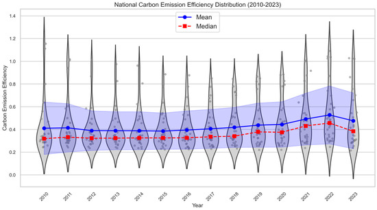
Figure 1.
Nationwide distribution of CEE: 2010–2023. Note: Violin plots display the distribution of provincial efficiency values (n = 30 provinces) computed from the Super-SBM model with undesirable outputs under variable returns to scale. The blue shaded area represents the 95% confidence interval of the national mean carbon emission efficiency, and the grey dots denote individual provincial observations for each year. All efficiency values are dimensionless.
Over 2010–2023, China’s national carbon-emission efficiency exhibits a nonlinear path characterized by four phases: initial easing, subsequent gradual recovery, faster gains after the pandemic, and a retreat in 2023. The national mean and median moved downward in 2010–2015; during 2016–2018 they edged up, reflecting the post-Paris strengthening of emission-control measures [1] and structural reforms, including capacity reduction. A declining coal share and rising proportions of natural gas and renewables materially improved efficiency. The period 2019–2022 saw a pronounced upswing, peaking in 2022, likely due to pandemic-induced slowdowns in industry and transport that lowered energy consumption and emissions. China’s 2020 announcement of the “2030 carbon peak/2060 carbon neutrality” targets also reinforced the shift toward higher efficiency. In 2023, efficiency softened yet remained above earlier levels, which may be attributed to the post-“dynamic zero-COVID” rebound in mobility and industrial operations—together with moderate GDP recovery—raising fossil-energy use and emissions.
Across all years, the mean exceeds the median, indicating that a small set of high-efficiency provinces persistently pulls up the national average, while most provinces cluster in the mid-to-low efficiency range. From the widths of the violins and their confidence bands, dispersion contracted during 2013–2016, but widened in 2020–2022 with an elongated upper tail—signaling stronger top performers and heightened segmentation. In 2023, dispersion narrowed slightly yet showed no clear convergence. The mean and median rose in tandem in 2019–2020, implying broad-based improvements; both declined in 2022–2023, suggesting a risk of efficiency give-back amid economic normalization and the rebound of energy consumption. Overall, national efficiency is higher than a decade ago, but the gains are disproportionately driven by frontier provinces; median improvement and dispersion convergence remain limited.
Using a Super-SBM model with undesirable outputs, we compute the carbon-emission efficiency of 30 Chinese provinces for 2010–2023; the results are reported in Table 4.
Table 4.
Provincial CEE from 2010 to 2023.
From a provincial perspective, CEE displays pronounced regional disparities and remains unevenly distributed. Provinces along the coast tend to achieve higher efficiency, as intensive factor inputs yield superior economic outcomes and indicate a more sustainable development trajectory. Continued economic expansion has provided additional resources for environmental remediation and governance in these areas. Against the backdrop of increasingly stringent environmental regulation, the central–western region has gradually strengthened, with aggregate efficiency improving. To analyze the spatiotemporal distribution of CEE over 2010–2023, we partition provinces into four categories—low, mid-low, mid-high, and high—via the Jenks natural breaks approach, as shown in Figure 2.
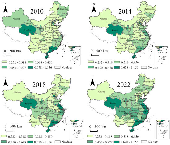
Figure 2.
Spatial distribution of provincial CEE in China, 2010–2023. Note: Produced on the basis of the standard map number GS (2020)4619, downloaded from the standard map service website of the Ministry of Natural Resources of China. The maps are strictly data-driven, without interpolation or smoothing. All color palettes and legends are consistent across panels, and efficiency values are dimensionless.
Provinces with low average carbon-emission efficiency during 2010–2023 are Hebei, Shanxi, Inner Mongolia, Liaoning, Jilin, Heilongjiang, Henan, Guangxi, Guizhou, Yunnan, Shaanxi, and Xinjiang. Compared with coastal counterparts, these jurisdictions show weaker economic activity yet retain a high concentration of energy-intensive production and a fossil-fuel-centric energy mix, forming a “low-activity–high-energy-use–high-emission” pattern. The heavy-industry bases—Hebei, Shanxi, Inner Mongolia, and Shaanxi—remain heavily dependent on heavy manufacturing, with an extensive, resource-consuming growth style that breeds high energy intensity and pollution. In the Northeast (Liaoning, Jilin, Heilongjiang), a high proportion of legacy processes and equipment, limited penetration of advanced energy-saving/low-carbon upgrades, and cold-season conditions that elevate heating demand—together with population loss and shrinking demand—jointly suppress efficiency. For Guizhou, Yunnan, and Xinjiang, low efficiency is closely tied to extensive growth trajectories and the incomplete maturation of energy-conservation and emission-reduction technologies.
Provinces with lower-middle carbon-emission efficiency include Anhui, Fujian, Jiangxi, Shandong, Hubei, Hunan, Chongqing, Sichuan, and Gansu. In the central region (Anhui, Hubei, Hunan, Jiangxi), dense populations and manufacturing agglomerations within urban clusters—reinforced by the “Rise of Central China” strategy—have spurred infrastructure expansion and mid-stream manufacturing, markedly raising the scale and intensity of primary energy consumption. Growth thus remains energy-dependent, and the economy–environment alignment is weak. Limits in production and energy management, together with insufficient R&D and deployment of green technologies, keep efficiency at a lower-middle level and make near-term gains difficult.
As one of the country’s largest industrial bases, Shandong exhibits high unit energy use while specializing in intermediates and primary materials; relatively low value added per unit energy constrains efficiency improvements. In the Sichuan–Chongqing corridor, complex topography elevates transport energy demand, and electricity-driven, energy-intensive industries are concentrated; although abundant hydropower reduces emission intensity, under the SBM framework input growth has outpaced desirable output, so overall efficiency has not improved. In Fujian, a high share of mountainous and hilly terrain raises transport energy costs; the energy mix retains a rigid coal-power component, and process management and green practices require upgrading, jointly depressing efficiency. Gansu is resource-oriented and positioned upstream in processing, showing an asymmetry of “local emissions with exported value added”; water scarcity in its arid climate raises abatement-related water costs, making short-run efficiency gains hard to achieve.
Tianjin, Shanghai, Jiangsu, Zhejiang, and Ningxia fall into the upper-middle efficiency category. These jurisdictions are progressively reconciling economic performance with environmental protection, achieving relatively high efficiency. In the Yangtze River Delta, privileged geography and early industrialization/marketization have produced a comprehensive development platform. Lower reliance on primary energy, faster industrial restructuring, and the extension of manufacturing toward high-tech segments and modern services jointly raise energy-adjusted output. Backed by national policy instruments, regional systems for energy conservation and emissions control have matured quickly; openness and vibrant private enterprise facilitate rapid technology introduction and upgrading. The YRD therefore, exhibits synergistic gains from technological progress and structural upgrading and is positioned to furnish tailored green, low-carbon technical assistance to other regions. Tianjin’s port-centric, modern-manufacturing structure around the Binhai New Area enhances factor and energy efficiency; the scaling of electronics and related sectors lifts energy productivity, yielding a steady upper-middle efficiency level. Ningxia, serving as a northwest energy hub, has deployed wind and photovoltaic resources at scale, enabling local absorption and cross-regional transmission of clean power; the accelerated shift toward a low-carbon primary energy mix underpins its comparatively high efficiency.
The high-efficiency group includes Beijing, Guangdong, Hainan, and Qinghai. Average scores are >0.70, with some provinces exceeding 1.00 in recent years, marking frontier performance. Beijing leads by virtue of a tertiary-sector-dominated structure, vibrant innovation capacity, and strong human-capital magnetism. Hainan’s tourism-led economy and growing deployment of green, clean energy offer a solid platform for the “dual-carbon” agenda. Qinghai’s endowment of wind and solar resources has made it a hub for clean-energy development, catalyzing a transition from fossil-centric consumption. Guangdong, centered on the Pearl River Delta, features rapid structural upgrading and service-sector expansion; the electronics, high-end equipment, and modern-services clusters contribute materially to growth, combined with technological upgrading and managerial efficiency, this keeps provincial CEE at a high level.
5.1.2. Measurement and Analysis of CEE in Eight Comprehensive Economic Zones
The State Council Development Research Center divides China into eight comprehensive economic zones: the Northern Coastal, which includes Beijing, Tianjin, Hebei, and Shandong; the Eastern Coastal, which includes Shanghai, Jiangsu, and Zhejiang; the Southern Coastal, which includes Fujian, Guangdong, and Hainan; the Northeast, which includes Jilin, Liaoning, and Heilongjiang; the Central Yellow River, which includes Shaanxi, Shanxi, Henan, and Inner Mongolia; the Central Yangtze River, which includes Hubei, Hunan, Jiangxi, and Anhui; the Southwest, which includes Guangxi, Yunnan, Guizhou, Sichuan, and Chongqing; and the Northwest, which includes Gansu, Qinghai, Ningxia, and Xinjiang (Tibet is not included). To better analyze the differences and trends in CEE across regions from 2010 to 2023, this study calculates the average CEE for the entire country and the eight economic zones, as shown in Table 5, and presents the results in a line chart, as shown in Figure 3.
Table 5.
CEE of eight comprehensive economic zones.
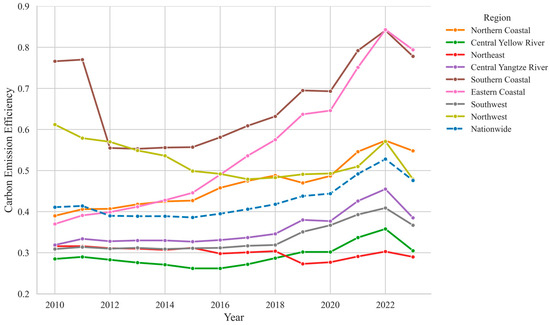
Figure 3.
Temporal evolution of CEE across eight comprehensive economic zones (2010–2023). Note: Lines represent zone-level mean efficiency scores, computed as the arithmetic average of provincial CEE values within each zone (n = 30 provinces total). All values are unitless efficiency scores derived from the Super-SBM model. Solid lines indicate mean trends.
To further demonstrate the spatial heterogeneity of China’s carbon emission efficiency (CEE), this section examines the temporal evolution and regional disparities across the eight comprehensive economic zones from 2010 to 2023. During 2010–2014, national and most regional CEE remained broadly stable, with slight declines in the Central Yellow River and Northeast regions, indicating that periods of rapid economic growth were still accompanied by high carbon intensity. The Southern Coastal region experienced a marked drop—from 0.766 to 0.556—likely reflecting heavy reliance on investment- and export-led growth, the rapid expansion of energy-intensive manufacturing, and an energy mix still dominated by coal and oil. In the early stage of conservation and abatement policies, development priorities remained growth-oriented and policy effects had yet to materialize, thereby constraining efficiency gains. In 2015–2019, efficiency improved across the Eastern Coastal and the Southern Coastal, closely aligned with supply-side structural reforms and the rollout of energy-saving policies. From 2020 to 2022, under the joint influence of the pandemic and the carbon-neutrality pledge, CEE rose rapidly nationwide (Southern Coastal 0.841, Eastern Coastal 0.843 in 2022). A modest pullback occurred in 2023 across most regions, pointing to rebound pressures in energy use during post-pandemic recovery. The pandemic period also revealed the resilience of developed coastal economies, where digital transformation and green-technology investment mitigated efficiency losses.
During 2010–2023, the Eastern and Southern Coastal regions consistently outperformed the national CEE average, attaining 0.843 and 0.841 in 2022. Their advantage reflects coordinated progress in industrial restructuring, efficient energy use, and the expansion of clean energy and high-tech sectors. CEE in the Northern Coastal and Northwest regions exceeded the national mean, the former reached 0.573 in 2022. After a mid-decade dip from resource and energy intensive expansion, the Northwest rebounded post 2020 with new energy rollout and policy support. Yangtze Central and the Southwest remained near the national mean with steady gains, aided by upgrading and conservation policies (Yangtze) and plentiful renewable resources (Southwest); however, large heavy-industry shares keep their efficiency below that of the southeastern coast. The Yellow River Central and Northeast zones consistently occupied the lower tail with limited variability, indicative of heavy industrial structures and strong dependence on high-carbon fuels.
In sum, pronounced CEE disparities across the eight comprehensive economic regions likely arise from uneven regional development, differences in industrial structure, and divergent energy mixes; advancing the low-carbon transition calls for focusing on low-efficiency regions with substantial abatement potential.
In sum, pronounced CEE disparities across the eight comprehensive economic regions likely stem from uneven regional development, differences in industrial structure, and divergent energy mixes. These differentiated trajectories provide empirical evidence for the study’s dual-scale analytical framework, demonstrating that national averages often conceal substantial inter-regional heterogeneity in technological progress and energy transition. To advance China’s low-carbon transformation, region-specific policy design—focusing on industrial upgrading, clean-energy expansion, and technological innovation in low-efficiency zones—is essential for achieving balanced and sustainable efficiency improvements nationwide.
5.2. Dynamic Analysis of CEE Changes
5.2.1. Dynamic Analysis of Provincial CEE Changes
The CEE calculated using the super-efficient SBM model based on undesirable outputs represents a static analysis, but its results do not reflect the changes in CEE over time. The efficiency measurement based on the ML index allows for dynamic analysis of the growth rate of CEE in different years, helping to clarify the changes in CEE and the roles of technical efficiency and technological progress in productivity [57].
MATLAB is used in this study to calculate the ML index and its decomposition values for 30 provinces in China from 2010 to 2023. The ML index represents a dynamic change rate compared year by year, with 2010 as the base year. The index change between 2011 and 2010 constitutes the first data group, and subsequent years follow the same pattern. Due to space limitations, only the CEE change index and its decomposition indices for 2010–2011, 2014–2015, 2018–2019, and 2022–2023 are presented, as shown in Table 6.
Table 6.
ML index and decomposition of eight comprehensive economic zones.
The ML index was approximately 1 during 2011–2014 (Figure 4), suggesting minor fluctuations around a stable efficiency level and limited contributions from EC and TC. Over 2015–2018, TC persistently exceeded 1—nearing 1.03 in 2017–2018—even as EC weakened intermittently, implying technology-led progress consistent with supply-side structural adjustments and the green-development strategy. The years 2019–2022 saw sustained improvement (ML > 1): although EC fell to 0.937 in 2019, TC rose to 1.121, ensuring net gains, and both EC and TC were positive in 2021–2022. In 2023, ML dropped to 0.894, with EC and TC simultaneously below 1, indicating a significant pullback potentially tied to the rebound of high energy-use industries during economic normalization and to external energy-price shocks. Overall, TC has been the primary driver of efficiency improvement, whereas EC has lagged. The decomposition results further indicate that EC captures widespread but modest catch-up effects, while TC represents outward shifts of the production frontier with stronger aggregate impacts. Therefore, technological progress remains the dominant source of national CEE growth, suggesting that future improvements should combine continued innovation with enhanced managerial efficiency and more effective factor allocation.
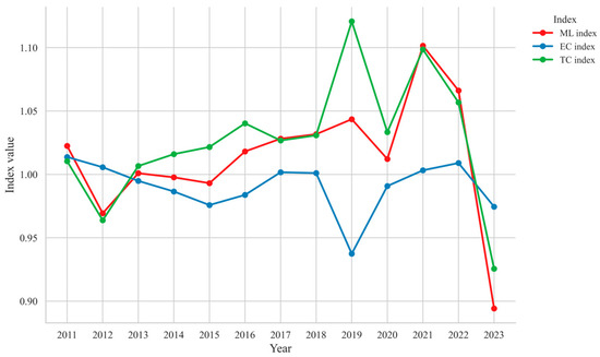
Figure 4.
Decomposition trend of the ML index of CEE from 2010 to 2023.
At the provincial level, pronounced differences emerge in the evolution of CEE and in the contribution structure of EC versus TC. Provinces can be grouped as follows.
- TC-led type, Coastal—Beijing, Shanghai, Jiangsu, Zhejiang, Guangdong: efficiency gains are primarily propelled by TC, with EC providing supportive co-movements.
- Structural-upgrade type, Central—Anhui, Fujian, Jiangxi, Shandong, Henan, Hubei, Hunan: during 2018–2019, TC dominated due to industrial upgrading and process retrofits; in 2022–2023, an energy-use rebound coincided with simultaneous declines in both TC and EC.
- Allocation-constrained type—Tianjin, Hebei, Liaoning, Jilin, Heilongjiang: weak governance and factor-allocation efficiency limit sustained improvement; episodic TC upticks have not translated into durable gains.
- Resource-dependent type—Shanxi, Inner Mongolia, Shaanxi, Gansu, Ningxia, Xinjiang: many operate upstream in resource-intensive and process industries; EC is persistently weak and TC improvements have not yielded lasting efficiency upgrades.
- TC-driven but unstable type, Southwest —Sichuan, Chongqing, Guizhou, Yunnan: TC raised efficiency in 2018–2019, yet the momentum proved hard to maintain; widespread shortfalls in managerial and allocation efficiency (low EC) meant that 2022–2023 combined external shocks with internal bottlenecks, producing volatile gains.
- Structure-sensitive type, Small-scale—Hainan, Qinghai: small economic size and narrow industrial bases heighten the risk of TC–EC mismatches, leading to fluctuation in the ML index.
5.2.2. Dynamic Analysis of CEE Changes in the Eight Comprehensive Economic Zones
Carbon-emission efficiency in China’s eight comprehensive economic zones displays distinct regional signatures. We employ the Malmquist–Luenberger (ML) index to perform an intertemporal evaluation for 2011–2023. Summary estimates are provided in Table 7, and Figure 5 depicts the annual ML distribution for each region.
Table 7.
Decomposition of the ML index of CEE in the eight comprehensive economic zones.
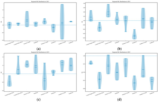
Figure 5.
Decomposition trends of the ML index of CEE in the eight comprehensive economic zones from 2010 to 2023: (a) year 2011; (b) year 2015; (c) year 2019; (d) year 2023.
In cross-regional comparison, the Eastern and Southern Coastal regions have long led in performance; their ML indices reached 1.112 and 1.106 in 2018–2019, driven primarily by technical change (TC). Both, however, fell back in 2022–2023, indicating pressure from the return of carbon-intensive activities. The Northern Coastal region posted relatively high efficiency in 2010–2011 but then trended downward, dropping to 0.943 in 2018–2019, largely due to efficiency deterioration (EC < 1). The central belt is heterogeneous: the Yangtze Central and Yellow River Central areas improved in 2018–2019 on the back of TC, yet recorded the steepest declines in 2022–2023, underscoring heavy dependence on green technologies. The Southwest performed strongly in 2018–2019 (ML = 1.097, TC = 1.116), reflecting extensive hydropower use, but also slipped in 2022–2023. The Northwest has remained structurally weak, constrained by resource dependence and low energy efficiency. The Northeast stayed at the lower end, falling to 0.903 in 2018–2019 mainly due to EC deterioration; despite some rebound in 2022–2023, overall efficiency remains inadequate.
From a within-region perspective, the Eastern and Southern Coastal zones combine higher overall efficiency with smaller intra-regional variance, reflecting the effects of industrial upgrading and technological spillovers; nevertheless, 2022–2023 saw efficiency weaken and dispersion widen in both zones. The Northern Coastal region has undergone a sustained efficiency decline alongside growing internal heterogeneity. The central region registered gains in 2018–2019, but both aggregate performance and within-region dispersion deteriorated in 2022–2023. After a period of stability, the Southwest has also softened. The Northwest and Northeast continue to underperform, with persistent within-group gaps; some convergence is evident in the Northwest, while the Northeast’s enduring inefficiency is linked to structural rigidities.
The eight comprehensive economic zones display significant inter-regional divergence. The southeast coast maintains leadership via structural upgrading and innovation; central and southwestern regions achieve policy-induced yet fluctuant advances; the northern coast and Northeast underperform due to efficiency decay, with limited rebound capacity; and the Northwest hovers at the bottom given resource dependence and structural stickiness. The downturn in 2022–2023 reveals the vulnerability to energy-intensive resurgence during recovery, implying that further improvement requires not only the continuation of TC but also reinforced EC and institutional enforcement. Intra-regional inequality is uneven: Eastern/Southern Coastal areas—historically high-performing with narrow spreads—now exhibit wider dispersion; Northern Coastal weakness coincides with greater internal variance; the Central region transitions from overall uplift to concurrent declines in average performance and within-region cohesion; the Southwest shifts from stability toward mild internal differentiation; the Northwest shows some narrowing of gaps, whereas the Northeast remains durably imbalanced due to structural rigidity. On balance, national gains have been TC-driven but strongly region-specific; consolidating TC while enhancing EC, strengthening enforcement, curbing energy-intensive rebound, and fostering within-region convergence should be central to the next phase.
6. Drivers of China’s CEE and Forecasts
6.1. Historical-Stage Analysis of Influencing Factors (2010–2023)
The empirical assessment employs a Tobit specification, with CEE as the dependent variable and the candidate drivers as explanatory variables, estimated both nationally and for each of China’s eight comprehensive economic zones. Variance inflation factors (VIFs) for all regressors are below 5.5, indicating that multicollinearity is not a concern [58]. The full results are presented in Table 8.
Table 8.
Tobit model regression results.
Results from the Tobit regressions reveal that technological advancement is a robust positive determinant of CEE at the national level, with especially salient effects in the Northern Coastal and Central Yangtze regions. While economic development is generally associated with higher efficiency, the relationship is region-specific: in the Northwest and Northeast, the coefficient turns negative, indicating a nonlinear EKC-type pattern. Optimization of industrial structure—through the expansion of services and high-value activities—significantly improves CEE, particularly in the Eastern Coastal and Central Yangtze regions. However, in the Central Yellow River and Northeast, the coefficient becomes negative, suggesting that service sector expansion remains concentrated in resource-dependent or energy-intensive segments, which do not substantially reduce emissions. Without simultaneous upgrading of the secondary sector, overall efficiency gains remain constrained.
Environmental protection expenditure shows a positive association with CEE nationally and in regions such as the Southwest and Central Yellow River, indicating that fiscal spending can serve as an effective environmental policy instrument. Conversely, the negative coefficient in the Central Yangtze region may reflect policy lag or implementation inefficiency. Population density exhibits an overall negative association with CEE, suggesting that excessive urban concentration raises emission intensity and strains resources and the environment. However, positive effects in the Southwest and Northeast indicate that moderate agglomeration can facilitate green infrastructure and centralized abatement.
Energy consumption is negatively related to CEE nationwide, yet turns positive in the Eastern and Southern Coastal regions, where cleaner power portfolios mitigate the adverse impact of energy use. Environmental regulation is insignificant nationally but negative in the Central Yellow River and Central Yangtze regions—consistent with end-of-pipe, cost-intensive regulatory patterns and limited coordination between national and local implementation. Government intervention exhibits mixed effects: weakly positive on average, but negative in the Eastern Coastal, Northeast, and Northwest regions. This suggests nonlinear or diminishing returns in high-tech, capital-intensive contexts and possible crowding-out of private investment in state-led economies. Limited enforcement technologies and governance capacity further constrain the green transition.
Urbanization shows heterogeneous effects—statistically insignificant overall, but negative in the Northern Coastal and Northwest, likely reflecting infrastructure constraints and lagging public-transit or heating systems that increase emission intensity. FDI is insignificant nationally but positive in Southern Coastal, Northern Coastal, and Central Yangtze regions, where foreign firms bring cleaner technologies and managerial spillovers. By contrast, negative FDI effects in the Northeast and Southwest indicate pollution transfer toward provinces with weaker environmental governance.
To address potential endogeneity between CEE and its determinants, a Tobit model incorporating one-period lagged regressors and Mundlak provincial mean terms was additionally estimated. The full results are presented in Table 9.
Table 9.
Tobit robustness analysis.
Endogeneity may arise because policy, structural, and technological variables are likely to be jointly determined with CEE. The lagged specification mitigates reverse causality, as current efficiency cannot influence the previous year’s covariates. In parallel, the Mundlak adjustment controls for time-invariant unobserved heterogeneity, including geographical endowment, institutional setting, and long-term development trajectories.
The Lagged–Mundlak Tobit results remain directionally and economically consistent with those of the baseline Tobit model. Technological development, environmental investment, industrial upgrading, and economic development continue to exhibit significant positive effects, whereas energy consumption and population density persist as negative determinants. Although significance levels slightly decline for certain regressors in the lagged specification, the overall directions and magnitudes are stable, indicating robust and reliable estimates.
Overall, the baseline Tobit model provides stable and interpretable results, while the Lagged–Mundlak specification confirms that potential endogeneity does not materially bias the estimated relationships. Consequently, the baseline Tobit is retained as the main empirical specification, with the Lagged–Mundlak Tobit serving as a robustness validation.
6.2. ARIMA-LSTM Based Forecasts of CEE in China
In view of the publication lag of official statistics, this study employs a hybrid ARIMA–LSTM model to generate short-term forecasts (2024–2025) of China’s CEE and its key influencing factors. The forecasts aim to characterize near-term trends and provide an empirical basis for evaluating policy progress. The 14th Five-Year Plan period (2021–2025) represents the formative stage of China’s “dual-carbon” strategy and a critical window for achieving peak emissions. It is also a pivotal phase for industrial upgrading and the transition toward green and low-carbon development. Focusing on this interval enables cross-regional comparison and offers forward-looking policy insights, helping to track the national decarbonization trajectory and the evolving dynamics of regionally coordinated development.
Provincial CEE data are first standardized (Z-score) to harmonize scales and stabilize training. Each province’s time series is then subjected to formal stationarity diagnostics before ARIMA specification. Both the Augmented Dickey–Fuller (ADF) and Kwiatkowski–Phillips–Schmidt–Shin (KPSS) tests were applied to the level and first-difference series, supplemented by Ljung–Box tests on residual autocorrelation. The results show that most series are non-stationary in levels but become stationary after first differencing, confirming an integration order of one (d = 1).
Model orders (p, q) for the ARIMA component were chosen through a combination of AIC/BIC information criteria, and Ljung–Box tests to ensure residual white noise. These diagnostics consistently supported ARIMA (3, 1, 2) as the most parsimonious and stable specification across provinces. One provincial series marginally violated the KPSS stationarity condition (p < 0.05) even after first differencing; however, its ADF statistics and residual correlograms indicated weak trend-stationary behavior rather than explosive non-stationarity. To maintain cross-provincial comparability, d = 1 was retained for this case, as higher differencing (d = 2) did not improve model fit or forecasting accuracy. These diagnostic-based procedures ensure that the differencing and order selection are both empirically grounded and reproducible.
To capture both linear and nonlinear dynamics in the evolution of CEE, a residual-correction hybrid framework is constructed. The linear component is modeled using the ARIMA (3, 1, 2) process to capture deterministic trends and autocorrelations, while the nonlinear residuals from ARIMA are modeled by a single-layer LSTM network with 32 hidden units. Before training, residuals are standardized (mean = 0, variance = 1) and subsequently re-scaled to the original units after forecasting.
The five-year look-back window is selected based on both empirical and contextual considerations. Empirically, the autocorrelation and partial autocorrelation analyses of the residual series indicate that predictive information decays rapidly beyond five lags, suggesting that longer windows would introduce noise rather than informative structure. Contextually, a five-year span aligns with China’s medium-term economic and policy cycles—particularly the “Five-Year Plan” period—capturing structural and technological adjustments that evolve at this horizon. Therefore, the chosen window length provides a balanced and parsimonious configuration that effectively captures temporal dependencies while minimizing overfitting risk, particularly given the limited annual sample size (2010–2023).
The LSTM network adopts a lightweight design:
- Input layer—sliding window of five observations (the most recent five residuals) to predict the next period;
- LSTM layer—one recurrent layer with 16–32 hidden units, capturing short-term fluctuations and long-range dependencies;
- Fully connected (FC) layer—projects the hidden representation to a single scalar output;
- Output layer—one-step-ahead residual forecast.
Training uses the Mean Squared Error (MSE) loss function and the Adam optimizer (learning rate = 0.01). Regularization techniques include dropout = 0.2, L2 weight decay = 1 × 10⁻⁴, gradient clipping (max-norm = 1.0), and an early-stopping mechanism (patience = 20). Samples are generated using a sliding-window design, and training employs a time-ordered 80/20 train–validation split to preserve temporal causality. The model is trained for 300 epochs, after which the predicted ARIMA residual is added to the baseline ARIMA forecast to yield the final prediction.
Leveraging this hybrid ARIMA–LSTM fusion, we forecast provincial CEE for 2024–2025 based on 2010–2023 observations. Supplementary Materials Table S4 compares the forecasting accuracy of the hybrid model with a single ARIMA benchmark across major driving factors. The hybrid model achieves consistently lower MAE values for nearly all variables, demonstrating superior predictive performance—particularly for nonlinear or complex time-series patterns—while only the industrial-structure variable shows marginally better results under the pure ARIMA specification.
As shown in Figure 6, China’s provincial CEE during 2021–2025 exhibits a nationally increasing trend, while marked cross-provincial differences endure. The eastern seaboard remains at the frontier and continues to strengthen, consistent with structural optimization and wider deployment of clean technologies. The midwestern provinces improve gradually with relatively smooth increments. Inner Mongolia, Heilongjiang, and Shanxi, representing older industrial heartlands, maintain below-average efficiency and modest gains, indicating sustained challenges for low-carbon transition. In sum, although aggregate efficiency is set to improve, uneven regional development remains salient, underscoring the need for tailored emission-reduction strategies.
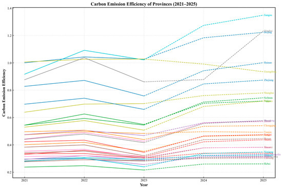
Figure 6.
Provincial CEE in China from 2021 to 2025.
6.3. Future Analysis of Influencing Factors (2024–2025)
Drawing on the preceding Tobit analysis together with the forecasting results, this study conducts a forward-looking assessment of the key factors shaping China’s CCE and benchmarks them against historical influences. Summary evidence is presented in Table 10.
Table 10.
Heterogeneity analysis results.
Comparing the regression results across the historical and prospective periods indicates that, while the underlying mechanism influencing CEE remains broadly stable, several effect sizes shift over time. First, the level of technological development remains the most salient positive determinant in both periods, confirming technological progress as the core driver of efficiency gains. Second, the positive impact of economic development strengthens, suggesting a more compatible relationship between growth and decarbonization efficiency going forward. Third, the beneficial effect of industrial restructuring is stable, underscoring the sustained importance of upgrading the industrial mix.
Results indicate that environmental protection is still positively significant but with a reduced effect size, implying lower marginal payoffs as spending normalizes. Population density and energy consumption intensity continue to exert significant negative influences in both the historical and forward periods; nevertheless, these negatives abate modestly in the outlook period, consistent with the early traction of low-carbon urban infrastructure and energy-structure rebalancing. Looking ahead, neither environmental regulation nor government intervention attains statistical significance—the former highlighting the need to strengthen enforcement, the latter indicating that market forces are increasingly pivotal to emissions reduction. Urbanization level and FDI remain non-significant throughout and diminish further in the forward window, suggesting indeterminate effects on carbon-efficiency gains.
Furthermore, to account for forecast uncertainty, 95% prediction intervals for provincial CEE during 2024–2025 are reported in Supplementary Materials Table S3. Aggregating these provincial results by economic zone shows that, while all regions are expected to improve, the magnitude and stability of gains vary considerably. The Eastern and Southern Coastal zones exhibit higher mean forecasts and narrower confidence bands, reflecting stable and sustained progress supported by technological and industrial upgrading. In contrast, the Northeast and Central Yellow River regions display wider intervals and lower predicted means, indicating slower and more uncertain transitions due to structural and energy constraints. Overall, these forecast patterns are consistent with the Tobit-based results, where stronger effects of technological development and industrial optimization coincide with higher predicted efficiency, confirming that both the forecasting and determinant analyses convey a coherent narrative of technology-driven and regionally differentiated efficiency improvement.
7. Conclusions and Policy Recommendations
7.1. Conclusions
This study employs the Super-SBM model considering undesirable outputs and the ML index to calculate and analyze the CEE across 2010–2023 for 30 provinces. The ARIMA–LSTM framework is applied to project CEE trends for 2024–2025. Additionally, it explores the overall characteristics and evolution trends of CEE for the entire country and the eight comprehensive economic regions. The Tobit model is used to identify and analyze the influencing factors and heterogeneity of CEE for both the national level and regional scales. The key conclusions are as follows:
- Nationally, CEE remains low on average but is rising steadily. During the 14th Five-Year Plan (2021–2025), forecasts indicate continued and stable gains in CEE, albeit with limited magnitude. Notable regional disparities persist across the eight comprehensive economic regions. The Eastern and Southern Coastal zones maintain the highest and still-rising efficiency, while the Northern Coastal and Central Yangtze River regions occupy intermediate positions with sustained energy-use pressures. The Southwest and Northwest show relatively lower efficiency but possess favorable green-resource endowments and significant transition potential. The Northeast and Central Yellow River regions remain at the lower end, exhibiting gradual but limited improvement.
- Regionally, efficiency performance differs mainly due to variations in industrial structure, resource endowments, and energy transition progress rather than distinct technological frontiers. The Eastern and Southern Coastal regions sustain leadership through technological upgrading and industrial optimization, though recent gains have moderated. The Northern Coastal region shows an early-high/late-low trajectory, largely reflecting slowing efficiency improvement. In the Central Yangtze River, efficiency rose during 2018–2019 but declined in 2022–2023 amid economic restructuring pressures. The Southwest improved rapidly in 2018–2019, driven by renewable expansion, then stabilized due to geographic and infrastructure constraints. The Northwest remains constrained by energy intensity and resource dependence, while the Northeast continues to lag due to rigid industrial structures and managerial inefficiency. The Central Yellow River region remains coal-dependent, with slow progress toward transition.
- At the national level, technological development exerts the most consistent and significant positive effect on CEE, confirming technological progress as a sustained driver of improvement rather than a region-specific frontier shift. Economic development and industrial restructuring also show persistent positive impacts, which strengthen in the forecast period, indicating closer coupling between green transformation and efficiency gains. Population density and energy consumption remain significant negative drivers, though their effects gradually moderate with the advancement of green-city and energy-transition policies. Regional heterogeneity in coefficients reflects structural, institutional, and developmental differences, highlighting the need for place-based and differentiated strategies to enhance efficiency and advance coordinated decarbonization.
7.2. Policy Implications
Grounded in the above findings—marked regional heterogeneity and a technology-led improvement pattern—China’s carbon efficiency transition requires regionally differentiated and factor-oriented strategies that align with the drivers identified in this study.
Grounded in the empirical findings—marked regional heterogeneity and a technology-led improvement pattern—China’s CEE transition requires regionally differentiated and factor-oriented strategies aligned with the key drivers identified in this study. The Tobit analysis confirms that technological development (TD), industrial structure (IS), and environmental protection expenditure (EP) exert the strongest positive influences on CEE, while energy consumption (EC) and population density (PD) remain significant negative determinants. These relationships inform the following policy recommendations.
- (1)
- Lead with green innovation. Technological innovation is verified as the most influential positive driver of CEE at both national and regional levels. Eastern and southern coastal regions, already innovation-intensive, should further integrate research and application, promote the commercialization of clean technologies in the energy, transport, and construction sectors, and strengthen intellectual property protection to sustain innovation-driven growth. Lagging regions such as the Northeast and Central Yellow River should expand fiscal and credit incentives for low-carbon technology adoption. Targeted R&D subsidies, preferential tax treatment, and talent programs can help accelerate technological diffusion and narrow regional gaps.
- (2)
- Fuse growth with low-carbon transition. Economic development remains a statistically significant and stable contributor to efficiency, suggesting that growth and decarbonization can advance in parallel when driven by green investment and productivity improvement. Policymakers should maintain steady growth while continuously upgrading the industrial structure. Encouraging the expansion of modern services, high-value manufacturing, and circular-economy industries can replace energy- and emission-intensive sectors. Compact, transit-oriented, and green urban development will further mitigate efficiency losses in high-density areas. Integrating industrial restructuring with sustainable urbanization will accelerate the shift from resource-driven to innovation-driven growth.
- (3)
- Optimize industrial structure. The Tobit results identify industrial upgrading as the second most important positive determinant of CEE. Regions dominated by heavy industry should accelerate structural transformation and promote cleaner production. Implementing capacity replacement and emission control mechanisms for sectors such as steel, cement, and chemicals, alongside fiscal rebates or low-interest loans for firms meeting energy-intensity and emission targets, can generate tangible efficiency gains. These measures will gradually shift local economies toward a cleaner, more efficient industrial system.
- (4)
- Accelerate energy-mix transition. Energy consumption exerts a significant negative effect on efficiency, underscoring the need to reduce fossil dependency. Expanding renewable energy capacity and improving grid integration—especially in the Southwest and Northwest—will strengthen CEE over time. Dynamic energy pricing, carbon budgets, and performance-linked fiscal incentives should reward conservation and penalize inefficiency. Integrating energy-saving indicators into local government evaluations will reinforce accountability and ensure the long-term sustainability of efficiency gains.
- (5)
- Promote sustainable urbanization and population balance. Population density shows a robust negative relationship with CEE, implying that excessive urban concentration strains resources and increases emission intensity. Advancing a new type of urbanization supported by green infrastructure, smart mobility, and low-carbon buildings is thus essential. Balanced population and industrial distribution through metropolitan–county coordination can reduce congestion and energy waste. Improved urban planning standards integrating land use, transportation, and environmental management will help alleviate efficiency losses from over-urbanization.
- (6)
- Raise the quality of foreign direct investment. Although the national-level coefficient for FDI is statistically insignificant, regional results indicate positive effects in innovation-oriented regions (e.g., Southern and Northern Coasts) but negative spillovers in areas with weaker environmental governance. Hence, FDI should be reoriented toward high-tech and clean industries through tax incentives, green finance, and performance-based evaluation. Encouraging localized R&D and international cooperation on low-carbon technologies will enhance both technological upgrading and regional convergence in carbon efficiency.
- (7)
- Strengthen governance and coordination. Effective carbon governance requires coherent multi-level coordination. Integrating carbon-efficiency targets into fiscal performance, planning, and environmental assessments ensures policy alignment. The Tobit analysis underscores the growing importance of institutional and governance quality, reflected in the moderate but positive coefficient of government intervention. Strengthening the carbon-inclusive mechanism that links enterprises and individuals to emission-reduction incentives, promoting inter-regional carbon trading, and enhancing digital monitoring will further reinforce governance-driven efficiency improvement.
Collectively, these evidence-based measures constitute a coherent framework for enhancing CEE under China’s dual-carbon strategy. By quantitatively linking each lever to the direction and magnitude of its empirical impact, the policy roadmap aligns with the econometric results while acknowledging regional heterogeneity. Coordinated technological innovation, structural transformation, and governance reform together form the practical pathway toward balanced and sustainable carbon-efficiency improvement.
7.3. Limitations and Future Research
This study has several limitations. Although the dataset mainly originates from official statistical yearbooks, minor inconsistencies and occasional missing data may introduce measurement uncertainty. Linear interpolation (<2% of observations) was applied to preserve time-series continuity, which may smooth short-term variation. The limited sample period (2010–2025) constrains the depth of time-series learning and the robustness of panel regressions. Tobit coefficients reflect statistical associations rather than causal effects and should be interpreted accordingly. The Super-SBM model assumes a unified national frontier to ensure comparability, but potential regional technological heterogeneity remains unmodeled. Future research could extend this framework using meta-frontier or zone-specific DEA models, incorporate longer time spans and city-level data, and combine causal inference approaches to enhance robustness and policy relevance.
Supplementary Materials
The following supporting information can be downloaded at: https://www.mdpi.com/article/10.3390/su172210007/s1, Table S1. Stationarity Test and ARIMA Model Diagnosis Results of CEE Series by Province; Table S2. The 95% CIs for ML, EC, and TC for each province under 1000 Bootstramps; Table S3. The 95% Cis of CEE for each province under 1000 Bootstramps; Table S4. Comparasion between ARIMA and Hybrid Model; Table S5. FDI; Table S6. GI; Table S7. IS; Table S8. TD; Table S9. EP; Table S10. EC; Table S11. ER; Table S12. UR; Table S13. PD; Table S14. ED.
Author Contributions
Conceptualization, methodology, data curation, formal analysis, writing—original draft preparation, Y.S.; review and editing, supervision, H.L. All authors have read and agreed to the published version of the manuscript.
Funding
This research received no external funding.
Institutional Review Board Statement
Not applicable.
Informed Consent Statement
Not applicable.
Data Availability Statement
All data and models generated or used in the research process of this paper are presented and explained in the body of the article.
Conflicts of Interest
The authors declare no conflicts of interest.
Abbreviations
The following abbreviations are used in this manuscript:
| CEE | Carbon Emission Efficiency |
| SBM | Slack-Based Measure |
| ML | Malmquist-Luenberger |
| ARIMA | Autoregressive Integrated Moving Average |
| LSTM | Long Short-term Memory |
| TD | Technological Development |
| ED | Economic Development |
| IS | Industrial Structure |
| EP | Environmental Protection |
| FDI | Foreign Direct Investment |
| EC | Energy Consumption |
| GI | Government Intervention |
| UR | Urbanization |
| VIF | Variance Inflation Factor |
References
- Lucey, B.M.; Urquhart, A.; Vigne, S.A. Why the global economy is more uncertain than ever, and what to do about it. Nature 2025, 643, 634–637. [Google Scholar] [CrossRef] [PubMed]
- Ning, L.C.; Zheng, W.; Zeng, L.E. Research on China’s Carbon Dioxide Emissions Efficiency from 2007 to 2016: Based on Two Stage Super Efficiency SBM Model and Tobit Model. Beijing Da Xue Xue Bao 2021, 57, 181–188. [Google Scholar]
- Ma, Y.; Zhang, Z.; Yang, Y. Calculation of CEE in China and analysis of influencing factors. Environ. Sci. Pollut. Res. 2023, 30, 111208–111220. [Google Scholar] [CrossRef] [PubMed]
- Qin, Y.X.; Huang, R. CEE and influencing factors in Central and Eastern European countries based on Super-SBM model. Adv. Clim. Change Res. 2024, 20, 581. [Google Scholar]
- Kaya, Y.; Yokobori, K. Environment, Energy, and Economy: Strategies for Sustainability; United Nations University Press: Tokyo, Japan, 1997. [Google Scholar]
- Mielnik, O.; Goldemberg, J. The evolution of the “carbonization index” in developing countries. Energy Policy 1999, 27, 307–308. [Google Scholar] [CrossRef]
- Ang, B.W. Is the energy intensity a less useful indicator than the carbon factor in the study of climate change? Energy Policy 1999, 27, 943–946. [Google Scholar] [CrossRef]
- Shrestha, R.M.; Timilsina, G.R. Factors affecting CO2 intensities of power sector in Asia: A Divisia decomposition analysis. Energy Econ. 1996, 18, 283–293. [Google Scholar] [CrossRef]
- Fan, Y.; Liu, L.-C.; Wu, G.; Tsai, H.-T.; Wei, Y.-M. Changes in carbon intensity in China: Empirical findings from 1980–2003. Ecol. Econ. 2007, 62, 683–691. [Google Scholar] [CrossRef]
- Oda, J.; Akimoto, K. Carbon intensity of the Japanese iron and steel industry: Analysis of factors from 2000 to 2019. J. Clean. Prod. 2022, 345, 130920. [Google Scholar] [CrossRef]
- Lin, Y.; Huang, J.; Li, M.; Lin, R. Does lower regional density result in less CO2 emission per capita? Evidence from prefecture-level administrative regions in China. Environ. Sci. Pollut. Res. 2022, 29, 29887–29903. [Google Scholar] [CrossRef]
- Wurlod, J.D.; Noailly, J. The impact of green innovation on energy intensity: An empirical analysis for 14 industrial sectors in OECD countries. Energy Econ. 2018, 71, 47–61. [Google Scholar] [CrossRef]
- Li, Y.; Li, J.; Wang, W.; Huang, Q. The Impact mechanism of Global value chain embedment on CEE: The Belt and Road Initiative Evidence and enlightenment of manufacturing industry in countries along the Route. China’s Popul. Resour. Environ. 2021, 31, 15–26. [Google Scholar]
- Aigner, D.; Lovell, C.A.K.; Schmidt, P. Formulation and estimation of stochastic frontier production function models. J. Econom. 1977, 6, 21–37. [Google Scholar] [CrossRef]
- Herrala, R.; Goel, R.K. Global CO2 efficiency: Country-wise estimates using a stochastic cost frontier. Energy Policy 2012, 45, 762–770. [Google Scholar] [CrossRef]
- Du, K.; Zou, C.Y. Regional disparity, affecting factors and convergence analysis of carbon dioxide emission efficiency in China: On stochastic frontier model and panel unit root. Zhejiang Soc. Sci. 2011, 11, 32–43. [Google Scholar]
- Ramanathan, R. A multi-factor efficiency perspective to the relationships among world GDP, energy consumption and carbon dioxide emissions. Technol. Forecast. Soc. Change 2006, 73, 483–494. [Google Scholar] [CrossRef]
- Maradan, D.; Vassiliev, A. Marginal costs of carbon dioxide abatement: Empirical evidence from cross-country analysis. Rev. Suisse D Econ. Stat. 2005, 141, 377. [Google Scholar]
- Zaim, O.; Taskin, F. Environmental efficiency in carbon dioxide emissions in the OECD: A non-parametric approach. J. Environ. Manag. 2000, 58, 95–107. [Google Scholar] [CrossRef]
- Zeng, L.; Lu, H.; Liu, Y.; Zhou, Y.; Hu, H. Analysis of regional differences and influencing factors on China’s carbon emission efficiency in 2005–2015. Energies 2019, 12, 3081. [Google Scholar] [CrossRef]
- Tone, K. A slacks-based measure of efficiency in data envelopment analysis. Eur. J. Oper. Res. 2001, 130, 498–509. [Google Scholar] [CrossRef]
- Tone, K.; Sahoo, B.K. Degree of scale economies and congestion: A unified DEA approach. Eur. J. Oper. Res. 2004, 158, 755–772. [Google Scholar] [CrossRef]
- Andersen, P.; Petersen, N.C. A procedure for ranking efficient units in data envelopment analysis. Manag. Sci. 1993, 39, 1261–1264. [Google Scholar] [CrossRef]
- Sun, X.M.; Zhang, H.; Wang, G. Evaluation of regional carbon emissions performance based on SE-SBM model: Taking Shandong Province as an example. Ecol. Econ. 2016, 32, 68. [Google Scholar]
- Zhang, M.; Xi, S. Evaluation of carbon emission efficiency of resource-based cities and its policy enlightenment. J. Nat. Resour. 2023, 38, 220–237. [Google Scholar] [CrossRef]
- Wang, S.; Gao, S.; Huang, Y.; Shi, C. Spatio-temporal evolution and trend prediction of urban carbon emission performance in China based on super-efficiency SBM model. Acta Geogr. Sin. 2020, 75, 1316–1330. [Google Scholar]
- Zheng, Y.; Jiang, X.; Xiao, Y. Spatio-temporal Evolution and Trend Prediction of Transport Carbon Emission Efficiency. Environ. Sci. 2024, 45, 1879–1887. [Google Scholar]
- Dong, H.; Guo, X. Research on the Spatio-temporal Evolution Characteristics of Carbon Emission Efficiency in China’s Transportation Industry. East China Econ. Manag. 2023, 37, 70–80. [Google Scholar]
- Hu, S.; Li, S.; Meng, X.; Peng, Y.; Tang, W. Study on regional differences of carbon emission efficiency: Evidence from Chinese construction industry. Energies 2023, 16, 6882. [Google Scholar] [CrossRef]
- Zhang, J.; Zhang, Y.; Chen, Y.; Wang, J.; Zhao, L.; Chen, M. Evaluation of Carbon Emission Efficiency in the Construction Industry Based on the Super-Efficient Slacks-Based Measure Model: A Case Study at the Provincial Level in China. Buildings 2023, 13, 2207. [Google Scholar] [CrossRef]
- Wang, L.; Jia, G. Spatial spillover and threshold effects of high-quality tourism development on carbon emission efficiency of tourism under the “double carbon” target: Case study of Jiangxi, China. Sustainability 2023, 15, 4797. [Google Scholar] [CrossRef]
- Du, Y.; Bai, Y.; Liang, J.; Zhang, C.; Jing, L.; Wang, L.; Zou, J. Comprehensive measurement and influencing factors of carbon emission efficiency of tourism in the Yellow River Basin. Arid Land Geogr. 2023, 46, 2074–2085. [Google Scholar]
- Dong, Q.; Zhong, C.; Geng, Y.; Dong, F.; Chen, W.; Zhang, Y. A bibliometric review of carbon footprint research. Carbon Footpr. 2024, 3, 3. [Google Scholar] [CrossRef]
- Xiao, Y.; Ma, D.; Zhang, F.; Zhao, N.; Wang, L.; Guo, Z.; Zhang, J.; An, B.; Xiao, Y. Spatiotemporal differentiation of carbon emission efficiency and influencing factors: From the perspective of 136 countries. Sci. Total Environ. 2023, 879, 163032. [Google Scholar] [CrossRef]
- Zhou, W.Q.; Nie, M. Regional differences in the efficiency of industrial carbon emissions in China. J. Quant. Tech. Econ. 2012, 9, 58. [Google Scholar]
- Zhao, X.; Li, T.; Duan, X. Spatial and temporal evolution of urban CEE in China. Environ. Sci. Pollut. Res. 2023, 30, 114471–114483. [Google Scholar] [CrossRef] [PubMed]
- Sun, X.; Liu, X. Spatiotemporal evolution and influencing factors of urban CEE in China: Based on heterogeneous spatial stochastic frontier model. Geogr. Res. 2023, 42, 3182–3201. [Google Scholar]
- Xing, P.; Wang, Y.; Ye, T.; Sun, Y.; Li, Q.; Li, X.; Li, M.; Chen, W. Carbon emission efficiency of 284 cities in China based on machine learning approach: Driving factors and regional heterogeneity. Energy Econ. 2024, 129, 107222. [Google Scholar] [CrossRef]
- Xu, Y.; Cheng, Y.; Wang, J.; Liu, N. Spatio-temporal evolution and influencing factors of carbon emission efficiency in low carbon city of China. J. Nat. Resour. 2022, 37, 1261–1276. [Google Scholar] [CrossRef]
- Xu, Y.; Cheng, Y.; Zheng, R.; Wang, Y. Spatiotemporal evolution and influencing factors of carbon emission efficiency in the Yellow River Basin of China: Comparative analysis of resource and non-resource-based cities. Int. J. Environ. Res. Public Health 2022, 19, 11625. [Google Scholar] [CrossRef] [PubMed]
- Zhang, Y.; Xu, X. Carbon emission efficiency measurement and influencing factor analysis of nine provinces in the Yellow River basin: Based on SBM-DDF model and Tobit-CCD model. Environ. Sci. Pollut. Res. 2022, 29, 33263–33280. [Google Scholar] [CrossRef]
- Jin, Y.; Zhang, K.; Li, D.; Wang, S.; Liu, W. Analysis of the spatial–temporal evolution and driving factors of carbon emission efficiency in the Yangtze River economic Belt. Ecol. Indic. 2024, 165, 112092. [Google Scholar] [CrossRef]
- Wang, X.; Shen, Y.; Su, C. Spatial-temporal evolution and driving factors of carbon emission efficiency of cities in the Yellow River Basin. Energy Rep. 2023, 9, 1065–1070. [Google Scholar] [CrossRef]
- Zhang, N.; Sun, F.; Hu, Y. Spatiotemporal evolution, regional differences, and influencing factors of CEE in the Yangtze River Economic Belt. Resour. Environ. Yangtze Basin 2024, 33, 1325–1339. [Google Scholar]
- Zheng, R.; Cheng, Y. Impacts of innovation factor agglomeration on CEE in the Yellow River Basin. Geogr. Res. 2024, 43, 577–595. [Google Scholar]
- Yin, N.; Wang, C.; Yan, P. Provincial CEE and driving factors along the Belt and Road in China under carbon peak and carbon neutrality. Coal Eng. 2022, 54, 182–186. [Google Scholar]
- Li, J.; Huang, X.; Chuai, X.; Sun, S. Spatio-temporal Characteristics and Influencing Factors of Carbon Emissions Efficiency in the Yangtze River Delta Region. Resour. Environ. Yangtze Basin 2020, 29, 1486–1496. [Google Scholar]
- Wang, Z.; Shao, H. Spatiotemporal interactions and influencing factors for carbon emission efficiency of cities in the Yangtze River Economic Belt, China. Sustain. Cities Soc. 2024, 103, 105248. [Google Scholar] [CrossRef]
- Jiang, H.; Yin, J.; Wei, D.; Luo, X.; Ding, Y.; Xia, R. Industrial carbon emission efficiency prediction and carbon emission reduction strategies based on multi-objective particle swarm optimization-backpropagation: A perspective from regional clustering. Sci. Total Environ. 2024, 906, 167692. [Google Scholar] [CrossRef]
- Sheng, K.; Li, X.; Sun, W.; Wang, C. Examining the impacts of network position on urban carbon emissions efficiency in China. Acta Geogr. Sin. 2023, 78, 2864–2882. [Google Scholar]
- Huang, T.; Hu, X.; Chen, S.; Wang, Y.; Zhang, B. Evaluation of the sustainable development level of the Belt and Road countries and its impact factors. China Popul. Resour. Environ. 2020, 30, 27–37. [Google Scholar]
- Dong, H.; Liu, Y.; Zhao, Z.; Tan, X.; Managi, S. Carbon neutrality commitment for China: From vision to action. Sustain. Sci. 2022, 17, 1741–1755. [Google Scholar] [CrossRef]
- Goldsmith, R.W. A perpetual inventory of national wealth. In Studies in Income and Wealth; National Bureau of Economic Research: Cambridge, MA, USA, 1951; Volume 14, pp. 5–73. [Google Scholar]
- Zhang, J.; Zhang, Y. Recalculating the Capital of China and a Review of Li and Tang’s Article. Econ. Res. J. 2003, 7, 2003. [Google Scholar]
- Shan, H.J. Reestimating the capital stock of China: 1952–2006. J. Quant. Tech. Econ. 2008, 10, 17–31. [Google Scholar]
- GB/T 2589-2020; General Rules for Calculation of the Comprehensive Energy Consumption. Standardization Administration of PRC: Beijing, China, 2020.
- Long, L. Eco-Efficiency and Effectiveness Evaluation toward Sustainable Urban Development in China: A Super-Efficiency SBM–DEA with Undesirable Outputs. Environ. Dev. Sustain. 2021, 23, 14982–14997. [Google Scholar] [CrossRef]
- Sinniah, S.; Al Mamun, A.; Md Salleh, M.F.; Makhbul, Z.K.M.; Hayat, N. Modeling the Significance of Motivation on Job Satisfaction and Performance Among the Academicians: The Use of Hybrid Structural Equation Modeling–Artificial Neural Network Analysis. Front. Psychol. 2022, 13, 935822. [Google Scholar] [CrossRef]


Disclaimer/Publisher’s Note: The statements, opinions and data contained in all publications are solely those of the individual author(s) and contributor(s) and not of MDPI and/or the editor(s). MDPI and/or the editor(s) disclaim responsibility for any injury to people or property resulting from any ideas, methods, instructions or products referred to in the content. |
© 2025 by the authors. Licensee MDPI, Basel, Switzerland. This article is an open access article distributed under the terms and conditions of the Creative Commons Attribution (CC BY) license (https://creativecommons.org/licenses/by/4.0/).