This section presents the empirical analysis in four parts. We assemble a balanced city–year panel covering Chinese prefecture-level cities over 2011–2021 (exceeding 280 cities), merging agricultural production accounts, input endowments, and meteorological controls with the Peking University Digital Financial Inclusion Index at the city level. Agricultural total factor productivity is estimated via a stochastic frontier approach, producing time-varying measures of technical efficiency and TFP for each city. Our empirical strategy exploits both cross-city and within-city temporal variation, estimating two-way fixed-effects models with city and year fixed effects and the full set of standard controls.
Studying cities rather than provinces alleviates aggregation bias: provincial aggregates pool heterogeneous agro-ecological zones, production structures, and input quality, potentially attenuating or even reversing the sign of covariate–TFP relationships. City-level data preserve meaningful within-province variation in digital finance penetration and agricultural technology, enabling identification under more comparable institutional, regulatory, and climatic environments. This finer granularity also reduces omitted-variable concerns tied to unobserved provincial composition effects and enhances the credibility of our instrumental-variable strategy, which relies on the net of differential exposure to national digital finance expansion and province-level trends on the focal city.
Section 4.1 describes the measurement of agricultural TFP, including the data sources and the stochastic frontier approach used for estimation.
Section 4.2 specifies the baseline regression model, introduces the control variables, and reports the main results on the relationship between digital finance and agricultural productivity.
Section 4.3 explores the underlying mechanism, focusing on the role of capital misallocation and testing its mediating effect. Finally,
Section 4.4 conducts heterogeneity analysis across different regional and structural conditions to assess how the impact of digital finance varies with local characteristics.
4.1. Measurement of Agricultural TFP
To evaluate the impact of digital finance on agricultural TFP, we first estimate TFP using stochastic frontier analysis (SFA) [
40,
41,
42].
A variety of methods exist for productivity measurement. In the industrial organization literature, approaches such as Olley–Pakes (OP) and Levinsohn–Petrin (LP) are widely used to address input endogeneity and selection bias at the firm level. However, these methods assume firm-level optimization and require micro-level data on investment or intermediate inputs, conditions that do not apply in our context where data are aggregated at the city level and agricultural input allocation is shaped by institutional and natural constraints.
By contrast, SFA is well suited to agriculture, where output is highly sensitive to exogenous shocks such as weather variability, pests, and diseases. SFA decomposes deviations from the production frontier into random noise and inefficiency, thereby separating uncontrollable shocks from differences in productive efficiency. It is also widely applied in agricultural economics at the sectoral and regional levels. For these reasons, we adopt the SFA framework to estimate agricultural TFP, specifying a stochastic frontier production function with a time-varying inefficiency component:
Here, denotes the real agricultural output of city i in period t, represents the deterministic frontier production function, and is the vector of agricultural inputs. The parameter vector is to be estimated. The error term is assumed to be independently and identically distributed, while captures technical inefficiency and follows a non-negative truncated normal distribution.
Equation (
2) specifies a time-varying inefficiency model, where
is expressed as the product of a city-specific inefficiency level (
) and an exponential function of time. The parameter
reflects the rate of change in efficiency: when
, technical efficiency declines over time, with the speed of decline depending on the magnitude of
. The level of technical efficiency is given by
, which lies within the interval
.
Equation (
3) defines
as the share of the composite error attributable to inefficiency. A
close to 1 indicates that deviations from potential output are largely due to inefficiency, justifying the use of SFA. Conversely, a
approaching 0 suggests that random shocks dominate, in which case ordinary least squares would be more appropriate.
Following [
42], we specify a translog production function as the functional form of the stochastic frontier model (Model “a0”):
Here, denotes agricultural output per unit of cultivated land, and , , and represent labor, capital, and fertilizer inputs per unit of land for city i in year t, respectively. The coefficients are unknown parameters to be estimated, captures time fixed effects, is the random error term, and is the inefficiency term. Based on this specification, agricultural TFP is obtained from the estimated frontier and can be expressed as , conditional on normalized input levels.
Following [
42,
43], we measure agricultural TFP using city-level data on aggregate agricultural output (farming, forestry, animal husbandry, and fishery), agricultural employment, total power of agricultural machinery, and net fertilizer application, all adjusted by relevant price indices for the period 2011–2021. Agricultural TFP is estimated using the likelihood-ratio (LR) test within the stochastic frontier framework. The data are drawn from statistical yearbooks and annual city-level statistical bulletins. Because of severe data gaps, the Xinjiang Uygur Autonomous Region is excluded from the sample, while linear interpolation is applied to handle missing observations in other regions.
Based on Equation (
4), the baseline specification is denoted as Model “a0”. To assess the model’s validity, we test two hypotheses. The first assumes that the coefficients of the interaction terms are jointly zero, corresponding to the restricted specification Model “a1”. The second assumes that the coefficients of statistically insignificant variables are jointly zero, corresponding to Model “a2”. The LR test results are reported in
Table 1.
As shown in
Table 1, the interaction terms significantly affect agricultural output, supporting the adoption of the translog functional form. Given these results, Model “a2” is selected for subsequent analysis. We add a correlation matrix in
Table A1 for variables used in the TFP estimation in the
Appendix A.
Table 2 reports the estimation results of agricultural TFP. The parameter
suggests that China’s agricultural technical efficiency has been gradually declining over time, with an average annual decrease of approximately 0.25%. Across all model specifications, the values of
range from 0.95 to 0.98, indicating that more than 95% of the deviation from the frontier is attributable to inefficiency rather than random shocks. This confirms the appropriateness of applying the stochastic frontier production function to estimate agricultural productivity.
We must admit that our estimates under the SFA framework do not recover farm- or plot-level production functions, within-activity technical change, or micro-adoption decisions. Because the data are city aggregates, composition shifts across agricultural subsectors may contribute to measured TFP even when within-subsector efficiency is unchanged; while we control for subsector shares and report robustness to alternative normalizations, residual composition effects and measurement noise at aggregation may remain. Consequently, our findings should be read as city-aggregate effects rather than micro-causal estimates, with finer decomposition left for future work when linked farm-level data become available.
4.2. Baseline Regression Results
The core explanatory variable is the digital finance index, obtained from China’s Digital Inclusive Financial Index, which has been widely used in studies of financial technology in China [
13,
16]. Following prior research [
44,
45], we adopt the “Credit Usage Index” to capture digital finance at the city level. Additional data are sourced from statistical yearbooks and annual city-level statistical bulletins covering the period 2011–2021.
After estimating agricultural TFP, we examine the impact of digital finance using the following empirical specification:
Here, denotes the agricultural TFP of city i in year t. The key explanatory variable, , represents the digital finance index at the city level. captures unobserved, time-invariant city-specific factors, while represents year fixed effects, controlling for common shocks across all cities. is the idiosyncratic error term. We use the Huber–White (and clustered) covariance estimator, which is robust to heteroskedasticity and within-panel autocorrelation.
The vector of control variables includes additional factors that may influence agricultural productivity. Specifically,
measures rural electricity consumption,
denotes government expenditure on farming, forestry, and water affairs, and
reflects highway mileage.
captures the level of regional economic development, proxied by per capita regional GDP. We also account for structural composition of agricultural output:
Forestry is the share of forestry output in total agricultural output,
Animal is the share of animal husbandry output,
Fishery is the share of fishery output, and
Agriculture ratio denotes the share of total agricultural output in gross regional output.
Table 3 reports the descriptive statistics of the main variables.
Table 4 presents the baseline regression results for empirical model (5). Across all specifications, digital finance has a statistically significant negative effect on agricultural TFP. In column (1), without city fixed effects, the coefficient of digital finance is −0.162 and significant at the 1% level. Column (2), which adds city fixed effects, produces a nearly identical estimate (−0.167), underscoring the robustness of the result. In the fully specified model (column 3), after controlling for rural electrification, fiscal expenditure on agriculture, infrastructure, rural income, agricultural structure, and subsectoral shares, the coefficient remains negative and highly significant (−0.150). Substantively, a 1% increase in the digital finance index corresponds to an average decline of about 0.15 in agricultural TFP.
These results suggest that the expansion of digital financial services, despite their recognized benefits in other sectors, may exacerbate inefficiencies in agriculture. By diverting capital away from farming activities and amplifying resource misallocation, digital finance can inadvertently hinder productivity growth in the agricultural sector.
4.3. Mechanism: Capital Misallocation
As emphasized in seminal studies such as [
30,
46], a key mechanism underlying the negative effect of digital finance on agricultural TFP is capital misallocation. Unlike standardized industries such as manufacturing or services, agriculture is highly heterogeneous, and reliable information on production opportunities and risks is more difficult to obtain. As a result, agricultural capital markets are particularly prone to distortions, with resources often failing to flow to their most productive uses. The expansion of digital finance exacerbates this problem: financial institutions and investors, attracted by more transparent and profitable opportunities, tend to redirect attention and capital toward non-agricultural sectors. This reallocation of resources reduces the effective use of agricultural capital and ultimately suppresses agricultural TFP.
The strength of this adverse effect is expected to vary across regions. In areas where agricultural capital misallocation is already severe, financial institutions may find it more profitable to divert resources toward non-agricultural sectors. As a result, they are more likely to withdraw capital from agriculture, leading to a sharper decline in TFP as digital finance expands. By contrast, regions with relatively efficient capital allocation are less vulnerable to such adverse effects.
To empirically test this mechanism, we first construct a measure of agricultural capital misallocation. Following [
30,
46], we define
as the degree of capital misallocation in region
i, given by
Here,
denotes the share of capital in region
i relative to total capital, and
is the share of agricultural output in region
i relative to total agricultural output.
represents the output elasticity of capital in region
i, while the weighted average elasticity is
. Equation (
6) thus defines
. When
, the capital share in region
i falls short of the level implied by its output elasticity, suggesting that the marginal product of capital is relatively high and the region is undercapitalized. Larger values of
therefore indicate more severe capital misallocation.
To examine heterogeneity, we divide the sample into two groups based on the degree of agricultural capital misallocation: low (below the median) and high (above the median). Columns (1) and (2) of
Table 5 measure capital input using the total power of agricultural machinery, while columns (3) and (4) use agricultural fixed asset investment. The results show that digital finance exerts a statistically significant negative effect on agricultural TFP in regions with high capital misallocation (columns 2 and 4), whereas the effect is smaller and statistically insignificant in regions with low misallocation. These findings provide supporting evidence that the adverse impact of digital finance on agricultural productivity operates primarily through the channel of capital misallocation.
4.4. Heterogeneity Analysis
The preceding analysis suggests that digital finance affects agricultural TFP primarily through capital misallocation. To further investigate heterogeneity, we examine three factors: labor output elasticity, natural resource endowment, and cultivation scale. Specifically, we assess how these factors condition the interaction between digital finance and capital misallocation.
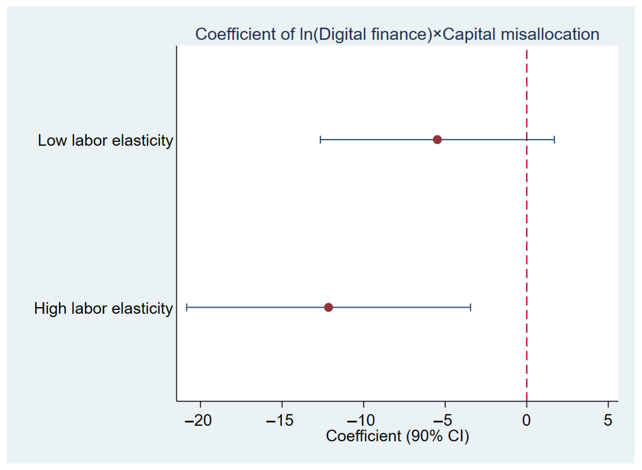
First, labor output elasticity may amplify the adverse impact of capital misallocation. In regions with high labor elasticity, agricultural output is more sensitive to input allocation. Since capital misallocation also influences labor input, the negative effect of digital finance is expected to be stronger in such areas.
Table 6 reports the heterogeneity analysis by labor output elasticity. Cities are divided into two groups: low (below the median) and high (above the median). The results show that the interaction between digital finance and capital misallocation is significantly negative only in regions with high labor output elasticity, indicating that the adverse effect of digital finance on agricultural TFP is concentrated where labor contributes more strongly to agricultural production.
Figure 1 shows the above results.
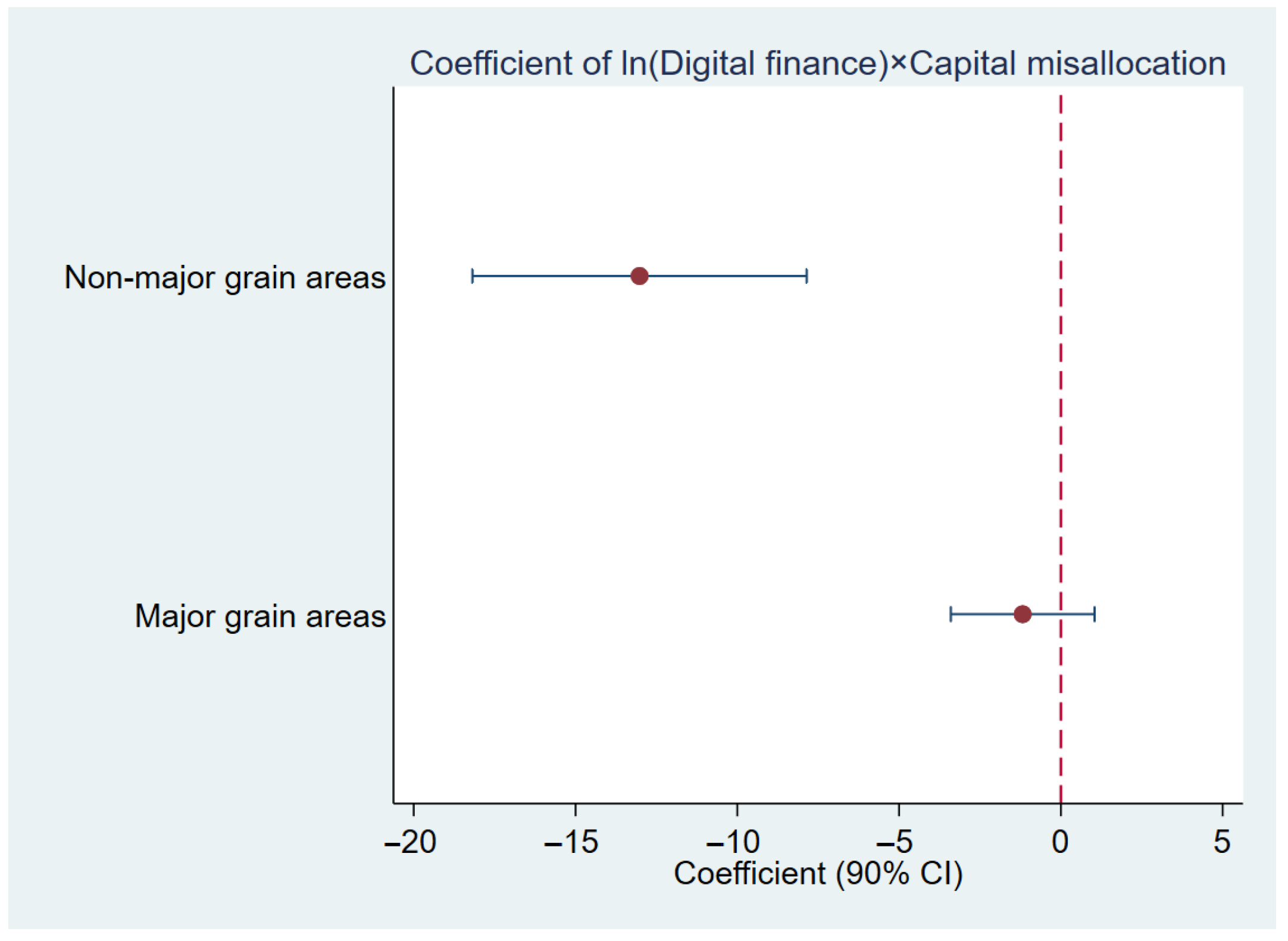
A second dimension of heterogeneity arises from grain production status. Non-major grain-producing areas typically receive weaker financial support and less policy protection, leaving them more vulnerable to capital crowding-out.
Table 7 reports the results for major and non-major grain-producing regions. The coefficient on the interaction term between digital finance and capital misallocation is significantly negative at the 1% level only in non-major grain-producing areas, suggesting that these regions are particularly exposed to the adverse effects of digital finance. By contrast, the interaction effect is insignificant in major grain-producing areas, consistent with the notion that stronger natural resource endowments and policy support buffer the negative impact.
Figure 2 shows these results.
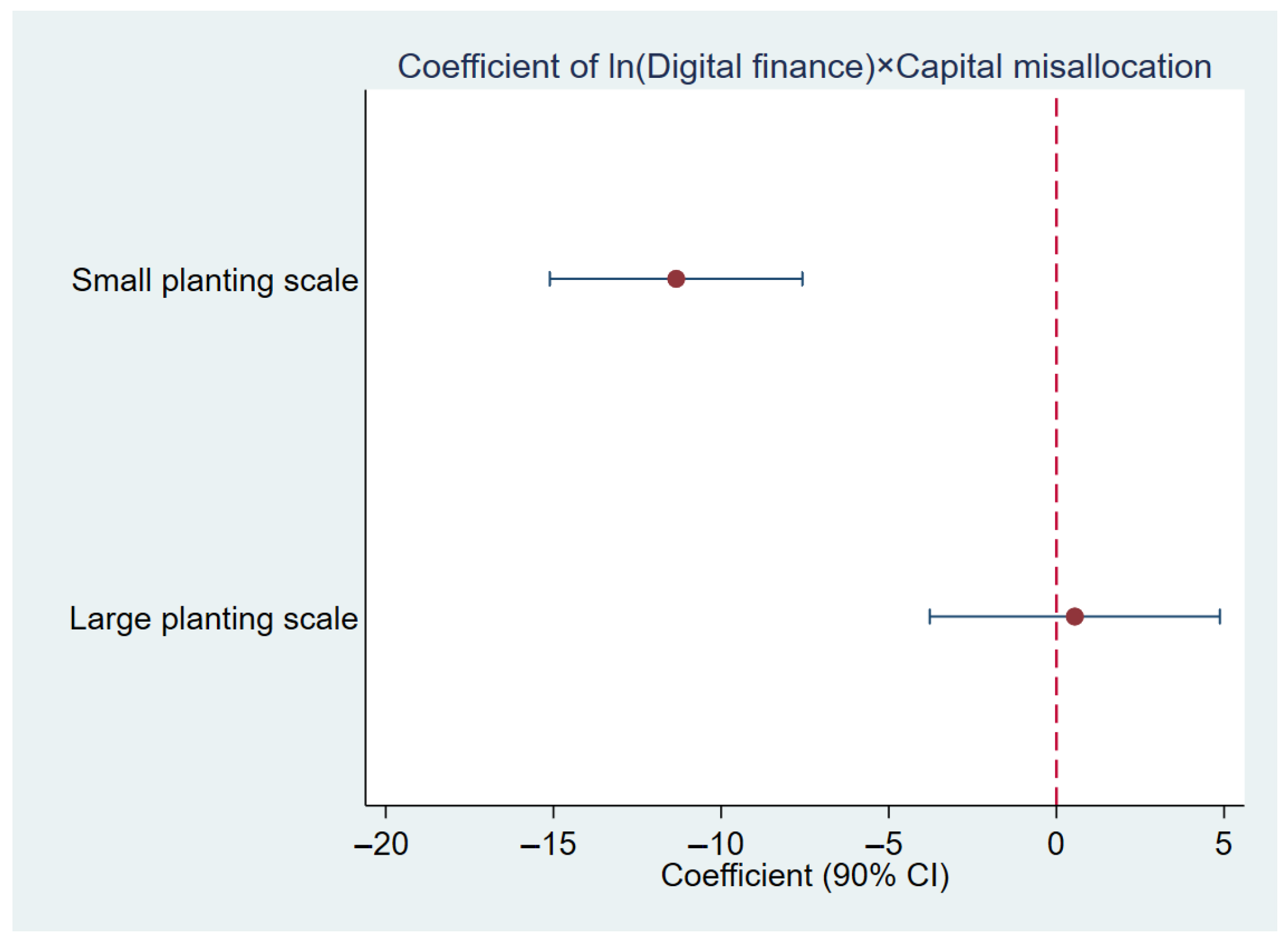
Finally, cultivation scale is another source of heterogeneity in the impact of digital finance on agricultural TFP. Small-scale farms, constrained by limited information and weaker links to formal financial institutions, receive less attention from financial intermediaries and are thus more vulnerable to capital misallocation and crowding-out effects. By contrast, larger-scale farms—better integrated into financial networks and able to demonstrate stable returns—are relatively insulated from such distortions. Columns (1) and (2) of
Table 8 report results based on the median per capita cultivation scale (crop planting area per agricultural worker). The interaction between digital finance and capital misallocation significantly reduces agricultural TFP in small-scale farming regions, whereas the effect is statistically insignificant in large-scale regions.
Figure 3 shows these results.


