Interactive Effects of Relative Land Transport Infrastructure Improvements on Urbanization in China

Abstract

Most studies link transport infrastructure to urbanization using mode-specific stocks or absolute scale, leaving the interactive effects of land transport infrastructure (LTI) and their stage-dependent effects underexplored. To fill this gap, this study examines the interactive effects of relative improvements in LTI on the relationship between urbanization and economic development. Using panel data covering 31 Chinese provinces (2000–2022) and the Gompertz function to model urbanization dynamics and the income elasticities. The modeled urbanization growth rate approaches zero near RMB 600,000 per capita, consistent with a saturation level of 12.2; the peak income elasticity is 1.39 at about RMB 90,000. Results by subsample reveal that high-accessibility roads support early urbanization, while rising incomes see conventional rail, high-mobility roads, and high-speed rail sequentially supporting more sustained urban growth. A mid MPA (balanced high-accessibility and high-mobility roads) fosters more advanced and sustained urbanization, whereas high MPA is detrimental to urbanization. Interaction analysis indicates that prioritizing high-accessibility roads and conventional rail best supports urbanization works at low income; conventional rail and high-mobility roads at mid income; and high-mobility roads and high-speed rail at high income; elasticity patterns mirror these stages. The estimates indicate that a configuration of low RPA and high HPM is linked to lower urbanization. These findings highlight the dynamic and stage-dependent impacts of LTI on urbanization, emphasizing that transport infrastructure strategies should be tailored to different stages of economic development to achieve faster and more sustainable urban growth.

1. Introduction

Urbanization has been recognized as a pivotal driver of socioeconomic development worldwide [1,2,3,4,5,6,7]. In China, rapid economic ascent over the past three decades coincided with unprecedented urbanization: the National Bureau of Statistics (NBS) reports an increase from 26.23% (1990) to 63.89% (2020) alongside a gross domestic product (GDP) of US$14.7 trillion in 2020. This co-evolution has unfolded in parallel with a large expansion of LTI, underscoring the tight linkage between transport development and urban growth.

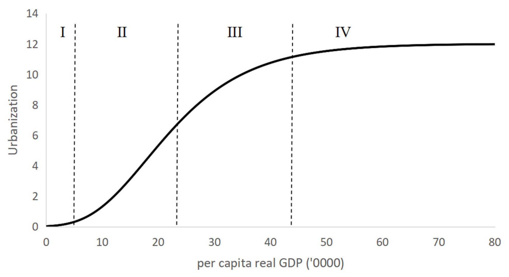
Urbanization typically follows an attenuated S-shape: a gradual take-off, acceleration, deceleration, and stabilization [8]. Understanding this trajectory and its relationship with transport development is crucial for sustainable urban planning and economic policy formulation.

LTI serves as a fundamental catalyst for urbanization through multiple mechanisms. Recent studies document a robust positive association between transport infrastructure and urbanization and related development outcomes [9,10,11]. Efficient LTI facilitates rural-to-urban migration, encourages population concentration, stimulates business growth, and enhances economic activity by improving network connectivity and door-to-door accessibility—particularly where station-area and feeder access are well integrated [6,12]. The World Bank further emphasizes that the influence of LTI on urbanization is a dynamic, multi-dimensional process shaping regional development across economic, social, and spatial domains [13].

LTI in this study comprises railways and roads that vary by mobility and accessibility. Roads with higher accessibility, for example, local roads, can offer more direct routes to specific destinations locally but provide limited mobility. On the other hand, roads with greater mobility, such as highways and major roads, can provide uninterrupted long-distance travel with high speeds between interregional but limited access [14,15]. The conventional railway (CR) system has greater mobility and capacity, lower costs over extended distances, and higher energy and carbon efficiency than roads [16,17]. High-speed rail (HSR) further raises speed, frequency, reliability, comfort, safety, and punctuality, and is generally more energy- and carbon-efficient [18,19]. However, both CR and HSR have limited door-to-door accessibility, so they do not provide direct access to final destinations without feeder connections [19,20,21]; conversely, road effects attenuate with distance [6,16].

Understanding the evolution of transport demand across stages of economic development is crucial for effective infrastructure planning. As urbanization progresses, the type and function of LTI required undergo significant shifts. In the early stages, when population concentration is limited, localized travel dominates, making high-accessibility (HA) roads essential for supporting initial urban growth. With industrialization and the expansion of interregional trade, demand shifts toward CR, which offers greater mobility and capacity, and long-distance transport services. As urban areas expand into suburban zones and economic activities diversify, greater accessibility to commercial services fosters personalized and flexible transport demands, thereby increasing reliance on high-mobility (HM) roads. In the mature stage of urban development, as cities evolve into innovation and economic hubs, high population density brings challenges such as congestion and traffic accidents. These issues drive surging demand for transport systems that are faster, low-latency, high-capacity, frequent, safe, and efficient. HSR thus emerges as the most effective mode to integrate dispersed urban systems, enhance regional connectivity, and mitigate these urban challenges.

From the supply side perspective, areas in the initial stages of urbanization typically exhibit limited economic activity and localized mobility demand, necessitating investments in HA roads to support local travel and facilitate rural-to-urban migration. As industrialization deepens and economic activities diversify, resources must be progressively allocated toward enhancing transport mobility, flexibility, capacity, and efficiency (such as CR and HM roads) to accommodate shifting transport demands, thereby sustaining economic development. At advanced stages, investment in HSR becomes essential to meet the growing demand for premium transport services, enabling the efficient flow of high-end production factors and supporting innovation-driven, sustainable urban growth.

Despite extensive work on transport and urbanization, the literature still seldom evaluates how relative improvements across modes shape the income–urbanization relationship by stage. Recent studies continue to examine single modes—especially HSR—and report economic or environmental effects without jointly modeling the roles of CR and road networks or their portfolio composition (e.g., [11,21,22,23]). Evidence on LTI composition and interaction remains limited: most papers rely on mode-specific stocks or absolute capacity, rather than ratio-based portfolios that capture LTI trade-offs [9,23]. This study addresses that gap by focusing on relative LTI composition and its stage-contingent effects on elasticity peaks and saturation along the urbanization path.

Several mathematical models, including logistic, logarithmic, and Gompertz models, have been employed to simulate and forecast the attenuated S-shaped urbanization curve [24,25,26,27,28]. Previous studies have indicated that historical urbanization data align more accurately with the Gompertz model than alternatives [24,25,28]. Therefore, this study utilizes the Gompertz model to examine how urbanization responds to relative improvements in different LTI types under varying levels of economic development.

Drawing on a provincial panel for 31 Chinese provinces (2000–2022), relative LTI ratios are constructed to track changes in the composition of LTI and to assess how alternative portfolios shape the income–urbanization relationship. This study makes three contributions. Methodologically, a Gompertz–income framework is formalized to read urbanization through Gompertz and income-elasticity curves, and relative LTI portfolios are operationalized to prioritize structural composition over absolute scale. Empirically, a stage-contingent sequence is documented as income rises, showing how advances in rail (HSR and CR) and roads (HM and HA roads) interact to shift elasticity peaks and saturation levels. Theoretically and for policy, a stage-matching principle is articulated for portfolio design—prioritizing HA and CR at low incomes, HM and CR at mid incomes, and HSR and HM at high incomes—thereby reframing planning from “more of everything” to development-stage portfolio optimization.

The rest of the paper is organized as follows. Section 2 reviews factors associated with urbanization, organizing recent evidence on income, demographics, institutions, and land-transport supply/composition. Section 3 presents the theoretical framework organized around four mechanisms. Section 4 describes data sources and variable construction. Section 5 details the methodology, including the Gompertz specification, elasticity derivation, and grouping logic. Section 6 reports results and discussion—baseline estimates, interaction analyses, mechanism-based interpretation, and policy-relevant synthesis. Section 7 concludes with contributions, stage-matched policy guidance aligned to national strategies, limitations, and directions for future research.

2. Factors Associated with Urbanization

Demand for urban living rises with economic activity and standards of living, making urbanization closely associated with income. Higher incomes reduce migration and settlement frictions, increasing the propensity to move to cities and to afford housing, transport, and public services [1,13,18,29]. In predominantly agrarian contexts, limited non-agricultural opportunities and constrained urban service capacity are linked to persistently low urbanization [30,31,32].

While per capita GDP is a strong predictor of urbanization, it does not fully explain the differences in urban growth patterns among countries or regions with similar income levels. Variations in accessibility and transport quality, demographic structure, institutions, and spatial form shape both the velocity and saturation of urbanization [9,16]. Recent work emphasizes that accessibility and urban form—through their environmental performance and livability effects—help explain cross-place differences in saturation levels [6,7,33,34].

Extensive empirical evidence demonstrates marked heterogeneity in urbanization growth patterns—both in terms of velocity and saturation levels—between developed and developing regions [35,36,37,38]. As incomes rise, the pace and saturation level of urbanization in developing countries are expected to increase substantially compared with developed countries [13]. In China, for instance, the urbanization rate surged from 26.23% in 1990 to 63.89% in 2020, a pace described as “much faster than the increase observed in other income groups and the average speed worldwide” [36,37,39,40,41]. In contrast, many developed countries experience a slowdown or even counter-urbanization because of urban diseconomies such as congestion, pollution, rising housing costs, and declining quality of life in metropolitan areas [42,43]. Similar patterns have been documented recently in Germany, Sweden, and the UK [44,45,46]. Evidence on induced travel further suggests that added road capacity attenuates long-run congestion relief, limiting the payoff from single-mode expansion in advanced urban systems [13,47]. These findings suggest that while income level is strongly related to urbanization growth, it is insufficient alone to compare urbanization demand across countries at varying stages of economic development.

Regional disparities in the quantity and quality of LTI constitute a critical determinant of asynchronous urbanization patterns across regions. These disparities reflect transformative shifts in the scale of economic activity and the demand for mobility and accessibility as development proceeds [9,16]. As regions grow, road and rail networks expand to meet rising demand—especially for long-distance, high-capacity, and efficient movement of people and goods—so where and how the LTI improves matters for welfare and urbanization outcomes [16,48]. Reliance on higher-quality LTI becomes increasingly pivotal as urban footprints spread and activities decentralize, elevating the need for robust intercity links and well-connected feeders [6,18,49,50]. Empirically, improvements in quality, coverage, and accessibility of LTI—rather than mileage alone—are associated with higher urbanization levels and more inclusive gains [16,51]. Conversely, highly urbanized regions may face deceleration as transport-related externalities intensify [50,52]; evidence on induced travel and the cost-of-living/housing squeeze indicates that capacity-led expansion can have limited congestion relief and exacerbate urban diseconomies [34,47].

Taken together, these patterns motivate a stage-contingent theory of how relative LTI composition—across HSR, CR, HM, and HA—reallocates accessibility, mobility, and capacity to shape the income–urbanization curve. The next section develops this theoretical framework.

3. Theoretical Framework

Urbanization and income are tightly correlated and typically follow an attenuated S-shaped trajectory with take-off, acceleration, deceleration, and stabilization [8,38,53]. Drawing on transport–development theory, the income–urbanization linkage can be organized into four stage-dependent mechanisms operating through the relative composition of LTI: (M1) the size of economic activity, (M2) the migration transition effect, (M3) the transport demand evolution effect, and (M4) the service quality optimization effect [9,16,48,50,54,55].

The size of economic activity is a result of income growth; however, at low income, economic activity is thin and spatially local, leading to the basic accessibility and essential transport demand. HA roads reduce first/last-mile frictions, connect rural areas to towns, and support initial market integration; urbanization responds, but elasticity remains modest (corresponds to Zone I of Figure 1) because activity and capacities are limited [48].

As incomes reach middle levels, advances in industrialization expand non-agricultural employment, followed by large-scale rural-to-urban migration. Demand needs to shift toward long-distance, high-capacity flows, with CR functioning as the workhorse—offering mobility, capacity, and safety that raise efficiency and enable cities to absorb surplus rural labor, thereby accelerating urbanization [31,36,55]. The migration transition effect causes urbanization to rise sharply as income increases, corresponding to Zone II in Figure 1.

With further income growth, trips become more frequent, longer, and more spatially dispersed across metropolitan regions. HM roads—expressways and major arterials—provide flexible, time-reliable connectivity for commuting and inter-urban business travel, reinforcing polycentric patterns. Urbanization continues to rise, although the elasticity moderates as network externalities emerge [35,55]. The transport demand evolution effect keeps urbanization growing, but at a moderating pace, corresponding to Zone III in Figure 1.

The service quality optimization effect emerges at the high-income stage when urbanization approaches saturation, accompanied by negative externalities such as traffic congestion, increasing road accidents, and environmental degradation [42,56]. Higher incomes create greater elasticity of demand for premium transport services—those that are time-sensitive, high-capacity, and safer—which help alleviate these issues and encourage a modal shift from private cars to HSR [43,50]. As a result, even as income continues to grow, urbanization stabilizes near its saturation level, corresponding to Zone IV in Figure 1.

4. Data Sources and Variables

This section delineates data sources and the variables employed in this study.

Table 1. Variables definition and data source.

Variables	Definition	Data Source
GDP	Per capita real gross domestic product	National Bureau of Statistics (NBS)
URB	Ratio of urban population to rural population
HPR	Ratio of the total mileage of HSR to the total mileage of CR
HPM	Ratio of the total mileage of HSR to the total mileage of HM roads
HPA	Ratio of the total mileage of HSR to the total mileage of HA roads
RPM	Ratio of the total mileage of CR to the total mileage of HM roads
RPA	Ratio of the total mileage of CR to the total mileage of HA roads
MPA	Ratio of the total mileage of HM roads to the total mileage of HA roads

presents a comprehensive overview of the data incorporated in this study, along with their respective sources and definitions. The analysis is based on panel data, encompassing 713 annual observations for 31 provinces in China spanning from 2000 to 2022, as shown in Table S1.

Urbanization (URB), the dependent variable, is measured as the ratio of urban population to rural population. The independent variable is economic development, measured by per capita real GDP. It is calculated at constant prices using regional GDP deflators, thereby effectively mitigating the influence of price fluctuations over time.

The LTI ratio variable was derived by comparing the cumulative lengths of HSR, CR, HM, and HA roads. For instance, HPR is calculated by dividing the cumulative length of HSR by that of CR, and MPA is derived from the ratio of HM road mileage to HA road mileage. As defined by the National Railway Administration, HSR lines are those with an average operational speed of no less than 250 km/h (or intercity passenger-dedicated lines with speeds no less than 200 km/h), while CR lines refer to conventional railways operating below 140 km/h.

For roads, the International Road Federation (IRF) classifies expressways and national highways as HM roads, while secondary, regional, and other roads fall under HA roads. In China’s NBS road accounts, mileage is reported in five technical classes: expressways, Class I, Class II, Class III, and Class IV. To ensure cross-provincial and intertemporal comparability, and align with the IRF functional typology, we assign expressways and Class I to HM roads, and Class II–IV to HA roads.

This study measures land-transport development using scale-free mileage ratios (e.g., MPA) to capture the relative composition of the LTI rather than its absolute size. This choice aligns with the paper’s stage-matching question—which portfolio mix matters at which income stage—and enhances cross-provincial comparability by attenuating differences in area, population, and fiscal capacity. It also relies on the most consistently reported provincial series over 2000–2022. By construction, these ratios proxy spatial reach and portfolio balance and are less sensitive to common growth in totals [9,16]. In contrast, operational attributes of LTI (connectivity, frequency, and efficiency) are inherently model-dependent and definition-sensitive, leading to different observations, and the NBS does not maintain uniform statistical standards for these indicators. Moreover, in our framework, these indicators are mechanisms through which structural LTI portfolios translate into outcomes. Mileage-based ratios compiled under national accounting rules therefore offer a scale-free, auditable, and comparable proxy of structural composition and spatial reach. Accordingly, results are interpreted as portfolio-composition effects, not short-run operational performance.

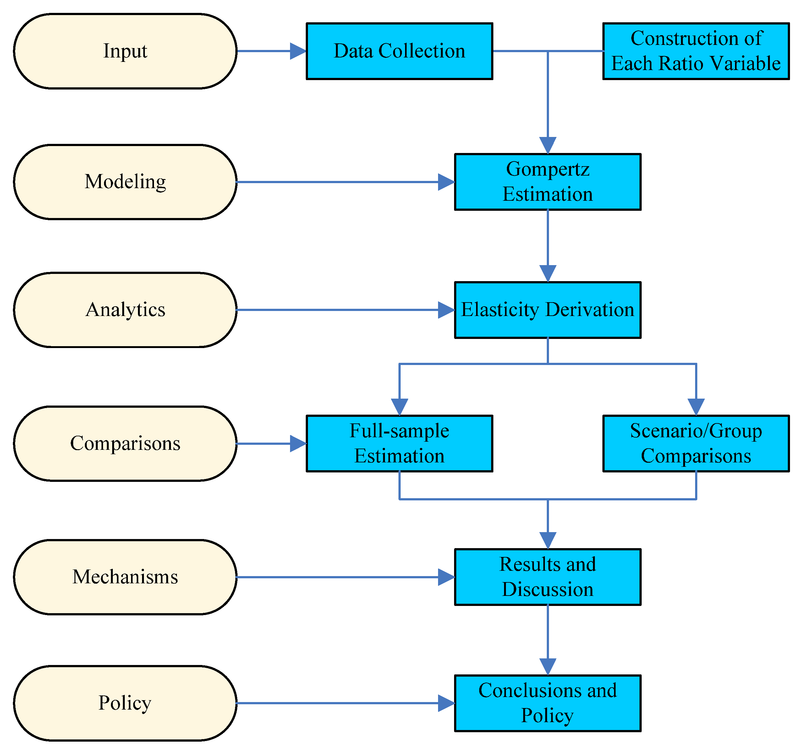
Figure 2 summarizes the overall workflow—from data harmonization and construction of relative LTI ratios to Gompertz estimation, elasticity derivation, full-sample estimation, scenario/group comparisons, discussion, conclusions, and policy.

5. Methodology

Following the workflow summarized in Figure 2, we proceed from ratio construction to Gompertz estimation, elasticity derivation, and scenario/group comparisons, discussion, conclusions, and policy. This study employs the Gompertz nonlinear least squares regression model to investigate the complex relationship between LTI development, economic growth, and urbanization patterns. The Gompertz model has been widely recognized for its efficacy in capturing nonlinear relationships in transportation and urban development contexts [57,58]. Economic performance measured by per capita real GDP serves as the independent variable, while the level of urbanization—measured as the ratio of urban to rural population—is treated as the dependent variable. Following the theoretical framework of Henderson [59], urbanization follows a nonlinear S-shaped trajectory. This relationship can be formulated as follows:

$$U_{it}=\gamma e^{\alpha \mathrm{e}\mathrm{x}\mathrm{p}\left(\beta y_{it}\right)}$$

(1)

where U represents urbanization, y_it denotes economic performance, i indicates province, t represents year, $\gamma$ signifies the saturation level of urbanization, while α and β are parameters that determine the shape of the growth curve. The parameter α controls the curve’s position along the income axis. A larger α moves the entire S-curve horizontally to the right, so that for the same level of economic performance, the predicted urbanization level is lower. Economically, a higher α indicates that the take-off and acceleration phases occur at higher income levels (see Figure 3: the orange curve is shifted right relative to the blue curve). The parameter β governs the rate at which urbanization rises from take-off toward the saturation level. A larger β yields a steeper slope around the inflection region and faster convergence to saturation—that is, the system reaches its ceiling sooner in income space (see Figure 4: the blue curve approaches the plateau more quickly than the orange curve).

This study further employs the income elasticity curve to delineate the evolving pattern of the Gompertz curve and its implications for urbanization across income levels. The income elasticity curve, derived from the Gompertz function, manifests a bell-shaped form with varying skewness and peak values (Figure 5). Curves with greater positive skewness reflect steeper elastic slopes before reaching the peak—for instance, the black curve exhibits a sharper incline than the red curve before both attain the same saturation level. This suggests that Gompertz curves with steeper elasticity profiles lead to faster urbanization growth before saturation.

The income threshold corresponding to the saturation point of the urbanization Gompertz curve coincides with the income level at which the elasticity curve falls to zero. A decline to zero at higher income levels indicates greater potential for sustained urban growth, whereas an earlier decline suggests limited urbanization prospects. As illustrated in Figure 5, the green elasticity curve declines to zero at a higher per capita GDP than the purple curve. This implies that although the purple curve exhibits a higher peak elasticity, its urbanization process saturates earlier, while the green curve supports a more sustainable growth. Such comparison is employed to analyze how relative improvements in various LTI types interactively influence the dynamics and sustainability of urbanization.

Equation (1) was differentiated to derive the income elasticity of urbanization growth, expressed as follows:

$$I=\alpha \beta \gamma e^{\beta \gamma }$$

(2)

$$r_M={\displaystyle \frac{-1}{\beta }}$$

(3)

$$I_M=-0.3678\alpha$$

(4)

where I represents income elasticity of urbanization; r_M represents income level at the maximum income elasticity, marking the income turning point on the S-curve where urbanization shifts from acceleration to deceleration; and I_M is maximum income elasticity, indicating how responsive urbanization is at its most sensitive stage and, by implication, the marginal payoff to income growth at the peak.

Equation (1) was modeled to examine the effects of distinct LTI ratio variables on the relationship between economic performance and urbanization, while the effects of income elasticity on urbanization were tested using Equation (2).

To examine the heterogeneous impacts of LTI configurations on urbanization, the sample is divided into subgroups based on threshold values of key transport ratio indicators. The grouping threshold is set around the 60th percentile to better capture the dominance of one LTI type over another, thereby facilitating the detection of nonlinear effects on urbanization and aligning with the view that only dominant infrastructure exerts significant influence on urban development patterns [35,60]. Particularly, the variable MPA was divided into low, mid, and high MPA groups based on two cutoff points, and the sample size ratio is 40:40:20. Furthermore, to explore more complex interactive effects of LTI, the study adopts a hierarchical grouping approach, aligning with emerging methodologies in regional development and transport economics that emphasize the heterogeneity of infrastructure effects [60,61,62]. The exact numerical thresholds for each ratio variable used in the study are shown in

Table 2. Cut-off points for each ratio variable.

Variable	Cut-off Point 1	Cut-off Point 2
RPA	0.055	-
RPM	0.1751	-
HPA	0.035	-
HPM	0.0285	-
MPA	0.378	0.676

.

6. Results and Discussions

Table 3. Descriptive statistics for all variables.

Variable	Observation	Average	Standard Deviation	Minimum	Maximum
GDP	713	3.855	3.131	0.276	19.000
URB	713	1.523	1.520	0.240	8.375
HPR	713	0.479	0.699	0.000	4.081
HPM	713	0.026	0.046	0.000	0.863
HPA	713	0.041	0.060	0.000	0.384
RPM	713	0.240	0.173	0.000	1.600
RPA	713	0.102	0.074	0.000	0.686
MPA	713	0.528	0.476	0.000	4.666

provides the descriptive statistics for each variable. Meanwhile, Model A in

Table 4. Estimated parameters of urbanization models for overall sample, by RPA level, by interaction between RPA and HPM level.

	Gompertz	RPA		Low RPA		High RPA
		Model B1	Model B2	Model C1	Model C2	Model C3	Model C4
Estimated Parameters	Model A	Low RPA	High RPA	Low HPM	High HPM	Low HPM	High HPM
γ	12.19935 *** (1.998778)	9.986012 ** (2.029461)	12.93568 *** (2.914425)	9.385014 *** (0.8472402)	3.589676 *** (0.8623463)	8.11634 *** (1.45738)	11.32411 *** (2.20085)
α	3.789562 *** (0.1362866)	3.653423 *** (0.4020537)	3.698088 *** (0.1677308)	4.025711 *** (0.4712403)	1.591316 *** (0.2552375)	4.055648 *** (0.26952)	3.865648 *** (0.1724482)
β	0.1106462 *** (0.0130561)	0.147735 *** (0.0300235)	0.0962162 *** (0.0138212)	0.2014079 *** (0.02898)	0.1489919 ** (0.07366440)	0.1811933 *** (0.0292972)	0.1080502 *** (0.0176587)
Max elasticity	1.39	1.34	1.36	1.48	0.59	1.49	1.42
GDP at max elasticity (‘0000) (RMB)	9.0	6.8	10.4	5.0	6.7	5.5	9.4

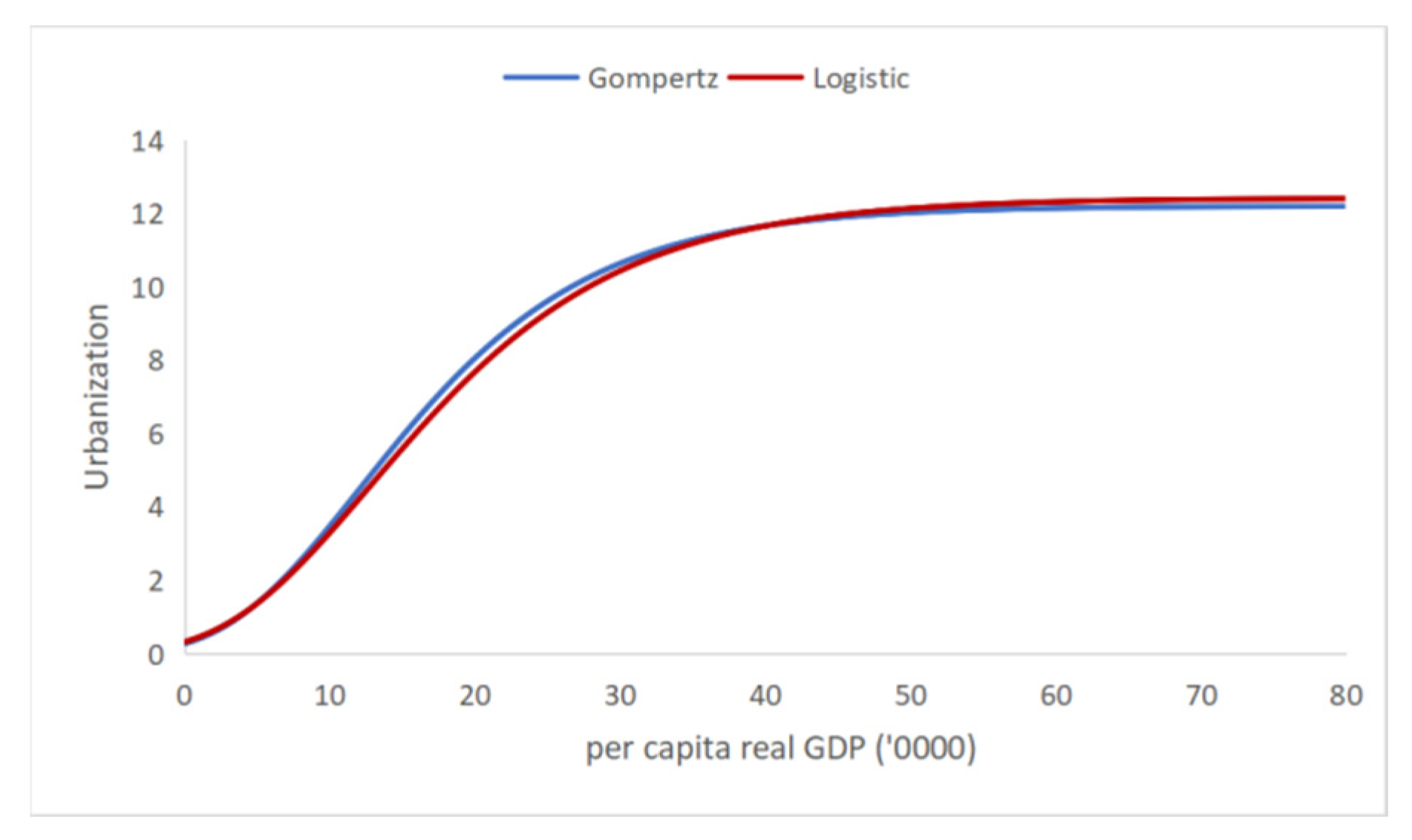
The symbols *** and ** represent statistical significance levels of 1% and 5%, respectively.

presents the results of the Gompertz model for the data from 2000 to 2022, covering 31 provinces in China, illustrating the relationship between urbanization and economic performance. The urbanization growth curve depicted in Figure 6, aligns with classical urbanization theories [8,28]. This S-shaped curve represents the typical trajectory of urbanization across development stages. Alongside the Gompertz model, a standard logistic specification (red curve) is estimated. As Figure 6 shows, the fitted paths are virtually indistinguishable. The Gompertz model is retained as the baseline given consistently lower AIC and BIC (Table S2), and the logistic estimates are reported as a robustness check.

During the initial development phase, inadequate infrastructure and limited employment opportunities result in exceedingly slow urbanization progression. These barriers to rural-urban migration inhibit population mobility [63], thereby maintaining the urbanization rate at relatively low levels. As early industrialization commences and economic activities expand, the rapid growth phase begins, characterized by a markedly accelerated pace of urbanization [36]. Urban areas, offering superior infrastructure, enhanced healthcare services, and more abundant employment opportunities with higher wage premiums, facilitate the swift rural-urban population transition [64]. However, as cities become more developed, urbanization enters a deceleration and saturation phase. During this stage, urbanization velocity gradually diminishes and approaches an asymptotic ceiling as issues such as congestion, pollution, and environmental degradation become increasingly pronounced [65,66,67].

This model A demonstrates that the urbanization growth rate approaches zero when per capita GDP reaches 600,000 RMB, corresponding to the saturation point of 12.20, exhibiting an overall S-shaped curve. The corresponding urbanization elasticity curve presents a steep ascent at lower GDP levels, followed by a gradual decline after reaching its peak, forming an asymmetric normal distribution as illustrated in Figure 7. The elasticity curve reveals that urbanization responsiveness to GDP progressively strengthens until per capita GDP reaches 90,000 RMB, beyond which this responsiveness gradually weakens. This responsiveness indicates that once income reaches a certain threshold, urbanization becomes less elastic, as multiple other factors begin to influence its growth, leading to a slower rate of increase [42,56]. The extent of these effects varies across regions but is typically linked to socioeconomic conditions such as transport infrastructure, technological advancement, and industrial structure [52]. In other words, both income elasticity and saturation levels are dynamic and may shift with changes in these contextual factors. This study examines the impacts of different combinations of LTI to explain variations in urban growth patterns. The estimates of these models are presented in Table 4,

Table 5. Estimated parameters of urbanization models by RPM level and interaction between RPM and HPA level.

	RPM		Low HPA		High HPA
	Model D1	Model D2	Model E1	Model E2	Model E3	Model E4
Estimated Parameters	Low RPM	High RPM	Low RPM	High RPM	Low RPM	High RPM
γ	12.90508 *** (3.819947)	11.66422 *** (2.359656)	7.565189 *** (0.4046678)	9.858694 ** (4.795298)	16.28697 * (9.134659)	13.66375 ** (6.904697)
α	3.898749 *** (0.2813913)	4.047578 *** (0.1550445)	16.75258 *** (6.221013)	3.954007 *** (0.3524559)	3.823782 *** (0.3517322)	4.476876 *** (0.2660558)
β	0.1058406 *** (0.0241416)	0.138577 *** (0.0190131)	0.5036408 *** (0.073828)	0.1778479 *** (0.0491765)	0.0795382 * (0.0278367)	0.1262533 ** (0.0407869)
Max elasticity	1.43	1.49	6.16	1.43	1.41	1.65
RGDP at max elasticity (‘0000) (RMB)	9.4	7.2	2.0	5.6	12.6	7.9

The symbols ***, **, and * represent statistical significance levels of 1%, 5%, and 10%, respectively.

and

Table 6. Estimated parameters of urbanization by low, mid, and high MPA conditions.

	Model F1	Model F2	Model F3
Estimated Parameters	Low MPA	Mid MPA	High MPA
γ	8.577522 *** (0.2942143)	12.14033 *** (3.836104)	5.714699 * (2.073532)
α	5.878759 *** (0.4573954)	3.659212 *** (0.2289685)	3.428936 *** (0.423203)
β	0.327219 *** (0.0221178)	0.1013147 *** (0.0237451)	0.1605432 ** (0.0595966)
Max elasticity	2.16	1.34	1.26
GDP at max elasticity (‘0000) (RMB)	3.1	9.9	6.2

The symbols ***, **, and * represent statistical significance levels of 1%, 5%, and 10%, respectively.

; full goodness-of-fit metrics (AIC, BIC, RMSE) and 95% confidence intervals for γ, α, and β are provided in Tables S3–S5. Residual diagnostics, including residuals versus fitted, normal distribution plot of residuals, and normal Quantile-Quantile plot in Figures S1–S3, show patternless, mean-zero residuals and approximate normality, which supports the adequacy of the Gompertz specification.

6.1. The Interactive Effects of Relative Improvements in RPA and HPM on Urbanization Patterns

6.1.1. The Impact of Relative Improvements in RPA on Urbanization Patterns

The study first examined how relative improvements in RPA influence urbanization patterns, and Models B1 and B2 in Table 4 present the results for low and high RPA conditions, respectively. As illustrated in Figure 8, at lower income levels, regions with lower RPA values generally exhibited higher urbanization levels, consistent with M1. This can be attributed to the fact that in the early stages of development, populations typically concentrate in smaller-scale areas, with economic activities primarily occurring within localized regions, aligning with findings from Ng, Law [14], and Duranton, Morrow [68]. In early development phases, the broad coverage of HA roads, enabling surplus rural labor migration to urban areas, was more critical than transport efficiency.

However, as income increased, a distinct trend emerged whereby high RPA conditions corresponded with higher urbanization levels and an elevated saturation point, matching M2. This phenomenon is closely associated with the expansion of economic activities in both scale and scope, as emphasized by several studies [69,70,71,72]. As incomes reach middle levels, industrialization expands non-agricultural employment, driving rapid growth in demand for long-distance, high-volume transport [69,73]. Therefore, more investments in CR systems—characterized by high capacity, long-distance capability, and greater mobility—rather than HA roads, become essential to meet the rising medium- and long-distance transport demands of industrialization.

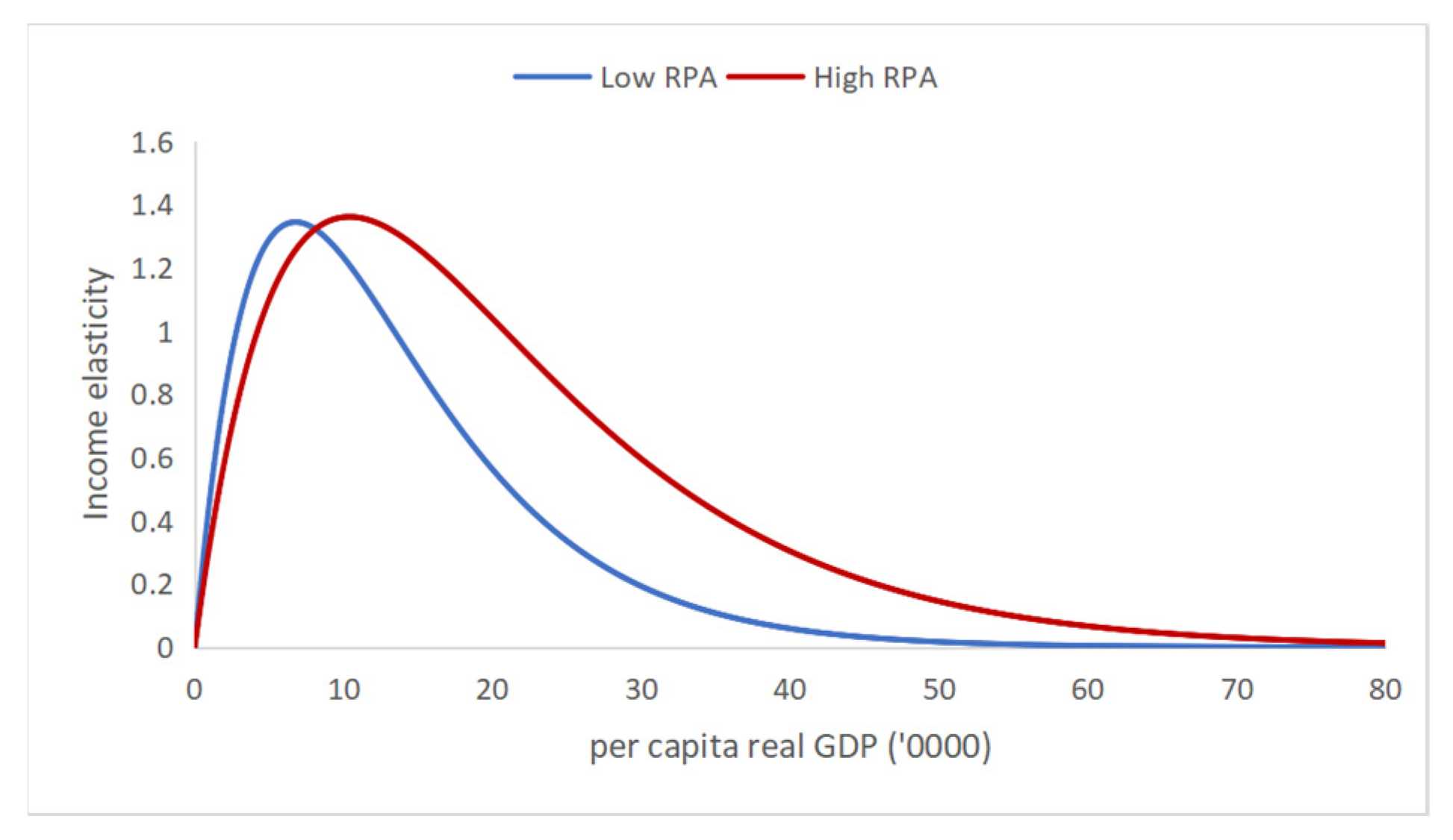
Figure 9 clearly illustrates and compares income elasticity curves under different RPA conditions. Both curves exhibit similar peak values. Before reaching their respective peaks, the elasticity coefficients under low RPA conditions were slightly higher than those under high RPA conditions. However, after peaking, income elasticity under low RPA conditions declined more rapidly compared to high RPA conditions. Furthermore, the per capita GDP at which income elasticity approached zero under low RPA conditions was significantly lower than under high RPA conditions. This suggests that at lower income levels, the accessibility needs of roads outweighed those of CR, primarily benefiting local regional economies and consequently driving urbanization in these areas. Nevertheless, as income gradually increased, the demand for CR transport increased significantly to expand the scale and scope of economic activities.

6.1.2. The Interactive Effects of HPM and Low RPA Conditions on Urbanization Patterns

To further validate the effects of the remaining two types of LTI on the urbanization growth curve, HPM was subdivided into high and low groups based on the RPA classification. Models C1 and C2 in Table 4 demonstrate the estimates of high and low HPM under low RPA conditions on the relationship between economic performance and urbanization. Figure 10 reveals a counterintuitive pattern: urbanization levels under low HPM conditions consistently exceed those under high HPM conditions. 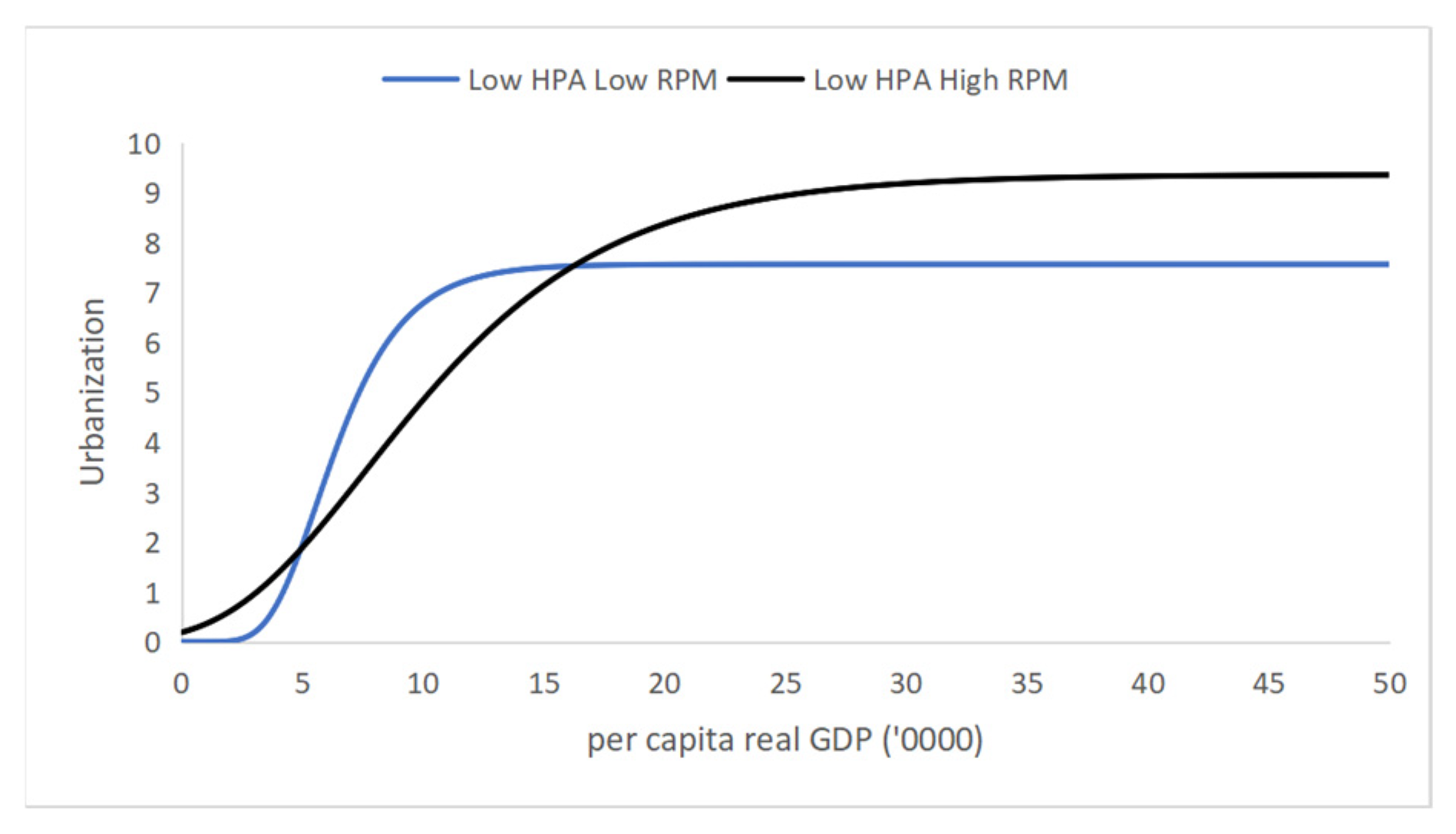This phenomenon highlights the critical role of complementarity and stage-specific utility of LTI in shaping urbanization processes [74].

Under low RPA, low HPM outperforms high HPM as evidence of portfolio mismatch and missing-middle capacity. First, when CR and HM capacity is weak, the first/last-mile and middle-mile links that translate HSR’s line-haul speed into door-to-door accessibility are missing, thereby blunting HSR’s service-quality gains (M4). Recent studies show that station-area accessibility is pivotal for realized HSR mobility and that HSR-related new towns perform heterogeneously unless they are well integrated into local networks [12,43,75,76]. Second, HSR tends to substitute CR in passenger markets while complementing highways. In provinces where CR is already thin, this substitution tightens the bottleneck, further weakening the migration-transition mechanism (M2) and entrenching a strong-trunk/weak-feeder hierarchy [18]. Third, while an HSR-dominant mix improves line-haul speed, it cannot translate those gains into effective door-to-door access when CR feeders and HM links are insufficient. This short-circuiting of the transport-demand evolution pathway (M3) keeps settlement frictions high and constrains the transition from short-term mobility to stable urban residency [77]. Finally, early prioritization of HSR can crowd out needed upgrades to CR and HM, undermining the migration-transition and transport-demand evolution mechanisms (M2 and M3). This leaves meso-scale passenger/freight flows underserved and reduces agglomeration benefits, and is associated with environmental externalities that erode the quality of urbanization [78,79].

In contrast, under low RPA and low HPM, it is preferable to emphasize HM construction rather than HSR (M3). Together with CR and well-developed HA, this portfolio creates a complementary LTI network that provides fundamental regional connectivity and flexibility. This balanced transport supply structure is crucial for effectively matching multi-level travel demands within regions [50,80] and supporting middle-stage industrialization and regional integration development [81,82]. HSR’s M4 benefits, such as knowledge spillovers, can only be realized after urban agglomerations mature [52].

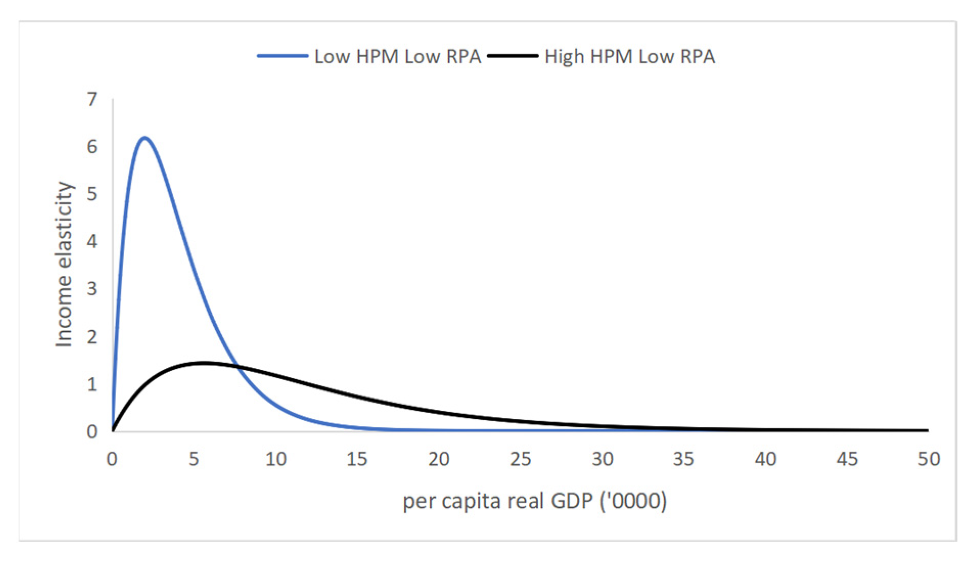
In Figure 11, the peak value of the blue income elasticity curve not only far exceeds that of the black curve, but the former elasticity curve consistently exceeds the latter. This result indicates that under low RPA conditions, demand for HM roads far outweighs demand for HSR.

6.1.3. The Interactive Effects of HPM and High RPA Conditions on Urbanization Patterns

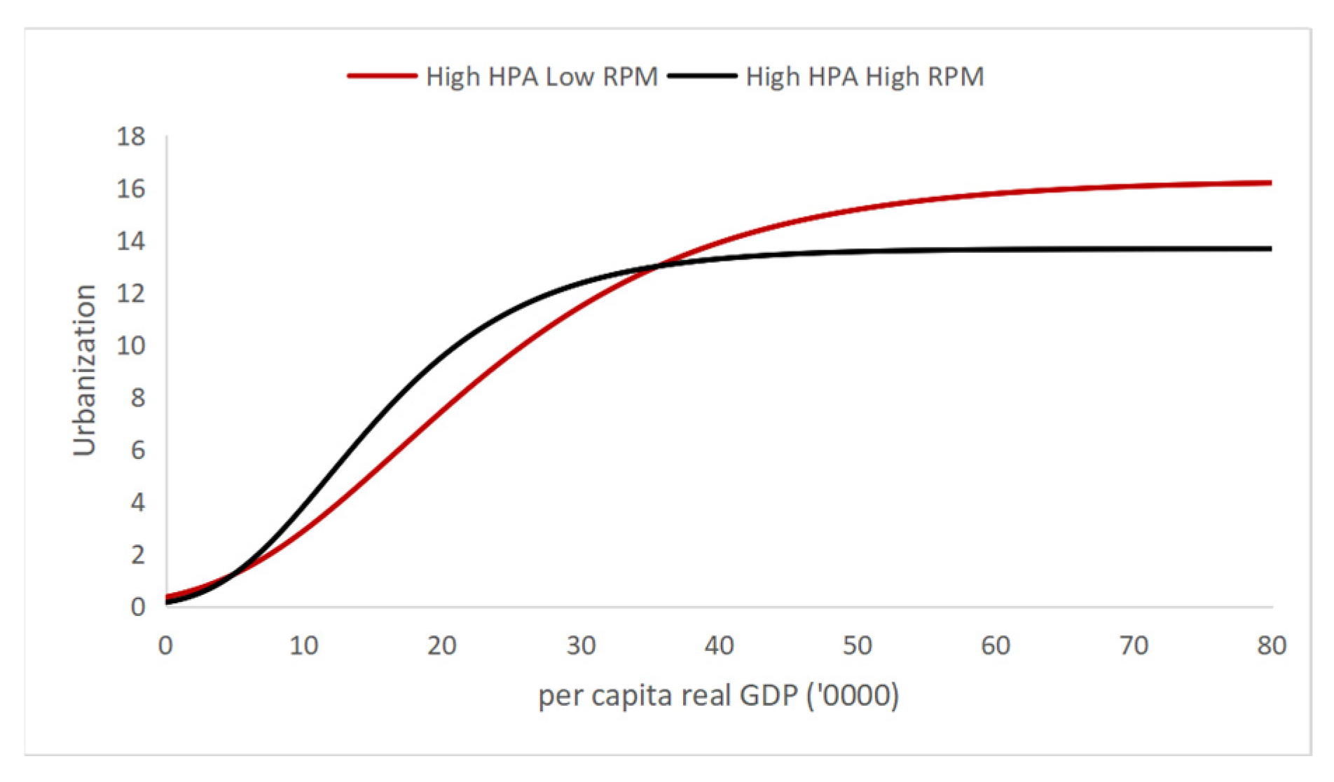
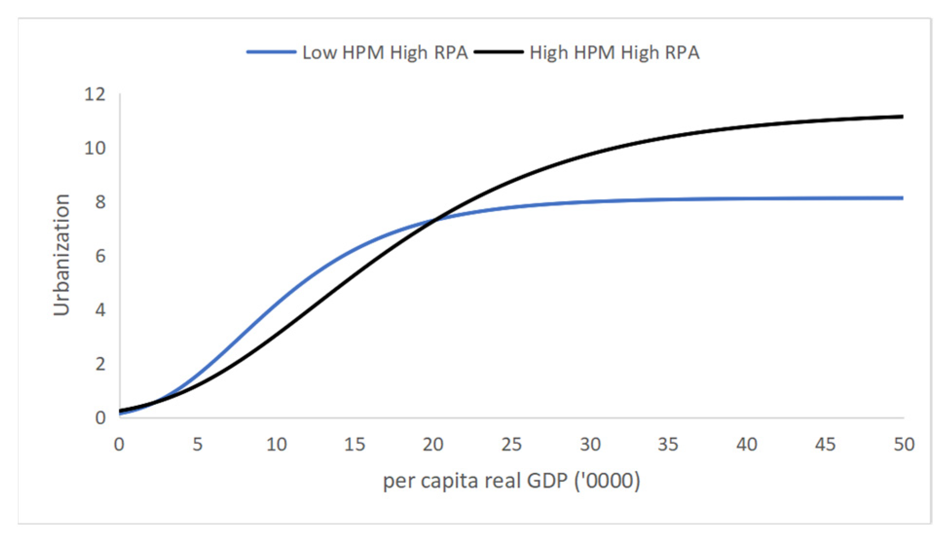
Models C3 and C4 in Table 4 illustrate how high and low HPM affect the relationship of economic performance and urbanization under high RPA conditions. The Gompertz curves under high RPA conditions with high and low HPM in Figure 12 resemble those of RPA. Under high RPA conditions, low HPM conditions typically correspond with higher urbanization levels compared to high HPM conditions at mid-income levels. This finding suggests that during mid-income stages, a configuration characterized by a greater emphasis on HM roads combined with CR is more effective (aligned with M2 and M3) in promoting urbanization than one that relies more heavily on HSR with CR. This result is supported by previous studies, which suggest that enhancing CR and HM roads can more effectively accommodate industrialization-driven structural transformation and evolving transport demand, respectively [50,83].

However, at higher income levels, urbanization levels under high HPM conditions gradually exceed those under low HPM conditions and exhibit higher saturation points. This result indicates that at this stage, a configuration featuring a greater emphasis on HSR combined with CR is more effective in promoting urbanization compared to the other (corresponding to M4). This implies that as urbanization approaches saturation with rising income, transport demand becomes increasingly sensitive to efficiency and time costs, leading to a surge in the need for premium transport services [52,84]. At this stage, a configuration with greater HSR together with CR (M2 combined with M4), rather than lower HSR, is more effective in alleviating congestion and other negative externalities associated with high urbanization [43,50]. This is because HSR provides transport service-quality optimization (M4) characterized by higher efficiency, larger capacity, greater safety, and lower delays, which cannot be matched by other LTI, thereby advancing urbanization to higher levels [71].

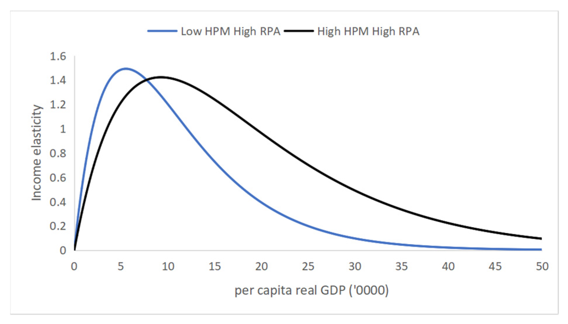
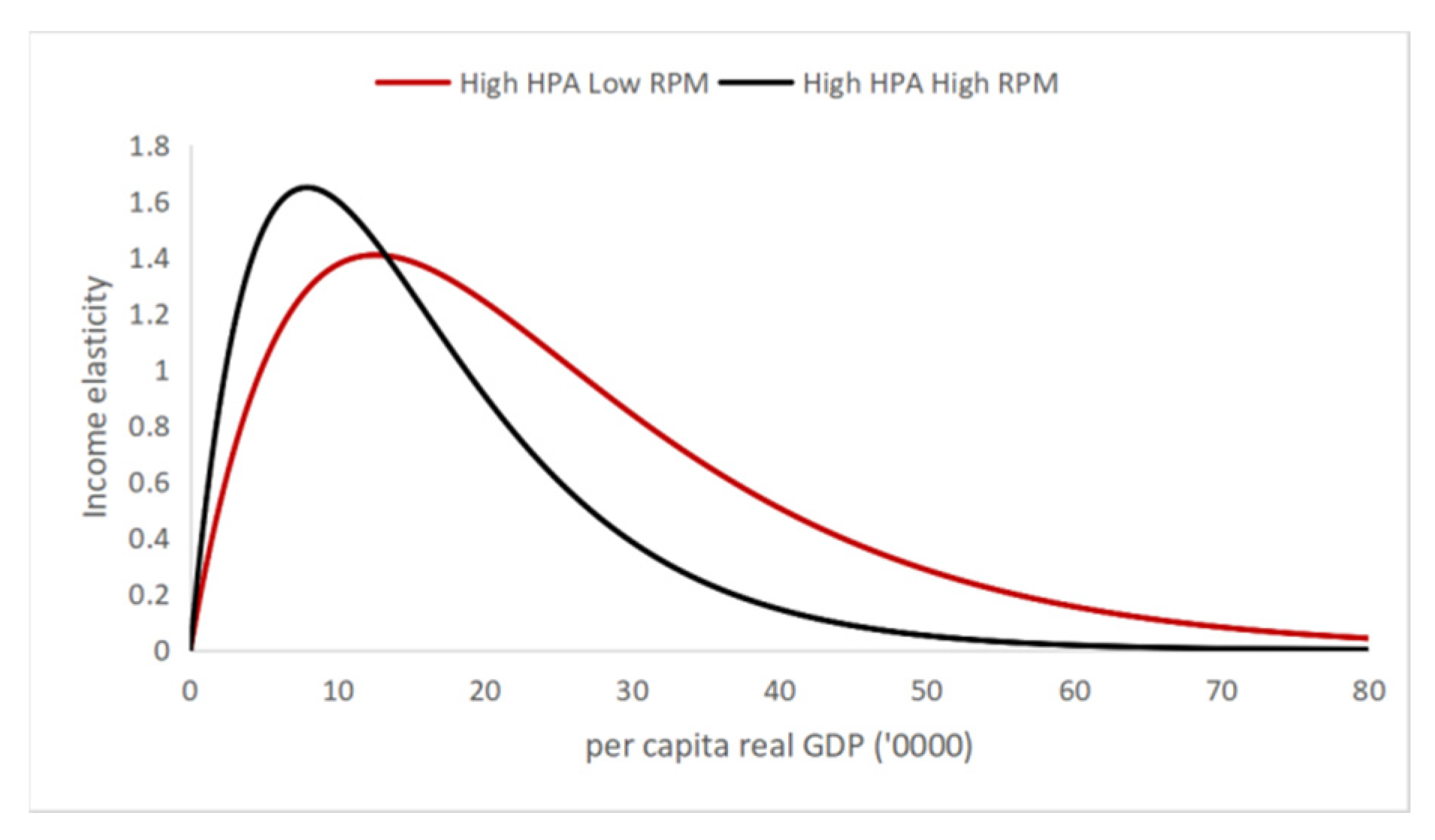
Figure 13 presents income elasticity curves for high and low HPM under high RPA conditions. These curves exhibit similar peak values, with low HPM elasticity coefficients slightly exceeding high HPM coefficients before the blue curve reaches its peak. However, after the blue curve exceeds its peak, income elasticity declines more rapidly. This result suggests that under high RPA conditions, the urban growth pattern supported by high HPM has greater potential to push urbanization toward higher levels compared to low HPM, confirming HSR’s importance in advancing urbanization processes toward higher levels at higher GDP levels.

6.2. The Interactive Effects of Relative Improvements in RPM and HPA on Urbanization Patterns

6.2.1. The Impact of Relative Improvements in RPM on Urbanization Patterns

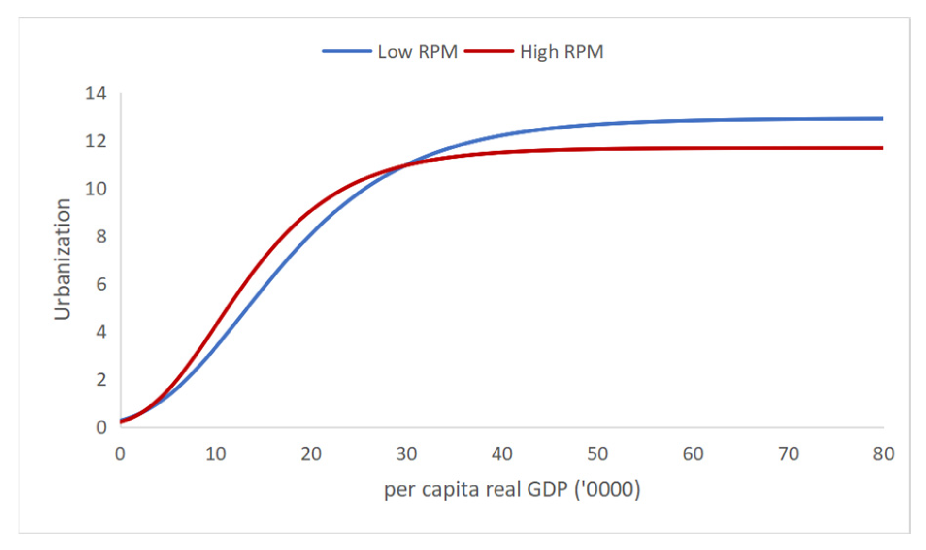
Analysis continued by examining how different RPM conditions influenced the relationship between income and urbanization, as presented in Models D1 and D2 in Table 5. As shown in Figure 14, at low income, high RPM conditions slightly favored urbanization compared to low RPM conditions (aligning with M2); however, when income exceeded a specific threshold, low RPM conditions typically corresponded with higher urbanization levels and saturation points compared to high RPM conditions (corresponding to M3). This phenomenon aligns with industrialization-driven structural transformation and evolving transport demands, as illustrated in Section 3. As Duranton and Turner [81] and Donaldson [84] articulated, with rising income, industrialization-driven structural transformation typically shifts the economy from traditional agriculture or resource dependence toward manufacturing and services, resulting in a structural evolution of transport demand. This transition is usually accompanied by greater industrial diversification and suburban expansion, which together generate a surge in demand for flexible, timely, and efficient transport services [85]. According to transport-demand evolution effects (M3), HM roads, with their superior flexibility, mobility, and efficiency, play an unparalleled role in meeting these emerging demands [50,71,81,82].

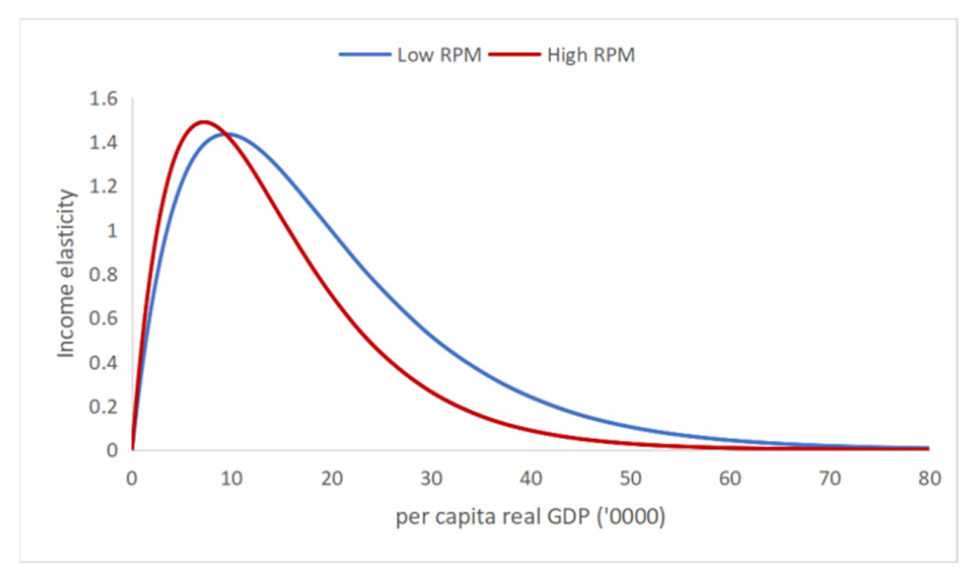
Figure 15 presents income elasticity curves under high and low RPM conditions. Both curves display similar peak values, with high RPM elasticity coefficients slightly exceeding low RPM before reaching their respective peaks. However, notably, income elasticity under low RPM conditions declined more slowly than under high RPM conditions after exceeding peak values, emphasizing more sustainable urban growth under low RPM conditions at higher income levels. This result underscores the importance of HM roads in supporting further urban expansion during higher income stages.

6.2.2. The Interactive Effects of RPM and Low HPA Conditions on Urbanization Patterns

Models E1 and E2 in Table 5 present results of high and low RPM under low HPA conditions on the relationship between urbanization and income. As shown in Figure 16, urbanization curves corresponding to high and low RPM under low HPA conditions differ significantly in shape from urbanization curves for high and low RPM in Figure 13.

Under low HPA conditions, the two curves exhibit markedly different growth trajectories. This disparity arises from inconsistencies in the relative improvements of different LTIs: low HPA with high RPM emphasizes more HA and CR, while low HPA with low RPM focuses on more HA and HM. Before income reaches 50,000 RMB, urbanization levels corresponding to the black curve exceed those corresponding to the blue curve. This pattern is explained by the black curve’s emphasis on developing large-scale basic LTI (HA and CR) within regions, producing pronounced M1 (scale) and M2 (migration) effects. As previously discussed, these two transport types are crucial for satisfying local economic transport needs and industrialization-driven transport demand [81]. The blue curve, emphasizing more HA and HM while underestimating CR’s role in early industrialization, delays urbanization processes at lower income levels [61,86,87]. This result strongly underscores the indispensable role of a transport configuration that combines more HA roads and CR in fostering urbanization during low- and middle- income stages.

However, after income surpasses 50,000 RMB, the blue curve, compared to the black curve, experiences faster, steeper urbanization. This implies that at higher income levels, a transport configuration that emphasizes more HA and HM roads instead of more HA roads and CR is better matched to M3, thereby delivering faster urbanization. This difference arises from the structural shift in transport demand at higher income levels, driven by greater social specialization, industrial diversification, and the spatial expansion and dispersion of cities, thereby generating large-scale demand for more flexible road transport services [71,82]. This result further emphasizes the importance of HA roads and CR in lower income stages, and HM roads in higher income levels for advancing urbanization processes [60,88].

Figure 17 reveals income elasticity curves under low HPA conditions for high RPM (black, with smaller peak) and low RPM (blue, with higher peak). At lower income levels, the blue curve’s elasticity values significantly exceed those of the black curve. However, during higher income stages, the black curve’s elasticity values exceed those of the blue curve, as the blue elasticity curve declines more rapidly after reaching its peak. An interesting yet seemingly contradictory trend emerges here. Under low HPA conditions, despite lower urbanization levels during higher income stages, high RPM corresponds with more sustainable urban growth. This significant finding emphasizes CR’s importance during this stage; despite its limited flexibility, its advantages in mobility, capacity, and long-distance transport make it an important complement to HM roads [60,74,89].

6.2.3. The Interactive Effects of RPM and High HPA Conditions on Urbanization Patterns

Models E3 and E4 compared how high and low RPM influenced the relationship between income and urbanization under high HPA conditions, as shown in Table 5. As depicted in Figure 18, under high HPA conditions, high RPM corresponds with higher urbanization levels at lower income levels, while low RPM scenarios achieve even higher urbanization saturation levels at higher income levels. This result emphasizes that under high HPA conditions, although low RPM urbanization growth may be slower, it achieves higher saturation points. This phenomenon highlights the complex influence mechanisms between LTI supply and economic demand that continuously evolve across economic development stages.

Under high HPA and low RPM conditions, LTI constitutes “more HSR and HM roads with relatively fewer CR and HA roads,” while under low HPA and high RPM conditions, it constitutes “more HSR and CR with relatively fewer HM and HA roads.” This structural difference creates different supply characteristics, subsequently influencing urbanization processes. During mid income stages, the black curve under the latter condition features more CR, resulting in more apparent urbanization progress, while the red curve under the former condition has less CR, causing slower urbanization, highlighting the migration-transition role of CR (M2).

However, during higher income levels, combinations primarily relying on HSR and CR face supply–demand mismatches. While HSR provides efficient passenger transport, its limited station flexibility constrains its ability to meet diverse and adaptable regional transport needs compared to HM roads, weakening urbanization momentum [52,90]. By contrast, the “more HSR and HM” combination shows clear advantages in higher income stages, aligning with M3 (transport-demand evolution) and M4 (service-quality optimization) and confirming the synergistic effects between these two modes. HM roads address flexible transport needs over medium-to-short distances with high frequency and small batches, while HSR serves long-distance, high-value, time-sensitive demands, together forming a diversified LTI supply structure [55,91,92]. Therefore, the synergistic effects foster higher levels of urbanization by enhancing the efficiency, adaptability, and connectivity of the urban economic environment [90,93]. Notably, the urbanization saturation level under high HPA and low RPM conditions is significantly higher than that of all other LTI combinations, offering new insights into achieving more advanced levels of urbanization.

Figure 19 reveals income elasticity curves under high HPA conditions for high RPM (black) and low RPM (red). At lower income stages, elasticity values on the black curve are notably higher than those on the red curve. In contrast, at higher stages, the red curve surpasses the black, which declines more rapidly after its peak. Moreover, under low RPM conditions, elasticity approaches zero at much higher income levels than under high RPM, despite lower peak values. This suggests that sustainable urban growth under low RPM conditions outperforms high RPM, highlighting the critical role of more HSR and HM in supporting sustainable urbanization at later income stages.

6.3. The Impact of Relative Improvements in MPA on Urbanization Patterns

Finally, this study analyzed the impact of MPA on the relationship between income and urbanization growth patterns, as shown in Models F1, F2, and F3 in Table 6. As depicted in Figure 20, during lower income stages, urbanization levels were higher under low MPA conditions compared to high and mid MPA conditions (corresponding to M1 at lower incomes). However, once income exceeded a specific threshold, mid MPA conditions typically corresponded with higher urbanization levels (aligning with M3 at higher incomes). These findings suggest that a more harmonious road network (including both HA and HM roads) played a vital role in meeting diverse transport demands. Meanwhile, the figure also reveals an interesting trend: under high MPA conditions, both the urbanization growth speed and saturation level were the lowest, indicating that excessive expansion of HM roads can be detrimental to urbanization.

The “high-MPA trap” via sprawl and network imbalance. A persistently high MPA signals over-investment in HM roads relative to HA roads. Within our framework, M1 is weakened because dispersed, auto-oriented growth dilutes market thickness and raises unit logistics/commuting costs. In early-mid income contexts, expanding HM roads tends to stretch the urban footprint and promote automobile-oriented sprawl, which spreads jobs and residences, reduces land-use efficiency, and increases the per capita cost of infrastructure and public services—thereby eroding agglomeration benefits that underpin urbanization [94]. M2 is impeded by induced travel: new HM roads generate additional vehicle kilometers, so congestion relief is short-lived while car dependence deepens. When the HA network lags, overbuilding expressways produces a hierarchical imbalance that prioritizes long-haul speed over door-to-door accessibility, slowing the conversion of rural migrants into settled urban residents [95,96]. M3 is mis-served because the portfolio prioritizes fast trunks but under-provides the middle/last-mile capacity needed for dense, high-frequency metropolitan trips; this advances the turning point on the urbanization curve and lowers subsequent responsiveness [97,98]. Finally, M4 deteriorates when HM roads expansion crowds out maintenance and upgrades for HA roads, heightening congestion and externalities. Sprawl-prone form is associated with higher transport energy use and worse air pollution exposure, which feed back into slower productivity and livability, thus lowering the saturation level of urbanization. Recent studies link dispersed form to elevated CO₂/PM_2.5 burdens, while more compact morphology improves environmental performance [7,33,99].

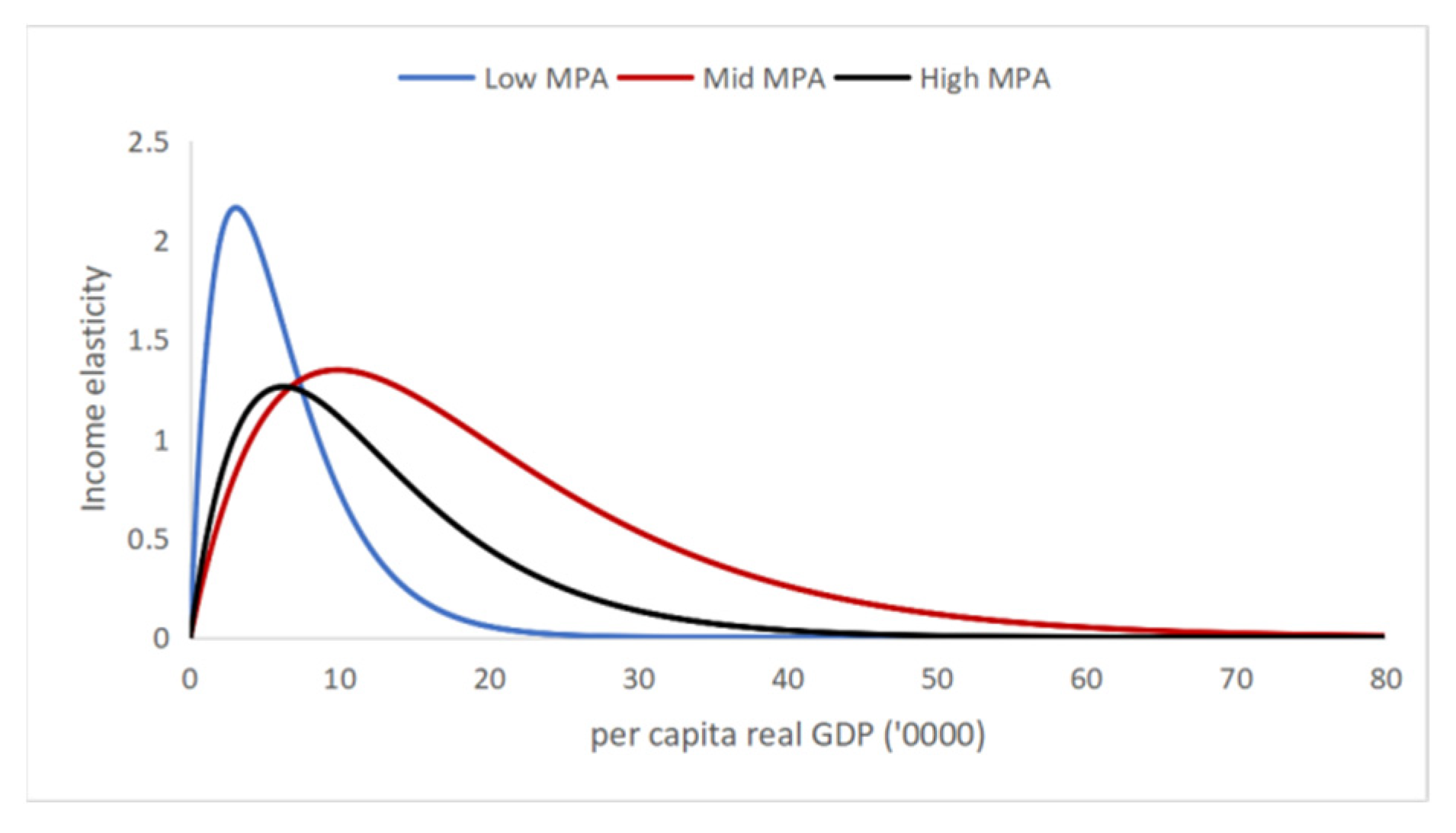
Figure 21 displays income elasticity curves under three MPA conditions. At lower income, income elasticity under low MPA conditions consistently exceeded that under mid and high MPA conditions. However, after reaching peak values, elasticity curves under low MPA conditions approached zero much faster than under mid and high MPA conditions. A noteworthy observation is that the blue curve exhibits the highest maximum elasticity coefficient among all three MPA conditions, once again emphasizing the importance of more HA roads for urbanization at lower income levels. Additionally, the red curve consistently exceeds those under low and high MPA conditions at higher income levels, aligning with previous findings that highlight the value of a balanced road network in meeting diversified economic demands as economies progress [58]. In contrast, the black curve remains consistently below the red curve, indicating that excessive HM roads development contributes less to urbanization than a more balanced construction strategy—providing valuable insights for transport policy.

Table 7. Effects of LTI and income stages on urbanization patterns.

Dominant Portfolio of LTI	Income Stage		Saturation
	Lower Income	Higher Income
	Elasticity	Elasticity
Low RPA	↑	↓	↓
High RPA	↓	↑	↑
Low RPM	↓	↑	↑
High RPM	↑	↓	↓
Low MPA	↑	↓	↓
Mid MPA	↓	↑	↑
High MPA	↓	↓	↓
Low HPM	↑	↓	↓
High HPM	↓	↑	↑

,

Table 8. Interaction effects of LTI portfolios on urbanization elasticity and saturation across income stages.

Income Stage	Mode Pairing	Elasticity	Saturation	Policy
Low income	HA and CR (accessibility)	↑	→	Expanding first/last-mile access, county–township connectivity and basic haul capacity—consistent with New Urbanization, Urban–Rural Integration, and Rural Revitalization.
Middle income	CR and HM (capacity and flexibility)	↑ (peak)	↓	Building feeder and intercity corridors, advancing Coordinated Regional Development.
High income	HSR and HM (quality and integration)	→	↑↑ (most sustainable)	Promoting High-quality New Urbanization, mature-cluster coordination, and dual-carbon objectives.

and

Table 9. High MPA and low RPA with high HPM on urbanization elasticity and saturation.

Mode Pairing	All Income Stage		Policy
	Elasticity	Saturation
High MPA	↓	↓	Keep MPA in low–mid band; pair HM additions with HA/CR to limit sprawl/induced traffic; set MPA upper bound.
HA and HSR (low RPA and high HPM)	↓	↓	HSR expansion conditional on feeder readiness (CR/HM and station-area access); avoid premature HSR without feeders.

synthesize the sequence of modal salience as income rises. For each stage, it lists the dominant portfolio (mode pairing) and the relative movement in income elasticity and saturation level. Arrows indicate within-stage, cross-portfolio comparisons: ↑higher, →similar, ↓lower. Table 7 reports the stage-specific effects of individual LTI categories on saturation level and income elasticity. The sequence of modal salience with rising income is HA → CR → HM → HSR. Table 8 synthesizes the portfolio-level response by income stage, showing how the dominant mode pair shifts as income rises: HA + CR → CR + HM → HM + HSR. For each stage, the table summarizes the relative movements in saturation and elasticity across portfolios. Table 9 documents composition pitfalls in the interaction of LTI and income: (i) high MPA is associated with lower saturation and elasticity than mid- and low-level MPA, and (ii) under low RPA, high HPM underperforms, consistent with a strong-trunk/weak-feeder mismatch. These patterns flag configurations that are counterproductive for urbanization.

To assess robustness, the main specifications were re-estimated under alternative cutoffs. Results are unchanged: coefficient signs and significance, the stage ordering (HA → CR → HM → HSR), the “high-MPA trap,” and the “low-RPA and high-HPM penalty” all persist; shifts in elasticities and saturation parameters remain within the baseline 95% confidence intervals, and fit metrics vary only marginally. Full estimates are reported in Tables S6–S8.

7. Conclusions

This study extends previous research by examining the impacts of relative improvements in various LTI types and their interactive effects on the relationship between urbanization and economic performance. Methodologically, the paper introduces a ratio-based portfolio lens and a Gompertz–income reading that summarizes urbanization dynamics. A logistic S-curve re-estimation provides cross-validation, confirming that core patterns are robust to the functional form. Using provincial panel data (2000–2022) and Gompertz models, the estimated urbanization growth rate approaches zero at around RMB 600,000 per capita, consistent with a saturation level (12.2); the peak income elasticity is 1.39 at about RMB 90,000 per capita. Across income stages, the sequence of modal salience is HA → CR → HM → HSR, reflecting a transition from basic access (M1) to migration-led scale effects (M2), then to demand evolution and network flexibility (M3), and finally to service-quality optimization (M4).

Empirically, four salient features warrant emphasis. (i) At lower incomes, lower RPA (more HA relative to CR) is associated with higher urbanization levels, consistent with the role of first/last-mile access and basic market integration (M1). With rising income, higher RPA (more CR) corresponds to higher saturation and sustained growth, in line with migration transition and medium-/long-haul needs (M2). Comparable patterns are observed for RPM and MPA as well: for RPM, mixes favoring HM over CR become advantageous at higher incomes but not at lower ones; for MPA, mid-level portfolios outperform both low and high at higher incomes, whereas low MPA performs better at lower income levels. (ii) The “high MPA trap” emerges: very high HM relative to HA (high MPA) is associated with a lower attainable ceiling and earlier deceleration than mid MPA, indicating overemphasis on fast trunk mobility at the expense of access and feeder capacity (M1–M4). (iii) A high-HPM, low-RPA mix yields the lowest urbanization saturation and the slowest growth across income levels, because thin CR/HM feeders prevent HSR’s line-haul advantages from translating into door-to-door accessibility, producing a trunk-feeder imbalance and weakening M2–M4. (iv) Portfolio interactions are stage-contingent: HA + CR dominates at low income (M1–M2), CR + HM at middle income (M2–M3), and HSR + HM at higher income provided feeder integration is in place (M3–M4). Elasticity patterns mirror these shifts, with peak responsiveness moving from HA/CR to CR/HM and finally to HSR/HM as income rises.

For policy, the findings support a stage-matching principle that optimizes the relative composition of LTI rather than pursuing uniform expansion, and they map cleanly onto China’s policy frameworks. At low income, prioritize HA roads and CR to expand first/last-mile access, county–township connectivity, and basic haul capacity—consistent with New Urbanization (people-centered, service equalization), Urban–Rural Integration, and Rural Revitalization/Four-Good Rural Roads. At middle income, pivot to CR and HM roads to build the “missing-middle” (feeder and intercity corridors) and implement trunk–feeder separation, advancing Coordinated Regional Development and the National Comprehensive Multimodal Transport Plan (2021–2035). While keeping MPA within an upper bound to avoid sprawl-prone growth. At high income, integrate HSR and HM roads conditional on feeder readiness (CR/HM links and station-area access), advance transit-oriented development and transport demand management; this supports high-quality new urbanization, mature-cluster coordination (e.g., Jing-Jin-Ji, Yangtze River Delta, Greater Bay Area), and dual-carbon objectives.

Several limitations qualify the interpretation of the findings. (1) Endogeneity. Two-way causality is plausible—higher incomes can finance more LTI, while LTI can influence urbanization and income—and omitted factors (e.g., governance quality, land and housing policy, industrial upgrading, environmental regulation, digital connectivity, demographic change, cross-provincial spillovers) may co-vary with both LTI and urbanization. These channels can bias the estimated income–urbanization elasticities and the moderating effects of LTI portfolios. Ratio-based LTI measures and multiple specifications reduce—but do not eliminate—these risks. Results are therefore best interpreted as conditional associations consistent with stage matching, rather than causal effects. (2) Spatial scale and heterogeneity. Using provinces as the unit of analysis may mask within-province variation (urban belts, corridor segments, station catchments) and raises modifiable areal unit problem concerns. Cross-border spillovers along corridors are only captured indirectly. (3) Outcome scope. The analysis focuses on the income–urbanization path and does not explicitly model environmental externalities or energy use. Road-heavy portfolios may increase transport energy intensity and PM_2.5 exposure via induced travel and sprawl, while HSR benefits may depend on carbon intensity and station–area accessibility. Estimates should therefore not be read as a full welfare assessment. (4) Because of limited sample size and panel–balance constraints (finite provincial observations), a formal holdout or k-fold stability check was not feasible; future work using larger, city-level panels could implement cross-validation to assess parameter stability.

Future research can address these limitations along three aligned fronts: (i) Identification. Employ instrumental-variables strategies (e.g., historical rail alignments, terrain-based least-cost paths, planned-but-not-built segments, budget/policy shocks), event-study or staggered DiD around HSR/expressway openings, dynamic panel (system-GMM) to handle persistence and feedback, and sensitivity/bounds analyses for residual selection (e.g., Oster-type diagnostics). (ii) Spatial resolution and spillovers. Move to city/county panels and corridor/station-catchment buffers; implement spatial econometric models (SAR/SDM/SARAR) to capture spillovers; conduct multi-scale and alternative zoning robustness checks to assess the modifiable areal unit problem; and consider multilevel (hierarchical) specifications to separate within- and between-province variation. (iii) Multi-dimensional outcomes. Extend outcomes to a “quality of urbanization” index (e.g., PM_2.5 exposure, transport CO₂ intensity, land consumption per capita, congestion delay, accessibility equity); incorporate policy and market moderators (carbon targets, fuel prices, congestion/parking policies); and evaluate portfolio designs under environmental constraints using spatial panels or event-study designs.