The Pandemic and the City: Empirical Evidence of Lifestyle and Location Preference Changes in Japan

Abstract

This study examines how individuals’ preferences for four types of urban functions—residential, work-related, transportation, and leisure—shifted in Japan following the COVID-19 pandemic. We find that the widespread adoption of remote work, mainly in large cities, strengthened preferences for residential amenities while reducing the importance of work-related and transportation functions. In contrast, smaller cities with limited infrastructure experienced more modest changes. Our analysis further reveals that, in metropolitan areas, preference shifts are less strongly associated with local and surrounding amenity conditions, suggesting more complex internal dynamics. By comparison, in smaller cities, the scarcity of amenities makes them play a greater role in shaping these changes.

1. Introduction

“Urban structure” refers to the spatial arrangement of population, infrastructure, and economic activities. In urban economics, two main theoretical frameworks are used to explain how population distribution emerges: the production-based theory [1], which centers on commuting needs and productivity, and the consumption-based theory [2,3], which emphasizes demands for consumption amenities. In the latter, urban form is shaped less by workplace proximity and more by residents’ utility-maximizing choices, reflecting evolving social, economic, and lifestyle demands.

Urban structures are not static but evolve over time due to shifts in technology, preferences, and external shocks. Understanding these dynamics is essential for policymakers aiming to design adaptive and sustainable cities. Recent studies highlight that technological advancements, particularly in information and communication technology (ICT), have enabled more mobile work styles, reshaping urban form and residential behavior [4,5]. However, such technological impacts often unfold gradually and are heavily dependent on infrastructure investment.

In contrast, urban planning and major shocks such as natural disasters or pandemics can cause rapid shifts in urban population distribution. Glaeser [6] argues that while disasters may cause short-term disruptions, urban planning exerts more persistent effects on city form. Nevertheless, significant events such as earthquakes, tsunamis, or pandemics can temporarily alter population distributions before eventual reversion to pre-disaster equilibria, as they do not fundamentally change how people evaluate locations and amenities.

The COVID-19 pandemic, as a major global public health crisis, has dramatically influenced urban dynamics, including housing markets [7,8,9], work productivity [10], and population distribution [11,12,13,14]. While some changes are temporary, such as those driven by infection fears or lockdowns, others, notably the spread of remote work, appear more persistent. Monte et al. [15] establish a theoretical urban model with an endogenous remote work choice, showing that this shift in work modes leads to changes in preferences. Combined with empirical evidence, their study suggests that changes in population distribution may be persistent in megacities but only temporary in smaller cities. Their findings underscore how changes in the individual valuation of urban functions can reshape spatial structure.

In Japan, a country with extensive experience in both modernization and disaster resilience [16,17], the pandemic similarly affected urban spatial dynamics. Policies encouraging remote work and public health investment catalyzed changes in behavior. However, most existing studies in Japan focus on infection trends [18], vaccination [19], mobility patterns, or productivity impacts [20], whereas only a few, such as Arimura et al. [21], explore changes in population distribution in Japan.

While the former contributions are important, they offer limited insight into a more fundamental question: where do people prefer to reside during and after the pandemic, and how have their preferences evolved? To address this question, the present study adopts a preference-oriented approach grounded in a consumption-based perspective to examine changes in individual preferences for four core urban functions: residential, work-related, transportation, and leisure. By combining high-resolution population data from LandScan with amenity data from TelPoint and applying geographically weighted regression (GWR) across 33 Japanese cities, this study captures the lifestyle changes that took place after the COVID-19 pandemic, providing new insights by examining how preference shifts vary across urban contexts, shaped by underlying amenity conditions and the spread of remote work practices. In particular, this study sheds light on both the spatial patterns and potential mechanisms of these changes. Its findings aim to inform ongoing discussions on urban planning in the post-pandemic period, particularly in light of Japan’s long-term demographic trends.

We present the following key findings: first, residential preferences have strengthened, while preferences for work-related and transportation amenities have weakened, indicating a persistent shift towards remote work lifestyles. These changes exhibit distinct spatial patterns, particularly in large cities, where preference dynamics are less predictable based on local amenity conditions than in smaller urban centers.

The remainder of this paper is structured as follows: Section 2 reviews the relevant literature on Japan’s urban structure. Section 3 describes the dataset and methodology. Section 4 presents the empirical results. Section 5 discusses the empirical results and policy implications. Section 6 concludes the paper with empirical results and implications.

2. Literature Review

2.1. Population Distribution in Japan

Japan has a long history of urban development, its urbanization beginning earlier than in China and Korea, as shown in Figure 1. Its capital, Edo (modern-day Tokyo), is believed to have had more than one million residents as early as the 18th century [22]. Today, Tokyo remains the most populous city globally. The foundation of Japan’s modern urban structure began with the Meiji Restoration in 1868, marking a shift from feudal society to industrialization. During this period, urban growth was concentrated around key industrial and port cities such as Tokyo, Osaka, and Nagoya, shaped by national policies aimed at rapid industrial expansion.

Following continued industrialization and infrastructure investment, Japan’s urbanization rate exceeded 20% in the 1900s and has since risen to 71.4% [23]. Several megacities have developed across different regions, including Fukuoka in Kyushu and Sapporo in Hokkaido, as shown in Figure 2. As of today, the Tokyo–Nagoya–Osaka Corridor has been the most important economic and production engine in Japan, with a population of over 60 million. Within this city cluster, over 37 million people reside in the Greater Tokyo Area.

Alongside urban expansion, Japan frequently faces natural disasters, particularly earthquakes and tsunamis, which substantially impact urban reconstruction and residential preferences. For instance, Naoi et al. [24] show that earthquake risk affects housing prices, reflecting changes in perceived preferences regarding disaster risk. Similarly, Chang [25] finds that although the city’s population recovered after the 1995 Kobe Earthquake, the distribution shifted away from the historical center to peripheral areas. Kondo and Lizarralde [26] analyze post-disaster migration following the 2011 Great East Japan Earthquake and Tsunami, revealing increased urban sprawl and fragmented spatial patterns driven by uncertainty about future hazards.

In summary, Japan experiences various disasters, and urban structures and population distribution are evolving alongside processes of urban resilience and reconstruction. However, as opposed to physical natural disasters such as earthquakes and tsunamis, the COVID-19 pandemic is a global public health disaster, and its impact is not limited to specific regions.

2.2. COVID-19 in Japan

The COVID-19 pandemic has reshaped urban structures and population distribution in various aspects, as documented in Section 1. This section introduces the current studies about COVID-19 in Japan. From the weekly confirmed cases shown in Figure 3, it can be observed that Japan maintained low infection levels during the initial stage of the pandemic. However, a significant surge occurred from 2022 to 2023, with cases peaking in mid-2022 before gradually declining to lower levels by 2024. In the early outbreak, the Japanese government announced self-regulation and a voluntary lockdown. Watanabe and Yabu empirically identify that citizens refrained from going out in line with the government’s request [27,28]. Furthermore, Watanabe [29] and Iwasaki et al. [18] provide evidence that population distribution patterns in Japan contributed to keeping infections under control. After the early outbreak, scholars began discussing vaccination and reviewing the spread of infections. Machida et al. [30] provide a timely report on the low vaccination acceptance rate, investigating which groups were hesitant to get vaccinated and the historical reasons behind this. Even recently, Tokumoto et al. [19] mentioned the effect of vaccination and discussed infection distribution in both time and space from 2020 to 2023.

Beyond public health, a growing body of studies explore urban mobility as a proxy for population distribution and preferences. For example, Nomura et al. [31] utilize mobile phone data to show that infection rates significantly reduced nighttime population densities, suggesting behavioral adaptation, and Okamoto [32] uses Google mobility data to analyze time spent at home versus outside across different phases of the pandemic, though their study is limited to predefined locations.

3. Data and Methodology

3.1. Data

This study employs two primary datasets: population density and urban amenity information. For population density, we use the LandScan Global Population Dataset, developed by the Oak Ridge National Laboratory (Oak Ridge National Laboratory, TN, USA). LandScan provides high-resolution estimates of ambient population density at approximately 1-kilometer resolution, derived through a combination of census data and remote sensing. A key limitation of LandScan is that it represents a 24-h average population, without distinguishing between daytime and nighttime patterns. As a result, it does not allow for precise analysis of employment- or residence-specific distributions by time of day.

Despite this constraint, LandScan is widely adopted in multi-city and cross-regional urban studies. For example, Li et al. [33] use LandScan to investigate the relationship between polycentricity and air quality. Similarly, Zhang et al. [34] examine the evolution of urban population distribution in Shanghai, and Li et al. [35] use it to analyze structural urban changes across 300 Chinese cities. In the Japanese context, Uchiyama and Mori [36] employ this dataset to assess sustainability indicators in major cities, including Tokyo and Osaka.

With the awareness that Japan maintains detailed official census and migration data through the Ministry of Internal Affairs and Communications, this study employs LandScan data for several reasons. First, LandScan is updated annually, whereas Japanese census data are released at five-year intervals. This allows us to draw on a time series covering 2016, 2019, 2020, and 2022, thus capturing both the pre-pandemic and post-pandemic urban structure. Second, although Japanese census data offer a finer spatial resolution (500 m), LandScan’s resolution is sufficiently fine for this study, particularly given its annual updates.

Given Japan’s aging population and the concentration of activity in metropolitan regions, many smaller municipalities exhibit limited urban area and sparse amenity coverage. As such, in order to ensure reliable estimation and reduce spatial bias, we limit our analysis to cities with populations exceeding 500,000. This yields a total of 33 cities (as shown in Figure 4), including major metropolises (e.g., Tokyo, Osaka, Kyoto), suburban cities near Tokyo (e.g., Funabashi, Kawaguchi), and key regional centers in Kyushu and Hokkaido (e.g., Fukuoka, Sapporo). The detailed city list is provided in Appendix A.1.

For urban amenities, we utilize TelPoint data provided by Zenrin Fukuoka, Japan, a comprehensive database of businesses in Japan derived from the NTT phone book, one of the most inclusive business directories in Japan. Also known as the NTT Town Page, it has historically been published by NTT and lists businesses and public institutions, together with their telephone numbers, addresses, and occasionally business hours or services. Zenrin uses it to further verify each entry and geocode its location. Although the dataset initially contained only landline registrations, recent versions no longer rely exclusively on fixed-line phones. According to its technical manual, TelPoint also records mobile phone numbers, PHS, and toll-free lines. Thus, facilities are not restricted to landline telephones.

This dataset contains various information, including precise coordinates and industrial categories, of which there are 39 primary, ranging from agriculture, fabric, and manufacture industry to financial and public services. For analytical simplicity, we select life-related types and group them into four urban amenity types, namely residential, leisure, work, and transportation, defined in

Table 1. Definition of amenity types.

Variable	Definition	Measure
Residential	Real estate agency, life-related (convenient store and so on), medical amenity, education	Number within area
Work	Finance, professional skills, business, public service	Number within area
Trans	Metro station, subway	Distance from the closest
Leisure	Sports, entertainment and foods, resorts	Number within area

Source: table created by authors.

.

We adopt a fourfold framework—residential, work, transportation, and leisure—for both theoretical and practical reasons. This framework originated with Le Corbusier, but has been criticized for its oversimplification [37]. We acknowledge this criticism; however, these categories remain closely aligned with the core perspectives in urban economics: housing and workplace location [1,3], transport accessibility, and consumption amenities [38]. Thus, from a methodological standpoint, aggregating amenities into these four broad categories ensures tractability and interpretability while allowing for meaningful cross-city comparisons across 33 cities. Recent empirical studies also employ similar groupings when analyzing population distribution and amenity preferences [39,40]. We therefore regard the fourfold framework as a pragmatic yet theoretically grounded approach for capturing preference shifts in this study.

In order to reveal the heterogeneity of urban structure shifts and investigate the mechanisms, the following analysis focuses on two groups—top and other—as defined in Appendix A.1. Summary statistics for the dependent variable and four amenity categories are presented in

Table 2. Summary statistics.

Group	Variable	2016			2019			2020			2022
		Mean	Ineq	Moran	Mean	Ineq	Moran	Mean	Ineq	Moran	Mean	Ineq	Moran
Average city	population	3336.48	0.54	0.70	3299.45	0.54	0.70	3366.26	0.54	0.70	3406.05	0.54	0.71
	leisure	23.35	0.77	0.27	20.01	0.77	0.28	18.61	0.77	0.28	17.98	0.77	0.28
	residential	52.87	0.70	0.43	47.99	0.70	0.43	44.49	0.70	0.44	43.50	0.70	0.44
	transport	3373.75	0.44	0.84	3550.28	0.44	0.85	3620.19	0.43	0.85	3787.71	0.42	0.85
	work	14.15	0.76	0.33	12.73	0.77	0.32	12.07	0.77	0.32	11.80	0.77	0.32
Top city	population	5707.86	0.39	0.68	5646.55	0.39	0.68	5824.36	0.39	0.68	5918.83	0.40	0.69
	leisure	52.88	0.72	0.36	45.09	0.72	0.37	42.45	0.72	0.37	40.45	0.72	0.38
	residential	106.30	0.61	0.49	95.23	0.61	0.49	89.41	0.60	0.49	86.27	0.60	0.49
	transport	1407.13	0.58	0.78	1629.86	0.57	0.79	1730.40	0.54	0.80	1732.42	0.54	0.79
	work	33.42	0.74	0.46	29.46	0.75	0.45	28.10	0.75	0.44	27.13	0.75	0.44
Other city	population	2767.35	0.58	0.71	2736.15	0.58	0.71	2776.32	0.58	0.71	2802.98	0.58	0.71
	leisure	16.27	0.78	0.25	13.99	0.78	0.25	12.89	0.78	0.25	12.58	0.78	0.26
	residential	40.04	0.73	0.42	36.65	0.73	0.42	33.70	0.72	0.43	33.23	0.72	0.43
	transport	3845.74	0.41	0.86	4011.17	0.41	0.86	4073.74	0.40	0.86	4280.98	0.40	0.86
	work	9.53	0.77	0.30	8.72	0.78	0.29	8.23	0.78	0.29	8.13	0.78	0.29

Source: summary statistics table created by authors.

, reported at the average level for three panels: the Average panel shows the full-sample mean, the Top panel covers the cities in the top group, and the Other panel includes the remaining cities.

The table reveals significant disparities between the top and other groups. The population density in top-tier cities is more than twice that of other cities, and top cities exhibit considerably richer amenity resources, particularly in leisure- and work-related categories. Additionally, the average distance to the nearest metro station is notably shorter in top cities, indicating better transport accessibility. Inequality measures suggest a more balanced distribution of residential, leisure, and work-related amenities within top cities compared with the other group, reflecting the more advanced infrastructure and well-distributed urban demand in major metropolitan areas, which contribute to a more equitable spatial layout of amenities and higher baseline accessibility.

3.2. Methodology

This study consists of two primary phases of empirical analysis. In the first phase, spatially varying preferences for four amenity types are estimated using geographically weighted regression to capture both overall trends before and after the COVID-19 outbreak. In the second phase, we examine the spatial patterns and mechanisms underlying these preference changes through Pearson’s correlation coefficient and an exploratory model. Given the inclusion of over 30 Japanese cities, we classify the sample into two groups, as illustrated in the previous subsection. This study utilizes both ArcGIS Pro version 3.5 (Esri, Redlands, CA, USA) and R version 4.4.2 (R Foundation for Statistical Computing, Vienna, Austria). The flow of analysis is summarized into Figure 5:

3.2.1. GWR: Preference Estimation

Preference is an abstract and unobservable concept that cannot be directly derived from population or amenity data. In empirical studies, it can be revealed through willingness to pay (WTP) using a hedonic approach [41]. Hedonic models decompose the equilibrium price of a good (e.g., housing) into the marginal contributions of its attributes. In this framework, the estimated coefficients reflect the WTP for specific attributes, such as proximity to amenities (For example, housing price studies commonly find that property values decline with increasing distance from metro stations, implying a stronger preference for transport accessibility). A similar logic can be extended to population density, which reflects the revealed location choices of residents. A specific type of amenity being positively associated with population concentration suggests a spatial manifestation of preference for that amenity type. In this context, amenity impacts on population distribution can serve as a valid proxy for preference, in a similar manner to the WTP estimated in hedonic models.

This conceptual framework has been applied in previous studies. For instance, Izon et al. [42] show that natural amenities such as green spaces do not always increase population density, highlighting that residents not only evaluate the presence of amenities but also their accessibility and quality. Similarly, Li et al. [39] and Zeng et al. [40] estimate spatial regressions to evaluate how preferences for different amenities evolve in response to structural or social changes. Building on this approach, the present study treats the estimated marginal effects of amenity accessibility on population density as indicators of preferences, which can be locally tracked.

When conducting regression across space, we usually encounter spatial dependence and heterogeneity. These effects can bias coefficient estimates and reduce efficiency if not properly addressed. While a variety of parametric spatial econometric models—such as the spatial lag model (SLM), spatial error model (SEM), and spatial Durbin model (SDM)—have been developed to correct for spatial dependence, they typically assume globally constant parameters and thus are less capable of capturing spatial heterogeneity.

To capture these spatially varying relationships between population density and amenity access, this study adopts geographically weighted regression. As a non-parametric local regression technique, GWR estimates a separate regression at each spatial unit (grid or point) using weighted least squares, where observations closer to the target location receive higher weights. This spatial weighting enables the model to detect localized variations in the strength and direction of amenity effects across space.

Following previous studies [39], this study employs the regression equation as follows:

$$Po{p}_i={\beta }_0(u_i,v_i)+\sum _k{\beta }_k(u_i,v_i){Accessibility}_{ik}+{ϵ}_i$$

(1)

where $Po{p}_i$ is the population density at location i; $(u_i,v_i)$ are the coordinates of location i; and ${\beta }_k(u_i,v_i)$ is the local coefficient of urban function k. This model includes four types of amenities as defined in Table 1.

In this framework, the estimated coefficients ${\beta }_k$ are interpreted as the local preference for amenity type k. For the first three amenity types (residential, leisure, and work), a larger positive coefficient suggests a stronger localized preference, as indicated by higher population density near those amenities. For transportation, measured as distance to the nearest metro station, the coefficient is expected to be negative: a higher absolute value indicates stronger agglomeration around transit nodes, implying a higher preference for transportation accessibility.

3.2.2. Preference Change Pattern Analysis

In addition to conducting GWR, this study further examines the spatial and structural patterns of preference changes and explores the underlying mechanisms that shape these dynamics. Since the GWR model estimates local coefficients for each location, we spatially align the estimation results across different years based on geographic coordinates, allowing for a point-wise analysis of how preferences for different amenity types evolve over time.

This phase pursues two methodological directions. First, we evaluate the interdependencies between changes in different types of preferences by computing Pearson’s correlation coefficients between changes in GWR estimates. This analysis helps to identify patterns of co-occurrence, such as whether declining preference for transportation amenities is systematically accompanied by increased preference for residential or leisure functions.

Second, we investigate the mechanisms underlying preference changes, particularly the extent to which local and neighborhood amenity conditions in 2019 explain the variation in preference changes. Recognizing the presence of spatial autocorrelation, we employ the spatial Durbin model, which accounts for spatial lags in both dependent and independent variables. This approach allows us to separate direct effects from spatial spillovers and offers a more nuanced understanding of how preference dynamics are shaped by local and surrounding areas.

4. Regression Analysis

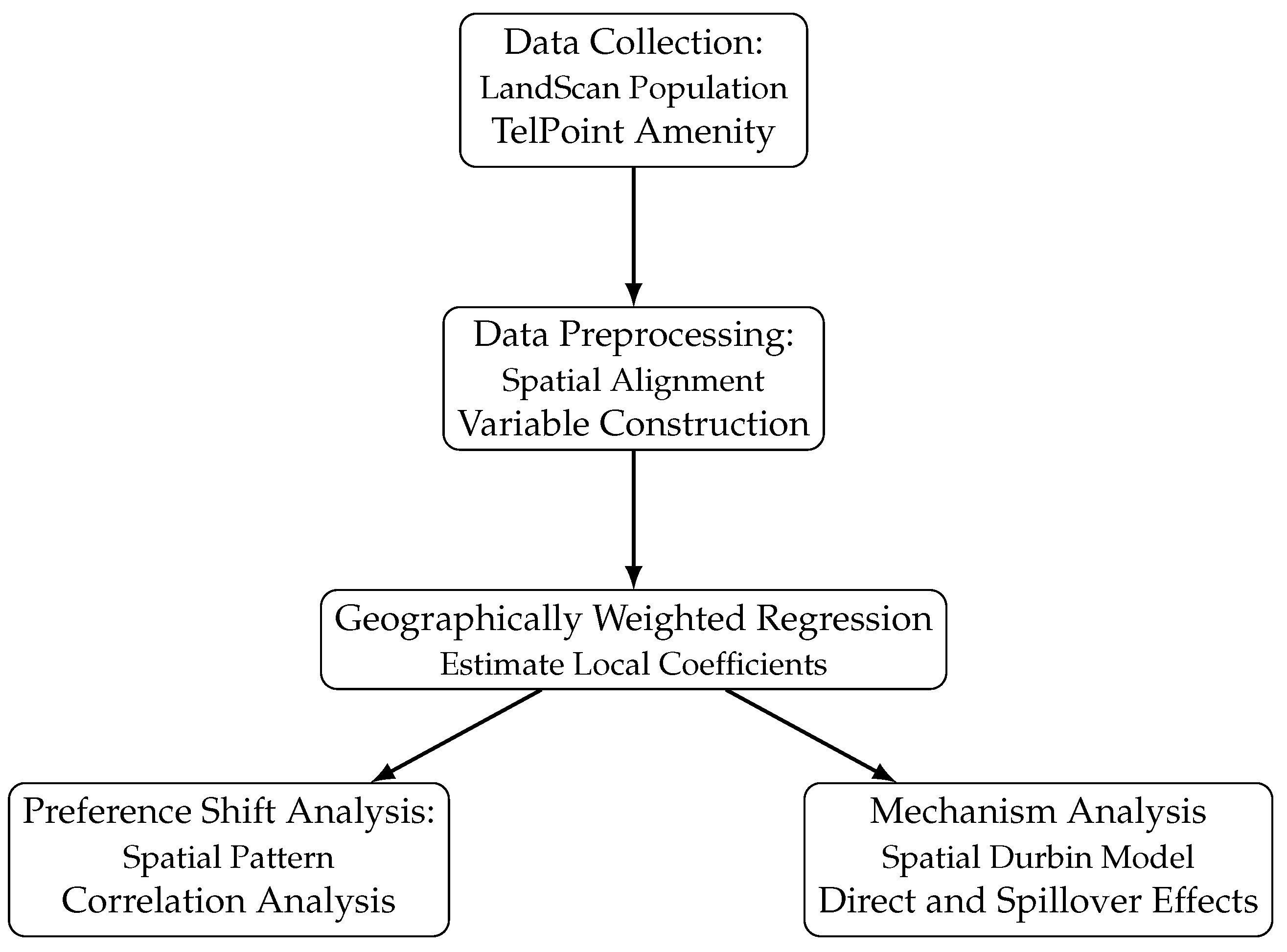
4.1. GWR Estimation

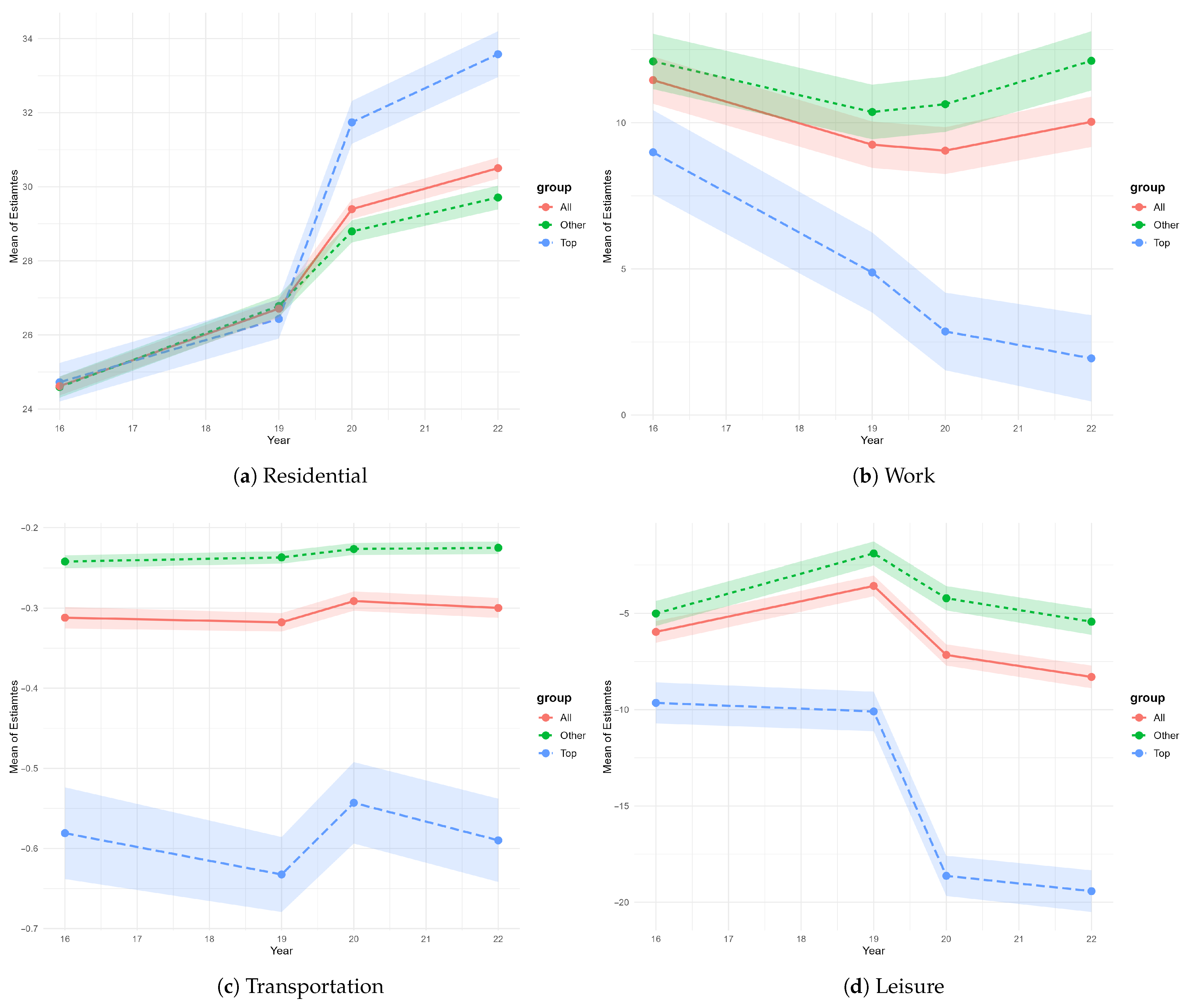
The evolution of amenity preferences is summarized by the GWR coefficient estimates across three groups: the full-sample average, the top cities, and the other cities. We report the group-wise average of the local coefficients in corresponding areas, as shown in Figure 6. Each figure shows the average coefficient over time, with shaded bands representing the 10% confidence interval.

Overall, the GWR estimations reveal that top cities have experienced significant shifts in all preferences, while other cities only exhibit significant preference changes for the residential amenity, which has the most notable and consistent preference shift among all amenity types. Preference for residential functions shows a steady increase prior to the pandemic, and this trend intensifies following the COVID-19 outbreak. Specifically, in top cities, the average coefficient rises from 26.4 in 2019 to 31.7 in 2020, while in other cities, it increases from 26.8 to 28.8 during the same period. Notably, this elevated preference for residential amenities continues even after the relaxation of public health regulations in 2021, suggesting a persistent shift in urban residential preferences.

The evolution of the work preference coefficient reveals distinct patterns between the two city groups. In the top cities, a steady decline in preference for work-related amenities is evident even before the pandemic, with the average coefficient falling from 8.9 in 2016 to 4.9 in 2019. The outbreak of COVID-19 further accelerates this trend, as the coefficient drops to 2.8 in 2020 and reaches 1.9 by 2022. In contrast, the other cities exhibit a more moderate trend. The average coefficient for work amenities rises slightly from 2019 to 2020 and continues to increase modestly through 2022. This suggests that, in less dense or more peripheral cities, the decline in work-related preference is less pronounced, possibly reflecting different degrees of telework adoption or structural change.

The transportation amenity represents a key component of urban infrastructure, particularly in highly developed cities. The coefficients for transportation are expected to be negative, reflecting the population concentration whereby population density decreases as the distance from the transportation amenity increases (This coefficient is often referred to as a gradient, representing the extent of population concentration around a transportation amenity). As shown in Figure 6, there is a notable divergence between the two city groups in terms of both intensity and temporal dynamics.

From 2016 to 2019, the population further concentrated around the transportation amenities in top cities, revealing a stronger demand for the transportation amenity, while such a trend cannot be observed among other cities. Following the outbreak of COVID-19, the preference for transportation accessibility drops sharply in the top cities, falling even below 2016 levels. While the coefficients partially recover from 2020 to 2022, they remain lower than the 2019 level. In contrast, the other cities experience only modest fluctuations, and overall preference for transportation remains relatively stable.

Turning to the leisure amenity, the estimated coefficients are initially negative in both groups. While this may appear unanticipated, given that amenities such as leisure, work, and transit are expected to increase utility, similar patterns have been documented in past research. For instance, Li et al. [39] find that government amenities are negatively associated with population density in Xi’an, and Zeng et al. [40] also report negative coefficients from GWR estimates.

The negative coefficient for leisure may be attributed to collinearity with other amenity types and limitations of the population data. In many cities, leisure, residential, and transportation functions co-locate within mixed-use centers rather than forming distinct zones [43], making it difficult to isolate their individual effects. Additionally, the LandScan dataset captures 24-h ambient population without separating day and night. If interpreted primarily as residential presence, areas with active nightlife or entertainment functions may appear less populated, leading to a downward bias.

Between 2016 and 2019, the preference for the leisure amenity remains relatively stable, with a slight decrease in the top group and a modest increase in the other group. However, following the pandemic, a dramatic shift occurs: in top cities, the coefficient declines from 10.1 in 2019 to −18.2 in 2020, and, similarly, in other cities, it drops from −3.5 to −7.1. These results indicate that leisure-related spaces became substantially less preferred as residential locations during the COVID-19 period, likely due to reduced mobility, behavioral caution, or structural adjustments in urban lifestyles.

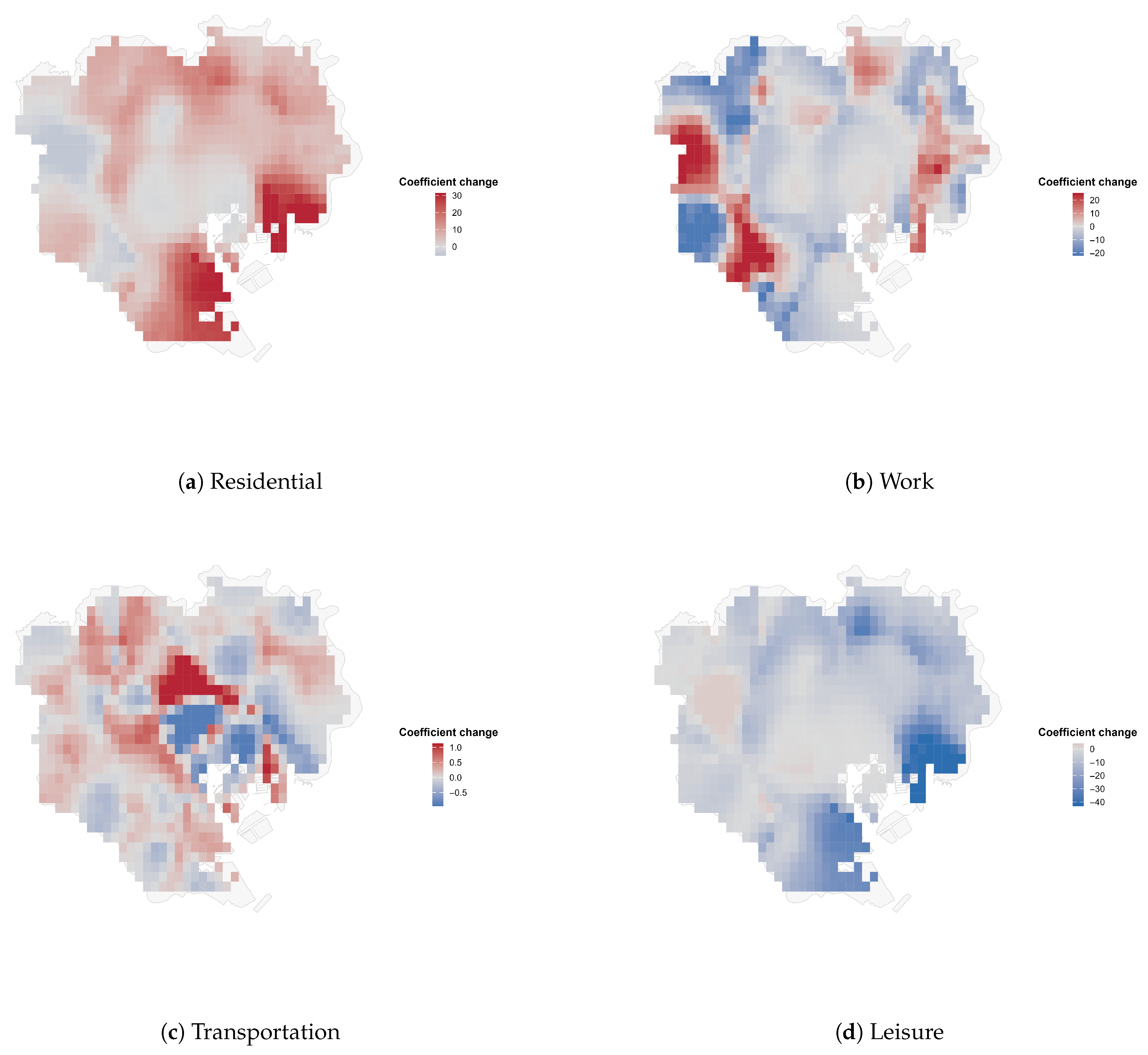
In addition, in Figure 7, we document the geography of preference changes across Tokyo’s 23 special wards between 2019 and 2020. The estimated coefficient changes exhibit clear spatial clustering for all four amenity types. For residential, the changes are predominantly positive and significantly clustered, with the eastern (e.g., Edogawa ward) and southern (e.g., Ōta ward) wards, which are well-connected residential areas, showing particularly strong increases. In contrast, the central business districts of Chuo, Minato, and Chiyoda wards exhibit neutral patterns. Further, the dynamics for work-related amenities reveal an opposing spatial pattern. Preferences remain largely neutral in the central areas but generally decline in the suburban wards. Notably, the preference for transportation accessibility weakens in both the city center and distant suburban areas (e.g., Nerima in the northwest and Katsushika in the east). This decline in the suburbs, which typically rely heavily on transportation amenities for commuting, suggests that the widespread adoption of remote work may have reduced the demand for proximity to transportation amenities. Meanwhile, changes in preferences for leisure amenities are generally neutral to negative across the metropolitan area, with some residential wards experiencing more pronounced declines. Collectively, these spatial patterns provide implicit evidence of a major behavioral shift driven by the spread of remote work in megacities like Tokyo, indicating a population rebalancing from work-oriented to life-oriented priorities.

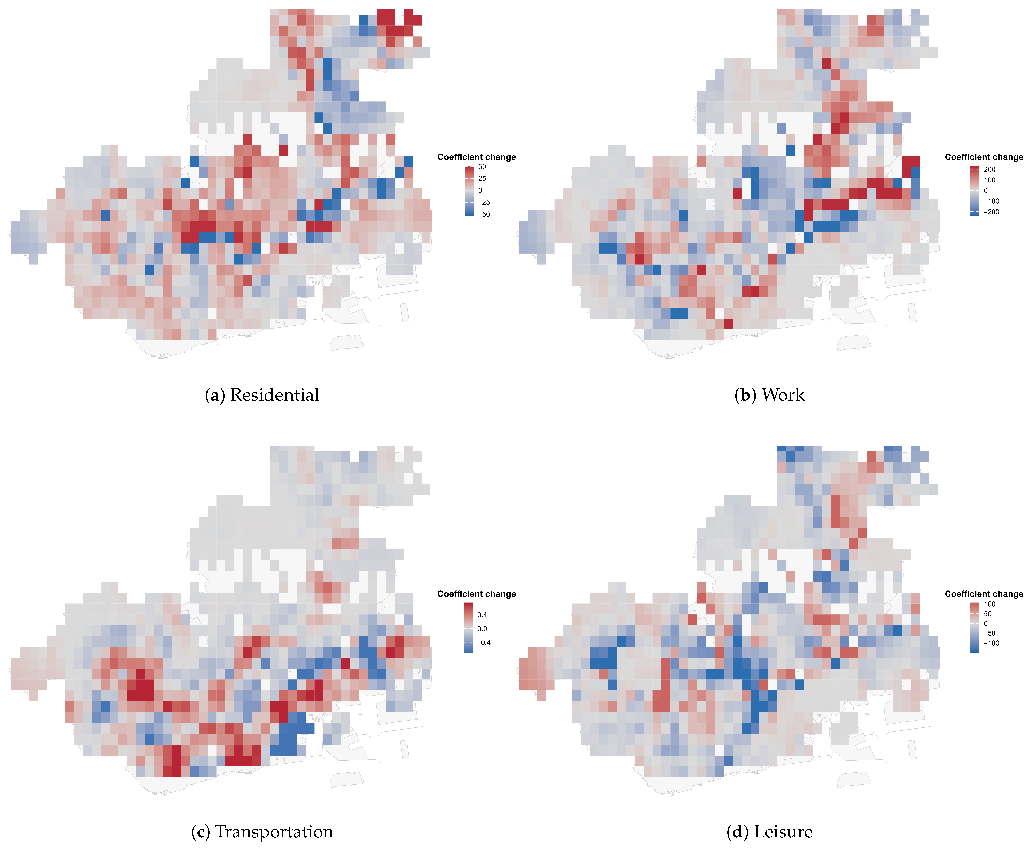
In contrast to Tokyo, we examine the changes over the same period in Kobe city, which is an important city in Japan, distinct from megacities like Tokyo and Osaka. The majority of activities and population are concentrated in the south of Kobe, and the Kita ward, namely the northern area, is predominantly residential. Figure 8 exhibits Kobe’s preference shifts. The blank areas appear on the map due to data transformation and spatial merging procedures across different years. We observe that the preference shifts are mainly located in the southern areas, whereas the changes in the northern areas are less pronounced. Though the spatial autocorrelation in preference changes is also observable in Kobe, the patterns are substantially more random and less clustered than those observed in Tokyo. For instance, zones showing considerable decreases in preference are frequently adjacent to zones of increase, and vice versa, indicating a fragmented and heterogeneous pattern.

While the preceding analysis captures general statistical patterns, taking Tokyo and Kobe as examples to show the spatial heterogeneity of preference shifts within cities, substantial variation exists across individual cities. To illustrate this heterogeneity, we present the coefficient evolution over time for six top cities in Appendix A.2, selected to represent diverse preference shifts.

4.2. Patterns of Preference Changes

The previous subsection highlighted overall shifts in amenity preferences and the spatial pattern of preference changes in Tokyo. Although we observe general preference shifts for corresponding amenity types, it is not necessary that these changes systematically co-occur. From Figure 7 and Figure 8, we can find significant spatial autocorrelation, and seemingly co-occurrence between changes in different preferences. Given such context, this section further examines the spatial patterns of these changes, focusing on the clustering of single preference changes and co-occurrence between preference changes at a more micro level.

To assess the spatial clustering of specific preference changes, Moran’s I statistics are computed for each amenity type. The index ranges from −1 to 1, where positive values indicate spatial clustering (similar values located near one another), negative values suggest dispersion (dissimilar values nearby), and values near zero imply random spatial distribution.

As shown in

Table 3. Moran’s I index of preference changes.

	2019–2020			2019–2022
	Top	Other	Full Sample	Top	Other	Full Sample
residential	0.800	0.715	0.729	0.776	0.714	0.724
work	0.741	0.708	0.714	0.744	0.715	0.720
transportation	0.719	0.735	0.732	0.734	0.771	0.765
leisure	0.790	0.703	0.718	0.759	0.716	0.723

Note: the Moran’s I statistics are estimated based on areas of city groups. The short-run and long-run are defined as the changes between 2019–2020 and 2019–2022, respectively. Source: table created by authors.

, Moran’s I values are reported separately for the top, other, and full-sample groups. The results indicate that preference changes in the top group exhibit stronger spatial clustering, especially for residential, work, and leisure amenities. In contrast, changes in preference for transportation accessibility show weaker spatial autocorrelation in the top group than in the other group.

Although the average Moran’s I values across amenity types appear similar, notable variation exists at the city level. Appendix A.3 provides examples from Tokyo and Osaka that illustrate this inter-city divergence.

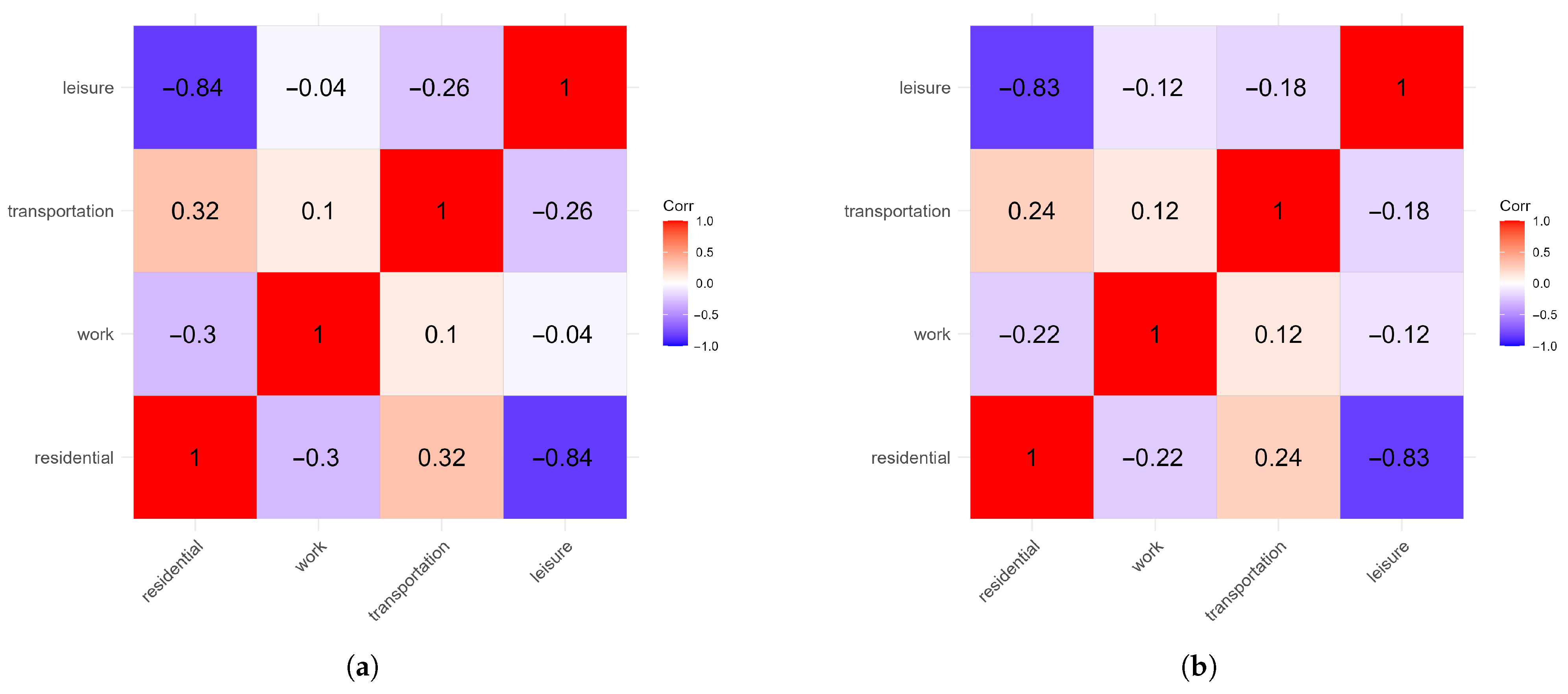
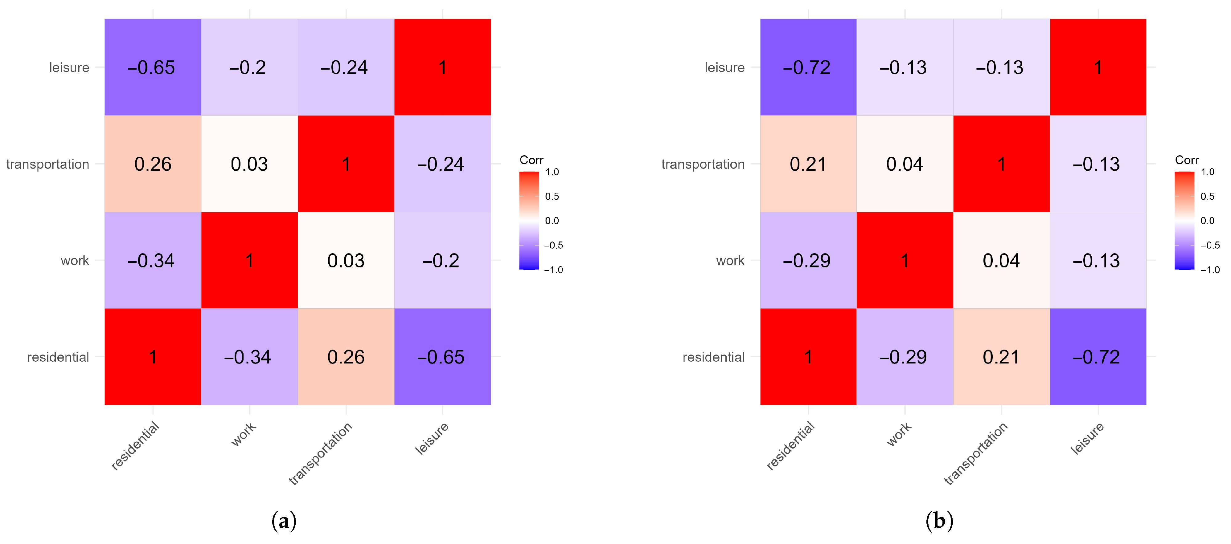
After examining spatial autocorrelation, we investigate the interdependence of preference changes using Pearson’s correlation coefficient. This metric captures linear relationships between variables, with values ranging from −1 to 1. A positive value indicates a direct correlation, while a negative value suggests an inverse relationship. The correlation matrices, presented in Figure 9 and Figure 10, are symmetrical, with diagonal entries equal to 1, reflecting perfect self-correlation. Correlations above 0.7 are considered strong, those between 0.3 and 0.7 are moderate, and values below 0.3 are weak.

In the case of the top group, three pairs of variables exhibit at least moderate correlations in the short run, all involving the residential amenity. The strongest is the negative correlation between residential and leisure, indicating that areas with increasing preference for the residential amenity tend to show declining preference for the leisure amenity. This pattern aligns with the GWR estimates. Additionally, a moderate positive correlation is observed between residential and transportation, and a moderate negative correlation is observed between residential and work. In the long run, only the negative correlation between residential and leisure remains strong, while the other associations weaken considerably.

Compared with the top group, correlations between preference dynamics in the other group are generally weaker, suggesting that preference changes occur more randomly in these cities. As shown in Figure 10, only two pairs of variables exhibit at least moderate correlations: residential and leisure, and residential and work. In the long run, the correlation between residential and work decreases slightly to 0.29, falling just below the moderate threshold, while the negative correlation between residential and leisure becomes even more pronounced.

Although our results in the previous subsection confirm substantial preference changes overall, they do not necessarily indicate that these preference changes occur in tandem. Notably, Pearson correlation coefficients reveal that preference changes in the residential amenity are closely aligned with those of other types. This pattern underscores the centrality of residential considerations in shaping urban preferences, reflecting consistent and comprehensive changes in lifestyle after the COVID-19 pandemic.

4.3. Mechanism of Preference Changes

After identifying the spatial patterns of preference changes, we next investigate the underlying mechanisms. According to the Lagrange multiplier (LM) test and the robust LM test, there is evidence of significant spatial autocorrelation in both the independent variables and the dependent variables. Therefore, we apply the SDM to account for these spatial dependencies. The model is specified as follows:

$$P{C}_i=\lambda W\times P{C}_i+\beta Amenit{y}_i+\gamma W\times Amenit{y}_i+CityF{E}_i+{ϵ}_i$$

(2)

where $P{C}_i$ denotes the post-pandemic preference change at location i for a specific amenity type, and $Amenit{y}_i$ represents the local amenity vector. The terms $W\times P{C}_i$ and $W\times Amenit{y}_i$ capture spatial lags of the dependent and independent variables, respectively. The spatial weight matrix W is constructed using the 4-nearest neighbors. Since observations from cities in the same group are estimated together, unobservable city-specific factors may exist. To control for such heterogeneity, city fixed effects $CityFE$ are included. Given that the dependent variable is derived from GWR-based preference estimates, the model is exploratory in nature. It aims to uncover correlations rather than establish causal relationships and provides insights into the spatial structure of amenity-related preference changes.

Following LeSage’s introduction [44], the coefficients in the explanatory variables can be interpreted through a decomposition framework. The direct effect reflects the influence of local variables, while the indirect effect (or spillover effect) is captured by the spatial lag terms. Furthermore, the coefficient $\lambda$ in the spatially lagged dependent variable represents residual spatial autocorrelation, often arising from omitted variables (That is, if the dependent variable is sufficiently explained by the direct and indirect effects of the independent variables, $\lambda$ should be small or statistically insignificant [45]).

From the SDM results, we focus on two key aspects: the spatial autocorrelation intensity of the preference changes and the direct and indirect effects of local amenity conditions on these changes. The estimation results are collected in

Table 4. Spatial Durbin model results: top group.

	Residential	Work	Transportation	Leisure
Intercept	−0.639 ***	0.231	−0.156 *	4.022 ***
resi19	−0.125 ***	−0.744 ***	−0.002	0.299 ***
work19	0.014 **	−0.348 ***	−0.000	0.062 ***
trans19	0.427 *	0.825	−0.039 *	−1.464
leisure19	0.080 ***	0.007	−0.000	−0.484 ***
lag_resi19	0.160 ***	0.738 ***	0.003 *	−0.466 ***
lag_work19	−0.012 *	0.365 ***	0.000	−0.101 ***
lag_trans19	−0.469 *	−0.813	0.041 *	1.767 *
lag_leisure19	−0.076 ***	−0.039	0.000	0.434 ***
$\lambda$	0.896 ***	0.692 ***	1.192 ***	0.511 ***

Note: significance levels: * $p<0.1$, ** $p<0.05$, *** $p<0.01$. Source: data from SDM estimates, and table created by authors.

and

Table 5. Spatial Durbin model estimates: other group.

	Residential	Work	Transportation	Leisure
Intercept	7.453 ***	−16.486 ***	0.001	−12.465 ***
resi19	−0.548 ***	0.250 ***	−0.000	−0.124 ***
work19	−0.001	−0.627 ***	0.000	−0.004
trans19	0.830	−8.185 **	−0.360 ***	3.855 **
leisure19	0.027 ***	0.104 ***	0.000	−0.631 ***
lag_resi19	0.538 ***	−0.055	−0.000	0.105 ***
lag_work19	0.009 **	0.579 ***	−0.000 *	−0.007
lag_trans19	−1.041	12.200 ***	0.364 ***	−3.948 **
lag_leisure19	−0.013 *	−0.146 ***	−0.000	0.568 ***
$\lambda$	0.551 ***	0.050	0.763 ***	0.525 ***

Note: significance levels: * $p<0.1$, ** $p<0.05$, *** $p<0.01$. Source: data from SDM estimates, and table created by authors.

.

Consistently positive spatial autocorrelation appears across all estimates. Moreover, the estimated $\lambda$ values are systematically higher in the top cities than in the other cities. This suggests stronger unobserved spatial linkages in large urban regions. Such latent factors likely reflect the complexity of urban systems in top-tier cities, including denser infrastructure networks and more intricate socioeconomic interdependencies. Given these dynamics, the explanatory power of observable amenity indicators may be limited, with the residual spatial patterns captured by $\lambda$. In contrast, the urban structure of smaller cities tends to be less complex, making the role of observed amenities more suitable for explaining preference changes. As a result, the spatial autocorrelation that cannot be explained by the model is generally weaker in the other group.

Regarding the coefficients of amenity variables, we observe a consistent pattern across both amenity types and city groups: the local amenity is negatively associated with corresponding preference changes while the surrounding amenity is positively correlated. This result can be explained by the mechanism of saturation, whereby the marginal utility of an amenity declines as its local concentration increases; that is, residents in already amenity-rich locations may not perceive additional value, whereas those in amenity-scarce areas gain more.

Conversely, the positive coefficients in surrounding amenities suggest a spatial spillover effect: areas adjacent to amenity-rich zones tend to experience stronger increases in preference over time. This reflects the benefits of amenity proximity: residents in nearby areas enjoy access to amenities without bearing the full burden of congestion, noise, or other associated costs (Current studies suggest that local amenities and accessibility do not always lead to stronger preferences [46], and that the costs of rich amenities, such as congestion and noise, can sometimes reduce residential attractiveness [47]).

Furthermore, we find that the magnitudes of both local and neighboring coefficients are larger in the other group. This suggests that amenity distribution has a greater influence on preference changes in smaller cities. Two factors may explain this pattern. First, as noted previously, top-tier cities possess richer amenity resources, which likely lead to saturation effects, reflected in the smaller coefficients. Second, recognizing that coefficient magnitude does not necessarily imply explanatory power, this finding is consistent with the larger $\lambda$ values observed in the top group. In contrast, preference changes in the other group are more effectively explained by both local and surrounding amenity conditions.

In summary, the SDM analysis reveals several important insights. First, spatial autocorrelation remains significant, particularly in top cities, where unobserved spatial structures appear more complex. Second, consistent local saturation and positive spillover effects are observed in both city groups, while the coefficients of both local and spillover effects in other cities show a larger magnitude. These findings underscore the heterogeneous nature of preference evolution and emphasize that the complex social and economic connections in top cities make preference changes more unpredictable.

5. Discussion

Our results reveal two major aspects of post-pandemic urban transformation in Japan: the overall direction of preference shifts and the heterogeneous shifts across cities. The overall preference shifts point to a more life-focused lifestyle, with increased demand for residential amenity and reduced importance of work-related and transportation amenity. There have been studies conducted that capture life portraits in Japan after the pandemic. For instance, Komaki et al. report that households relocated from the Tokyo and Osaka metropolitan areas in search of better educational access and higher quality of life [48], and Aoki et al., using a nationwide survey conducted in 2022, show that time saved through remote work is largely reallocated to household and leisure activities [49]. Our study provides incremental evidence from a preference-based perspective, but one of our main concerns is how the preference shifts diversify across cities.

The comparisons between top and other cities highlight two important dimensions. First, both groups display similar directional changes in residential preference, but the magnitude is substantially greater in top cities, reflecting their greater structural flexibility. Second, the patterns substantially vary in the other three amenity domains. While resource abundance in top cities partly explains these gaps, relative scarcity offers an additional rationale. Table 2 shows that the residential amenity is comparatively abundant, with a top–other ratio of about 2.5—the lowest among the four functions. In contrast, the ratios reach 3.3 for leisure and 3.5 for work, and the average distance for accessing transport in other cities is 2.7 times that of the top group. These disparities indicate that non-residential amenity is relatively scarce in other cities, which magnifies the rigidity of their preference shifts, producing sharper divergences than in the residential domain.

Additionally, we argue that differences in the prevalence of remote work also contribute to the divergence between top and other cities. Monte et al. argue that achieving a high remote work equilibrium requires a sufficiently high population and robust ICT infrastructure [15]. These conditions are readily met in top cities, enabling them not only to adopt remote work widely during the pandemic but also to sustain it afterward. By contrast, there are predominantly non-remote field works in other cities. In addition, the population size in these cities is smaller, and the ICT infrastructure is limited, which makes remote work adoption less prevalent at both the beginning and after the end of the pandemic, resulting in the preference shifts being less volatile compared with top cities.

Given the heterogeneous patterns of preference shifts observed during the study period, several policy-relevant insights emerge. First, the intensive preference changes in top-tier cities highlight the importance that governments, firms, and individuals alike must adapt to evolving lifestyle demands. Urban planners may prioritize suburban residential zones that combine high-quality amenities with accessible transportation infrastructure, thereby enhancing housing affordability while accommodating decentralized living patterns. Firms may reconsider transit from traditional office-centered models to smaller, more distributed workplaces located closer to residential clusters, supported by flexible working arrangements. At the individual level, homebuyers may increasingly seek dwellings with enhanced work-related features, such as dedicated workspaces, improved sound insulation, and reliable internet connectivity.

While providing extensive infrastructure and developing new residential zones may be feasible for megacities, these are not universal solutions, particularly for smaller cities, and Japan’s long-term depopulation is a pressing concern. A growing number of Japanese municipalities face risks of population loss (according to article published on 20 August 2024 by Population Strategy Council (Jinko Senryaku Kaigi), 744 municipalities were identified as at risk of disappearance as of 2024, although this figure has declined from 896 in 2014; see https://jichitai.works/article/details/2619), and investments in excessive infrastructure may yield limited returns.

For instance, while metropolitan areas such as Tokyo and Osaka continue to attract in-migration, many cities in Shikoku and Hokkaido face severe demographic pressures. These smaller cities face the challenge of urban shrinkage driven by depopulation. Given this context, scholars and urban planners have proposed an alternative planning strategy that acknowledges population decline and seeks to design cities capable of maintaining a high quality of life under the shrinkage—commonly referred to as “smart shrinkage”. However, Ortiz-Moya and Sieloff [50] note that some urban planners in these small cities still attempt to pursue growth-oriented development, overlooking the demographic realities of population decline. In such contexts, it may be more effective to emphasize the development of “smart” urban services, such as e-government portals, telemedicine, drone-based logistics, and elderly-oriented digital support, that can enhance accessibility and quality of life without relying on population growth. Rather than attempting to reverse urban contraction, such strategies recognize demographic realities while fostering inclusive and resilient service provision.

6. Conclusions

Employing multiple reliable data resources and using a traditional four-urban-function framework, this study examines the preference shifts and heterogeneity between different cities. Our results suggest a more life-focused lifestyle emerging in Japanese cities following the COVID-19 pandemic, while the patterns vary between top-tier and other cities.

Importantly, the observed divergence between large and small cities underscores deeper spatial asymmetries in lifestyle adaptability. Megacities, supported by institutional robustness, infrastructural depth, and occupational flexibility, are more capable of internalizing remote work, while smaller municipalities, often constrained by demographic decline and limited digital infrastructure, face greater difficulty in sustaining new urban patterns. These insights contribute to broader discussions on urban resilience, highlighting the differentiated ability of cities to absorb exogenous shocks and translate them into durable spatial reconfigurations.

From a policy standpoint, the findings caution against a uniform approach to post-pandemic urban planning. While some metropolitan areas may require zoning reforms and investment strategies that accommodate persistent hybrid work arrangements, smaller cities may benefit more from targeted support in digital infrastructure, service accessibility, and demographic adaptation. Particularly in regions experiencing population contraction, the goal may not be growth but rather the construction of sustainable, inclusive, and compact urban systems aligned with current demographic realities.

Finally, we highlight several limitations in the present study. The analysis is constrained by data availability, with observations extending only through 2022. As pandemic-related behavioral shifts may evolve further in the following years, future research should seek to validate these patterns using recent datasets. Moreover, the analysis model employed, while tractable and consistent with the prior literature, may be expanded to include other variables, such as floor–area ratio, geographical variables, and some life-related variables such as noise and air quality. Integrating disaggregated household-level preference data and exploring cross-national comparisons would also enhance the understanding of how global shocks reshape urban life across diverse contexts.