Abstract
Land-use and land-cover change detection is critical for monitoring deforestation and urban expansion. In this study, we propose an unsupervised change detection approach that leverages multi-temporal satellite imagery combined with a classic machine learning algorithm trained on automatically generated pseudo-labels. Four distinct study areas were analyzed: a tropical forest region in the Brazilian Amazon, an agricultural frontier in the Amazon, a Brazilian Savanna area undergoing transformation, and a rapidly expanding urban zone around the new Istanbul Airport, in Türkiye. The performance of the proposed approach was evaluated and compared with modern unsupervised change detection methods, including the Wavelet Energy Correlation Screening and the Temporal Convolutional Autoencoder methods. The results demonstrate that the proposed framework achieved consistently high accuracy across all four study areas, with F1-scores of approximately 0.92 in dense forest, 0.87 in an agricultural frontier, 0.91 in the savanna area, and 0.89 in an urban expansion zone. Overall, the model outperformed or matched the performance of the baseline methods, attesting to its adaptability and generalization capability in diverse environmental contexts worldwide.
1. Introduction
Land-use and land-cover (LULC) changes are one of the main current environmental challenges, with significant impacts on biodiversity, climate, and water resources. In the Legal Amazon, for example, deforestation and other anthropogenic activities have altered extensive areas of tropical forest over the past decades [1,2,3]. These transformations include both large deforestation fronts and diffuse degradation due to selective logging and illegal fires, whose cumulative effects are concerning [4,5]. Similar dynamics are observed in other parts of the world. For instance, recent studies in Türkiye have evidenced significant transitions between forest, agricultural, and urban areas in recent decades [6].
The accurate and timely detection of LULC changes through remote sensing is essential to support urban planning, environmental conservation, and sustainable land management [7,8,9]. These applications rely on change detection techniques, which identify significant alterations in a target area over time. The change detection process can be carried out according to the supervised and unsupervised learning paradigms. Unlike supervised approaches, which require labeled data for training classifiers, unsupervised methods eliminate this need and instead provide scalable cost-effective solutions for monitoring land surface dynamics using multitemporal satellite imagery. Modern unsupervised change detection frameworks can be categorized into four main groups: clustering-based algorithms, spectral transformations, deep learning models, and multivariate statistical approaches.
Considering the clustering-based branch, algorithms such as K-Means and Fuzzy C-Means remain widely used for segmenting different images. For instance, Lei et al. [10] introduced a K-Means-enhanced multi-index bitemporal framework, while Wu et al. [11] incorporated Fuzzy C-Means into dual-attention networks, underscoring their ongoing relevance in both classical and deep learning settings.
As spectral transformation approaches, the Change Vector Analysis (CVA), Principal Component Analysis (PCA), and Alternating Sequential Filtering (ASF) reduce dimensionality while isolating spectral variation. Their simplicity and efficiency make them valuable, particularly when enhanced by multiscale fusion and denoising techniques [12].
The Hotelling–Lawley Trace (HLT), as a multivariate statistical model, has emerged as a robust tool for detecting changes in high-dimensional covariance structures. Xu et al. [13] paired HLT with graph convolutional networks for PolSAR analysis, while Simpson et al. [14] validated its advantage over Likelihood Ratio Tests (LRTs). Wavelets and correlation measures have also been employed to identify temporal changes. Among such approaches, Fonseca et al. [15] proposed the Wavelet Energy Correlation Screening (WECS) technique, which emerges as an accurate and versatile method that operates over long time series of satellite images.
From a deep learning perspective, Convolutional Autoencoders and Convolutional Neural Networks (CNNs) offer unsupervised feature learning from image pairs. Recent advances have further demonstrated that deep neural networks can support very fine spatial resolution urban land cover mapping through sub-pixel mapping architectures based on learnable spatial correlation, while also enabling the annual generation of high-resolution land cover products across dozens of metropolitan areas [16,17]. These contributions extend the capability of remote sensing models to handle both high spatial detail and rich temporal dynamics in complex urban environments. Seydi et al. [18] demonstrated that multidimensional CNNs can outperform conventional pixel-based methods in LULC change detection, especially for very high-resolution images. Kalinicheva et al. [19] propose a Temporal Convolutional Autoencoder (TCAE)–based change detection framework that, in an unsupervised manner, identifies altered regions by applying thresholding to the reconstruction errors produced by Convolutional Autoencoders when processing remotely sensed image series. However, deep learning models often face computational constraints, requiring appropriate tuning to prevent overfitting. Furthermore, the use of computationally expensive models may limit their practical applicability in scenarios with limited computational resources [20,21]. Therefore, there is a need to develop change detection methods that are computationally light, efficient, and do not require advanced procedures or extensive processing resources [22].
In addition to computational and resource constraints, many existing methods also suffer from methodological limitations. With few exceptions, such as the WECS and TCAE methods, they are based on bi-temporal comparisons that consider only two points in time (before and after), limiting their capacity to capture gradual or complex temporal dynamics. Although existing techniques can perform well under various specific circumstances, they may not adequately capture the continuous temporal dynamics of changes, being susceptible to noise and seasonal variations [23,24,25,26]. To address these issues, time series-based approaches have proven effective, leveraging complete sequences of satellite imagery to capture patterns and trends over extended periods [15].
Despite these challenges, unsupervised and semi-automated machine learning techniques present a promising solution by significantly reducing the dependency on large volumes of manually labeled training data, making them more scalable and efficient. One such strategy is pseudo-labeling, which uses automatically inferred labels to train machine learning models, reducing both the effort and processing time [27,28]. In practice, the model first identifies patterns based on predefined criteria and assigns “change” or “non-change” labels to pixels without any human supervision. These pseudo-labels are then used to train a classifier, which subsequently refines the change detection process. The combination of pseudo-labeling with simple classification algorithms can result in efficient and effective models for change detection.
In response to the above-discussed issues while enhancing the adaptability of the change detection task, this study proposes an unsupervised change detection approach based on a straightforward, yet effective, machine learning algorithm, trained with pseudo-labeled examples through thresholding deviation values observed in the input data series. The methodology designed was applied to three distinct areas in Brazil and one in Türkiye. The areas in Brazil cover two regions in the Legal Amazon and another within the Brazilian Savanna biome. The area in Türkiye comprises an Istanbul region that was a scenario of intense modification due to an airport construction. The data used as part of our experiments consist of a time series of spectral indices extracted from images acquired by the Operational Land Imager (OLI) sensor onboard the Landsat-8 satellite between July 2019 and December 2020 for the first two areas, between March and September 2023 for the third area, and between July 2014 and April 2016 for the fourth area.
In summary, the main contributions of this study are as follows:
- The development of a fully unsupervised change detection methodology, based on data classification and pseudo-labels, capable of effectively detecting LULC changes using multitemporal satellite imagery.
- The successful deployment of the model across diverse global regions underscores its effectiveness in monitoring the dynamic nature of LULC changes.
- The design of a framework entirely based on statistical measures and a simple machine learning classifier, facilitating large-scale environmental monitoring without the need for extensive computational resources.
This document is structured as follows. In Section 2, we propose our unsupervised approach for detecting LULC changes. Section 3 provides details on the experiments, including the study areas, datasets, and experimental design. Section 4 presents the results obtained, followed by the corresponding discussion in Section 5. Finally, Section 6 concludes the study by highlighting the main contributions and suggesting directions for future work.
2. Unsupervised Change Detection via Pseudo-Labeling and Machine Learning Classification
The proposed approach employs an unsupervised change detection model that leverages pseudo-labeling techniques to identify land-cover changes in spectral index time series. Unlike traditional methods that rely on labeled datasets, our model generates pseudo-labels directly from the data, utilizing inherent patterns and temporal variations to infer changes without any human annotations [29]. This strategy aligns with recent advancements in remote sensing, where unsupervised models have demonstrated efficacy in detecting changes across diverse landscapes, including forested and urban areas [30]. By eliminating the need for labeled data, our approach offers a scalable solution for monitoring land-use and land-cover changes, particularly in regions where labeled datasets are scarce or unavailable.
Figure 1 illustrates the general framework of our methodology. Initially, it receives a series of images with spectral indices as input data. The images comprise the same region and are defined on the same support (i.e., the same number of columns and rows). For a given position (i.e., pixel) , we denote as the value , representing a selected spectral index of interest for .
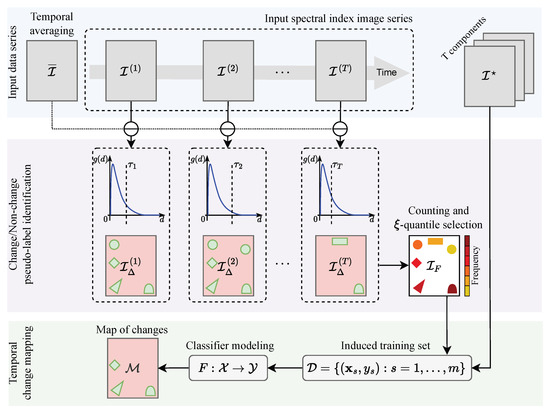
Figure 1.
Framework of the proposed unsupervised change detection method.
Considering the chronological sequence in which the images were recorded, we define the image , where , as elements of the attribute space . Furthermore, we compute a temporal average at all positions . Based on these elements, we define the absolute deviation image series as , for , where represents the deviation observed at position s and time ℓ.
For each time ℓ, values observed in are categorized as low or high deviation based on a threshold . More specifically, using the distribution of deviations represented in , we apply the method proposed by Negri and Frery [31] to determine . This method is well-suited for positive and heavy-tailed distributions like . Further details can be found in the reference cited.
Regarding the thresholding process, a location s that experiences a change at time ℓ typically exhibits a deviation value greater than . The combination of the threshold outcomes results in the image , which indicates the frequency of high deviations observed at each position s.
Formally, we have , where
Based on , positions s in the upper quantile are classified as “change” examples, while positions in the lower quantile are classified as “non-change” examples. The distinction between “change” and “non-change” is represented by the class indicator , with values of 0 and 1, respectively. The choice of should be made carefully, since small values render the selection criterion overly permissive, allowing locations with few observations to be mislabeled as “change” examples. This contamination can severely degrade classifier training (as discussed below) and, consequently, lead to unreliable results.
Consequently, based on the pseudo-labeling process discussed, we define the training set . By employing this training dataset, a classifier is modeled and applied to in order to produce a map that distinguishes changes () from non-changes ().
The Maximum Likelihood Classifier (MLC) is a computationally efficient and parameter-free classification approach that has demonstrated strong generalization capability and accurate performance across various remote sensing applications [32,33,34,35]. Additionally, because MLC requires no hyperparameter tuning, a step that must be performed carefully for alternative classifiers such as Random Forest [36] and Support Vector Machine [37], it is particularly attractive and convenient for the fully automatic context of the proposed approach. Compared to other parameter-free alternatives, such as Gaussian Naïve Bayes, preliminary experiments showed that MLC achieves higher accuracy. According to the MLC method, assuming that represents the probability distribution of class , for , estimated from , the following rule is applied to classify the pattern at position s in , thereby assigning a class label at :
In the context of the proposed approach, the classification is restricted to two classes: “non-change” () and “change” (). The class labels observed in are used to estimate the corresponding class distributions.
Despite the advantages outlined above, it is important to recognize that MLC relies on the assumption that the input data follow a specific probabilistic distribution, typically a multivariate Gaussian, owing to its flexibility in modeling generic multi-dimensional datasets. As a result, when the actual data deviate significantly from this assumption, classification performance may be adversely affected. Nevertheless, in the context of the proposed method, where the data are inherently multi-dimensional and multi-spectral-derived, the multivariate Gaussian model offers a practical and effective approximation.
Regarding the model’s behavior in the presence of subtle or gradual changes, both situations are typically labeled as “change” because they induce deviations that persist across subsequent time steps. For a subtle disturbance occurring at time t, pronounced deviations generally appear in for all ℓ ; consequently, the frequency image accumulates approximately counts in the affected region. Likewise, for a gradual land-cover transition, once deviations become consistently detectable from t onward (as indicated by thresholding ), aggregates counts across the subsequent time steps. By contrast, seasonal oscillations may sporadically trigger high deviations but do not persist; as a result, remains comparatively low, preventing seasonality from being misclassified as change.
3. Experimental Setup
3.1. Study Areas
The experiments were carried out in four distinct areas, which included two regions within the Brazilian Legal Amazon, one within the Brazilian Savanna biome, and one in northwestern Türkiye. These areas experience different types and intensities of anthropogenic pressures leading to substantial LULC changes. The selection of these geographically and environmentally contrasting regions enables the analysis of a broad spectrum of land cover transformation processes, from forest degradation and agricultural expansion to large-scale urban development. The locations of the study areas are shown in Figure 2.
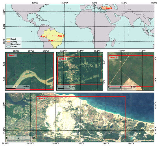
Figure 2.
Study area locations. Images acquired by the Landsat-8 OLI sensor and represented in natural color composition for Areas 1 (11 November 2020), 2 (14 October 2020), 3 (12 March 2023), and 4 (17 April 2016).
The first study area (Area 1) comprises the banks of the Madeira River in the municipality of Borba, located in the south-central portion of the state of Amazonas, Brazil. Borba is primarily accessible by river and features a mosaic of floodplain and upland forest ecosystems [38]. The region experiences a humid tropical climate with an average annual precipitation of approximately 2000 , concentrated between December and May [39]. Due to its rich biodiversity and the ecological services provided by its aquatic systems, the area holds significant environmental importance [40]. In recent decades, Borba has faced mounting environmental pressure from logging, mining, and infrastructure projects such as hydroelectric dams along the Madeira River [41]. These developments have caused deforestation, altered hydrological regimes, and led to the degradation of aquatic habitats [42], while also threatening traditional livelihoods of local and Indigenous communities [43].
The second study area (Area 2) is located in the municipality of Novo Progresso, in southwestern Pará State, Brazil. It is one of the most active deforestation frontiers in the Brazilian Amazon [44]. Driven primarily by the expansion of soybean farming and extensive cattle ranching, this region has experienced accelerated conversion of native forest into cropland and pasture [45]. Novo Progresso is situated along the BR-163 (Cuiabá–Santarém highway), whose paving has significantly increased accessibility and intensified land speculation and agricultural development [46]. The local climate is humid tropical, with rainfall averaging 2000 annually and a pronounced wet season from December to May [40]. The original vegetation consists of dense rainforest, but the region has become increasingly fragmented due to land-use change [47].
The third study area (Area 3) is located in the municipality of Cotegipe, in western Bahia State, within the Brazilian Savanna (Cerrado) biome, a region of high biodiversity currently under intense land-use pressure [48]. The expansion of soybean, cotton, and maize cultivation has accelerated the conversion of native vegetation into cropland and pasture [49,50]. The dominant land-use transition involves the suppression of native woody vegetation through burning, followed by rapid conversion to mechanized agriculture, a pattern consistent with documented uses of anthropogenic fire as a clearing tool in the Cerrado [51]. Climatically, the area has a tropical savanna (Aw) regime with pronounced wet–dry seasonality, which influences both fire dynamics and cropping calendars, further reinforcing the frontier dynamics that drive high-intensity land-use change [52].
The fourth study area (Area 4) is located in the region surrounding Istanbul Airport, in northwestern Türkiye, near the Black Sea. This area underwent a rapid and large-scale land cover transformation between 2015 and 2018, associated with the construction of one of the world’s largest airports. Prior to the development, the site was predominantly covered by mixed forest and wetlands, which were systematically cleared to accommodate the airport’s infrastructure, including runways, terminals, access roads, and logistical facilities [53,54]. The airport area covers more than 76.5 km2 and is part of a broader trend of urban expansion in the Istanbul metropolitan region [54]. This case provides a unique context of abrupt anthropogenic change in a non-tropical, urban-industrial setting, offering a valuable contrast to the gradual forest and agricultural transformations observed in the Amazon. Moreover, the magnitude and intensity of the land alteration make it an ideal test case for evaluating the ability of unsupervised methods to detect high-impact LULC changes in peri-urban zones.
3.2. Datasets
The experiments conducted in this study utilized images acquired by the OLI sensor onboard the Landsat-8 satellite. For Areas 1 and 2, the data covered the period from July 2019 to August 2020, while for Area 3, the analysis spanned from March to September 2023. In the case of Area 4, the period of analysis extended from July 2014 to April 2016. The considered intervals allowed for capturing the temporal variability associated with seasonal and anthropogenic changes in the study areas. The scenes were acquired from the United States Geological Survey (USGS) image catalog using the Google Earth Engine (GEE) platform [55]. The selected images were limited to a maximum of 40% cloud and shadow coverage. For these selected images, cloud/shadow regions were masked, and the resulting gaps were filled through temporal interpolation to ensure data consistency over time.
To enhance vegetation features and to detect changes in the study areas, three spectral indices were calculated: Normalized Difference Vegetation Index (NDVI) [56], Enhanced Vegetation Index (EVI) [57], and Soil Adjusted Vegetation Index (SAVI) [58]. NDVI allows for the assessment of photosynthetic activity and green vegetation density. On the other hand, EVI improves detection in areas of high vegetation density by correcting atmospheric and soil influences. Furthermore, SAVI minimizes soil influence, being useful in areas with sparse vegetation or exposed soil. It is worth mentioning that the use of time series of spectral indices enabled capturing seasonal variations and identifying trends or anomalous events associated with anthropogenic activities.
To evaluate the results, ground-truth reference samples were gathered following a thorough visual analysis of Areas 1 and 2. These samples were categorized into “non-change” and “change” areas. Additionally, the Project for Monitoring Deforestation in the Legal Amazon by Satellite (PRODES) [59] was utilized as auxiliary information during the collection of reference samples. PRODES annually maps deforestation activities in the Amazon by identifying clear-cut areas, offering authoritative data on regions that have experienced significant land-cover changes. By integrating PRODES data with our visual analysis, we were able to more accurately distinguish between “change” and “non-change” areas. Regarding Areas 3 and 4, the “change” and “non-change” examples were identified by a careful visual inspection. Figure 3 displays the spatial distribution of these reference samples.
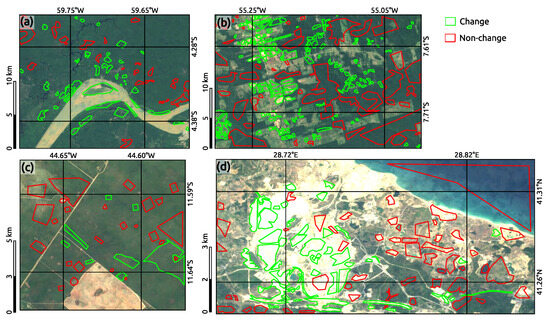
Figure 3.
Reference “change” and “non-change” samples for (a) Area 1, (b) Area 2, (c) Area 3, and (d) Area 4.
3.3. Experiment Design
The proposed methodology (Section 2) undergoes a series of experiments involving the abovementioned study areas, datasets, and reference samples discussed in Section 3.1 and Section 3.2. Specifically, these experiments utilize spectral index time series (i.e., NDVI, EVI, and SAVI) along with the quantile parameter for the analyzed areas. To ensure algorithmic simplicity, low computational cost, and good generalization ability, the MLC [60] was chosen as the classification model (i.e., , see Figure 1).
Additionally, the proposed approach was compared to the WECS and TCAE methods. The WECS method was parameterized with various wavelet families (haar, db2, db4, sym2, and sym4) and wavelet levels (1, 2, 3, 4). The TCAE approach was tested using different Convolutional Autoencoder architectures. The architectures comprise a sequence of convolutional operations followed by ReLU activations, except in the output layer where a Sigmoid activation function is employed. According to this, we denote by Arch-1 the TCAE architecture, which applies a convolutional filtering operation in the input image series to encode it and then the same operation to decode and reconstruct the original representation (i.e., in simple notation; Input–32–Output). Following the same scheme, Arch-2 applies a and a convolutional filter to decode the input image series and a filtering to decode it (i.e., in simple notation: Input–32–16–32–Output). Generalizing, Archs-3, -4, -5, and -6 consider the sequences 32–16–8–16–32, 32–16–8–4–8–16–32, and 32–16–8–4–2–4–8–16–32 for the convolutional kernel filters to encode and decode the input time series. All the architectures were trained for 200 epochs or until the loss function did not show a decrement superior to after 10 epochs. The mean squared error was adopted as the loss function, and the Adam algorithm was employed to optimize the network parameters under a learning rate of . Lastly, the reconstruction error was then used as a measure to represent spatio-temporal changes.
Both WECS and TCAE approaches transform the complete input spectral index image series into a single-band representation, where high values tend to be assigned to temporal change events. In order to segregate locations submitted to change over the analyzed period, we applied a thresholding algorithm. The tested thresholding algorithms included the Otsu [61] (OT), Kittler–Illingworth [62] (KI), Yen [63] (YE), Sauvola [64] (SA), Rosin [65] (TR), and Niblack [66] (NI).
The accuracy of the results is measured using the kappa coefficient [67] and F1-score [68]. In summary, the F1-score, defined as , is the harmonic mean of precision (Pr) and recall (Re), providing a balanced measure of the classification performance. The kappa coefficient, given by , quantifies the agreement between the predicted and actual classifications, corrected for chance. In this expression, is the observed agreement, and is the expected agreement by chance. Here, , , , and represent the counts of true positives, true negatives, false positives, and false negatives, respectively. In the specific context of change detection, the positive class corresponds to the “change” category, while the negative class refers to “non-change”. Accordingly, the “True” components ( and ) represent correctly identified pixels for both change and non-change classes, whereas the “False” components ( and ) indicate misclassifications between these two categories. The quantities , , , and are computed by comparing the classification results with the available reference samples, as illustrated in Figure 3.
The proposed method was implemented using IDL (Interactive Data Language) version 9.0, and both the source code and data are freely available at https://github.com/rogerionegri/TauTS. The cartographic representations and charts presented in the following sections were produced using QGIS 3.40 [69] and the Matplotlib 3.10 library for Python 3.12 [70], respectively.
4. Results
Following the experimental design outlined in Section 3.3, an extensive set of results was obtained. Table 1 presents the best outcomes achieved by each method across the different study areas and the respective run times in seconds. A detailed overview of the experiments is provided in Figure 4, Figure 5, Figure 6, Figure 7, Figure 8, Figure 9, Figure 10, Figure 11, Figure 12 and Figure 13, which illustrate the accuracy values obtained for various input datasets and parameter configurations. The results highlighted in Table 1 are also depicted in Figure 14, Figure 15, Figure 16 and Figure 17, which show the corresponding change detection maps.

Table 1.
Summary of the best results delivered by the analyzed methods according to F1-score and kappa coefficient. SI, WF, L, , and Arch stand for spectral index, wavelet family, level, thresholding algorithm, and the neural network architecture, respectively.
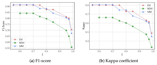
Figure 4.
Proposed method performance in Area 1 under different setups.
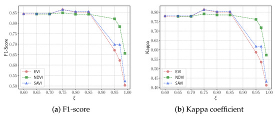
Figure 5.
Proposed method performance in Area 2 under different setups.
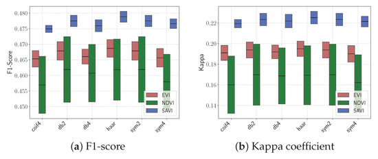
Figure 6.
Performance of WECS in Area 2. Range bars represent variation across decomposition levels and thresholding methods.
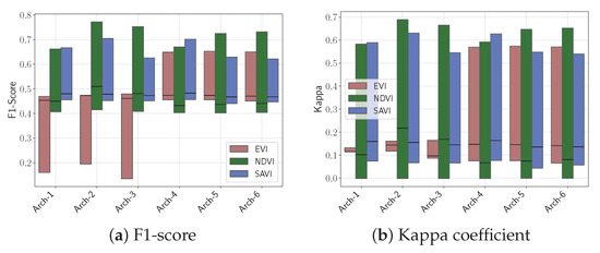
Figure 7.
Performance of TCAE in Area 2. Range bars represent variation across thresholding methods.
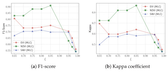
Figure 8.
Proposed method performance in Area 3 under different setups.
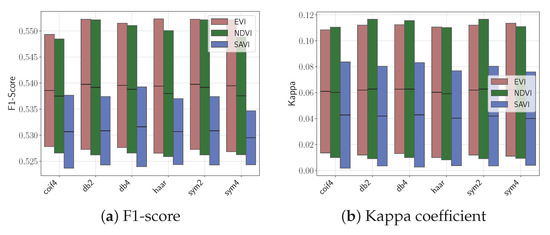
Figure 9.
Performance of WECS in Area 3. Range bars represent variation across decomposition levels and thresholding methods.
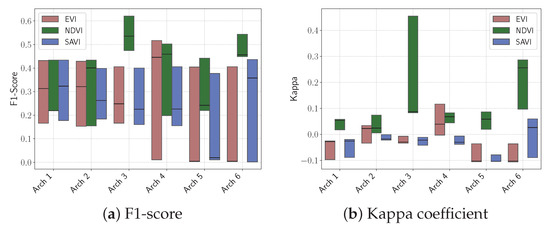
Figure 10.
Performance of TCAE in Area 3. Range bars represent variation across thresholding methods.
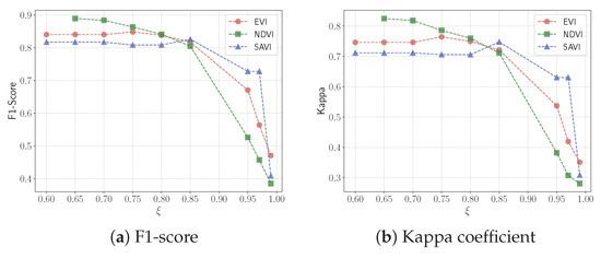
Figure 11.
Proposed method performance in Area 4 under different setups.
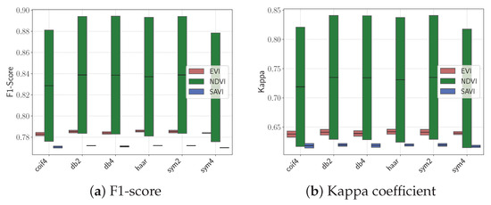
Figure 12.
Performance of WECS in Area 4. Range bars represent variation across decomposition levels and thresholding methods.
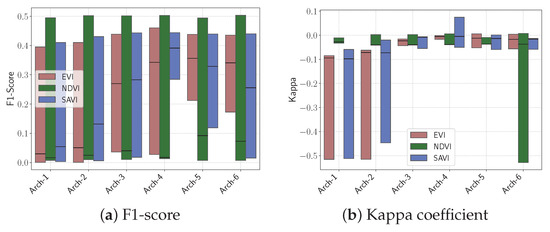
Figure 13.
Performance of TCAE in Area 4. Range bars represent variation across thresholding methods.
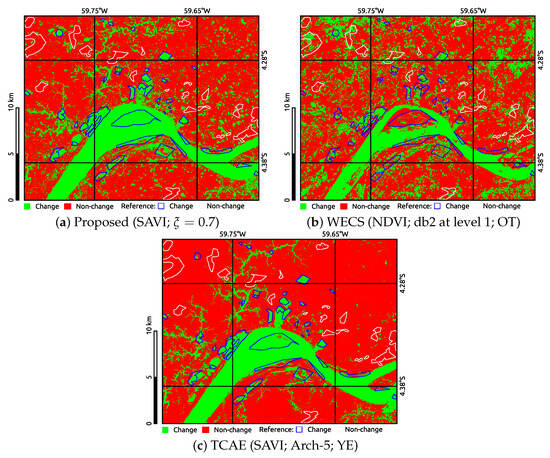
Figure 14.
Best change/non-change maps for Area 1.
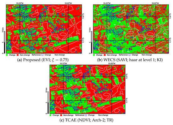
Figure 15.
Best change/non-change maps for Area 2.
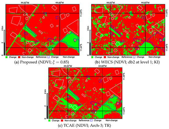
Figure 16.
Best change/non-change maps for Area 3.
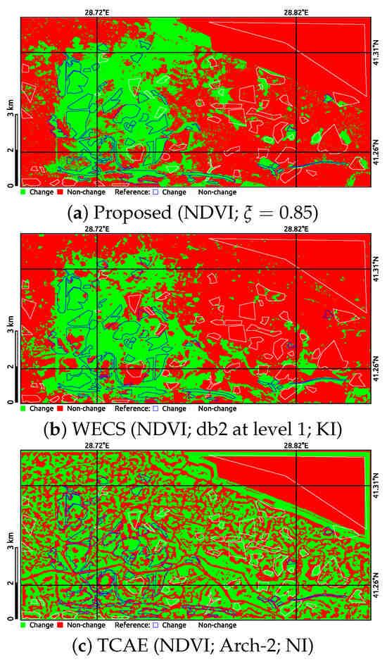
Figure 17.
Best change/non-change maps for Area 4.
Regarding the results for Area 1, one may observe that the proposed method using the SAVI index at achieved the best performance, with an F1-score of 0.92 and a kappa coefficient of 0.81. The EVI index also performed well, though slightly lower than SAVI. Additionally, it may be observed that as the threshold increased, both metrics decreased across all indices (Figure 4). Furthermore, the proposed methodology could not be executed with upper quantile for NDVI or with for EVI and SAVI. This limitation arises from the inability to identify sufficient “pseudo-labeled change” examples at those values. By contrast, the best result obtained by the WECS method in Area 1 was with the NDVI index using the db2 wavelet family at level 1 and Otsu’s algorithm for thresholding, resulting in an F1-score of 0.75 and kappa of 0.45 (Figure 18). Regarding the TCAE results, the highest accuracy was obtained using the SAVI index combined with Yen’s thresholding algorithm and Arch-5. This configuration achieved an impressive F1-score of 0.99 and a kappa coefficient of 0.83. Arch-5 represents one of the most complex architectures among those tested, consisting of five convolutional layers in both the encoder and decoder stages (Figure 19). Although the TCAE approach yielded slightly higher accuracy metrics compared to our proposed method in specific configurations, both methods substantially outperformed the WECS baseline across the considered study area.
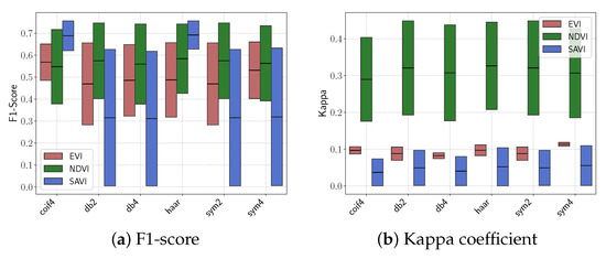
Figure 18.
Performance of WECS in Area 1. Range bars represent variation across decomposition levels and thresholding methods.
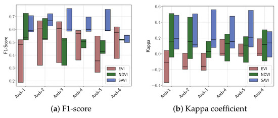
Figure 19.
Performance of TCAE in Area 1. Range bars represent variation across thresholding methods.
With respect to Area 2, a region characterized by intense agricultural activity, the proposed model again achieved the best results using the EVI index at = 0.75. This configuration resulted in an F1-score of 0.87 and a kappa coefficient of 0.81 (Figure 5). As in Area 1, increasing led to decreases in both metrics. Moreover, the method could not be executed with for NDVI or with for EVI and SAVI. In addition, the SAVI index also performed very close to the EVI index. The best result achieved by the WECS method in Area 2 was obtained using the SAVI index with the haar wavelet family at level 1 and Kittler–Illingworth thresholding algorithm, yielding an F1-score of 0.48 and a kappa of 0.23, which is significantly lower than the proposed model’s performance (Figure 6). Concerning the TCAE method, the highest accuracy in Area 2 was achieved using the NDVI index with Arch-2 (i.e., the second-simplest architecture evaluated), combined with the Triangle thresholding algorithm. While this configuration outperformed the WECS baseline, it remained inferior to the proposed method (Figure 7).
In the case of Area 3, a region experiencing significant land-use pressure due to the conversion of native woodlands into agricultural areas through cutting and burning, the proposed method achieved its best performance using the NDVI index with , resulting in an F1-score of 0.91 and a kappa coefficient of 0.86 (Figure 8). In contrast, the WECS method performed very poorly in this area, with F1-scores around 0.5 and kappa values close to 0.1, even when using the best-performing inputs such as the NDVI and EVI indices (Figure 9). The TCAE method produced results inferior to the proposed approach, achieving an F1-score of 0.66 and a kappa coefficient of 0.49 when configured with the Arch-3 architecture and the Triangle thresholding algorithm (Figure 10).
Concerning Area 4, a large-scale urban development project, both the proposed and WECS methods performed well and achieved similar accuracy values. The best performance for the proposed model using NDVI at = 0.65 was an F1-score of 0.89 and a kappa coefficient of 0.82 (Figure 8). The WECS method, using the NDVI index with the db2 wavelet family at level 1 and Kittler–Illingworth thresholding, achieved an impressive F1-Score of 0.89 and kappa of 0.84 (Figure 9). Conversely, the TCAE approach yielded very poor results regardless of the adopted spectral index, network architecture, or thresholding algorithm (Figure 10). This suggests that, in such a complex setting, the convolutional representations learned by the model may have produced insufficiently discriminative features to separate temporal changes.
According to the results obtained with the proposed approach, the parameter plays a crucial role in the sensitivity of LULC change detection, exhibiting a consistent trend across all four study areas (Figure 4, Figure 5, Figure 8 and Figure 11). Usually, lower values of (e.g., 0.75) enhance the detection capability, resulting in higher F1-scores and kappa coefficients across all study areas. Except for Area 3, as increases, the model becomes more conservative, thereby reducing its ability to identify true positives. Conversely, excessively low values of hinder the identification of suitable examples for training the classifier, compromising the method’s effectiveness.
In light of the above discussions, the proposed model exhibited strong and consistent performance across all four study areas, effectively adapting to diverse LULC characteristics. As shown in Figure 4, Figure 5, Figure 6, Figure 7, Figure 8, Figure 9, Figure 10, Figure 11, Figure 12 and Figure 13, although it did not outperform the WECS and TCAE methods in every case in terms of kappa and F1-score, its results remained consistently high, underscoring the model’s robustness.
The computational time across the four study areas, as shown in Figure 20, indicates that the WECS method consistently achieves the lowest processing times, demonstrating superior computational efficiency. With the exception of Area 3, TCAE ranks second in performance, while the proposed method exhibits the highest computational cost in Areas 1, 2, and 4. Although the proposed approach may provide advantages in terms of accuracy and spatial consistency, it generally incurs higher processing time. Given this computational burden, future work should explore strategies to optimize and reduce the method’s execution time, particularly for large-scale applications.
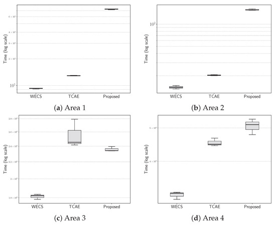
Figure 20.
Run times for the WECS, TCAE, and proposed methods across the four study areas.
Visual inspection of the change detection maps, depicted in Figure 14, Figure 15, Figure 16 and Figure 17, confirms the superior spatial precision of the proposed method. The ground reference samples representing change and non-change areas (Figure 3) were superimposed to facilitate verification. In Area 1, the proposed model successfully identified small-scale deforestation patches, with minimal false alarms. In contrast, the WECS method, while capturing the broader changes, missed smaller deforested areas and exhibited more false positives. The TCAE method produced more regularized (i.e., smoother) outputs, which is consistent with its strong performance according to the adopted accuracy metrics.
Similarly, in Area 2, the proposed method detected subtle agricultural expansion and deforestation with greater clarity and fewer spurious detections compared to WECS, which tended to overestimate changes in areas with mixed land use. The TCAE method produced results comparable to those of the proposed approach; however, due to the convolutional operations applied, the outputs became excessively smooth, which led to an increased false positive rate (i.e., detecting “changes” in areas where no changes were expected).
In Area 3, the proposed method maintained its ability to avoid overestimating the extent of change while successfully preserving narrow linear structures, a characteristic also observed in the outputs of the TCAE model. Although the TCAE method produced comparable but less consistent results, characterized by fragmented and isolated detections, it failed to capture several change regions and also committed inclusion errors, particularly in the southeastern portion of the study area. In contrast, the WECS method was unable to identify large areas subjected to land-use transformation, which helps to explain the weak quantitative performance previously reported for this method.
Lastly, in Area 4, although the WECS method achieved high accuracy, the proposed method produced cleaner and more precise maps of land-cover change, with fewer false positives and a sharper delineation of the new airport infrastructure. In contrast, the TCAE method failed to generate informative results, mainly due to the high spectral variability observed during the study period, which limited its ability to capture consistent change patterns. The greater spatial complexity of Area 4, marked by fragmented and irregular LULC transitions, further challenged TCAE, whose convolutional representations struggled to reconstruct fine structures, leading to inconsistent maps. This highlights the difficulties faced by deep learning approaches in highly heterogeneous environments without explicit supervision. Future work could address these limitations by incorporating auxiliary data sources, such as SAR imagery, or by designing feature sets better suited to structural variability.
5. Discussion
The findings of this study have significant environmental implications, particularly in the context of monitoring and managing land-use changes. The ability to accurately detect changes in LULC is crucial for understanding the extent of deforestation, assessing the impacts of agropastoral and urban expansion, and implementing effective conservation strategies [71,72].
The proposed change detection model demonstrated consistent and reliable performance across all study areas. In Area 1, which is predominantly forested with minimal agricultural activities, the model effectively identified subtle changes in vegetation cover. This capability is essential for the early detection of illegal logging and small-scale deforestation activities that may not be immediately apparent but can cumulatively lead to significant environmental degradation [73,74].
In Area 2, characterized by extensive agricultural activities and dynamic land-use changes, the model’s effectiveness in capturing rapid and significant alterations in LULC is particularly valuable. The accurate detection of changes due to the cultivation of annual crops, like soy and corn, enables better monitoring of agricultural expansion and its encroachment into forested areas [75]. This information is critical for enforcing land-use regulations and promoting sustainable agricultural practices [76]. Similarly, for Areas 3 and 4, the proposed method provided a more precise delineation of urban expansion.
The comparison among the three methods reveals distinct behaviors when applied to varying spatial patterns of land-cover change. The WECS method consistently exhibited a tendency to overestimate change, which aligns with the spatial regularization introduced by its wavelet-based processing. While this smoothing effect enhances object continuity, it also enlarges change boundaries and increases false positives, limiting the method’s ability to detect small-scale or localized transformations. In contrast, the TCAE model performed well in scenarios where changes were spatially extensive and well-defined, achieving high true positive rates. However, in areas marked by fine-grained or complex transitions, the convolutional operations, inherently aggregative and deeply iterative by design, acted similarly to, or even more strongly than, wavelets, ultimately blurring spatial detail and producing inconsistent detection outcomes.
The proposed approach differs conceptually by operating in the temporal rather than spatial domain, focusing on the evolution of each pixel’s temporal signature. This design reduces spatial smoothing and, consequently, improves the sensitivity to localized and small-scale changes. However, the method depends on the proper tuning of the threshold parameter , which defines the decision boundary between change and non-change. In summary, when changes predominantly occur at regional scales, TCAE remains competitive; WECS may also yield reasonable results but tends to overestimate the change; and the proposed method demonstrates more balanced performance, effectively capturing both localized and large-scale transformations.
From an operational perspective, the proposed technique can be seamlessly integrated into a processing pipeline that periodically ingests pre-processed spectral index time series to generate up-to-date change maps highlighting recently impacted areas. Such a pipeline could directly support large-scale monitoring initiatives, for example by complementing the PRODES program [59], where continuous deforestation detection is critical for environmental governance. By automatically updating change maps, the method could enhance the mentioned workflows, providing refined and timely insights into forest loss dynamics. Likewise, in the context of urban planning agencies, the technique could be employed to monitor land-use transitions, assess the expansion of impervious surfaces, and identify encroachment into environmentally sensitive zones. This integration would not only reduce the time between image acquisition and actionable information but also strengthen decision-making in both environmental monitoring and sustainable urban management.
6. Conclusions
This study proposed an unsupervised change-detection framework applied for long (i.e., non-binary) remote sensing image series that couples pseudo-labeling with a classic Machine Learning classification approach; specifically the Maximum Likelihood Classifier. We evaluated the approach on four contrasting regions, three in Brazil and one in Türkiye, using the EVI, SAVI, and NDVI indices computed from multispectral images acquired by the Landsat-8 OLI sensor. The results were benchmarked against two alternative approaches, the WECS and TCAE, that are formalized according to distinct concepts.
Across all study areas, the proposed model demonstrated performance that was comparable to or exceeded that of the WECS and TCAE approaches. Peak F1-scores reached 0.92 (kappa = 0.81) in a predominantly forested region, 0.87 (kappa = 0.81) in an agriculturally dynamic landscape, 0.91 (kappa = 0.86) in a savanna area under transformation, and 0.89 (kappa = 0.82) in a rapidly urbanizing area. The sensitivity analysis showed that usually moderate values (0.65∼0.75) strike the best balance between detecting subtle changes and suppressing noise, whereas higher thresholds become overly conservative.
The framework’s strong performance in both forest and urban/agropastoral contexts underscores its suitability for large-scale monitoring tasks such as deforestation surveillance, infrastructure expansion assessment, and land-use management. Because the method relies on a simple classifier with no hyperparameter tuning, it is straightforward to implement and readily transferable to operational workflows.
Potential directions for future research include the following: (i) developing an automated strategy for selecting ; (ii) evaluating the generalization capability of the proposed method across additional biomes and sensor modalities; (iii) incorporating imagery with higher temporal resolution to improve the detection of rapid disturbances; (iv) extending the analysis to other satellite sensors (e.g., Sentinel-2) and spectral indices beyond vegetation-related ones (e.g., NDBI for urban areas), in order to validate the method in broader application contexts; (v) extending the proposed method to multivariate time series, (vi) creating feature-level visualization strategies for deeper analysis of the results, and (vii) investigating advanced classification strategies, including deep learning techniques, to further enhance robustness in complex and heterogeneous environments.
Author Contributions
Conceptualization, R.G.N.; Methodology, F.M.C., A.B., A.S., E.A.d.S., G.P.C. and W.C.; Software, R.G.N., L.M.V.A. and E.A.d.S.; Validation, R.G.N., A.B., A.S., E.A.d.S. and W.C.; Formal analysis, F.M.C., L.M.V.A., A.B. and G.P.C.; Investigation, F.M.C., L.M.V.A., A.S., G.P.C. and W.C.; Writing—original draft, F.M.C., R.G.N., L.M.V.A., A.B., A.S., E.A.d.S., G.P.C. and W.C.; Project administration, R.G.N. All authors have read and agreed to the published version of the manuscript.
Funding
This research was supported by the São Paulo State University, the São Paulo Research Foundation (FAPESP), 2023/14427-8 and 2024/01610-1, and the National Council for Scientific and Technological Development (CNPq), grants 316228/2021-4 and 305220/2022-5.
Institutional Review Board Statement
Not applicable.
Informed Consent Statement
Not applicable.
Data Availability Statement
The datasets, codes, and the complete set of results are available at https://github.com/rogerionegri/TauTS.
Conflicts of Interest
The authors declare no conflicts of interest.
References
- Fearnside, P.M. Deforestation in Brazilian Amazonia: History, rates, and consequences. Conserv. Biol. 2005, 19, 680–688. [Google Scholar] [CrossRef]
- Malhi, Y.; Roberts, J.T.; Betts, R.A.; Killeen, T.J.; Li, W.; Nobre, C.A. Climate change, deforestation, and the fate of the Amazon. Science 2008, 319, 169–172. [Google Scholar] [CrossRef] [PubMed]
- Nobre, C.A.; Sampaio, G.; Borma, L.S.; Castilla-Rubio, J.C.; Silva, J.S.; Cardoso, M. Land-use and climate change risks in the Amazon and the need of a novel sustainable development paradigm. Proc. Natl. Acad. Sci. USA 2016, 113, 10759–10768. [Google Scholar] [CrossRef] [PubMed]
- Aragão, L.E.O.C.; Shimabukuro, Y.E. The incidence of fire in Amazonian forests with implications for REDD. Science 2010, 328, 1275–1278. [Google Scholar] [CrossRef] [PubMed]
- Richards, P.D.; VanWey, L. Where deforestation leads to urbanization: How resource extraction is leading to urban growth in the Brazilian Amazon. Ann. Assoc. Am. Geogr. 2015, 105, 806–823. [Google Scholar] [CrossRef]
- Aksoy, H.; Kaptan, S.; Keçecioğlu Dağli, P.; Atar, D. Unveiling two decades of forest transition in Anamur, Türkiye: A remote sensing and GIS-driven intensity analysis (2000–2020). Front. For. Glob. Change 2024, 7, 1498890. [Google Scholar] [CrossRef]
- Achard, F.; Beuchle, R.; Mayaux, P.; Stibig, H.J.; Bodart, C.; Brink, A.; Carboni, S.; Desclée, B.; Donnay, F.; Eva, H.D.; et al. Determination of tropical deforestation rates and related carbon losses from 1990 to 2010. Glob. Change Biol. 2014, 20, 2540–2554. [Google Scholar] [CrossRef]
- Hansen, M.C.; Potapov, P.V.; Goetz, S.J.; Turubanova, S.; Tyukavina, A.; Krylov, A.; Kommareddy, A.; Egorov, A. Mapping tree height distributions in Sub-Saharan Africa using Landsat 7 and 8 data. Remote Sens. Environ. 2016, 185, 221–232. [Google Scholar] [CrossRef]
- Phiri, D.; Simwanda, M.; Salekin, S.; Nyirenda, V.R.; Murayama, Y.; Ranagalage, M. Sentinel-2 Data for Land Cover/Use Mapping: A Review. Remote Sens. 2020, 12, 2291. [Google Scholar] [CrossRef]
- Lei, G.; Li, A.; Bian, J.; Naboureh, A.; Zhang, Z.; Nan, X. A Simple and Automatic Method for Detecting Large-Scale Land Cover Changes Without Training Data. IEEE J. Sel. Top. Appl. Earth Obs. Remote Sens. 2023, 16, 7276–7292. [Google Scholar] [CrossRef]
- Wu, D.; Li, M.; Wu, Y.; Zhang, P.; Xin, X. Dual Attention-Based Global-Local Feature Extraction Network for Unsupervised Change Detection in PolSAR Images. IEEE J. Sel. Top. Appl. Earth Obs. Remote Sens. 2024, 17, 10842–10861. [Google Scholar] [CrossRef]
- Colin Koeniguer, E.; Nicolas, J.M. Change Detection Based on the Coefficient of Variation in SAR Time-Series of Urban Areas. Remote Sens. 2020, 12, 2089. [Google Scholar] [CrossRef]
- Xu, D.; Li, M.; Wu, Y.; Zhang, P.; Xin, X.; Yang, Z. Difference-guided multiscale graph convolution network for unsupervised change detection in PolSAR images. Neurocomputing 2023, 555, 126611. [Google Scholar] [CrossRef]
- Simpson, M.D.; Akbari, V.; Marino, A.; Prabhu, G.N.; Bhowmik, D.; Rupavatharam, S.; Datta, A.; Kleczkowski, A.; Sujeetha, J.A.R.P.; Anantrao, G.G.; et al. Detecting Water Hyacinth Infestation in Kuttanad, India, Using Dual-Pol Sentinel-1 SAR Imagery. Remote Sens. 2022, 14, 2845. [Google Scholar] [CrossRef]
- Fonseca, R.V.; Negri, R.G.; Pinheiro, A.; Atto, A.M. Wavelet Spatio-Temporal Change Detection on Multitemporal SAR Images. IEEE J. Sel. Top. Appl. Earth Obs. Remote Sens. 2023, 16, 4013–4023. [Google Scholar] [CrossRef]
- He, D.; Shi, Q.; Xue, J.; Atkinson, P.M.; Liu, X. Very fine spatial resolution urban land cover mapping using an explicable sub-pixel mapping network based on learnable spatial correlation. Remote Sens. Environ. 2023, 299, 113884. [Google Scholar] [CrossRef]
- He, D.; Shi, Q.; Liu, X.; Zhong, Y.; Xia, G.; Zhang, L. Generating annual high resolution land cover products for 28 metropolises in China based on a deep super-resolution mapping network using Landsat imagery. GIScience Remote Sens. 2022, 59, 2036–2067. [Google Scholar] [CrossRef]
- Seydi, S.T.; Hasanlou, M.; Amani, M. A New End-to-End Multi-Dimensional CNN Framework for Land Cover/Land Use Change Detection in Multi-Source Remote Sensing Datasets. Remote Sens. 2020, 12, 2010. [Google Scholar] [CrossRef]
- Kalinicheva, E.; Sublime, J.; Trocan, M. Change Detection in Satellite Images using Reconstruction Errors of Joint Autoencoders. In Artificial Neural Networks and Machine Learning–ICANN 2019: Image Processing, Proceedings of the 28th International Conference on Artificial Neural Networks, Munich, Germany, 17–19 September 2019; Lecture Notes in Computer Science; Springer: Cham, Switzerland, 2019; pp. 637–648. [Google Scholar] [CrossRef]
- Gao, F.; Masek, J.; Schwaller, M.; Hall, F. On the blending of the Landsat and MODIS surface reflectance: predicting daily Landsat surface reflectance. IEEE Trans. Geosci. Remote Sens. 2006, 44, 2207–2218. [Google Scholar] [CrossRef]
- Zhu, Z.; Woodcock, C.E. Continuous change detection and classification of land cover using all available Landsat data. Remote Sens. Environ. 2014, 144, 152–171. [Google Scholar] [CrossRef]
- Olofsson, P.; Foody, G.M.; Herold, M.; Stehman, S.V.; Woodcock, C.E.; Wulder, M.A. Good practices for estimating area and assessing accuracy of land change. Remote Sens. Environ. 2014, 148, 42–57. [Google Scholar] [CrossRef]
- Belgiu, M.; Drăguţ, L. Random forest in remote sensing: A review of applications and future directions. ISPRS J. Photogramm. Remote Sens. 2016, 114, 24–31. [Google Scholar] [CrossRef]
- Zhu, X.; Tuia, D.; Mou, L.; Xia, G.S.; Zhang, L.; Xu, F.; Fraundorfer, F. Deep Learning in Remote Sensing: A Comprehensive Review and List of Resources. IEEE Geosci. Remote Sens. Mag. 2017, 5, 8–36. [Google Scholar] [CrossRef]
- Wu, J.S.; Fu, G. Modelling aboveground biomass using MODIS FPAR/LAI data in alpine grasslands of the Northern Tibetan Plateau. Remote Sens. Remote Sens. Lett. 2018, 9, 150–159. [Google Scholar] [CrossRef]
- Souza, C.M.; Shimbo, J.Z.; Rosa, M.R.; Parente, L.L.; Alencar, A.; Rudorff, B.F.T.; Hasenack, H.; Matsumoto, M.; Ferreira, L.G.; Souza-Filho, P.W.M.; et al. Reconstructing three decades of land use and land cover changes in Brazilian biomes with Landsat archive and earth engine. Remote Sens. 2020, 12, 2735. [Google Scholar] [CrossRef]
- Lee, D.H. Pseudo-Label: The Simple and Efficient Semi-Supervised Learning Method for Deep Neural Networks. 2013. Available online: https://www.kaggle.com/blobs/download/forum-message-attachment-files/746/pseudo_label_final.pdf (accessed on 1 October 2025).
- Negri, R.G.; Luz, A.E.O.; Frery, A.C.; Casaca, W. Mapping Burned Areas with Multitemporal–Multispectral Data and Probabilistic Unsupervised Learning. Remote Sens. 2022, 14, 5413. [Google Scholar] [CrossRef]
- Zhao, C.; Pan, Y.; Ren, S.; Gao, Y.; Wu, H.; Ma, G. Accurate vegetation destruction detection using remote sensing imagery based on the three-band difference vegetation index (TBDVI) and dual-temporal detection method. Int. J. Appl. Earth Obs. Geoinf. 2024, 127, 103669. [Google Scholar] [CrossRef]
- Zhang, B.; Wang, Z.; Du, B. Boosting Semi-Supervised Object Detection in Remote Sensing Images With Active Teaching. IEEE Geosci. Remote Sens. Lett. 2024, 21, 6003505. [Google Scholar] [CrossRef]
- Negri, R.G.; Frery, A.C. Unsupervised Change Detection Driven by Floating References: A Pattern Analysis Approach. Pattern Anal. Appl. 2021, 24, 933–949. [Google Scholar] [CrossRef]
- Liang, S.; Cheng, J.; Zhang, J. Maximum Likelihood Classification of Soil Remote Sensing Image Based on Deep Learning. Earth Sci. Res. J. 2020, 24, 357–365. [Google Scholar] [CrossRef]
- Razaque, A.; Ben Haj Frej, M.; Almi’ani, M.; Alotaibi, M.; Alotaibi, B. Improved Support Vector Machine Enabled Radial Basis Function and Linear Variants for Remote Sensing Image Classification. Sensors 2021, 21, 4431. [Google Scholar] [CrossRef]
- Sisodia, P.S.; Tiwari, V.; Kumar, A. Analysis of Supervised Maximum Likelihood Classification for remote sensing image. In Proceedings of the International Conference on Recent Advances and Innovations in Engineering (ICRAIE-2014), Jaipur, India, 9–11 May 2014; pp. 1–4. [Google Scholar] [CrossRef]
- Sisodia, P.S.; Tiwari, V.; Kumar, A. A comparative analysis of remote sensing image classification techniques. In Proceedings of the 2014 International Conference on Advances in Computing, Communications and Informatics (ICACCI), Delhi, India, 24–27 September 2014; pp. 1418–1421. [Google Scholar] [CrossRef]
- Breiman, L. Random Forests. Mach. Learn. 2001, 45, 5–32. [Google Scholar] [CrossRef]
- Cortes, C.; Vapnik, V. Support-vector networks. Mach. Learn. 1995, 20, 273–297. [Google Scholar] [CrossRef]
- Castello, L.; Macedo, M.N. Large-scale degradation of Amazonian freshwater ecosystems. Glob. Change Biol. 2016, 22, 990–1007. [Google Scholar] [CrossRef] [PubMed]
- Alvares, C.A.; Stape, J.L.; Sentelhas, P.C.; de Moraes Goncalves, J.L.; Sparovek, G. Köppen’s climate classification map for Brazil. Meteorol. Z. 2013, 22, 711–728. [Google Scholar] [CrossRef] [PubMed]
- Junk, W.J.; Piedade, M.T.F.; Schöngart, J.; Wittmann, F. A classification of major natural habitats of Amazonian white-water river floodplains (várzeas). Wetl. Ecol. Manag. 2012, 20, 461–475. [Google Scholar] [CrossRef]
- Fearnside, P.M. Impacts of Brazil’s Madeira River Dams: Unlearned lessons for hydroelectric development in Amazonia. Environ. Sci. Policy 2014, 38, 164–172. [Google Scholar] [CrossRef]
- Tundisi, J.; Goldemberg, J.; Matsumura-Tundisi, T.; Saraiva, A. How many more dams in the Amazon? Energy Policy 2014, 74, 703–708. [Google Scholar] [CrossRef]
- Fearnside, P.M. Hydroelectric Dams in the Brazilian Amazon as Sources of ‘Greenhouse’ Gases. Environ. Conserv. 1995, 22, 7–19. [Google Scholar] [CrossRef]
- Fearnside, P. Deforestation of the Brazilian Amazon. In Oxford Research Encyclopedia of Environmental Science; Oxford University Press: Oxford, UK, 2017. [Google Scholar] [CrossRef]
- Barona, E.; Ramankutty, N.; Hyman, G.; Coomes, O.T. The role of pasture and soybean in deforestation of the Brazilian Amazon. Environ. Res. Lett. 2010, 5, 024002. [Google Scholar] [CrossRef]
- Macedo, M.N.; DeFries, R.S.; Morton, D.C.; Stickler, C.M.; Galford, G.L.; Shimabukuro, Y.E. Decoupling of deforestation and soy production in the southern Amazon during the late 2000s. Proc. Natl. Acad. Sci. USA 2012, 109, 1341–1346. [Google Scholar] [CrossRef] [PubMed]
- Ordway, E.; Asner, G. Deforestation Damages Even the Rainforests That Survive It. Harvard Magazine. 1 April 2020. Available online: https://www.harvardmagazine.com/2020/04/deforestation-damages-even-the-rainforests-that-survive-it (accessed on 1 October 2025).
- Oliveira, P.S.; Marquis, R.J. (Eds.) The Cerrados of Brazil: Ecology and Natural History of a Neotropical Savanna; Columbia University Press: New York, NY, USA, 2002. [Google Scholar]
- Embrapa. MATOPIBA—Portal Embrapa. 2025. Available online: https://www.embrapa.br/en/tema-matopiba (accessed on 1 October 2025).
- U.S. Department of Agriculture, Foreign Agricultural Service. Brazil Soybean Area Expands According to Geospatial Analysis; U.S. Department of Agriculture, Foreign Agricultural Service: Washington, DC, USA, 2024. [Google Scholar]
- Pivello, V.R. The Use of Fire in the Cerrado and Amazonian Rainforests of Brazil: Past and Present. Fire Ecol. 2011, 7, 24–39. [Google Scholar] [CrossRef]
- Peel, M.C.; Finlayson, B.L.; McMahon, T.A. Updated world map of the Köppen–Geiger climate classification. Hydrol. Earth Syst. Sci. 2007, 11, 1633–1644. [Google Scholar] [CrossRef]
- Akyürek, D.; Koç, Ö.; Akbaba, E.; Sunar, F. Land Use/Land Cover Change Detection Using Multi-Temporal Satellite Dataset: A Case Study in Istanbul New Airport. ISPRS-Int. Arch. Photogramm. Remote Sens. Spat. Inf. Sci. 2018, XLII-3/W4, 17–22. [Google Scholar] [CrossRef]
- Akın, A.; Sunar, F.; Berberoğlu, S. Urban change analysis and future growth of Istanbul. Environ. Monit. Assess. 2015, 187, 506. [Google Scholar] [CrossRef]
- Gorelick, N.; Hancher, M.; Dixon, M.; Ilyushchenko, S.; Thau, D.; Moore, R. Google Earth Engine: Planetary-scale geospatial analysis for everyone. Remote Sens. Environ. 2017, 202, 18–27. [Google Scholar] [CrossRef]
- Pettorelli, N.; Ryan, S.; Mueller, T.; Bunnefeld, N.; Jedrzejewska, B.; Lima, M.; Kausrud, K. The Normalized Difference Vegetation Index (NDVI): Unforeseen successes in animal ecology. Clim. Res. 2011, 46, 15–27. [Google Scholar] [CrossRef]
- Huete, A.; Didan, K.; Miura, T.; Rodriguez, E.; Gao, X.; Ferreira, L. Overview of the radiometric and biophysical performance of the MODIS vegetation indices. Remote Sens. Environ. 2002, 83, 195–213. [Google Scholar] [CrossRef]
- Huete, A. A soil-adjusted vegetation index (SAVI). Remote Sens. Environ. 1988, 25, 295–309. [Google Scholar] [CrossRef]
- INPE. Coordenação Geral de Observação da Terra. In Projeto PRODES: Monitoramento da Floresta Amazônica Brasileira por Satélite; Instituto Nacional de Pesquisas Espaciais (INPE): São José dos Campos, Brazil, 2019. [Google Scholar]
- Theodoridis, S.; Koutroumbas, K. Pattern Recognition, 4th ed.; Academic Press: San Diego, CA, USA, 2008; p. 984. [Google Scholar]
- Otsu, N. A Threshold Selection Method from Gray-Level Histograms. IEEE Trans. Syst. Man Cybern. 1979, 9, 62–66. [Google Scholar] [CrossRef]
- Kittler, J.; Illingworth, J. Minimum error thresholding. Pattern Recognit. 1986, 19, 41–47. [Google Scholar] [CrossRef]
- Yen, J.; Chang, F.; Chang, S. A new criterion for automatic multilevel thresholding. IEEE Trans. Image Process. 1995, 4, 370–378. [Google Scholar] [CrossRef] [PubMed]
- Sauvola, J.; Pietikäinen, M. Adaptive document image binarization. Pattern Recognit. 2000, 33, 225–236. [Google Scholar] [CrossRef]
- Rosin, P.L. Unimodal thresholding. Pattern Recognit. 2001, 34, 2083–2096. [Google Scholar] [CrossRef]
- Niblack, W. An Introduction to Digital Image Processing; Prentice-Hall: Englewood Cliffs, NJ, USA, 1986; pp. 115–116. [Google Scholar]
- Congalton, R.G.; Green, K. Assessing the Accuracy of Remotely Sensed Data; CRC Press: Boca Raton, FL, USA, 2009; p. 183. [Google Scholar]
- van Rijsbergen, C.J. Information Retrieval, 2nd ed.; Butterworths: London, UK, 1979. [Google Scholar]
- QGIS Development Team. QGIS Geographic Information System. 2025. Available online: https://www.qgis.org (accessed on 1 October 2025).
- Hunter, J.D. Matplotlib: A 2D Graphics Environment. Comput. Sci. Eng. 2007, 9, 90–95. [Google Scholar] [CrossRef]
- Hansen, M.C.; Potapov, P.V.; Moore, R.; Hancher, M.; Turubanova, S.A.; Tyukavina, A.; Thau, D.; Stehman, S.V.; Goetz, S.J.; Loveland, T.R.; et al. High-resolution global maps of 21st-century forest cover change. Science 2013, 342, 850–853. [Google Scholar] [CrossRef]
- Achard, F.; Eva, H.D.; Stibig, H.J.; Mayaux, P.; Gallego, J.; Richards, T.; Malingreau, J.P. Determination of Deforestation Rates of the World’s Humid Tropical Forests. Science 2002, 297, 999–1002. [Google Scholar] [CrossRef]
- Asner, G.P.; Knapp, D.E.; Broadbent, E.N.; Oliveira, P.J.C.; Keller, M.; Silva, J.N. Selective Logging in the Brazilian Amazon. Science 2005, 310, 480–482. [Google Scholar] [CrossRef]
- Souza, C.M.; Roberts, D.A.; Cochrane, M.A. Combining spectral and spatial information to map canopy damage from selective logging and forest fires. Remote Sens. Environ. 2005, 98, 329–343. [Google Scholar] [CrossRef]
- Morton, D.C.; DeFries, R.S.; Shimabukuro, Y.E.; Anderson, L.O.; Arai, E.; del Bon Espirito-Santo, F.; Freitas, R.; Morisette, J. Cropland expansion changes deforestation dynamics in the southern Brazilian Amazon. Proc. Natl. Acad. Sci. USA 2006, 103, 14637–14641. [Google Scholar] [CrossRef]
- Nepstad, D.C.; Stickler, C.M.; Almeida, O.T. Globalization of the Amazon Soy and Beef Industries: Opportunities for Conservation. Conserv. Biol. 2006, 20, 1595–1603. [Google Scholar] [CrossRef]


Disclaimer/Publisher’s Note: The statements, opinions and data contained in all publications are solely those of the individual author(s) and contributor(s) and not of MDPI and/or the editor(s). MDPI and/or the editor(s) disclaim responsibility for any injury to people or property resulting from any ideas, methods, instructions or products referred to in the content. |
© 2025 by the authors. Licensee MDPI, Basel, Switzerland. This article is an open access article distributed under the terms and conditions of the Creative Commons Attribution (CC BY) license (https://creativecommons.org/licenses/by/4.0/).