Acidic Gas Prediction Modeling Based on Shared Features and Inverted Transformer of Municipal Solid Waste Incineration Processes




Abstract
1. Introduction
2. Materials and Methods
2.1. Materials
- (1)
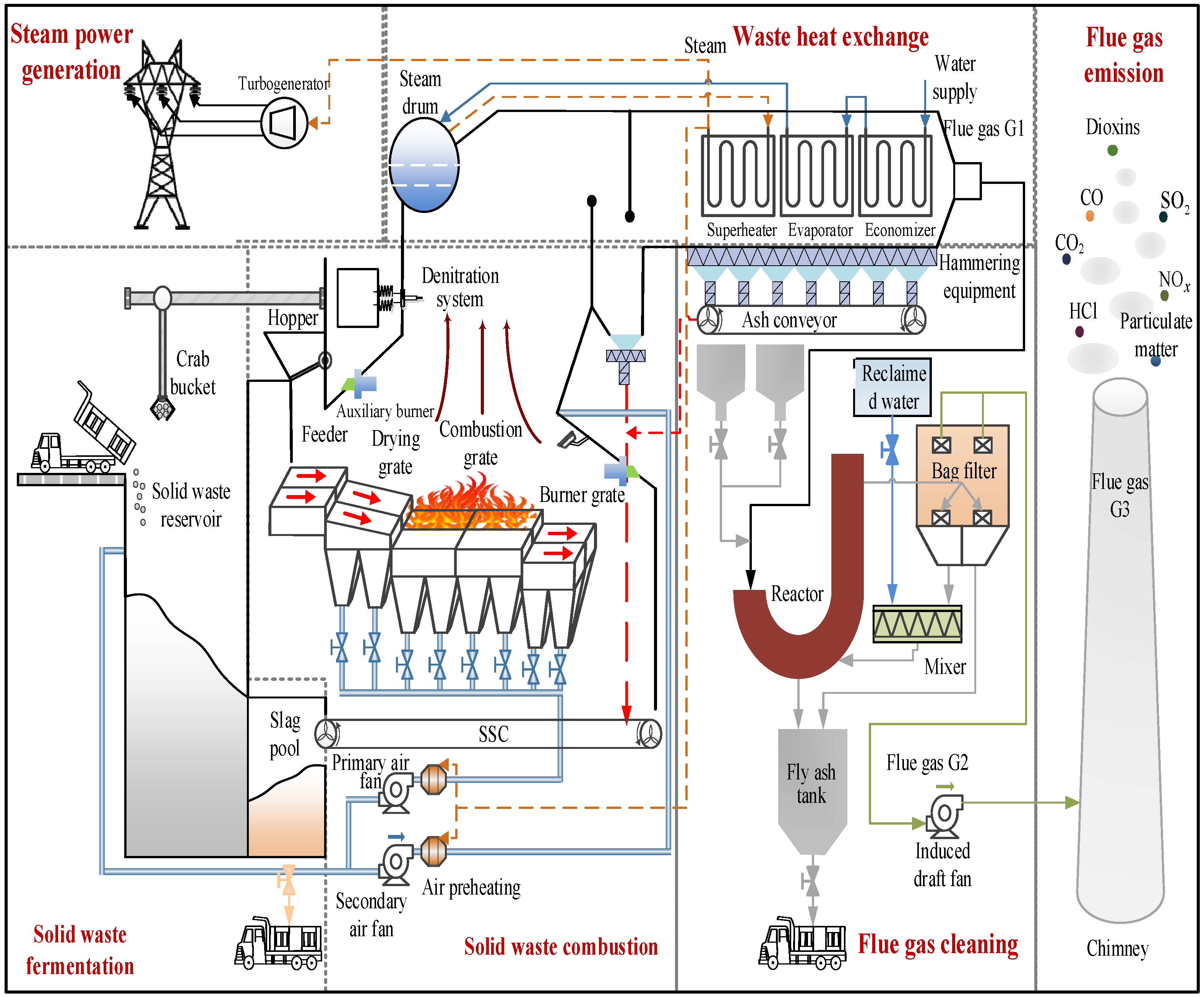
- Solid waste fermentation stage: The high moisture content in raw MSW can lead to combustion instability. Therefore, biological fermentation is required as a pretreatment to improve the calorific value. The MSW undergoes 5–7 days of aerobic fermentation in a digester, where microorganisms reduce the moisture content through metabolic processes. Organic decomposition releases biothermal energy, increasing the lower heating value by approximately 30%, which helps meet the thermal requirements of the process. After fermentation is complete, the material is transferred by a bridge-type grab crane to a sealed hopper, from which it is periodically pushed into a grate system using hydraulic feeders to initiate the combustion process.
- (2)
- Solid waste combustion stage: The energy conversion process during combustion occurs in three primary thermodynamic stages. The first stage is drying and dehydration, where secondary radiant heat from the incinerator’s arch zone interacts with primary air preheated to 120–180 °C, causing rapid evaporation of surface moisture. This phase accounts for approximately 25% to 30% of the total combustion heat consumption. Next is the main combustion stage, where the MSW enters a gas–solid two-phase combustion process once its temperature reaches the volatile matter release threshold. Between 300 °C and 850 °C, volatile matter releases combustible gases (e.g., CO and CH4) through diffusion combustion, while at higher temperatures (850 °C to 1100 °C), fixed carbon undergoes surface and pore combustion for deep oxidation. To stabilize the process, the grate movement speed is regulated, and a staged supply of air (with a 60% to 70% primary air ratio) is implemented. This ensures that the oxygen concentration remains ≥6% and the flue gas residence time is ≥2 s, effectively decomposing toxic organic compounds such as dioxins. Finally, the incineration cooling phase begins as the MSW gradually combusts and the pyrolysis rates decrease. At this stage, the remaining combustible materials are primarily composed of coke. Under high temperatures and primary air, coke undergoes oxidation with O2, releasing CO2 and water vapor. This leads to the gradual accumulation of inert substances (CO, H2O, and ash) until the MSW is completely converted into ash, marking the termination of the combustion process. The incineration ash can then be used to create a new type of environmentally friendly building material.
- (3)
- Waste heat exchange stage: After the MSW undergoes high-temperature combustion (850–1100 °C) in the incinerator, it generates flue gases with a high enthalpy (approximately 800–1000 °C) that carry 60% to 80% of the total calorific value of the MSW. The high-temperature flue gas sequentially passes through the radiant heat exchange zone (upper furnace chamber) and the convective heat exchange zone (boiler tail) of a waste heat boiler, releasing thermal energy during the recovery phase. As the core equipment for thermal energy recovery, the waste heat boiler consists of three components: an economizer, evaporator, and superheater. During operation, the economizer first utilizes residual flue gas heat to warm water from 20–80 °C to 150–200 °C, improving the system’s thermal efficiency. Next, the high-temperature flue gas transfers heat to the water in the evaporator through radiation and convection, vaporizing it into saturated steam. Finally, the steam is further heated in the superheater to reach 350–450 °C, improving its quality.
- (4)
- Steam power generation stage: The high-temperature steam produced by the waste heat boiler drives the steam turbine generator, converting mechanical energy into electrical energy. Once self-sufficiency is achieved within the plant, surplus electricity can be exported, enabling resource recycling and generating economic benefits.
- (5)
- Flue gas cleaning and emission stage: First, the denitrification system removes nitrogen oxides (NOx) from the flue gases. Next, semi-dry acid removal technology neutralizes the acidic gases in the flue gases. Subsequently, activated carbon adsorbs dioxins and heavy metals, while bag filters capture particulate matter, reactive substances, and adsorbed materials. Finally, the purified flue gases are discharged into the atmosphere through induced draft fans in compliance with national emission standards.
2.2. Methods
- (1)
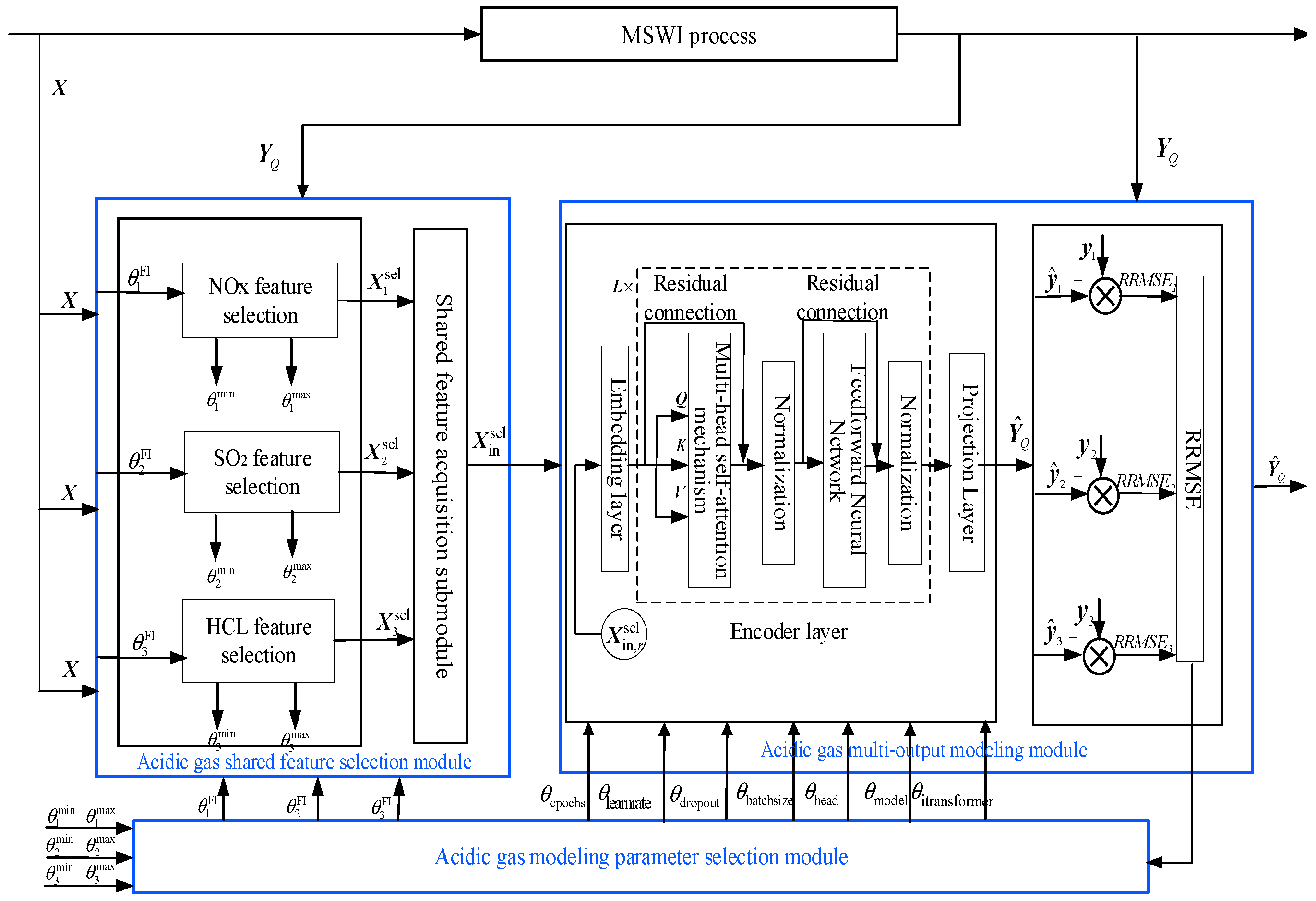
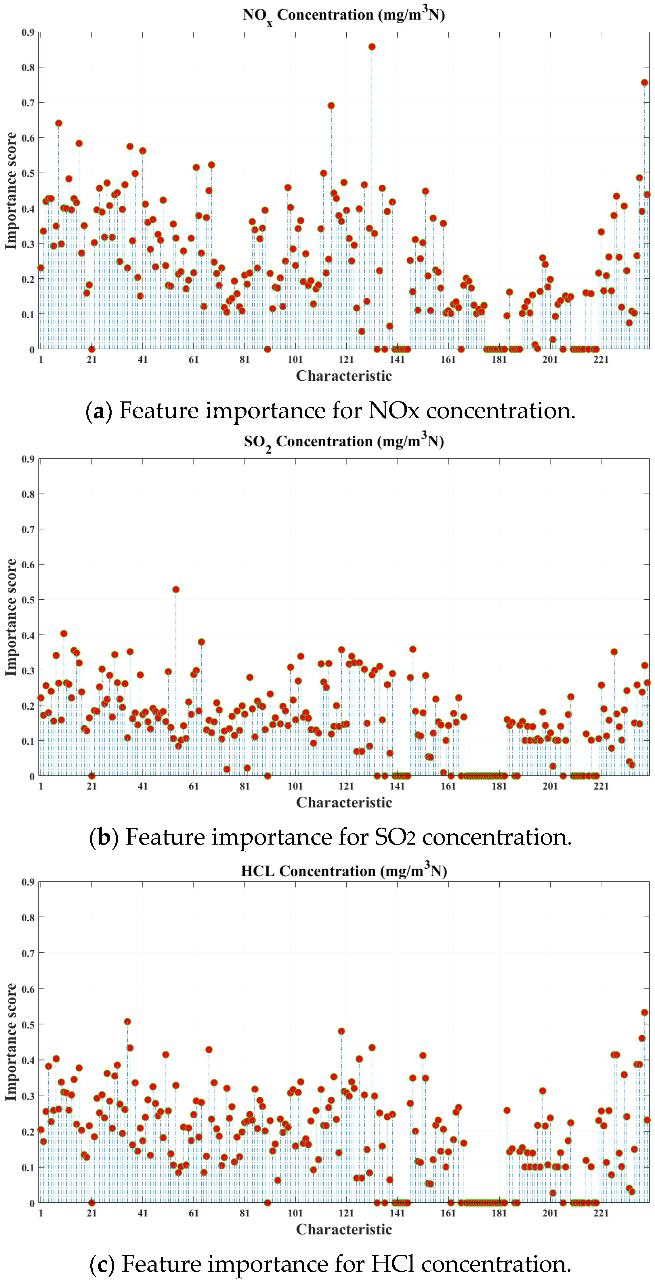
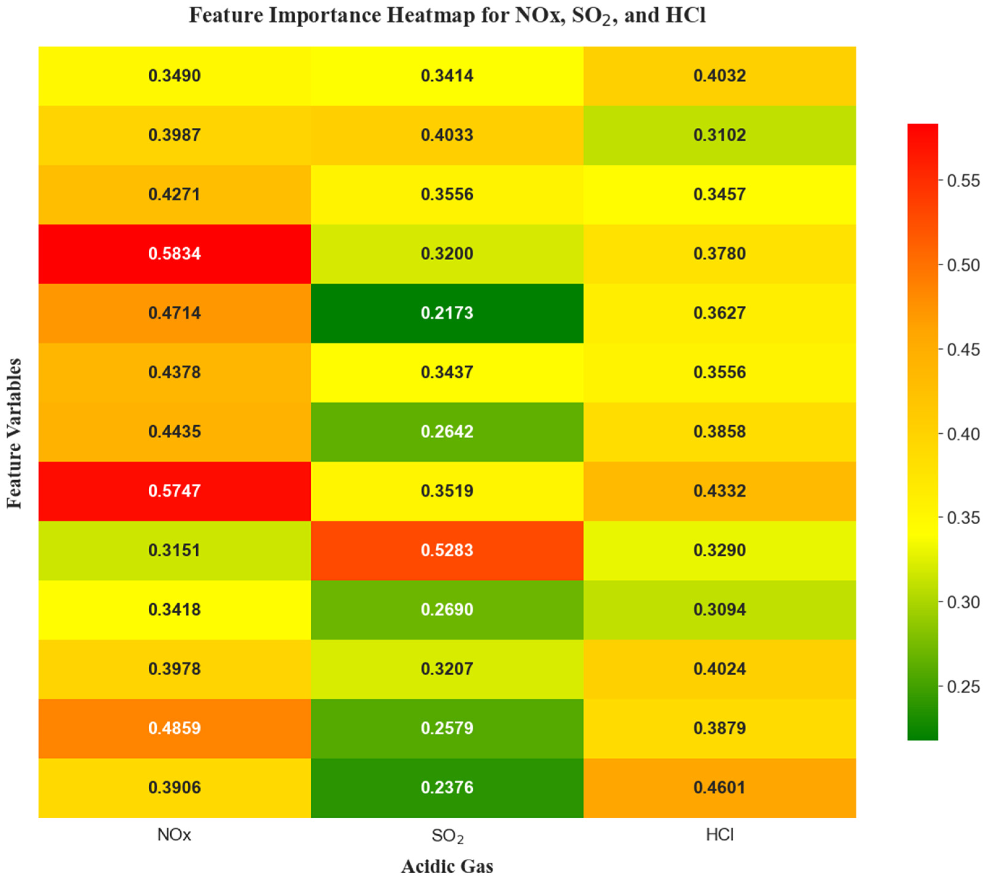
- Acidic gas shared-feature selection module: First, the contribution of each feature to the model purity is tallied at every split node across all the decision trees in the RF, which is used to calculate an overall importance score for each feature. Next, low-importance features are filtered out to reduce input dimensionality, retaining the key features to enhance model interpretability. Finally, the shared-feature acquisition submodule extracts the common features subset for the three acidic gases.
- (2)
- Acidic gas multi-output modeling module: This module uses a many-to-many ITransformer prediction model. First, the data is embedded into a 3-D tensor that is processable by the system. Then, self-attention mechanisms are utilized to capture inter-variable relationships for feature extraction. Finally, the data is passed through a feed-forward neural network, which maps the input features to a high-dimensional space via linear transformation and applies activation functions for nonlinear transformation. This process allows the model to learn more complex and richer feature representations. The RRMSE is used as the evaluation metric to quantify prediction errors and guide hyperparameter selection for the acidic gas prediction model.
- (3)
- Acidic gas modeling parameter selection module: This module selects the appropriate feature-selection parameters based on the range of feature importance values to prevent model overfitting and improve generalization.
2.2.1. Shared-Feature Selection Module for Acidic Gases
Feature Selection Sub-Module Based on RF
Redundant Feature Removal Sub-Module
2.2.2. Acidic Gas Multi-Output Modeling Module
Multi-Output ITransformer Modeling Sub-Module
- (1)
- Embedding Layer: The embedding layer maps scalar feature values into a high-dimensional semantic space, allowing the model to capture richer feature information. The computation formulas are as follows:where denotes the total number of batches; denotes the feature value dimension; and denotes the embedding operation.
- (2)
- Multi-Head Self-Attention Mechanism: The primary role of the multi-head self-attention mechanism is to enable the model to identify linear correlations and capture complex nonlinear dependencies. During the computation of each weighted output using the attention mechanism, the input data is first linearly transformed to generate the query , key , and value matrices. Taking the th encoder layer as an example, the process is as follows:where , , and are the weight matrices associated with , , and , respectively.
- (3)
- First Residual Connection: Residual connections ensure that feature information is preserved and does not degrade as it passes through multiple encoder layers, enabling the model to effectively learn deep feature interactions. The computation formula is as follows:where denotes the regularization operation.
- (4)
- First Layer Normalization: Layer normalization ensures smooth convergence during training and improves stability. The computation formulas are
- (5)
- Feed-Forward Network: The primary role of the feed-forward network is to apply nonlinear transformations and enhance features from the output of the self-attention mechanism. The computation formula is as follows:
- (6)
- Second Residual Connection: The second residual connection ensures stable information flow, facilitates gradient propagation, and works synergistically with layer normalization to support effective training of deep networks. Together with the first residual connection, it provides a dual safeguard for stable training and optimal performance in the ITransformer architecture. The computation formula is as follows:
- (7)
- Second Layer Normalization: The computation formulas are
- (8)
- Projection Layer: A fully connected layer maps the flattened 2-D feature matrix to the final prediction target space, computing output values for the th batch as follows:where is the weight matrix for the multiple outputs and is the bias matrix for the multiple outputs.
Multi-Output Evaluation Metric Acquisition Submodule
2.2.3. Acidic Gas Modeling Parameter Selection Module
2.3. Pseudocode
| Algorithm 1: RF-ITransformer | |
| Step1: | Input: dataset , ITransformer model iterations , ITransformer model learning rate , ITransformer model dropout rate ; |
| Step2: | Calculate the feature importance threshold based on the following Equations (1)–(4); |
| Step3: | According to Equation (5), the feature set satisfying the conditions is selected based on the set characteristic threshold ; |
| Step 4: | Calculate the shared features according to Equations (6)–(18), yielding ; |
| Step 5: | For to Use the sequence data from the -th batch as the model input; |
| Step 6: | Based on Equations (19)–(27), the result after the embedding layer is calculated as ; |
| Step 7: | Pass the of the -th batch through the self-attention mechanism of the -th encoder layer, and compute the -th head self-attention result according to Equations (28)–(32); |
| Step 8: | Based on Equations (33) and (34), the result of the multi-head self-attention mechanism is calculated as ; |
| Step 9: | According to Equation (35), the result of the first-layer residual connection is calculated as ; |
| Step 10: | Use Equations (36)–(39), compute the first-layer normalization result in the -th encoder layer for the -th batch; |
| Step 11: | Use Equations (40) and (41), compute the feed-forward neural network output in the -th embedding layer for the -th batch; |
| Step 12: | Use Equation (42), compute the second-layer residual connection result ; |
| Step 13: | Use Equations (43)–(46), compute the second-layer normalization result in the -th encoder layer for the -th batch; |
| Step 14: | Use Equations (47)–(49), compute the predicted outputs for the -th batch samples; |
| Step 15: | Use Equations (50) and (51), compute the final ITransformer model output as ; |
| Step 16: | Use Equations (52) and (53), quantify the multi-output ITransformer model with the computed ; |
| Step 17: | Adjust the appropriate hyperparameter combination according to Equations (54) and (55); |
| Step 18: | end; |
| Step 19: | The above steps yield the model; |
3. Results
3.1. Performance Metrics
3.2. Experimental Results
3.2.1. Feature Selection
3.2.2. Prediction Model
3.3. Method Comparison
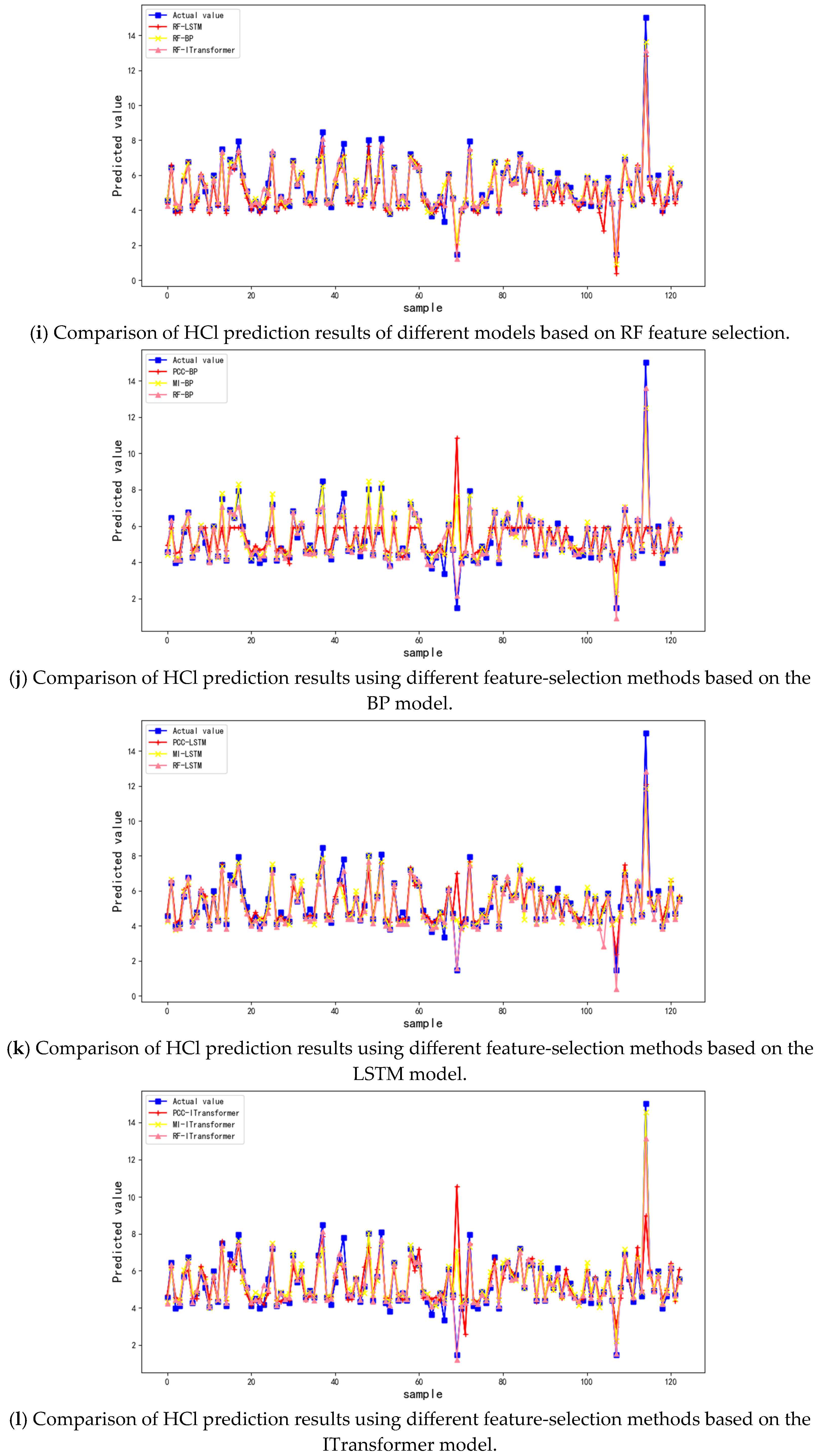
3.3.1. Experimental Comparison of Feature Selection
3.3.2. Experimental Comparison of Prediction Models
3.4. Hyperparameter Analysis
- (1)
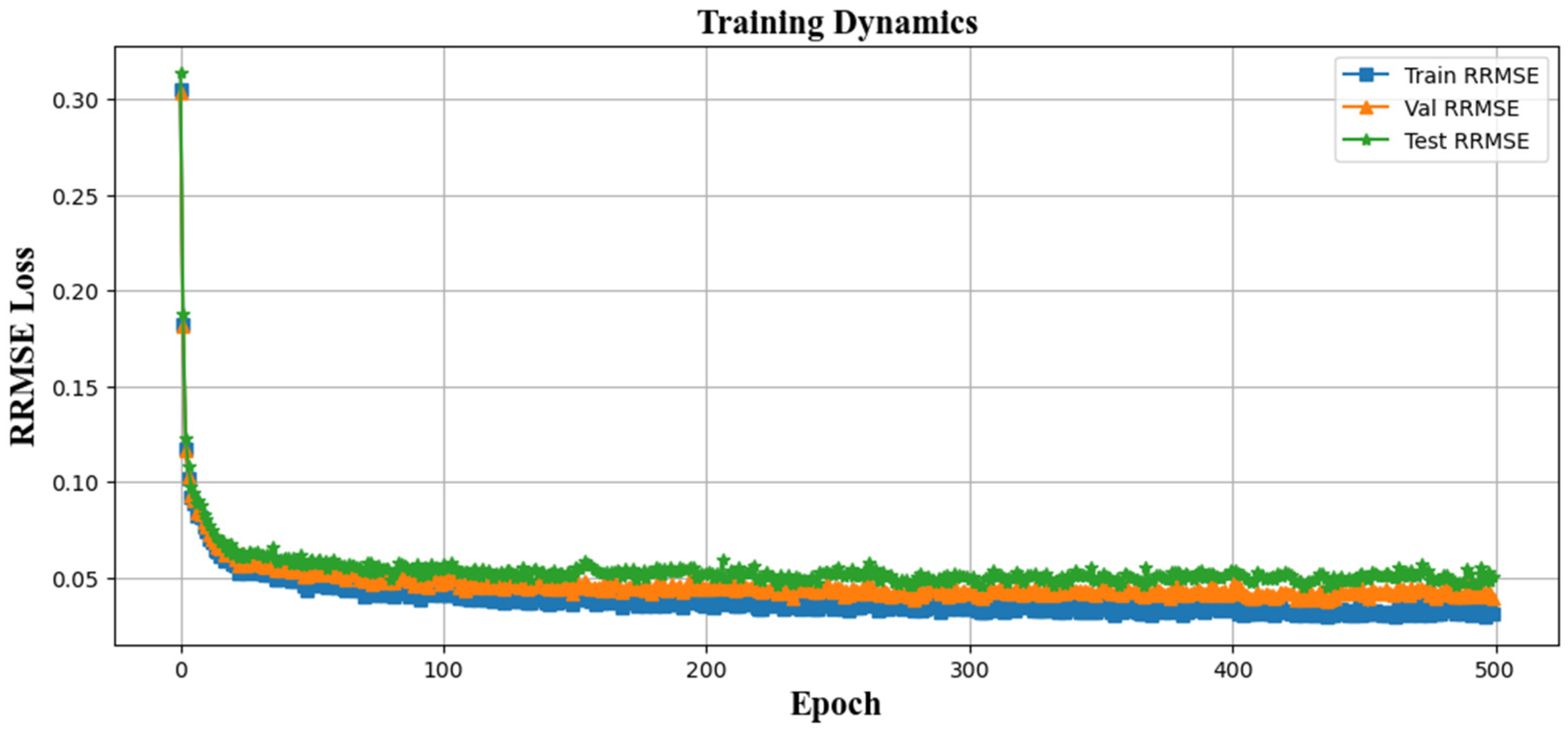
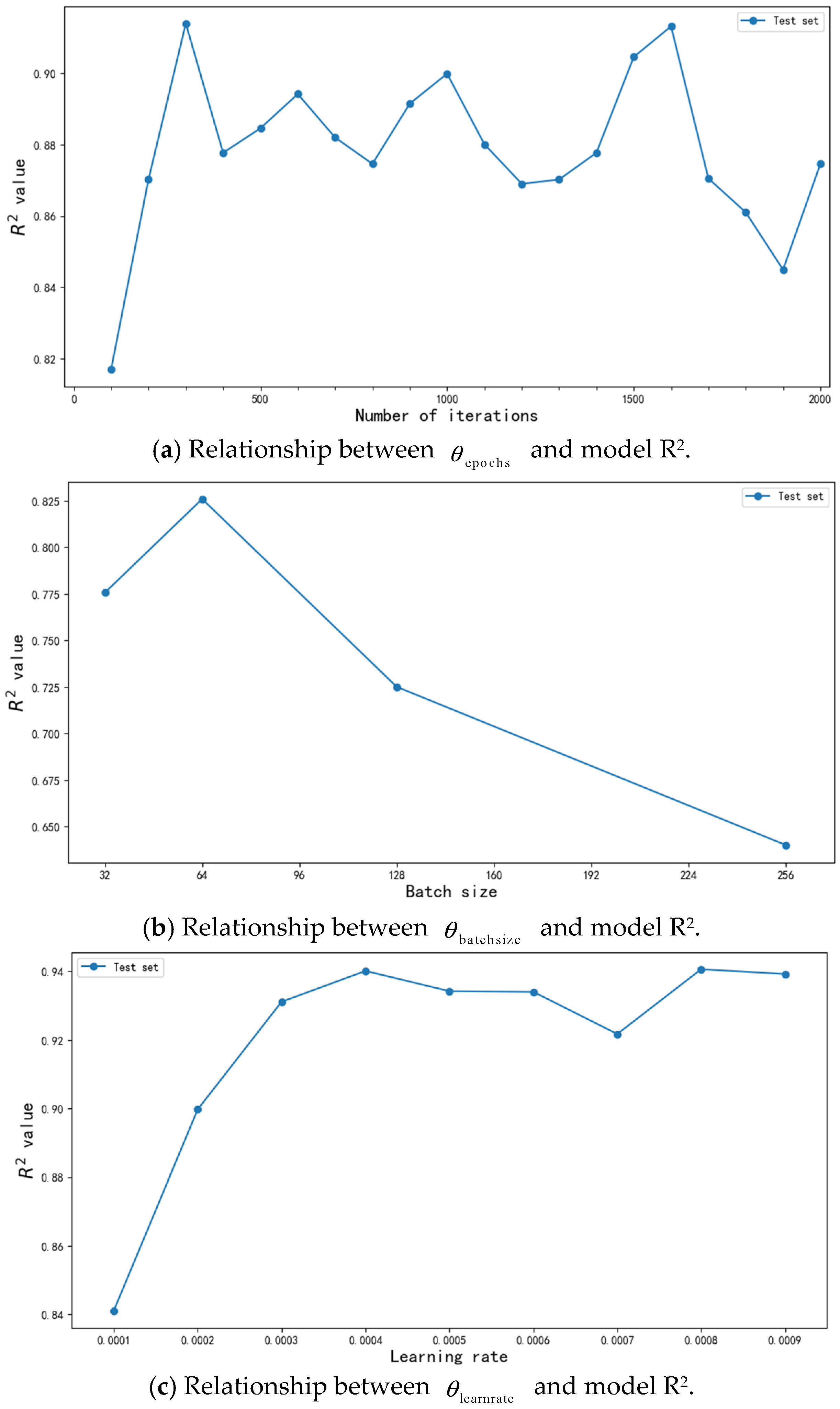
- Number of iterations: Increasing the number of iterations lengthens the model’s runtime. However, the prediction accuracy did not improve significantly with additional training. Therefore, an optimal value should be chosen to minimize training time while maintaining high accuracy. A value of 300 iterations was found to be optimal.
- (2)
- Batch size: The batch size is a crucial hyperparameter that determines how many samples are used in each model update. Selecting an appropriate batch size is essential for training efficiency. A batch size of 64 yielded the best weight-update performance and highest prediction accuracy.
- (3)
- Learning rate: A suitable learning rate enables the objective function to converge to a local minimum within a reasonable time. Most networks initialize the learning rate at 0.01 or 0.001. In this study, learning rates from 0.001 to 0.01, in steps of 0.001, were tested. The highest accuracy was achieved at a learning rate of 0.004.
- (4)
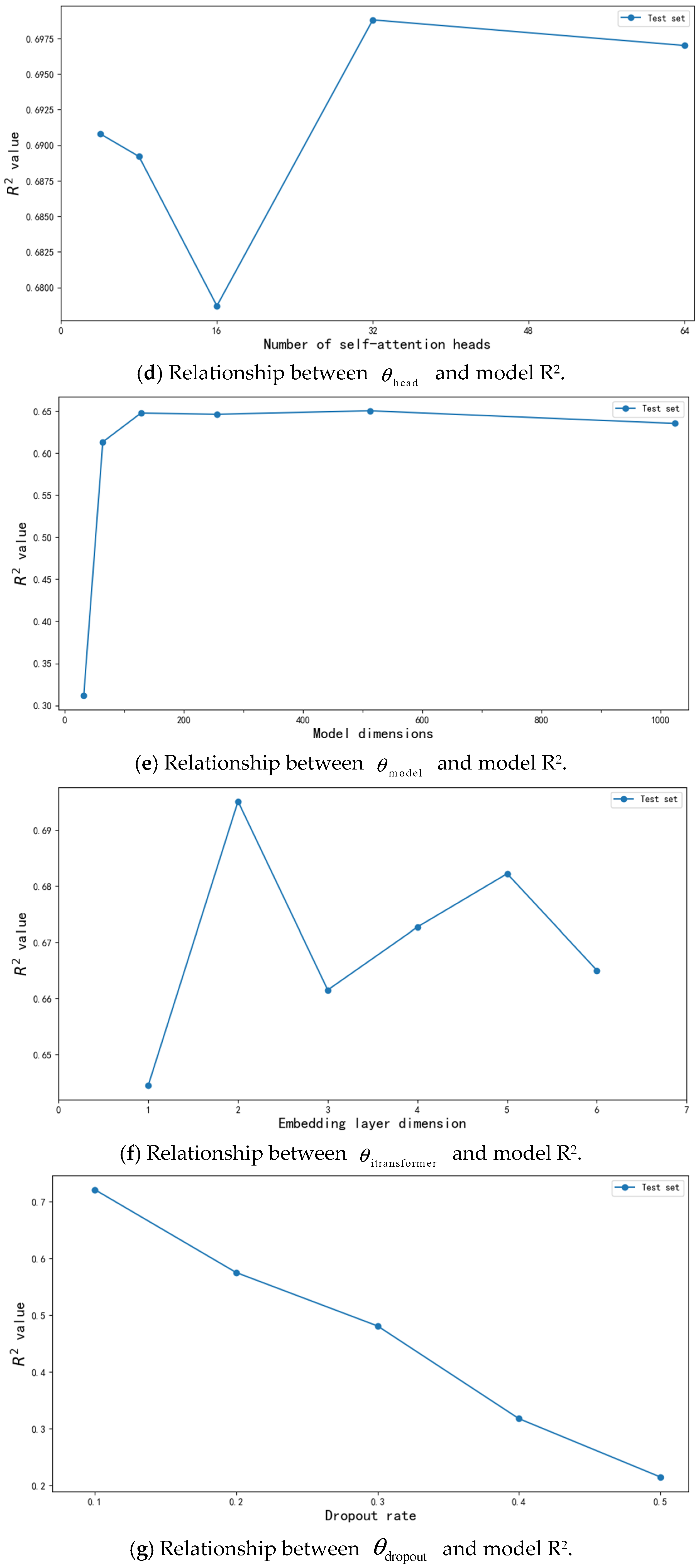
- Model dimensions: The number of dimensions governs the model’s representational capacity, complexity, and computational efficiency. Increasing the number of dimensions only provided marginal performance gains while extending the runtime. Therefore, the dimension was set to 128.
- (5)
- Encoder layers: In ITransformer, the number of encoder layers directly impacts the model’s complexity and performance. By adjusting the layer count, the model can capture more complex patterns and fit intricate data distributions. Starting with a baseline of 1, the experiments added layers incrementally up to 5. The best predictive performance was achieved with 2 layers, so the model was accordingly set to 2.
- (6)
- Self-attention heads: This parameter determines the model’s ability to attend to different types of information simultaneously. In ITransformer, the head count directly influences the model’s capacity to capture complex relationships among multivariate features. The optimal performance was observed at 32 heads, so the value was set to 32.
- (7)
- Dropout rate: Dropout randomly deactivates neurons with a given probability, which enhances generalization. As dropout increased, there was a general decline in accuracy. Therefore, the dropout rate was set to 0.1.
- (8)
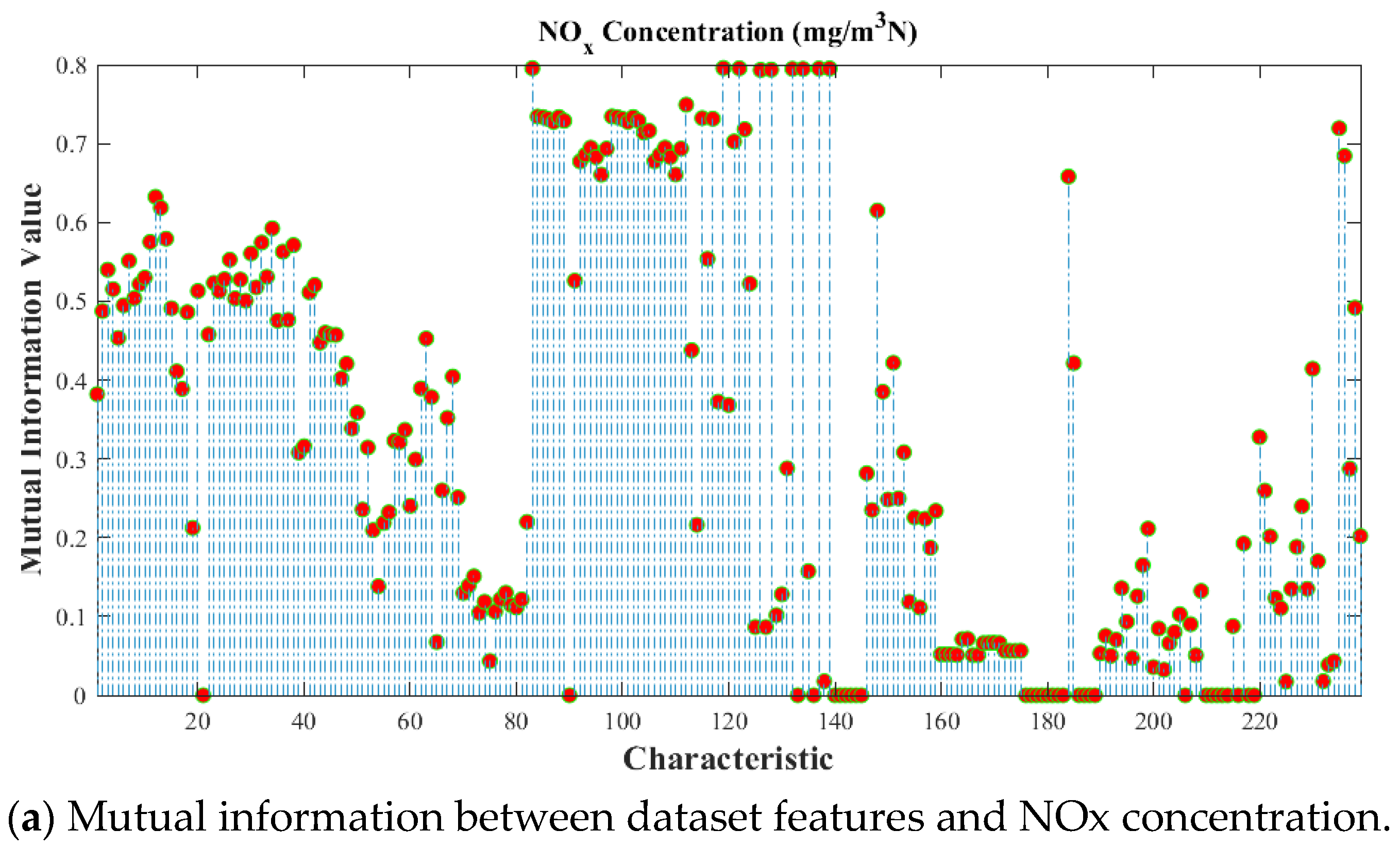
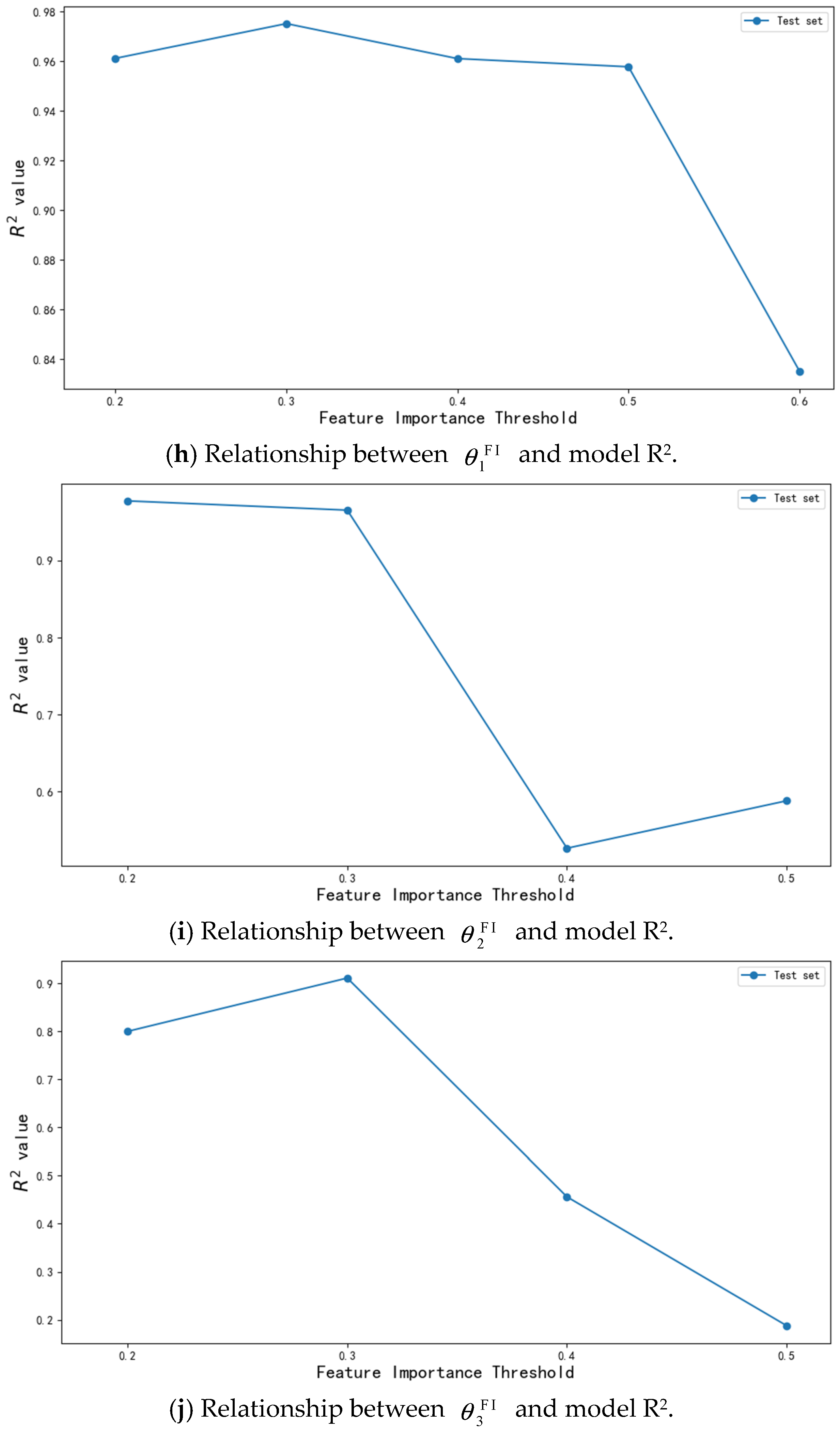
- RF threshold (NOx): This key parameter for feature selection in Random Forests identifies strongly correlated variables, optimizing the prediction accuracy. The accuracy first increased and then decreased with rising thresholds, so the value was set to 0.3.
- (9)
- RF threshold (SO2): The accuracy peaked when the threshold was set to 0.2.
- (10)
- RF threshold (HCl): The accuracy declined as the threshold increased, so the value was set to 0.3.
4. Conclusions
Author Contributions
Funding
Institutional Review Board Statement
Informed Consent Statement
Data Availability Statement
Conflicts of Interest
Abbreviations
| MSW | Municipal solid waste |
| MSWI | Municipal solid waste incineration |
| RF | Random Forest |
| ITransformer | Inverted Transformer |
| COPD | Chronic obstructive pulmonary disease |
| CEMS | Continuous emission monitoring system |
| LSTM | Long Short-Term Memory |
| MI | Mutual information |
| PSO | Particle swarm optimization algorithm |
| FAR | Fast attribute reduction |
| HK-ELM | Hybrid kernel extreme learning machine |
| AMNN | Attention modular neural network |
| ARMAX | Autoregressive sliding average model |
| SNCR | Selective Non-Catalytic Reduction |
| RRMSE | Relative root-mean-square error |
| RMAE | Root mean absolute error |
| FI | Feature importance |
| OOB | Out-of-bag |
| BP | Back propagation |
| MIC | Maximal information coefficient |
| PCA | Principal component analysis |
Appendix A

| Num | Symbol | Actual Meaning |
|---|---|---|
| 1. | Original sample input dataset | |
| 2. | Dataset after random forest feature selection targeting NOx | |
| 3. | Dataset after random forest feature selection targeting SO2 | |
| 4. | Dataset after random forest feature selection targeting HCl | |
| 5. | Random forest feature-selection threshold with NOx as the target variable | |
| 6. | Random forest feature-selection threshold with SO2 as the target variable | |
| 7. | Random forest feature-selection threshold with HCl as the target variable | |
| 8. | The predictions of NOx based on after random forest feature selection | |
| 9. | The predictions of SO2 based on after random forest feature selection | |
| 10. | The predictions of HCl based on after random forest feature selection | |
| 11. | Matrix containing output | |
| 12. | Actual output | |
| 13. | Number of training epochs in ITransformer | |
| 14. | Learning rate of ITransformer | |
| 15. | Dropout rate of ITransformer | |
| 16. | Model dimension of ITransformer | |
| 17. | Number of embedding layers in ITransformer | |
| 18. | Number of self-attention heads of ITransformer | |
| 19. | Sample count of the original input dataset | |
| 20. | Feature count of the original sample input dataset | |
| 21. | Number of features for NOx as the target variable after RF feature selection | |
| 22. | Number of features for SO2 as the target variable after RF feature selection | |
| 23. | Number of features for HCl as the target variable after RF feature selection | |
| 24. | Shared feature set after redundancy removal | |
| 25. | Number of features in the common feature set after redundancy removal | |
| 26. | Empirically determined maximum RF feature selection threshold for NOx | |
| 27. | Empirically determined minimum RF feature selection threshold for NOx | |
| 28. | Empirically determined maximum RF feature selection threshold for SO2 | |
| 29. | Empirically determined minimum RF feature selection threshold for SO2 | |
| 30. | Empirically determined maximum RF feature selection threshold for HCl | |
| 31. | Empirically determined minimum RF feature selection threshold for HCl | |
| 32. | Empirically determined minimum iteration count | |
| 33. | Empirically determined maximum iteration count | |
| 34. | Empirically determined minimum dropout rate | |
| 35. | Empirically determined maximum dropout rate | |
| 36. | Empirically determined minimum learning rate | |
| 37. | Empirically determined maximum learning rate | |
| 38. | Empirically determined minimum batch size | |
| 39. | Empirically determined maximum batch size | |
| 40. | Empirically determined minimum model dimension | |
| 41. | Empirically determined maximum model dimension | |
| 42. | Empirically determined minimum number of encoder layers | |
| 43. | Empirically determined maximum number of encoder layers | |
| 44. | Empirically determined maximum number of self-attention heads | |
| 45. | Empirically determined maximum number of self-attention heads | |
| 46. | Relative root-mean-square error | |
| 47. | Decision tree model | |
| 48. | Number of decision trees | |
| 49. | Feature with index for the th acidic gas | |
| 50. | Node split threshold for the th acidic gas | |
| 51. | Optimal split feature index for the th acidic gas | |
| 52. | Optimal split threshold for the th acidic gas | |
| 53. | Number of left children of the feature split node for the th acidic gas | |
| 54. | Number of right children of the feature split node for the th acidic gas | |
| 55. | Out-of-bag prediction error for the th acidic gas | |
| 56. | Prediction error on perturbed out-of-bag data with index for the th acidic gas | |
| 57. | The importance value of the feature with index in the th acidic gas | |
| 58. | Set of feature variable names for target variable NOx | |
| 59. | Set of feature variable names for target variable SO2 | |
| 60. | Set of feature variable names for target variable HCl | |
| 61. | Comparison criterion for and | |
| 62. | Comparison criterion for and | |
| 63. | Comparison criterion for and | |
| 64. | Comparison criterion for and | |
| 65. | Comparison criterion for and | |
| 66. | The th batch of samples inputted into the ITransformer model | |
| 67. | Total number of batches | |
| 68. | Feature dimensions | |
| 69. | Positional encoding for odd indices | |
| 70. | Positional encoding for even indices | |
| 71. | High-dimensional data after the embedding layer | |
| 72. | Enhanced representation containing positional information | |
| 73. | Query vector | |
| 74. | Key vector | |
| 75. | Value vector | |
| 76. | Weight of the query vector | |
| 77. | Weight of the key vector | |
| 78. | Weight of the value vector | |
| 79. | Key matrix dimension | |
| 80. | The output of the th self-attention head in the th encoder layer under batch | |
| 81. | The multi-head self-attention in the th encoder layer under batch | |
| 82. | Output projection matrix | |
| 83. | Output of the first residual connection | |
| 84. | Denotes the mean of | |
| 85. | Denotes the variance of the first normalization layer | |
| 86. | Scaling parameter of the first normalization layer | |
| 87. | Shift parameter of the first normalization layer | |
| 88. | Used for division-by-zero prevention in the first normalization layer | |
| 89. | Output of the first normalization layer in encoder layer for batch | |
| 90. | Output of the feed-forward network in encoder layer for batch | |
| 91. | Output of the second residual connection | |
| 92. | Mean of | |
| 93. | Variance of the second normalization layer | |
| 94. | Scaling parameter of the second normalization layer | |
| 95. | Shift parameter of the second normalization layer | |
| 96. | Used for division-by-zero prevention in the second normalization layer | |
| 97. | Output of the th encoder layer for batch | |
| 98. | Output after flattening | |
| 99. | The th output value for batch | |
| 100. | Predicted result | |
| 101. | Actual value of the th sample | |
| 102. | Predicted output of the th sample | |
| 103. | Average of actual values | |
| 104. | ITransformer-based model | |
| 105. | RF-ITransformer-based model |
| Num | Variable Name | Unit | Feature Importance |
|---|---|---|---|
| 1. | Primary combustion chamber right flue gas temperature | 1 °C | 0.4192 |
| 2. | Primary combustion chamber left flue gas temperature 2 | °C | 0.4272 |
| 3. | Primary combustion chamber middle flue gas temperature 2 | °C | 0.4270 |
| 4. | Primary combustion chamber middle flue gas temperature 1 | °C | 0.3347 |
| 5. | Primary combustion chamber left flue gas temperature 3 | °C | 0.3490 |
| 6. | Primary combustion chamber middle flue gas temperature 3 | °C | 0.6407 |
| 7. | Top gas temperature at burnout grate 1 | °C | 0.3987 |
| 8. | Temperature of left primary combustion chamber | °C | 0.3950 |
| 9. | Average temperature of primary combustion chamber | °C | 0.4271 |
| 10. | Left inner temperature of drying grate | °C | 0.4155 |
| 11. | Left outer temperature of drying grate | °C | 0.5834 |
| 12. | Right outer temperature of drying grate | °C | 0.3502 |
| 13. | Left inner temperature of combustion grate 1-1 | °C | 0.3950 |
| 14. | Right inner temperature of combustion grate 1-1 | °C | 0.3887 |
| 15. | Right outer temperature of combustion grate 1-1 | °C | 0.3177 |
| 16. | Left outer temperature of combustion grate 1-1 | °C | 0.4562 |
| 17. | Left inner temperature of combustion grate 1-2 | °C | 0.4714 |
| 18. | Left outer temperature of combustion grate 1-2 | °C | 0.4070 |
| 19. | Right outer temperature of combustion grate 1-2 | °C | 0.4378 |
| 20. | Left inner temperature of combustion grate 2-1 | °C | 0.4435 |
| 21. | Right outer temperature of combustion grate 2-1 | °C | 0.4663 |
| 22. | Right inner temperature of combustion grate 2-1 | °C | 0.3966 |
| 23. | Right outer temperature of combustion grate 2-2 | °C | 0.4980 |
| 24. | Left outer temperature of combustion grate 2-2 | °C | 0.5747 |
| 25. | Right inner temperature of combustion grate 2-2 | °C | 0.3073 |
| 26. | Left flue gas temperature of first pass | °C | 0.5623 |
| 27. | Right flue gas temperature of first pass | °C | 0.4112 |
| 28. | Left inlet flue gas temperature of protection tube | °C | 0.3597 |
| 29. | Left inlet flue gas temperature of tertiary superheater | °C | 0.3676 |
| 30. | Left inlet flue gas temperature of evaporator | °C | 0.3255 |
| 31. | Right inlet flue gas temperature of evaporator | °C | 0.3091 |
| 32. | Left inlet flue gas temperature of economizer | °C | 0.4226 |
| 33. | Combustion grate inlet air temperature (burn 1-1, 2 + 2-1) | °C | 0.3547 |
| 34. | Drying grate inlet air temperature | °C | 0.3151 |
| 35. | Inlet biogas pressure | KPa | 0.3146 |
| 36. | Drying section outlet air temperature | °C | 0.5152 |
| 37. | Combustion zone outlet air temperature | °C | 0.3785 |
| 38. | Primary superheater outlet steam temperature | °C | 0.3731 |
| 39. | Secondary superheater outlet steam temperature | °C | 0.4495 |
| 40. | Tertiary superheater outlet steam temperature | °C | 0.5226 |
| 41. | Left drying grate 1 (air flow setpoint) | km3N/h | 0.3615 |
| 42. | Left drying grate 2 (air flow setpoint) | km3N/h | 0.3385 |
| 43. | Left combustion grate 1-2 (air flow setpoint) | km3N/h | 0.3132 |
| 44. | Left combustion grate 2-1 (air flow setpoint) | km3N/h | 0.3430 |
| 45. | Left combustion grate 2-2 (air flow setpoint) | km3N/h | 0.3938 |
| 46. | Left drying grate 1 air flow | km3N/h | 0.4580 |
| 47. | Right drying grate 1 air flow | km3N/h | 0.4018 |
| 48. | Combustion zone grate right section 1-1 air flow | km3N/h | 0.3646 |
| 49. | Combustion zone grate left section 1-1 air flow | km3N/h | 0.3418 |
| 50. | Burnout zone right grate air flow | km3N/h | 0.3413 |
| 51. | Boiler #2 secondary air total accumulation | km3N | 0.4988 |
| 52. | Economizer total feedwater flow | t/h | 0.6906 |
| 53. | Economizer No. 2 feedwater flow | t/h | 0.4425 |
| 54. | Economizer No. 1 feedwater flow | t/h | 0.4274 |
| 55. | Primary superheater cooling water flow | t/h | 0.3788 |
| 56. | Primary superheater cooling water flow accumulation | t | 0.3625 |
| 57. | Secondary superheater cooling water flow | t/h | 0.4728 |
| 58. | Total primary and secondary superheater attemperation water | t/h | 0.3935 |
| 59. | Boiler main steam total accumulation | t | 0.3141 |
| 60. | Mixer feedwater flow A accumulation | kg | 0.3978 |
| 61. | Mixer feedwater flow B accumulation | kg | 0.4661 |
| 62. | FGD reactor inlet flue gas flow B | km3N/h | 0.3427 |
| 63. | Urea solution supply flow | L/h | 0.8573 |
| 64. | Urea solution supply flow accumulation | L | 0.3281 |
| 65. | Total feed into lime feeder | kg | 0.3904 |
| 66. | Total feed into activated carbon silo | kg | 0.4174 |
| 67. | Amount of urea dilution solution injected into the furnace | L/h | 0.4562 |
| 68. | Top temperature of grate in burnout zone 2 | °C | 0.4004 |
| 69. | Cumulative feed amount from activated carbon storage silo | kg | 0.4174 |
| 70. | Furnace negative pressure | Pa | 0.3109 |
| 71. | Boiler drum pressure | MPa | 0.3017 |
| 72. | Steam pressure at outlet of tertiary superheater | MPa | 0.4479 |
| 73. | Reactor outlet differential pressure A | Pa | 0.3714 |
| 74. | Bag filter differential pressure B | Pa | 0.3566 |
| 75. | Secondary air fan current | A | 0.3326 |
| 76. | Grate hydraulic pump 2 current | A | 0.3790 |
| 77. | Grate hydraulic pump 3 current | A | 0.4338 |
| 78. | Primary air fan frequency | Hz | 0.4058 |
| 79. | Flue gas oxygen concentration | % | 0.4859 |
| 80. | Flue gas oxygen concentration | % | 0.3906 |
| 81. | Flue gas oxygen concentration | % | 0.7559 |
| 82. | Flue gas dust concentration | mg/m3N | 0.4383 |
| Num | Variable Name | Unit | Feature Importance |
|---|---|---|---|
| 1. | Primary combustion chamber left flue gas temperature 1 | °C | 0.2211 |
| 2. | Primary combustion chamber right flue gas temperature 1 | °C | 0.2559 |
| 3. | Primary combustion chamber middle flue gas temperature 2 | °C | 0.2398 |
| 4. | Primary combustion chamber left flue gas temperature 3 | °C | 0.3414 |
| 5. | Burnout grate top air temperature | °C | 0.4033 |
| 6. | Burnout grate top air temperature | °C | 0.2637 |
| 7. | Primary combustion chamber average temperature | °C | 0.3556 |
| 8. | Drying grate left inner temperature | °C | 0.3486 |
| 9. | Drying grate left outer temperature | °C | 0.3200 |
| 10. | Drying grate right inner temperature | °C | 0.2381 |
| 11. | Combustion grate 1-1 left outer temperature | °C | 0.2521 |
| 12. | Combustion grate 1-1 right outer temperature | °C | 0.2045 |
| 13. | Combustion grate 1-2 left inner temperature | °C | 0.2173 |
| 14. | Combustion grate 1-2 left outer temperature | °C | 0.2849 |
| 15. | Combustion grate 1-2 right outer temperature | °C | 0.3437 |
| 16. | Combustion grate 2-1 left inner temperature | °C | 0.2642 |
| 17. | Combustion grate 2-1 left outer temperature | °C | 0.2178 |
| 18. | Combustion grate 2-2 left outer temperature | °C | 0.3519 |
| 19. | Right slag outlet temperature | °C | 0.2861 |
| 20. | Economizer outlet flue gas temperature | °C | 0.2955 |
| 21. | Drying grate inlet air temperature | °C | 0.5283 |
| 22. | Grate right cooling air outlet temperature | °C | 0.2096 |
| 23. | Outlet biogas pressure | KPa | 0.2874 |
| 24. | Drying section outlet air temperature | °C | 0.2990 |
| 25. | Drying section biogas flow | m3/h | 0.3797 |
| 26. | Inlet flue gas temperature 1 | °C | 0.2072 |
| 27. | Unit 2 primary air total flow | km3N | 0.2791 |
| 28. | Left combustion grate 1-1 (air flow setpoint) | km3N/h | 0.2122 |
| 29. | Right drying grate 1 (air flow setpoint) | km3N/h | 0.2321 |
| 30. | Right drying grate 1 air flow | km3N/h | 0.3079 |
| 31. | Left drying grate 2 air flow | km3N/h | 0.2148 |
| 32. | Combustion grate left section 1-1 air flow | km3N/h | 0.2690 |
| 33. | Unit 2 secondary air total flow | km3N | 0.2661 |
| 34. | Secondary air flow | km3N/h | 0.2507 |
| 35. | Secondary air fan branch 1 flow | km3N/h | 0.3186 |
| 36. | Boiler main steam totalized flow | t | 0.3169 |
| 37. | Boiler outlet main steam flow | t/h | 0.3389 |
| 38. | Mixer feed water flow A accumulation | kg | 0.3207 |
| 39. | Mixer feed water flow B accumulation | kg | 0.3022 |
| 40. | Urea solvent supply flow accumulation | L | 0.2990 |
| 41. | Furnace #2 urea solution accumulation | L | 0.3106 |
| 42. | Lime feeder accumulation | kg | 0.2586 |
| 43. | Activated carbon silo feed accumulation | kg | 0.2899 |
| 44. | Primary air fan outlet air pressure | KPa | 0.2786 |
| 45. | Secondary air fan outlet air pressure | KPa | 0.3590 |
| 46. | Level 3 superheater outlet steam pressure | MPa | 0.2844 |
| 47. | Reactor differential pressure B | Pa | 0.2176 |
| 48. | Drying grate left outer speed | % | 0.2214 |
| 49. | Secondary air fan inlet damper opening (actual value) | % | 0.2242 |
| 50. | Secondary air fan current | A | 0.2573 |
| 51. | Grate hydraulic pump 2 current | A | 0.3516 |
| 52. | Secondary air fan frequency | HZ | 0.2416 |
| 53. | Flue gas oxygen concentration | % | 0.2579 |
| 54. | Flue gas oxygen concentration | % | 0.2376 |
| 55. | Flue gas oxygen concentration | % | 0.3130 |
| 56. | Flue gas dust concentration | mg/m3N | 0.2639 |
| 57. | Reactor differential pressure B | Pa | 0.2176 |
| Num | Variable Name | Unit | Feature Importance |
|---|---|---|---|
| 1. | Flue gas temperature 2, left side of primary combustion chamber | °C | 0.3826 |
| 2. | Flue gas temperature 3, left side of primary combustion chamber | °C | 0.4032 |
| 3. | Flue gas temperature 3, right side of primary combustion chamber | °C | 0.3381 |
| 4. | Top air temperature at the grate end of the burnout zone | °C | 0.3102 |
| 5. | Left side temperature of primary combustion chamber | °C | 0.3023 |
| 6. | Average temperature of primary combustion chamber | °C | 0.3457 |
| 7. | Drying grate left outer temperature | °C | 0.3780 |
| 8. | Combustion grate 1-2 left inner temperature | °C | 0.3627 |
| 9. | Combustion grate 1-2 right outer temperature | °C | 0.3556 |
| 10. | Combustion grate 2-1 left inner temperature | °C | 0.3858 |
| 11. | Combustion grate 2-2 left inner temperature | °C | 0.5071 |
| 12. | Combustion grate 2-2 left outer temperature | °C | 0.4332 |
| 13. | Combustion grate 2-2 right outer temperature | °C | 0.3364 |
| 14. | Level 3 superheater left inlet flue gas temperature | °C | 0.3254 |
| 15. | Economizer right inlet flue gas temperature | °C | 0.4144 |
| 16. | Drying grate inlet air temperature | °C | 0.3290 |
| 17. | Level 2 superheater outlet steam temperature | °C | 0.4284 |
| 18. | Economizer outlet water temperature | °C | 0.3366 |
| 19. | FGD bag filter B inlet temperature | °C | 0.3209 |
| 20. | Left drying grate 2 (air setpoint) | km3N/h | 0.3184 |
| 21. | Left drying grate 2 air flow | km3N/h | 0.3173 |
| 22. | Combustion grate left section 1-1 air flow | km3N/h | 0.3094 |
| 23. | Economizer No. 2 feedwater flow | t/h | 0.3531 |
| 24. | Level 2 superheater cooling water flow | t/h | 0.3123 |
| 25. | Total Level 1 and 2 superheater attemperation water | t/h | 0.3082 |
| 26. | Boiler outlet main steam flow | t/h | 0.4800 |
| 27. | Mixer feedwater flow A cumulative | kg | 0.4024 |
| 28. | Urea solution supply flow | L/h | 0.4342 |
| 29. | Secondary air fan outlet air pressure | KPa | 0.3497 |
| 30. | Boiler drum pressure | MPa | 0.4119 |
| 31. | Level 3 superheater outlet steam pressure | MPa | 0.3492 |
| 32. | Left burnout grate air duct damper opening (actual) | % | 0.3137 |
| 33. | Grate hydraulic pump 3 current | A | 0.4138 |
| 34. | Primary air fan frequency | Hz | 0.3590 |
| 35. | Flue gas oxygen concentration | % | 0.3879 |
| 36. | Flue gas oxygen concentration | % | 0.4601 |
| 37. | Flue gas temperature 2, left side of primary combustion chamber | % | 0.5326 |
References
- Yin, D.; Zhao, J.; Liu, J.-W.; Zhou, J.; Cheng, L.; Zhao, J. A review of China’s municipal solid waste (MSW) and comparison with international regions: Management and technologies in treatment and resource utilization. J. Clean. Prod. 2021, 293, 126144. [Google Scholar] [CrossRef] [Scilit]
- Clemente, E.; Domingues, E.; Quinta-Ferreira, R.M.; Leitão, A.; Martins, R.C. European and African landfilling practices: An overview on MSW management, leachate characterization, and treatment technologies. J. Water Process Eng. 2024, 66, 105931. [Google Scholar] [CrossRef] [Scilit]
- Aghabeyk, F.; Chen, B.; Brito van Zijl, M.; Ye, G. Physicochemical characterization and resource recovery potential of hazardous municipal solid waste incineration (MSWI) fly ash and air pollution control (APC) residues in the Netherlands. J. Environ. Manag. 2025, 384, 125579. [Google Scholar] [CrossRef] [Scilit] [PubMed]
- Chen, A.; Chen, J.; Cui, J.; Fan, C.; Han, W. Research on the Risk and Countermeasures of “Garbage Surrounding Cities” in 31 Provincial Capital Cities in China—An Empirical Study Based on the DIIS Method. Bull. Chin. Acad. Sci. 2019, 34, 797–806. [Google Scholar] [CrossRef]
- Unegg, M.C.; Steininger, K.W.; Ramsauer, C.; Rivera-Aguilar, M. Assessing the Environmental Impact of Waste Management: A Comparative Study of CO2 Emissions with a Focus on Recycling and Incineration. J. Clean. Prod. 2023, 415, 137745. [Google Scholar] [CrossRef] [Scilit]
- Mujtaba, M.A.; Munir, A.; Imran, S.; Nasir, M.K.; Muhayyuddin, M.G.; Javed, A.; Mehmood, A.; Habila, M.A.; Fayaz, H.; Qazi, A. Evaluating sustainable municipal solid waste management scenarios: A multicriteria decision making approach. Heliyon 2024, 10, e25788. [Google Scholar] [CrossRef] [Scilit]
- Trindade, A.B.; Escobar Palacio, J.C.; Martínez González, A.; Rúa Orozco, D.J.; Silva Lora, E.E.; Grillo Renó, M.L.; Almazán del Olmo, O. Advanced exergy analysis and environmental assessment of the steam cycle of an incineration system of municipal solid waste with energy recovery. Energy Convers. Manag. 2018, 157, 195–214. [Google Scholar] [CrossRef] [Scilit]
- Peng, Q.R. Main Problems and Remediation Methods of Existing Municipal Solid Waste Landfill Sites. Leather Manuf. Environ. Prot. Technol. 2024, 5, 113–115. [Google Scholar] [CrossRef]
- Yang, D.; Kow, K.-W.; Wang, W.; Meredith, W.; Zhang, G.; Mao, Y.; Xu, M. Co-Treatment of Municipal Solid Waste Incineration Fly Ash and Alumina-/Silica-Containing Waste: A Critical Review. J. Hazard. Mater. 2024, 479, 135677. [Google Scholar] [CrossRef] [Scilit]
- Shahbazinasab, M.K.; Rahimpour, M.R.; Setoodeh, P.; Peyrovedin, H.; Kargari, N. Performance Modification of an AcidGas Incinerator to Reduce Atmospheric Pollutants Impact: Energy Management, HAZOP LCA Analyses. Atmos. Environ. X 2024, 22, 100272. [Google Scholar] [CrossRef] [Scilit]
- Zhao, Y.; Li, W.; Wang, J.; Hu, Z. A Sustainable Development Strategy for Municipal Solid Waste Incineration Bottom Ash: Adsorption Performance and Mechanism in Removing Heavy Metals from Water. Sustainability 2025, 17, 3466. [Google Scholar] [CrossRef] [Scilit]
- Nanda, S.; Berruti, F. Municipal Solid Waste Management and Landfilling Technologies: A Review. Environ. Chem. Lett. 2021, 19, 1433–1456. [Google Scholar] [CrossRef] [Scilit]
- Jian, T.; Heng, X.; Wen, Y.; Jun-Fei, Q. Research Status and Prospects of Intelligent Optimization Control in Urban Solid Waste Incineration Process. Acta Autom. Sin. 2023, 49, 2019–2059. [Google Scholar] [CrossRef]
- Truong, T.V.; Perumal, P.; Kokko, M.; Pesonen, J.; Lassi, U.; Illikainen, M. Two-step process to recover metal and mineral residues from municipal solid waste incinerated (MSWI) ashes. Constr. Build. Mater. 2024, 456, 139341. [Google Scholar] [CrossRef] [Scilit]
- Zhao, R.; Hong, Y.; Zheng, G.; Zhang, J. The Impact of Concentrations of PM2.5, PM10, SO2, and NO2 on the Severity of Respiratory Diseases in Shenyang. Shandong Med. J. 2022, 62, 11–14. [Google Scholar] [CrossRef]
- Xie, X.; Zhao, J.; Xie, L. Research Progress on the Pathogenesis of Acid Gas/Smoke Inhalation Injury. Infect. Inflamm. Repair 2017, 18, 190–193. [Google Scholar]
- Lambert, W.T.; Goodwin, M.V.; Stefani, D.; Strosher, L. Hydrogen Sulfide (H2S) and Sour Gas Effects on the Eye: A Historical Perspective. Sci. Total Environ. 2006, 367, 1–22. [Google Scholar] [CrossRef] [Scilit]
- Liu, F.C.; Yang, Y.Y.; Jiang, J.; Yu, M.X.; Xia, S.T.; Yan, J.H.; Wang, Y.P. An Integrated Analysis of the Impact of Acid Rain on Soil Respiration in China’s Terrestrial Ecosystems. Acta Ecol. Sin. 2022, 42, 10191–10200. [Google Scholar] [CrossRef] [Scilit]
- Luo, K.J.; Jin, C.; Liu, M.L. Study on the Influencing Factors of Heavy Metal Emissions in Municipal Solid Waste Incineration Flue Gas. Green Technol. 2022, 24, 234–237. [Google Scholar] [CrossRef]
- Ying, Y.-X.; Lin, X.-Q.; Wu, A.-J.; Li, X.-D. Review and Outlook on Municipal Solid Waste Smart Incineration. Chin. J. Chem. Eng. 2021, 72, 886–900. [Google Scholar]
- Li, Y.; Shi, Y.S.; Dai, Q.Y.; Liu, Y.; Ma, X.Y. Dynamic Prediction of SCR Inlet NOx Concentration for Organic Waste Liquid Incineration Based on MIC-NNG-LSTM. Eng. Sci. Technol. 2025, 57, 21–30. [Google Scholar]
- Tong, W.G.; Guo, C.Y.; Zhao, R.Y. Prediction of Slurry pH Value Based on Variable Selection and MGWO-LSTM. Control Eng. 2024, 31, 2140–2148. [Google Scholar] [CrossRef]
- Wang, N.; Li, X.F.; Nie, L.D.; Liu, D.C.; Yu, Q.; Fan, H.C.; Xu, W. High-Precision Prediction Method for Vehicle Energy Consumption Based on MI Feature Selection. J. Tongji Univ. (Nat. Sci.) 2024, 52, 39–45. [Google Scholar] [CrossRef]
- Fang, N.; Xiao, W.; Deng, X. Remaining Useful Life Prediction of Fuel Cells Based on PCC-ISSA-BP. Electron. Meas. Technol. 2023, 46, 77–83. [Google Scholar] [CrossRef]
- Qiao, J.F.; Guo, Z.; Tang, J. Soft Measurement of Dioxin Emission Concentration in Municipal Solid Waste Incineration Process Based on Multi-Layer Feature Selection. Inf. Control 2021, 50, 75–87. [Google Scholar] [CrossRef]
- Zhang, Y.; Wang, M.; Liu, B.; Zhang, M. Research on the prediction of the original emission concentration of acidic gases from waste incineration based on input parameter optimization-selected BP neural networks. Youse Shebei 2022, 36, 1–4+9. [Google Scholar] [CrossRef]
- Yao, S.C.; Li, L.Q.; Liu, W.; Li, Z.H.; Zhou, A.L.; Li, W.J.; Chen, J.H.; Lu, Z.M. Prediction of NOx emission concentrations from waste incinerators based on the MIC-PCA-LSTM model. J. South China Univ. Technol. (Nat. Sci. Ed.) 2025, 53, 1–10. [Google Scholar] [CrossRef]
- Jin, X.Z.; Li, J. SO2 Concentration Prediction Based on Mutual Information PSO-LSTM. Control Eng. 2022, 29, 1928–1932. [Google Scholar] [CrossRef]
- Fu, W.H.; Xie, J.; Ren, M.F.; Xu, X.Y.; Yan, G.W. NOx Emission Prediction of Coal-Fired Power Plant Boiler Based on FAR-HK-ELM. J. Taiyuan Univ. Technol. 2021, 52, 430–436. [Google Scholar] [CrossRef]
- Meng, X.; Wang, Y.; Sun, Z.J.; Ren, J.F. NOx Emission Prediction of Urban Solid Waste Incineration Process Based on Attention Modular Neural Network. J. Chem. Eng. 2024, 75, 593–603. [Google Scholar] [CrossRef]
- Ozgen, S.; Wu, A.; Ruiz, F. Modeling Approaches for Data-Driven Model Predictive Control of Acid Gases in Waste-to-Energy Plants. Waste Manag. 2025, 204, 114902. [Google Scholar] [CrossRef] [Scilit]
- Guo, Y.; Mao, Z. A long sequence NOx emission prediction model for rotary kilns based on transformer. Chemom. Intell. Lab. Syst. 2024, 251, 105151. [Google Scholar] [CrossRef] [Scilit]
- Perez, P.; Gomez, F.; Menares, C.; Fleming, Z.L. Sulfur dioxide concentrations forecasting using a deep learning model in Quintero, Chile. Atmos. Pollut. Res. 2025, 16, 102534. [Google Scholar] [CrossRef] [Scilit]
- Tao, Y.; Du, J. Temperature Prediction Based on Random Forest and Long Short-Term Memory Network. Comput. Eng. Des. 2019, 40, 737–743. [Google Scholar] [CrossRef]
- Li, Y.; Yue, C.; Chen, D. Prediction Method of Reference Crop Evapotranspiration Based on Random Forest Feature Selection and POA-LSTM Combination. Water Sav. Irrig. 2025, 1, 120–128. [Google Scholar] [CrossRef]
- Gao, C.; Zhang, M.; Chen, Z.; Zhang, Q.; Wu, J. Prediction of Blueberry Drosophila Suzukii Occurrence Based on Random Forest and Long Short-Term Memory Network. Shandong Agric. Sci. 2024, 56, 158–164. [Google Scholar] [CrossRef]
- Dong, Y.; Wang, X.; Ma, H.; Wang, L.; Li, M.; Yue, F.; Yuan, H. Electric Load Forecasting Method Based on Random Forest and Long Short-Term Memory Network. Glob. Energy Interconnect. 2024, 5, 147–156. [Google Scholar] [CrossRef]
- Liu, Y.; Hu, T.; Zhang, H.; Wu, H.; Wang, S.; Ma, L.; Long, M. iTransformer: Inverted Transformers Are Effective for Time Series Forecasting. arXiv 2023, arXiv:2310.06625. [Google Scholar] [CrossRef] [Scilit]
- Xu, W.; Tang, J.; Xia, H.; Qiao, J.F. Soft Sensor of Dioxin Emission Concentration Based on Bagging Semi-Supervised Deep Forest Regression. Chin. J. Sci. Instrum. 2022, 43, 251–259. [Google Scholar] [CrossRef]




| Number | Feature Variable | Unit | Feature Importance Value | ||
|---|---|---|---|---|---|
| NOx | SO2 | HCl | |||
| 1 | Flue Gas Temperature 3 on Left Side of Primary Combustion Chamber | °C | 0.3490 | 0.3414 | 0.4032 |
| 2 | Gas Temperature at Top of Burnout Grate | °C | 0.3987 | 0.4033 | 0.3102 |
| 3 | Average Temperature of Primary Combustion Chamber | °C | 0.4271 | 0.3556 | 0.3457 |
| 4 | Temperature at Outer Left of Drying Grate | °C | 0.5834 | 0.3200 | 0.3780 |
| 5 | Temperature at Inner Left of Combustion Grate 1-2 | °C | 0.4714 | 0.2173 | 0.3627 |
| 6 | Temperature at Outer Right of Combustion Grate 1-2 | °C | 0.4378 | 0.3437 | 0.3556 |
| 7 | Temperature at Inner Left of Combustion Grate 2-1 | °C | 0.4435 | 0.2642 | 0.3858 |
| 8 | Temperature at Outer Left of Combustion Grate 2-2 | °C | 0.5747 | 0.3519 | 0.4332 |
| 9 | Inlet Air Temperature of Drying Grate | °C | 0.3151 | 0.5283 | 0.3290 |
| 10 | Left 1-1 Section Air Flow of Combustion Grate | Nm3/h | 0.3418 | 0.2690 | 0.3094 |
| 11 | Mixer Feedwater Flow A Accumulation | kg | 0.3978 | 0.3207 | 0.4024 |
| 12 | Flue Gas Oxygen Concentration | % | 0.4859 | 0.2579 | 0.3879 |
| 13 | Flue Gas Oxygen Concentration | % | 0.3906 | 0.2376 | 0.4601 |
| NOx | SO2 | HCl | |||||||
|---|---|---|---|---|---|---|---|---|---|
| RMAE | RRMSE | R2 | RMAE | RRMSE | R2 | RMAE | RRMSE | R2 | |
| Training set | 0.0244 | 0.0369 | 0.9853 | 0.1966 | 0.1504 | 0.9754 | 0.0351 | 0.0689 | 0.9902 |
| Validation set | 0.0266 | 0.0441 | 0.9788 | 0.1996 | 0.1447 | 0.9773 | 0.0364 | 0.0902 | 0.9824 |
| Test set | 0.0276 | 0.0495 | 0.9749 | 0.2239 | 0.1667 | 0.9699 | 0.0407 | 0.1035 | 0.9760 |
| NOx | SO2 | HCl | |||||||
|---|---|---|---|---|---|---|---|---|---|
| RMAE | RRMSE | R2 | RMAE | RRMSE | R2 | RMAE | RRMSE | R2 | |
| PCC-LSTM | 0.0313 ± 7.89 × 10⁻⁶ | 0.0592 ± 4.658 × 10⁻⁵ | 0.9636 ± 7.848 × 10⁻⁵ | 0.2517 ± 4.705 × 10⁻⁴ | 0.3114 ± 2.454 × 10⁻³ | 0.8923 ± 1.745 × 10⁻³ | 0.0505 ± 3.711 × 10⁻⁵ | 0.1479 ± 3.043 × 10⁻⁴ | 0.9502 ± 1.556 × 10⁻⁴ |
| MI-LSTM | 0.0408 ± 4.06 × 10⁻⁶ | 0.0789 ± 1.657 × 10⁻⁵ | 0.9359 ± 4.744 × 10⁻⁵ | 0.2058 ± 3.282 × 10⁻⁴ | 0.2952 ± 8.639 × 10⁻⁴ | 0.9047 ± 3.674 × 10⁻⁴ | 0.0497 ± 3.477 × 10⁻⁵ | 0.1695 ± 2.284 × 10⁻⁴ | 0.9350 ± 1.338 × 10⁻⁴ |
| RF-LSTM | 0.0270 ± 9.23 × 10⁻⁶ | 0.0514 ± 5.22 × 10⁻⁶ | 0.9728 ± 5.87 × 10⁻⁶ | 0.1966 ± 2.641 × 10⁻⁴ | 0.1788 ± 4.493 × 10⁻⁴ | 0.9649 ± 7.287 × 10⁻⁵ | 0.0403 ± 1.579 × 10⁻⁵ | 0.0979 ± 1.469 × 10⁻⁴ | 0.9782 ± 3.576 × 10⁻⁵ |
| PCC- ITransformer | 0.0263 ± 2.9 × 10⁻⁶ | 0.0501 ± 1.418 × 10⁻⁵ | 0.9741 ± 1.635 × 10⁻⁵ | 0.3158 ± 6.802 × 10⁻⁴ | 0.3366 ± 8.078 × 10⁻⁴ | 0.8764 ± 4.875 × 10⁻⁴ | 0.0710 ± 5.75 × 10⁻⁵ | 0.1135 ± 2.918 × 10⁻⁴ | 0.9154 ± 2.352 × 10⁻⁴ |
| MI- ITransformer | 0.0419 ± 2.48 × 10⁻⁵ | 0.0830 ± 3.892 × 10⁻⁵ | 0.9289 ± 1.241 × 10⁻⁴ | 0.2295 ± 9.753 × 10⁻⁴ | 0.2835 ± 7.0387 × 10⁻⁴ | 0.9122 ± 2.93 × 10⁻⁴ | 0.0635 ± 4.158 × 10⁻⁵ | 0.1141 ± 3.562 × 10⁻⁴ | 0.9148 ± 2.798 × 10⁻⁴ |
| RF- ITransformer | 0.0247 ± 1.495 × 10⁻⁵ | 0.0449 ± 3.015 × 10⁻⁵ | 0.9791 ± 2.971 × 10⁻⁵ | 0.1369 ± 4.052 × 10⁻⁴ | 0.1357 ± 7.503 × 10⁻⁴ | 0.9793 ± 8.413 × 10⁻⁵ | 0.0291 ± 1.409 × 10⁻⁵ | 0.0839 ± 1.783 × 10⁻⁴ | 0.9838 ± 3.389 × 10⁻⁵ |
| PCC-BP | 0.0386 ± 4.218 × 10⁻⁵ | 0.0628 ± 9.115 × 10⁻⁵ | 0.9587 ± 1.767 × 10⁻⁴ | 0.2776 ± 5.264 × 10⁻⁴ | 0.3088 ± 8.879 × 10⁻⁴ | 0.8958 ± 4.405 × 10⁻⁴ | 0.0867 ± 8.051 × 10⁻⁵ | 0.1988 ± 4.320 × 10⁻⁴ | 0.9103 ± 3.646 × 10⁻⁴ |
| MI-BP | 0.0578 ± 6.362 × 10⁻⁵ | 0.0952 ± 1.1417 × 10⁻⁴ | 0.9059 ± 5.274 × 10⁻⁴ | 0.1835 ± 3.066 × 10⁻⁴ | 0.1872 ± 4.283 × 10⁻⁴ | 0.9616 ± 7.313 × 10⁻⁵ | 0.0786 ± 3.124 × 10⁻⁵ | 0.1939 ± 2.147 × 10⁻⁴ | 0.9151 ± 1.692 × 10⁻⁴ |
| RF-BP | 0.0362 ± 2.408 × 10⁻⁵ | 0.0585 ± 4.454 × 10⁻⁵ | 0.9645 ± 7.599 × 10⁻⁵ | 0.1896 ± 3.937 × 10⁻⁴ | 0.1854 ± 1.113 × 10⁻³ | 0.9616 ± 2.154 × 10⁻⁴ | 0.0556 ± 6.507 × 10⁻⁵ | 0.1134 ± 4.6712 × 10⁻⁴ | 0.9701 ± 1.481 × 10⁻⁴ |
| Model | Advantages | Disadvantages |
|---|---|---|
| LSTM | 1. Proficient in capturing temporal dependencies 2. Suitable for handling complex univariate sequence data | 1. Poor interpretability 2. High complexity and many hyperparameters 3. Low computational efficiency and difficulty in parallelization 4. Not suitable for handling complex multivariate sequence data |
| ITransformer | 1. Good interpretability 2. Fast training speed 3. Proficient in handling multivariate sequences and capturing correlations between variables 4. Suitable for handling complex multivariate sequence data | 1. Large capacity, multiple parameters, and prone to overfitting on small datasets |
| BP | 1. Simple structure and easy to implement 2. Fast training speed | 1. Poor interpretability 2. Not suitable for handling complex multivariate sequence data |
| Related Parameter | Range | Step Size |
|---|---|---|
| Number of Iterations | [0, 2000] | 100 |
| Learning Rate | [0.0001, 0.0009] | 0.0001 |
| Batch Size | [32, 256] | 32 |
| Dropout Rate | [0, 1] | 0.1 |
| Model Dimension | 8, 16, 32, 64, 128 | |
| Number of Encoder Layers | [1, 6] | 1 |
| Number of Self-Attention Heads | 4, 8, 16, 32, 64, 128 | |
| RF Threshold (NOx) | [0.2, 0.6] | 0.1 |
| RF Threshold (SO2) | [0.2, 0.5] | 0.1 |
| RF Threshold (HCl) | [0.2, 0.5] | 0.1 |
Disclaimer/Publisher’s Note: The statements, opinions and data contained in all publications are solely those of the individual author(s) and contributor(s) and not of MDPI and/or the editor(s). MDPI and/or the editor(s) disclaim responsibility for any injury to people or property resulting from any ideas, methods, instructions or products referred to in the content. |
© 2025 by the authors. Licensee MDPI, Basel, Switzerland. This article is an open access article distributed under the terms and conditions of the Creative Commons Attribution (CC BY) license (https://creativecommons.org/licenses/by/4.0/).
Share and Cite
Li, Z.; Wang, W.; Tang, J.; Wu, Y.; Rong, J. Acidic Gas Prediction Modeling Based on Shared Features and Inverted Transformer of Municipal Solid Waste Incineration Processes. Sustainability 2025, 17, 9471. https://doi.org/10.3390/su17219471
Li Z, Wang W, Tang J, Wu Y, Rong J. Acidic Gas Prediction Modeling Based on Shared Features and Inverted Transformer of Municipal Solid Waste Incineration Processes. Sustainability. 2025; 17(21):9471. https://doi.org/10.3390/su17219471
Chicago/Turabian StyleLi, Zenan, Wei Wang, Jian Tang, Yicong Wu, and Jian Rong. 2025. "Acidic Gas Prediction Modeling Based on Shared Features and Inverted Transformer of Municipal Solid Waste Incineration Processes" Sustainability 17, no. 21: 9471. https://doi.org/10.3390/su17219471
APA StyleLi, Z., Wang, W., Tang, J., Wu, Y., & Rong, J. (2025). Acidic Gas Prediction Modeling Based on Shared Features and Inverted Transformer of Municipal Solid Waste Incineration Processes. Sustainability, 17(21), 9471. https://doi.org/10.3390/su17219471