A Kinematic Analysis of Vehicle Acceleration from Standstill at Signalized Intersections: Implications for Road Safety, Traffic Engineering, and Autonomous Driving

Abstract

Understanding vehicle acceleration behavior during intersection departures is critical for advancing traffic safety, sustainable mobility, and intelligent transport systems. This study presents a high-resolution kinematic analysis of 714 vehicle departures from signalized intersections, encompassing straight crossings, left turns, and right turns, and involving a diverse sample of internal combustion engine (ICE), hybrid electric (HEV), and battery electric vehicles (BEV). Using synchronized Micro Electro-Mechanical Systems (MEMS) accelerometers and Real-Time Kinematic (RTK)-GPS systems, the study captures longitudinal acceleration and velocity profiles over fixed distances. Results indicate that BEVs exhibit significantly higher acceleration and final speeds than ICE and HEV vehicles, particularly during straight crossings and longer left-turn maneuvers. Several mathematical models—including polynomial, arctangent, and Akçelik functions—were calibrated to describe acceleration and velocity dynamics. Findings contribute by modeling jerk and delay propagation, supporting better calibration of AV acceleration profiles and the optimization of intersection control strategies. Moreover, the study provides validated acceleration benchmarks that enhance the accuracy of forensic engineering and road accident reconstruction, particularly in scenarios involving intersection dynamics, and demonstrates that BEVs accelerate more rapidly than ICE and HEV vehicles, especially in straight crossings, with direct implications for traffic simulation, ADAS calibration, and urban crash analysis.

1. Introduction

Intersections are widely recognized as critical nodes within urban transportation networks, where the coexistence of vehicles, pedestrians, and cyclists leads to complex dynamic interactions and heightened risks of conflict. Globally, intersections account for a significant proportion of road traffic injuries and fatalities. According to the World Health Organization (WHO), over 1.19 million people die each year in road traffic crashes, and traffic injuries are the leading cause of death for people aged 5–29 years [1]. The economic cost is substantial: it is estimated that road crashes cost most countries 3% of their gross domestic product (GDP) annually. In Europe, approximately 20,000 people die on the roads each year, with intersection-related collisions accounting for a large share of urban fatalities. Despite progress, the EU Road Safety Policy Framework 2021–2030 highlights that the 2030 target of reducing deaths by 50% remains challenging, especially in urban areas where pedestrian and cyclist vulnerability is higher [2]. The OECD/ITF has similarly noted that a large percentage of severe crashes occur at or near intersections, often due to driver behavior under acceleration, signal non-compliance, or lack of visibility [3]. In Italy, recent statistics indicate that failure to yield and red-light violations at signalized intersections are among the primary causes of urban collisions, contributing to over 3000 fatalities and more than 220,000 injuries annually [4]. A significant proportion of fatal accidents involve passenger cars turning and colliding with motorcycles approaching from a converging direction [5].

These dynamics underscore the importance of better understanding vehicle behavior during one of the most hazardous phases of driving, acceleration from standstill when departing from or approaching a road junction. From the perspective of sustainable mobility, modeling vehicle kinematics in these scenarios serves multiple purposes. Firstly, more predictable acceleration profiles can improve traffic flow management efficiency, reduce stop-and-go patterns, limit emissions linked to unnecessary fuel consumption and enhance road traffic safety [6,7]. Secondly, accurate motion modeling enables the design and calibration of Advanced Driver-Assistance Systems (ADAS) and autonomous driving algorithms, which rely on high-fidelity data to predict and reproduce realistic driving behaviors [8,9]. Finally, in the domain of forensic engineering, empirical data on vehicle acceleration is essential for reconstructing crash scenarios and assigning liability [10,11].

The scientific literature presents various attempts to model vehicle acceleration, particularly in controlled experimental settings. Early foundational models by Akçelik and Biggs [12] introduced polynomial-based acceleration functions that remain influential in traffic microsimulation tools. Wang [13] expanded on this by categorizing acceleration behavior into multiple functional types—constant, bi-phase, linear decay, and polynomial profiles. Other models, such as those proposed by Dabbour and Easa [14,15], incorporate roadway geometry, driver variability, and vehicle propulsion characteristics into segmented linear or exponential decay formulations. These contributions form the basis of modern traffic modeling tools and simulation frameworks. However, a number of gaps persist. Most remarkably, a relevant share of existing studies focuses merely on conventional internal combustion engine (ICE) vehicles and neglects the increasing presence of hybrid (HEV) and battery electric vehicles (BEV), whose acceleration dynamics differ significantly due to instantaneous torque delivery and regenerative braking systems [16]. Furthermore, experimental data are often collected via low-frequency GPS systems, which fail to capture the fine-grained acceleration and jerk characteristics critical for both safety analysis and autonomous behavior modeling [17]. Additionally, the majority of studies limit their scope to longitudinal maneuvers, such as straight-line acceleration, ignoring common intersection behaviors such as right or left turns, which involve distinct dynamic loads and steering inputs [18,19].

The present study seeks to address these limitations by presenting a comprehensive kinematic analysis of vehicle acceleration from rest at signalized intersections. Through a high-resolution data collection campaign involving over 700 field trials, it evaluates a heterogeneous sample of vehicles—ICE, HEV, and BEV—across three common intersection maneuvers: longitudinal crossing, right turn, and left turn. Two complementary instrumentation systems were used: a high-frequency MEMS accelerometer and a Real-Time Kinematic GPS system (RTK-VBOX), enabling precise tracking of acceleration and velocity profiles.

The primary objectives of this study are: (a) to provide robust, real-world acceleration datasets for different vehicle types and maneuvers, offering benchmark values for engineering and regulatory applications; (b) to develop and validate mathematical models (e.g., 4th-degree polynomial, arctangent, Akçelik-type profiles) that generalize vehicle motion across conditions and propulsion systems; (c) to explore the implications of these models for traffic simulation, intersection design, intelligent mobility systems, and the forensic analysis of urban accidents. The contributions of this study are then focused on (i) the introduction of a dataset of unprecedented temporal resolution (100 Hz MEMS accelerometer synchronized with RTK-GPS); (ii) the comparison of heterogeneous fleet of ICE, HEV, and BEV vehicles, reflecting the evolving composition of urban traffic, and (iii) the explicit modeling of turning maneuvers (left and right), which remain underrepresented in the literature, despite their safety relevance.

By integrating empirical fieldwork and mathematical modeling, this research contributes to several active domains of transportation engineering, most notably safety engineering, mobility planning, and the design of sustainable intelligent transport systems (ITS). Ultimately, the models and findings presented herein may serve as a support for enhancing intersection performance, reducing traffic-related emissions, and ensuring safer, smarter urban environments.

Moreover, this research directly relates to ongoing international and European policy frameworks. The EU Road Safety Policy Framework 2021–2030, as well as UNECE regulations on autonomous vehicle testing and approval, explicitly highlight the importance of integrating realistic acceleration and maneuver data into traffic simulation and vehicle certification.

The paper is organized as follows: Section 2 reviews the relevant literature on vehicular acceleration modeling and behavioral variability. Section 3 describes the experimental methodology, including instrumentation, data acquisition, and analytical techniques. Section 4 presents the results, highlighting key differences in acceleration behavior by maneuver type and vehicle category, and includes the calibration and comparison of several mathematical models. Section 5 discusses the findings in light of existing literature, explores their implications for traffic management, advanced driving assistance systems, and forensic engineering, and concludes with key insights and directions for future research.

2. Literature Review

Understanding vehicle acceleration behavior at urban intersections is crucial for improving road safety, modeling traffic flows, and supporting the transition toward more sustainable and intelligent transport systems. Over the past four decades, researchers have proposed various mathematical models to represent vehicle acceleration, with applications spanning from traffic simulation to autonomous driving control and forensic accident analysis. One of the earliest and most influential models is the polynomial acceleration function proposed by Akçelik and Biggs [12], which expresses acceleration as a function of normalized time and peak acceleration. Their model has been incorporated into widely used tools such as SIDRA and remains a cornerstone in traffic flow theory.

Building on this foundational work, Wang [13] proposed a typology of acceleration behaviors including constant, two-phase, linearly decreasing, and polynomial profiles. Using empirical data, Wang showed that polynomial forms most accurately reflect the dynamics of vehicles starting from rest in urban contexts. Similarly, Rakha et al. [20] and Haas et al. [21] contributed to the empirical validation of acceleration models using GPS and field measurements, although their studies primarily involved internal combustion engine (ICE) vehicles under limited scenarios.

In the last decade, attention has shifted toward high-resolution data collection and a broader set of vehicle types. Choi and Kim [17] used digital tachographs to analyze acceleration-emission relationships in LPG-powered vehicles, revealing values significantly higher than traditional averages, with peaks exceeding 3.6 m/s². Their findings underscore the importance of modeling not just average acceleration but also transient dynamics, particularly for sustainable urban mobility.

The rise of hybrid (HEV) and battery electric vehicles (BEV) has introduced new variables into the modeling landscape. BEVs, in particular, display distinctive acceleration behavior due to instant torque availability at zero RPM. Studies such as those by Zhang & Cai [22] and Huang et al. [23] suggest that electric vehicles generally outperform ICE vehicles in initial acceleration phases, but empirical studies comparing propulsion types under identical conditions remain limited. One exception is the extensive Italian study by Murro [24], which included over 1000 trials involving various vehicle types, although BEVs were notably absent and results were reported in intervals rather than mean values.

Another gap in the literature concerns the overemphasis on straight-line or longitudinal maneuvers. Most studies do not account for the complex dynamics of turning at intersections, which involve both longitudinal and lateral accelerations. Recent work by Dabbour and Easa [14,15] introduced segmented linear and exponential models capable of describing acceleration behavior during left turns, incorporating variables such as slope and initial speed. These models mark a significant step forward in terms of real-world applicability. In parallel, researchers have explored alternative mathematical functions to capture velocity and acceleration trends. Li, Kovaceva, and Dozza [25] employed arctangent functions to model velocity profiles in micromobility vehicles, achieving high accuracy and potential scalability to automotive applications. Their approach is particularly relevant for modeling jerk and comfort in autonomous vehicle trajectories. Similarly, recent contributions on micro mobility highlight the importance of acceleration, braking, and vibration dynamics for safety at intersections [26].

As the demand for autonomous systems and sustainable urban transport grows, accurate acceleration modeling becomes more critical. Berktaş and Tanyel [27] emphasized the importance of aligning autonomous vehicle acceleration behavior with that of human drivers to ensure comfort and predictability. Similarly, in simulation-based sustainability analyses, acceleration profiles are crucial for estimating fuel consumption and emissions. Barth and Boriboonsomsin [6] and Rakha and Ding [28] showed that acceleration variability significantly affects CO₂ output and fuel efficiency, reinforcing the value of empirical data in environmental modeling. In addition to traffic simulation and ADAS design, detailed acceleration data are essential in forensic contexts. Brach et al. [29] demonstrated that acceleration coefficients can be used to reconstruct collision dynamics and calculate pre-impact speeds—particularly useful in legal or insurance scenarios where precise motion estimation is required. Advances in driver behavior recognition and intelligent control systems further underline the relevance of acceleration modeling. Recent contributions have explored the integration of driving intention prediction into energy management frameworks, for instance, through deep reinforcement learning techniques applied to fuel cell vehicles [30]. Such approaches highlight the increasing convergence between empirical behavioral data and AI-based vehicle control strategies, reinforcing the need for high-resolution acceleration datasets as presented in this study.

Despite these contributions, key gaps remain: most datasets still exclude BEVs and HEVs; real-world trials involving intersection turns are rare; and few studies incorporate driver-related variables such as age, gender, or risk profiles. Moreover, high-frequency acceleration data (e.g., ≥100 Hz) are still seldom collected in open urban environments. This study addresses these limitations by employing high-resolution sensors, a diverse vehicle fleet, and a wide range of maneuvers, thereby offering novel insights and data models for sustainable, safe, and intelligent transportation systems.

3. Methodology

This study adopts an empirical, data-driven methodology to investigate the kinematic behavior of vehicles during the acceleration phase from a standstill at signalized intersections. The approach integrates high-frequency data acquisition, a diversified vehicle sample, and statistical modeling to generate a comprehensive and realistic profile of vehicular acceleration under urban traffic conditions. The methodology comprises three components: (1) experimental design and data collection; (2) instrumentation and signal processing; and (3) data analysis and model development.

3.1. Experimental Design and Vehicle Sample

The experimental campaign was conducted in several cities throughout Italy, at selected intersections and open test areas simulating signalized urban crossroads. All test locations complied with baseline geometric standards for urban junctions—namely, bidirectional carriageways of approximately 7 m in width and turning radius compatible with typical maneuvering paths in European cities. Three distinct driving maneuvers were examined: longitudinal crossing, left turn, and right turn. Each maneuver was initiated from a complete stop, as would occur following a red-light signal.

A total of 714 valid acceleration trials were collected, involving a heterogeneous sample of drivers and vehicle types. The vehicle fleet included:

• Internal Combustion Engine (ICE) vehicles (both gasoline and diesel-powered),
• Hybrid Electric Vehicles (HEV) with configurations including mild hybrid, full hybrid, and plug-in hybrid systems,
• Battery Electric Vehicles (BEV) represent the most recent market entrants.

Acceleration behavior was analyzed separately for ICE, HEV, and BEV vehicles, and statistical comparisons were conducted across powertrain groups (

Table 1. Distribution of experimental runs by vehicle type and maneuver.

Maneuver	ICE	HEV	BEV	Total
Straight	41	144	131	316
Left-turn	27	74	67	168
Right-turn	31	101	98	230
Total	99	319	296	714

).

The selection of vehicles aimed to reflect the current and near-future composition of the Italian urban fleet, with a focus on comparing performance across propulsion types.

3.2. Instrumentation and Data Acquisition, Signal Processing and Data Filtering

Two independent measurement systems were used to ensure both redundancy and cross-validation: a high-frequency MEMS accelerometer and a Real-Time Kinematic (RTK) GPS system. The accelerometer used was a WitMotion WT61C (WitMotion Shenzhen Co., Ltd., Shenzen, China), a tri-axial MEMS device with a sensitivity of 0.0005 g, a sampling rate of 100 Hz, and a measurement range of ±16 g. It recorded acceleration along three axes, angular velocity, inclination angles, and ambient temperature. The device was rigidly mounted to the vehicle’s frame, connected to a laptop running proprietary software, and calibrated prior to each trial using built-in alignment protocols. During turning maneuvers, lateral and gravitational components were removed by projecting the measured acceleration vector onto the tangent of the vehicle trajectory. Thus, the “longitudinal acceleration” analyzed in this study corresponds to the tangential acceleration component along the instantaneous path of motion.

To complement accelerometer data and provide spatial validation, a Video VBOX RTK system (VBOX Automotive, Buckingham, UK) was installed. This system combines GPS positioning with visual tracking, offering a spatial accuracy of 20 mm at a sampling rate of 10 Hz. The system logged instantaneous speed, traveled distance, and acceleration values based on the time derivative of the velocity signal. The synchronization of the 100 Hz MEMS accelerometer and the 10 Hz RTK-VBOX was performed by aligning timestamps through a shared GPS-based trigger. RTK data were linearly interpolated to 100 Hz to match the accelerometer sampling rate. A cross-correlation procedure was applied to correct for potential latency (maximum observed delay < 20 ms). Drift in accelerometer-derived velocities, from numerical integration, was controlled by periodically re-anchoring the signal to RTK velocity. The use of two independent and complementary measurement systems increases the robustness of the dataset, ensuring both redundancy and cross-validation of acceleration and velocity estimates.

Test configurations were defined to capture acceleration over fixed distances of 3 m, 6 m, 7 m, and 12 m, corresponding respectively to short and full-length versions of the three target maneuvers. Each test run involved initializing both systems from rest and terminating data collection once the vehicle reached a stable cruise velocity or crossed the pre-established spatial threshold. All data were saved for post-processing.

The raw accelerometer signal exhibited high-frequency noise despite embedded Kalman filtering. To enhance data reliability, an additional Savitzky–Golay filter was applied to smooth the longitudinal acceleration signal. This low-pass polynomial filter is particularly well-suited for preserving signal characteristics such as peaks and curvature, which are essential for modeling instantaneous acceleration and jerk. Although smoothing techniques may risk attenuating sharp variations in the signal, the Savitzky–Golay filter was selected because it preserves local peaks and curvature, thereby ensuring that critical acceleration and jerk events were not artificially dampened. Velocity and space were computed via numerical integration of the filtered acceleration signal using trapezoidal methods implemented in MATLAB (version R2021b). Velocity profiles were validated against VBOX-derived speed estimates to ensure internal consistency across systems. To verify that the Savitzky–Golay filter did not distort transient dynamics, a sensitivity analysis was conducted by comparing a sample of filtered and raw acceleration signals. The results indicated that peak accelerations and jerk values (time derivative of acceleration) were preserved within ±6% of their original values, while random high-frequency noise was effectively reduced. A comparative plot (Figure 1) has been added to illustrate this consistency. In particular, raw acceleration and filtered acceleration (a) are compared at a 100 Hz sampling rate, using a window length of 15 samples (0.15 s) and polynomial order 2. The transient peak is preserved with a relative difference of ≈6%, while high-frequency noise is attenuated. The jerk (b) shows that the filtering procedure smooths noise without removing key transient characteristics. A quantitative consistency check between the MEMS-integrated and RTK-VBOX speed signals confirmed excellent synchronization across all propulsion systems and maneuvers, with mean RMSE values below 0.08 m/s and Pearson correlation coefficients exceeding 0.995. These results verify the robustness of the delay correction and interpolation procedures used in the synchronization process.

3.3. Statistical Analysis and Modeling

The cleaned dataset was then subjected to both descriptive and inferential statistical analysis. Summary statistics were computed for each maneuver type, propulsion system, and demographic subgroup (by driver age and gender). Outliers exceeding physically plausible thresholds, defined as acceleration values above 7.72 m/s², based on vehicle manufacturer 0–100 km/h specifications, were excluded from further analysis. The 7.72 m/s² threshold corresponds to the maximum plausible acceleration derived from manufacturer specifications of high-performance vehicles (0–100 km/h acceleration < 4 s). Observations exceeding this value were considered physically implausible under urban conditions. Overall, 19 trials (2.7% of the dataset) were excluded: 8 ICE, 5 HEV, and 6 BEV runs, distributed across maneuvers.

As some drivers performed multiple runs, inferential analyses were conducted using driver-level clustered standard errors to account for within-subject correlation. Results remained consistent, with confidence intervals increasing by less than 6%.

To model the acceleration dynamics, several mathematical formulations were fitted to the data: fourth-degree polynomial regression, modeling acceleration and velocity as continuous functions of time; arctangent function, for modeling smoothed velocity growth patterns over time, as inspired by Li et al. [25]; Akçelik-type acceleration model, originally developed for traffic simulation, parameterized for each vehicle and maneuver class; linear and segmented-linear models (as in [14,15]), used as a benchmark to compare model fit quality.

Model parameters were estimated by minimizing the Mean Squared Error (MSE) between model predictions and observed values. Goodness-of-fit was assessed via the coefficient of determination (R²) and residual analysis, ensuring statistical robustness. Comparative performance across models was analyzed to identify the most accurate and generalizable formulations. A sensitivity analysis was conducted to verify the robustness of the 7.72 m/s² outlier exclusion threshold. Varying the cutoff by ±10% (6.95 and 8.49 m/s²) changed the mean acceleration differences by less than 3.5%, leaving all statistical conclusions unaffected.

4. Results

The analysis of 714 validated acceleration trials produced a robust dataset describing the kinematic behavior of vehicles during departure from standstill at urban intersections. The results are described in light of existing literature, underscoring both confirmatory patterns and novel contributions, particularly regarding electric vehicles and maneuver-specific dynamics.

4.1. Acceleration Profiles by Propulsion System and Maneuver Type

4.1.1. BEV Cars

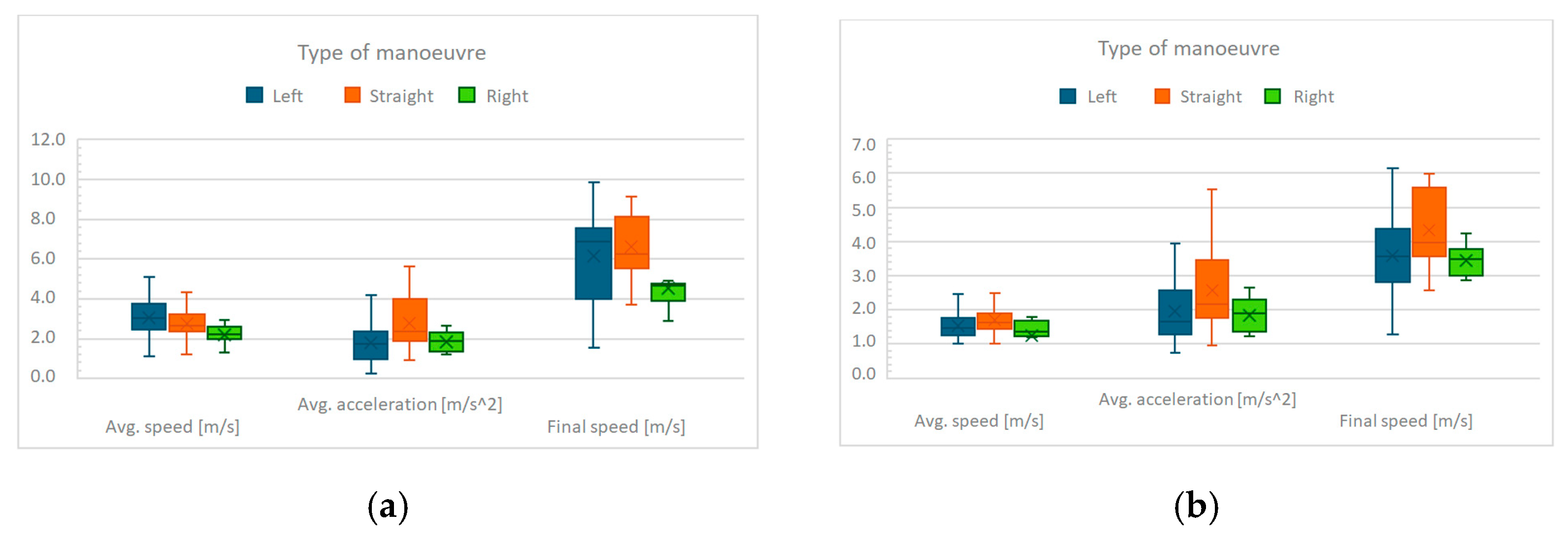
Figure 1 shows the boxplots related to the average acceleration, average speed, and exit speed of electric vehicles for the three maneuvers considered (left turn, right turn, and crossing). Specifically, Figure 2a displays the data for the complete maneuvers, thus involving different distances traveled (6 m for the right turn, 7 m for crossing, and 12 m for the left turn). In contrast, Figure 2b presents the same results normalized over a uniform traveled distance of 3 m for each maneuver.

Table 1 and

Table 2. Average values of acceleration and speed, final speeds, 1st and 3rd quartiles for BEVs, with different distances traveled.

	Left	Straight	Right
	(Q1–Q3)	(Q1–Q3)	(Q1–Q3)
Avg. Speed [m/s]	3.06 (3.72–2.47)	2.76 (3.23–2.37)	2.19 (2.58–2.00)
Avg. Acceleration [m/s2]	1.79 (2.35–0.95)	2.78 (3.97–1.90)	1.86 (2.41–1.39)
Final Speed [m/s]	6.15 (7.53–3.97)	6.61 (8.13–5.52)	4.53 (4.77–3.87)

report the numerical values for the same experimental sets. As can be observed from Figure 2a and Table 2, the highest final speed is reached for the straight crossing maneuver, even though the distance traveled is not the longest. When comparing the turning maneuvers, it can be noted that the average acceleration during a left turn is slightly lower than that of a right turn. The most dispersed data are those related to the left turn, which is understandable given the urban intersection context and the higher level of uncertainty associated with vehicle flow conflicts for this maneuver. By considering a uniform traveled distance (3 m, Figure 2b and

Table 3. Average values of acceleration and speed, final speeds, 1st and 3rd quartiles for BEVs, with uniform distances traveled (3 m).

	Left	Straight	Right
	(Q1–Q3)	(Q1–Q3)	(Q1–Q3)
Avg. Speed [m/s]	1.54 (1.76–1.26)	1.70 (1.89–1.43)	1.25 (1.70–1.23)
Avg. Acceleration [m/s2]	1.97 (2.57–1.29)	2.58 (3.46–1.76)	1.82 (2.32–1.31)
Final Speed [m/s]	3.59 (4.37–2.82)	4.33 (5.57–3.58)	3.45 (3.78–3.00)

), the differences between the various maneuvers can be compared more accurately: in this case, as well, the straight crossing results as the fastest. As for the turns, the highest average acceleration is observed in the left-turn maneuver, since the turning radius is lower than that of the right turn, having a stronger influence on the driver’s driving dynamics. The peak values for electric vehicles observed here are significantly higher than those documented in earlier literature, such as the study by Choi and Kim [17], who found mean acceleration values around 2.07 m/s².

4.1.2. HEV and ICE Vehicles

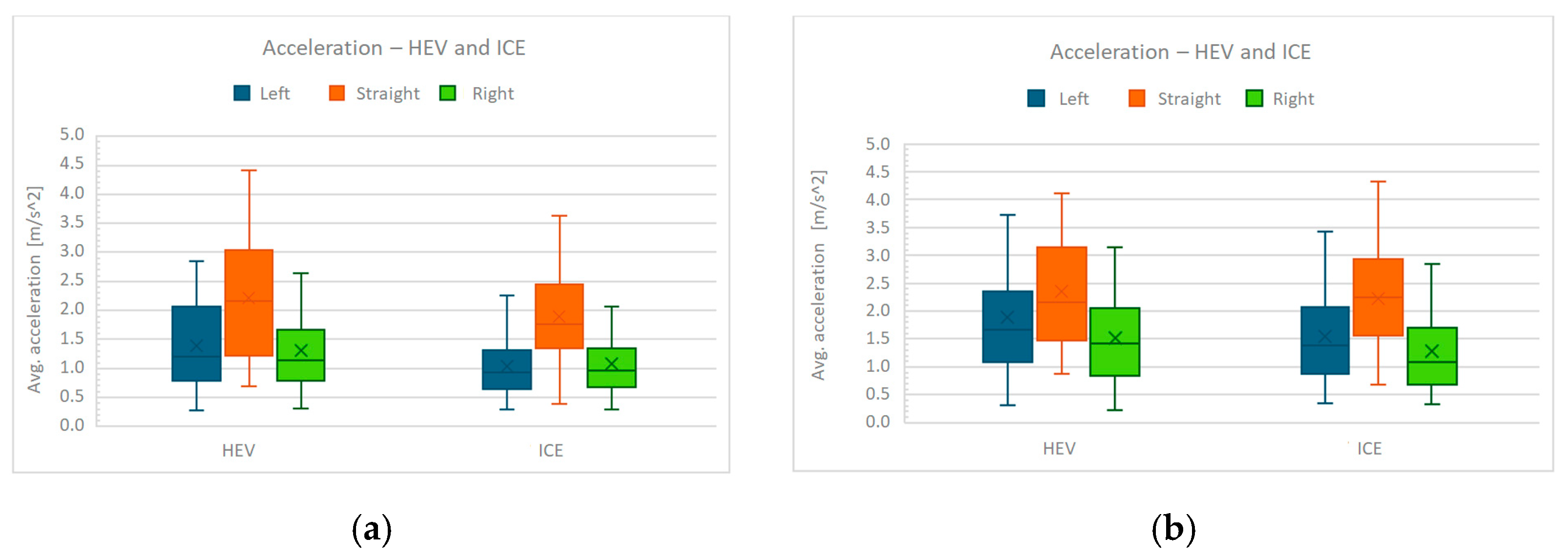
The same analyses were carried out, under the same test conditions, for hybrid vehicles (HEVs) and internal combustion engine vehicles (ICE). Initially, the average acceleration values for hybrid and internal combustion engine vehicles were compared for each maneuver, considering both the actual distances traveled and the uniform distance of 3 m (Figure 3). As can be observed, the average acceleration values are not significantly different, and in light of this result, hybrid and internal combustion engine vehicles are treated as a single sample in the following analyses.

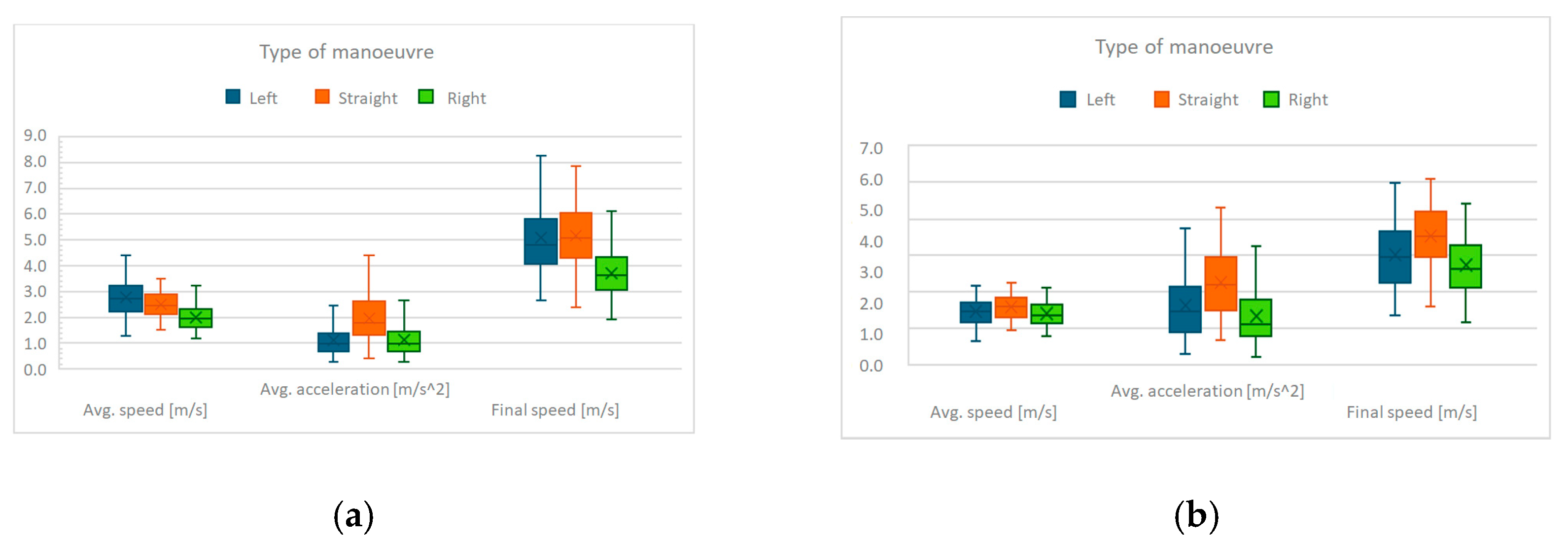
Figure 4 shows, as previously, the boxplots related to the average acceleration, average speed, and final speed of HEVs and ICE vehicles for the three maneuvers considered. Figure 4a displays the data for the complete maneuvers, while Figure 4b presents the same results normalized over a uniform traveled distance of 3 m.

Table 4. Average values of acceleration and speed, final speeds, 1st and 3rd quartiles for HEVs and ICE vehicles, with different distances traveled.

	Left	Straight	Right
	(Q1–Q3)	(Q1–Q3)	(Q1–Q3)
Avg. Speed [m/s]	2.79 (3.24–2.22)	2.50 (2.89–2.10)	2.01 (2.33–1.63)
Avg. Acceleration [m/s2]	1.12 (1.39–0.67)	1.97 (2.62–1.33)	1.13 (1.47–0.69)
Final Speed [m/s]	5.10 (5.82–4.07)	5.18 (6.04–4.30)	3.72 (4.33–3.07)

and

Table 5. Average values of acceleration and speed, final speeds, 1st and 3rd quartiles for HEVs and ICE vehicles, with uniform distances traveled (3 m).

	Left	Straight	Right
	(Q1–Q3)	(Q1–Q3)	(Q1–Q3)
Avg. Speed [m/s]	1.47 (1.73–1.17)	1.59 (1.84–1.31)	1.41 (1.65–1.14)
Avg. Acceleration [m/s2]	1.63 (2.16–0.88)	2.26 (2.94–1.49)	1.34 (1.77–0.78)
Final Speed [m/s]	3.00 (3.64–2.24)	3.53 (4.19–2.96)	2.73 (3.28–2.13)

report the numerical values for the same experimental sets. It can be observed that for hybrid and internal combustion engine vehicles, as for electric ones, the straight crossing maneuver is the fastest, followed by the left turn, and lastly by the right turn maneuver. It is also observed that the acceleration values recorded for HEVs and ICE vehicles are, on average, lower than those obtained under similar conditions for BEVs; this also affects the final speed from the respective maneuvers, which are consistently higher for electric vehicles. Furthermore, there is a greater dispersion in the acceleration data for BEV vehicles, likely attributable to drivers’ lower familiarity with these types of vehicles and the resulting greater heterogeneity in driving behavior.

These values align with and extend previous studies. For example, Rakha et al. [20] and Murro [25] reported acceleration ranges for ICE vehicles between 1.5 and 2.5 m/s² during straight crossing maneuvers, which closely match the present findings.

The observed BEV advantage in our study supports outcomes from Zhang et al. [22] and Huang et al. [23], who highlight the role of instantaneous torque in enhancing electric vehicle responsiveness. The final speed values corroborate the acceleration results and provide a metric for evaluating intersection clearance times. Compared to Murro [25], who reported final speeds below 30 km/h for most vehicle types, this study captures the more agile performance of modern BEVs. The sharp performance gain for BEVs highlights the need to update gap acceptance models, particularly in simulations and infrastructure design, which have often been based on outdated ICE vehicle dynamics only.

Statistical comparisons confirmed that BEVs achieved significantly higher mean accelerations than ICE and HEV vehicles (

Table 6. Statistical comparison of mean longitudinal acceleration between BEVs and conventional vehicles (ICE + HEV) during all maneuvers. Values include 95% confidence intervals, effect sizes (Cohen’s d), and results from non-parametric Wilcoxon tests (with Cliff’s Δ as a measure of effect magnitude).

Group Comparison	Mean Diff. (m/s2)	95% CI (Diff.)	p-Value	Cohen’s d	Wilcoxon p	$\mathbf{Cliff}’\mathbf{s} ∆$
BEV vs. ICE/HEV (straight)	0.95	[0.75–1.15]	<0.001	0.80	<0.001	0.73 (large)
BEV vs. ICE/HEV (left turn)	0.66	[0.41–0.89]	0.002	0.63	0.003	0.61 (moderate)
BEV vs. ICE/HEV (right turn)	0.54	[0.29–0.79]	0.005	0.57	0.006	0.55 (moderate)

). The effect size was large for all pairwise comparisons, indicating a substantial practical difference. To control the false discovery rate under multiple testing, the Benjamini–Hochberg correction (q = 0.05) was applied. For variables showing non-normal distributions, Wilcoxon rank-sum tests and Cliff’s delta were also calculated, confirming the robustness of all findings.

4.2. Mathematical Modeling of Acceleration

To describe the acceleration dynamics more precisely, several classes of mathematical models were applied to each maneuver category: a fourth-degree polynomial, modeling acceleration, and velocity as continuous functions of time; the Akçelik acceleration model and the arctangent function, continuously modeling smoothed velocity growth over time. The three models were selected for their complementary properties: 4th-degree polynomials for flexibility and widespread use in microsimulation, the Akçelik model for its asymmetric acceleration profile embedded in traffic analysis tools such as SIDRA, and the arctangent function for its bounded velocity and realistic bell-shaped acceleration, consistent with ICE/HEV/BEV propulsion dynamics. All the models were calibrated separately for ICE, HEV, and BEV vehicles.

The fourth-degree polynomial function has the form:

$$a\left(t\right)=\alpha t^4+\beta t^3+\gamma t^2+\delta t+ϵ$$

(1)

The Akçelik acceleration model is expressed by the equation:

$$a\left(t\right)={r·a}_m·{\theta }^n{\left(1-{\theta }^m\right)}^2$$

(2)

where: $\theta ={\displaystyle \frac{t}{t_m}}$, $a_m$ is the maximum acceleration, $t_m$ is the time necessary to reach the final speed, $r$, $m$ and $n$ are parameters to be determined.

The arctangent velocity model [26] models the velocity as an arctangent function of time:

$$v\left(t\right)=\vartheta ·arctan\left(\tau t+\sigma \right)+\epsilon$$

(3)

where: $\vartheta ,$ $\sigma$ and $\tau$ are parameters to be calibrated and $\epsilon =\vartheta ·arctan\left(\sigma \right)$ since $v\left(0\right)=0$.

Table 7. List of symbols used in mathematical models.

Symbol	Description	Source/Meaning
$a\left(t\right)$	Instantaneous longitudinal acceleration [m/s2]	Derived from MEMS accelerometer
$v\left(t\right)$	Longitudinal speed [m/s]	RTK-GPS validated
$s\left(t\right)$	Traveled distance [m]	Numerical integration of acceleration
$a_m$	Maximum acceleration	Estimated from empirical data
$v_{max}$	Maximum (exit) speed	Observed final speed for each maneuver
$t_0$	Initial time (start of maneuver)	Defined at signal green/standstill
$t_m$	Time necessary to reach the final speed	Estimated from empirical data
$\vartheta ,\tau ,\sigma$	Parameters in arctangent function	Calibration parameters
$r, m, n$	Parameters in Akçelik acceleration model	Calibration parameters
$\alpha ,\beta ,\gamma ,\delta$	Parameters in fourth-degree polynomial acceleration model	Calibration parameters

contains a list of the symbols and parameters adopted in the considered mathematical models.

The calibration of all models was conducted under explicit physical constraints. Time-related parameters (e.g., $t_m$) and scale factors were restricted to positive values to ensure realistic, monotonic growth of velocity. Polynomial coefficients were inspected to avoid non-physical oscillations and preserve a single acceleration peak. The Akçelik and arctangent parameters were bounded within empirically observed ranges of acceleration and speed.

For practical applications, polynomial functions provide high flexibility for descriptive analyses but may lead to overfitting and should not be used for extrapolation. Akçelik models are recommended for traffic microsimulation environments, whereas arctangent functions are particularly suitable for trajectory-based modeling and autonomous vehicle motion planning, due to their smooth and bounded behavior.

All models were required to satisfy physical boundary conditions. For velocity-based models, initial conditions were set to $v\left(0\right)=0$, with monotonic increase until reaching the asymptotic exit speed $v_{max}$. For acceleration-based models, the initial condition was $a\left(0\right)\ge 0$, with strictly non-negative accelerations during the rising phase. To avoid non-physical solutions, parameter constraints were applied $v_{max}\ge 0$, $\tau >0$ and scale factors positive. These constraints ensured that fitted functions preserved the expected kinematic behavior.

4.2.1. Straight Crossing Maneuver

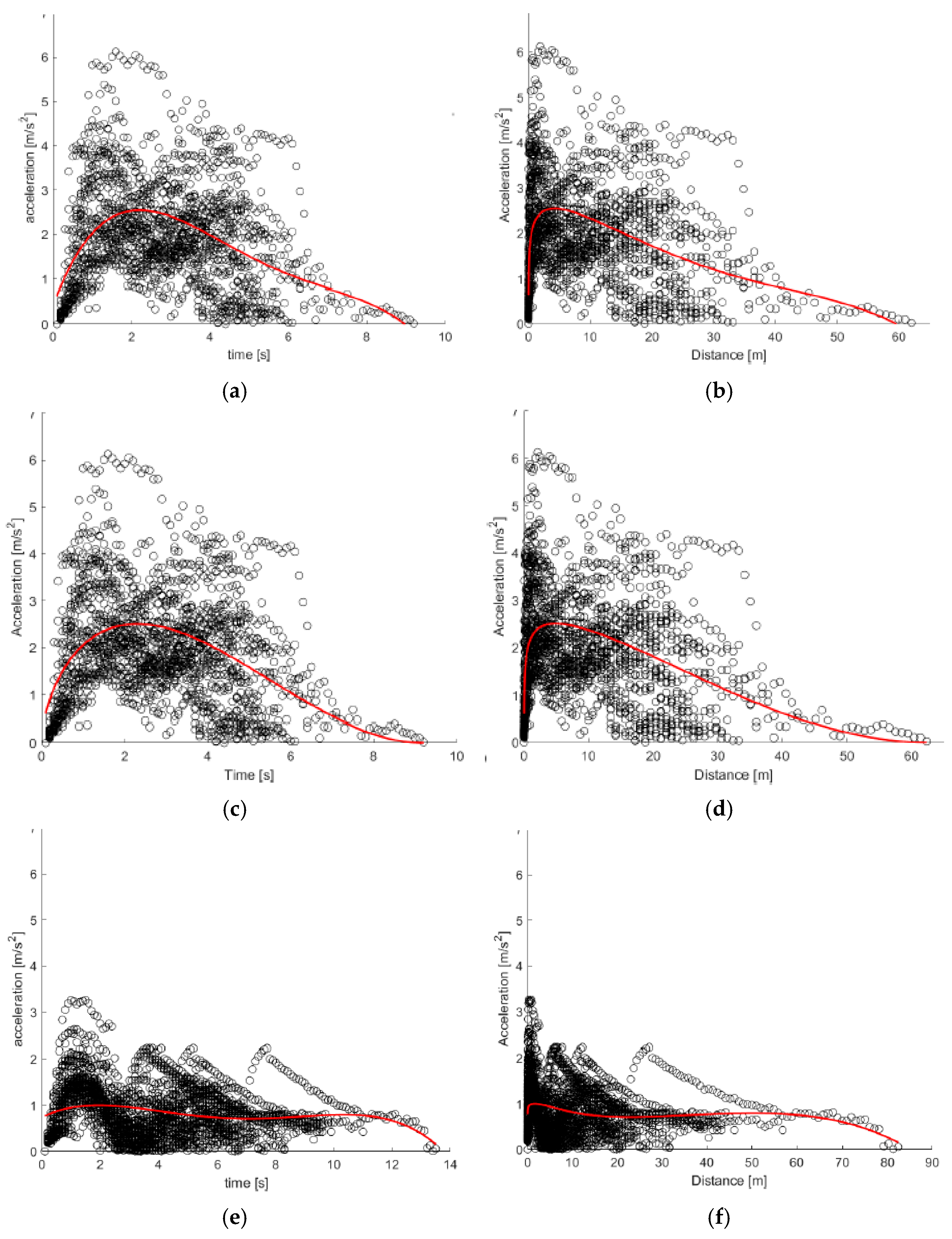
This maneuver displayed the most aggressive acceleration profiles, especially for BEVs.

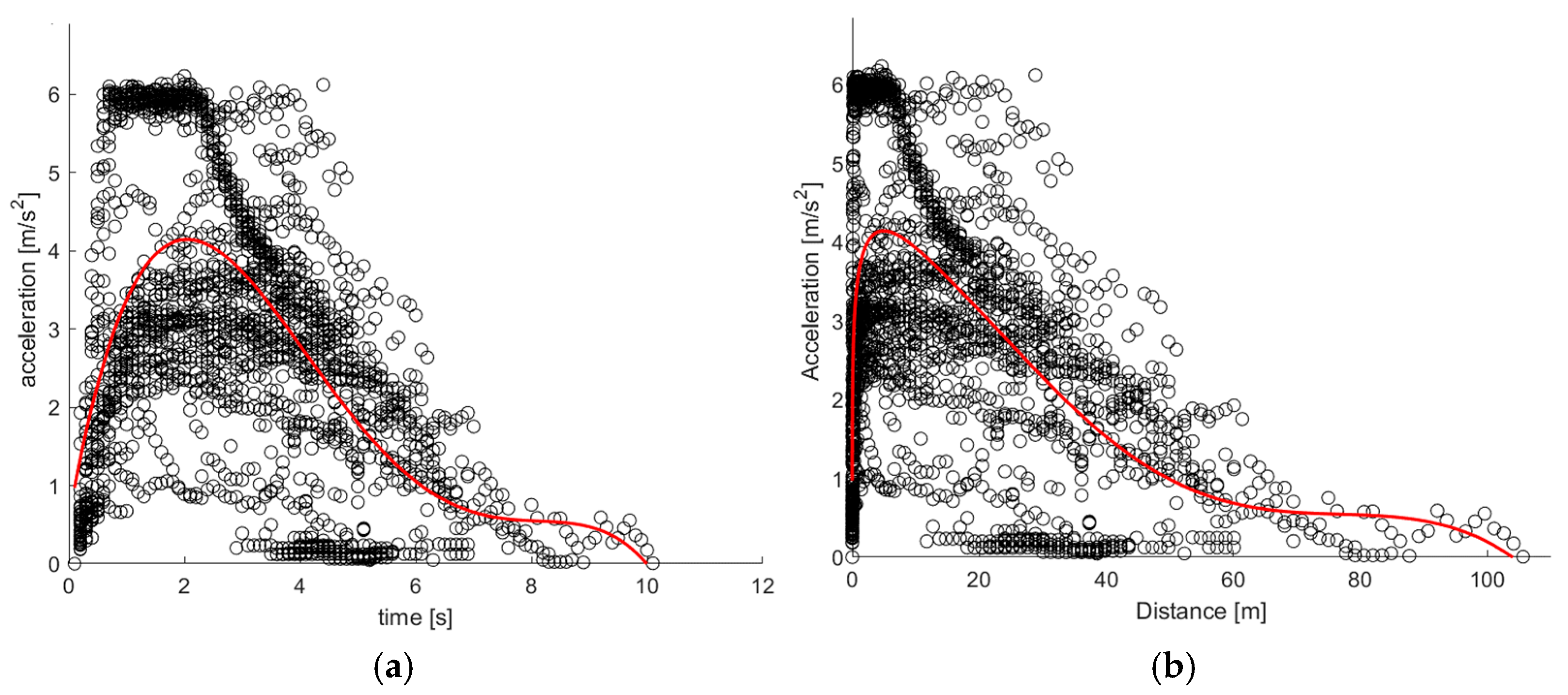
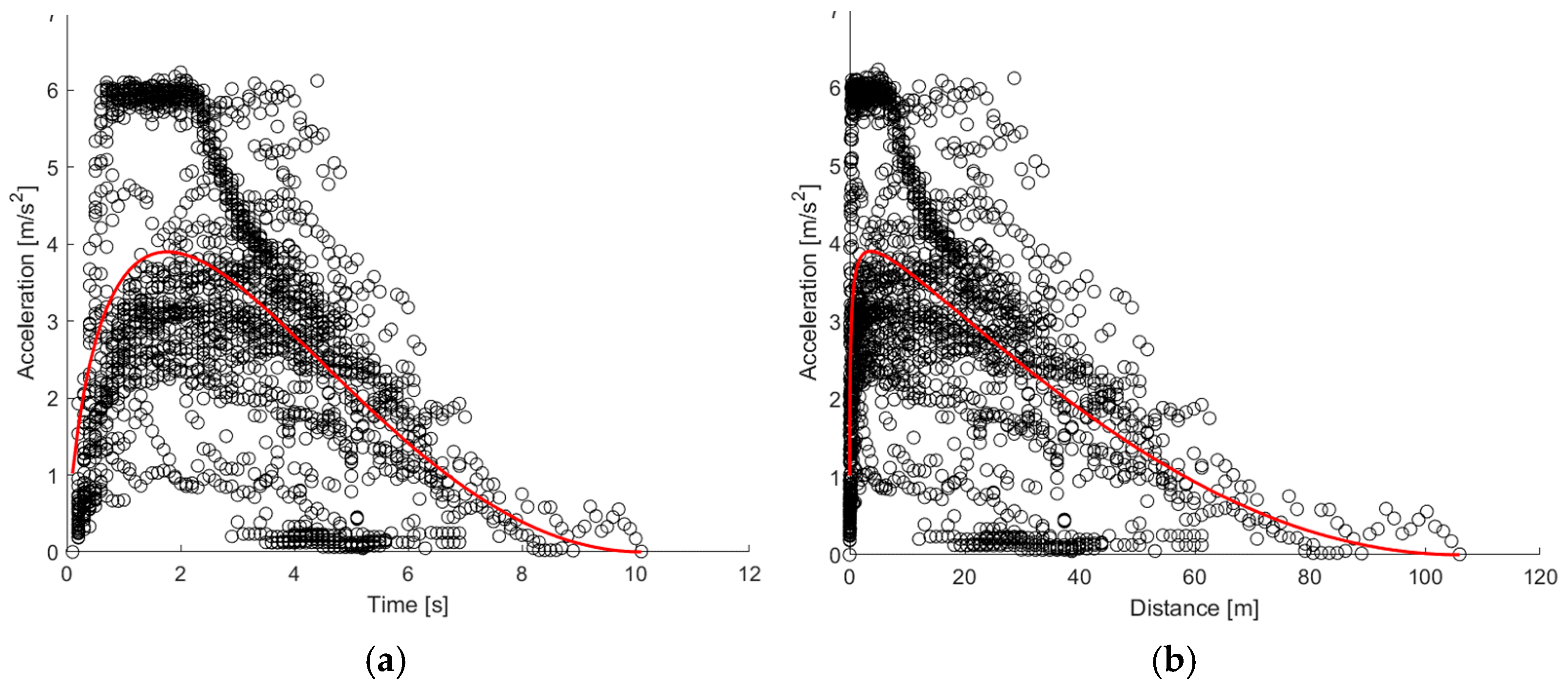
Figure 5 and Figure 6 show, respectively, the polynomial and Akçelik curves fitting acceleration over time and distance for the crossing maneuver of electric vehicles. The calibrated models are:

$${a\left(t\right)}_{polyn}=-0.00759t^4+0.185t^3-1.516t^2+4.135t+0.575$$

(4)

$${MSE}_{polyn}=0.0916$$

$${a\left(t\right)}_{Akcelik}=800·4.138·{\vartheta }^{1.094}·{\left(1-{\vartheta }^{0.0529}\right)}^2$$

(5)

$${MSE}_{Akcelik}=0.0931$$

Acceleration-time curves exhibit a sharp rise and a distinct peak around 1.5–2 s, indicating a strong and immediate initial acceleration, consistent with the high torque of electric drivetrains. Both models demonstrate excellent overlap with the empirical data, with minimal error throughout the time and space domains.

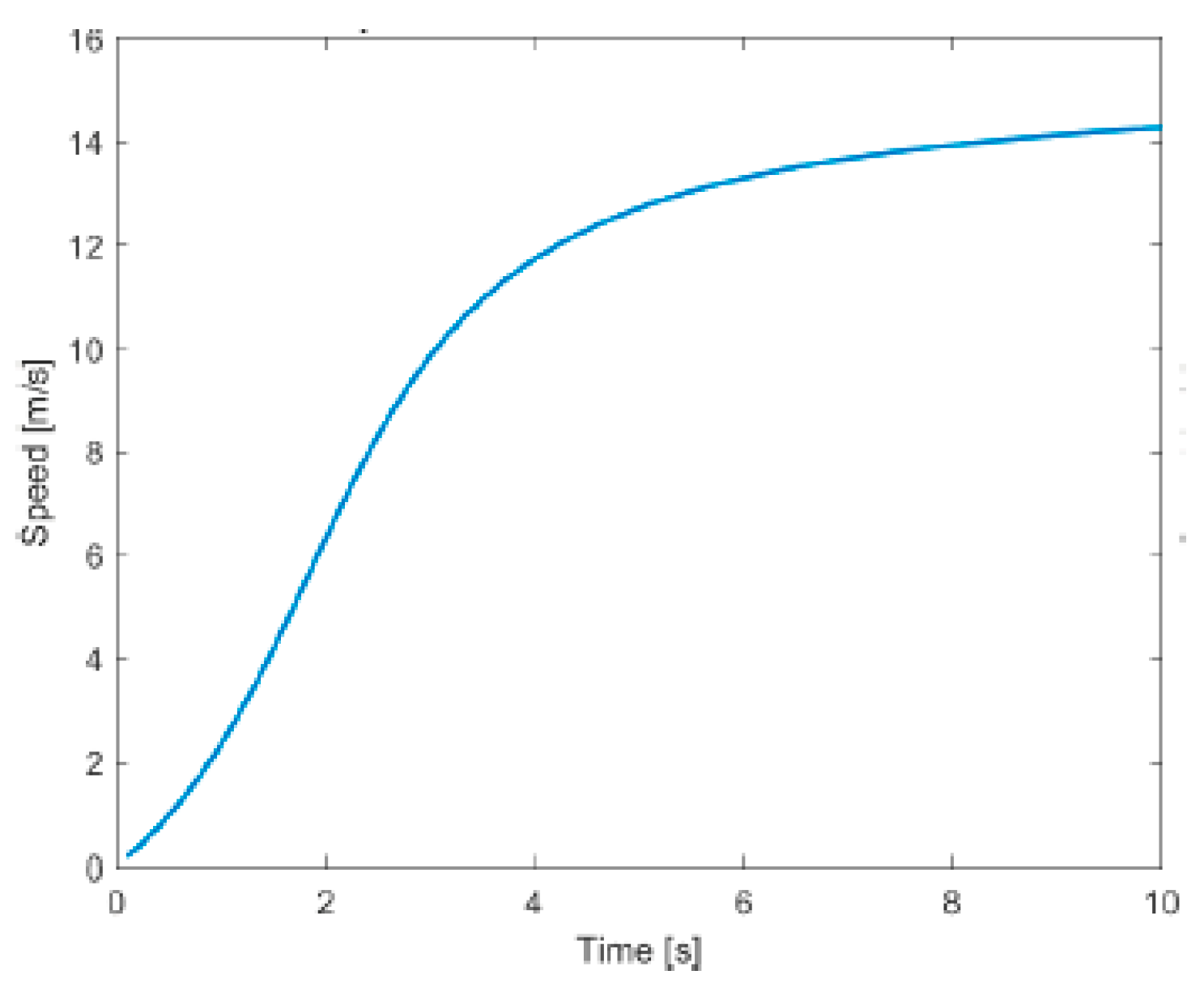
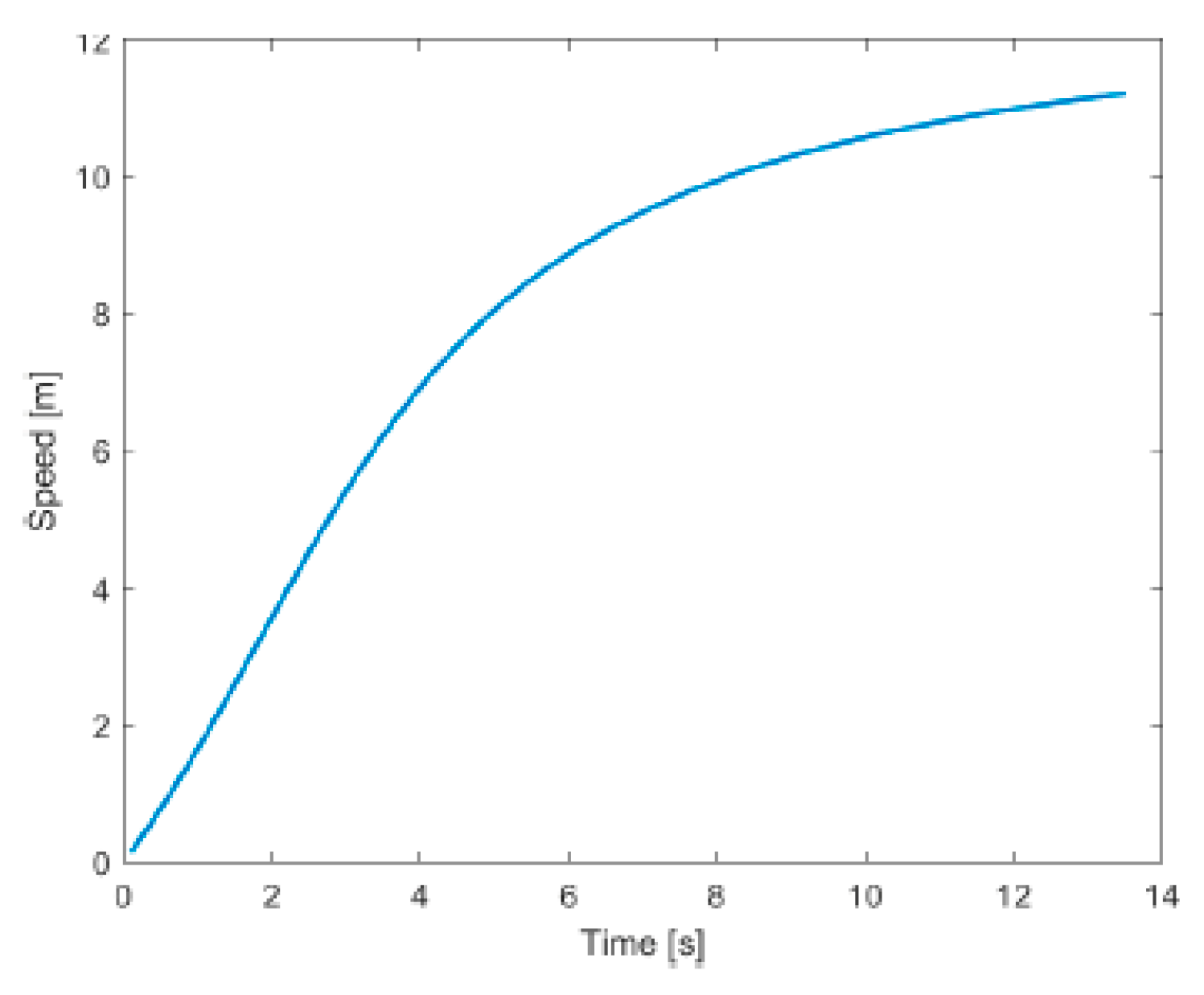
Concerning speed over time, BEVs show a noticeably steeper slope in the first few seconds, with a rapid transition to a plateau. This reflects the fast initial speed gain observed in the experimental data. The arctangent model successfully reproduces the nonlinear acceleration-to-velocity transition (Figure 7) and captures the asymptotic behavior at higher speeds:

$${v\left(t\right)}_{arctan}=-6.191·arctan\left(-0.699t+1.108\right)+5.18$$

(6)

$${MSE}_{acrtan}=0.2068$$

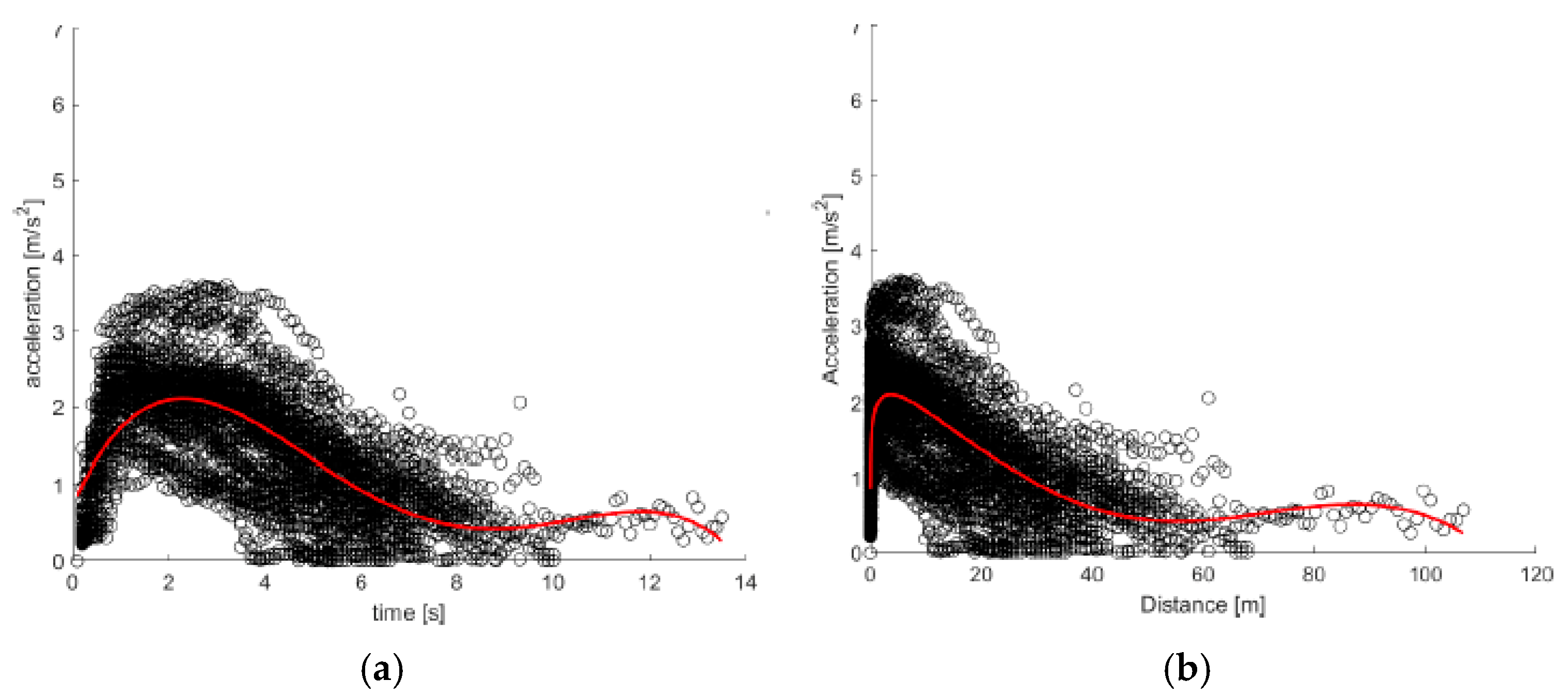
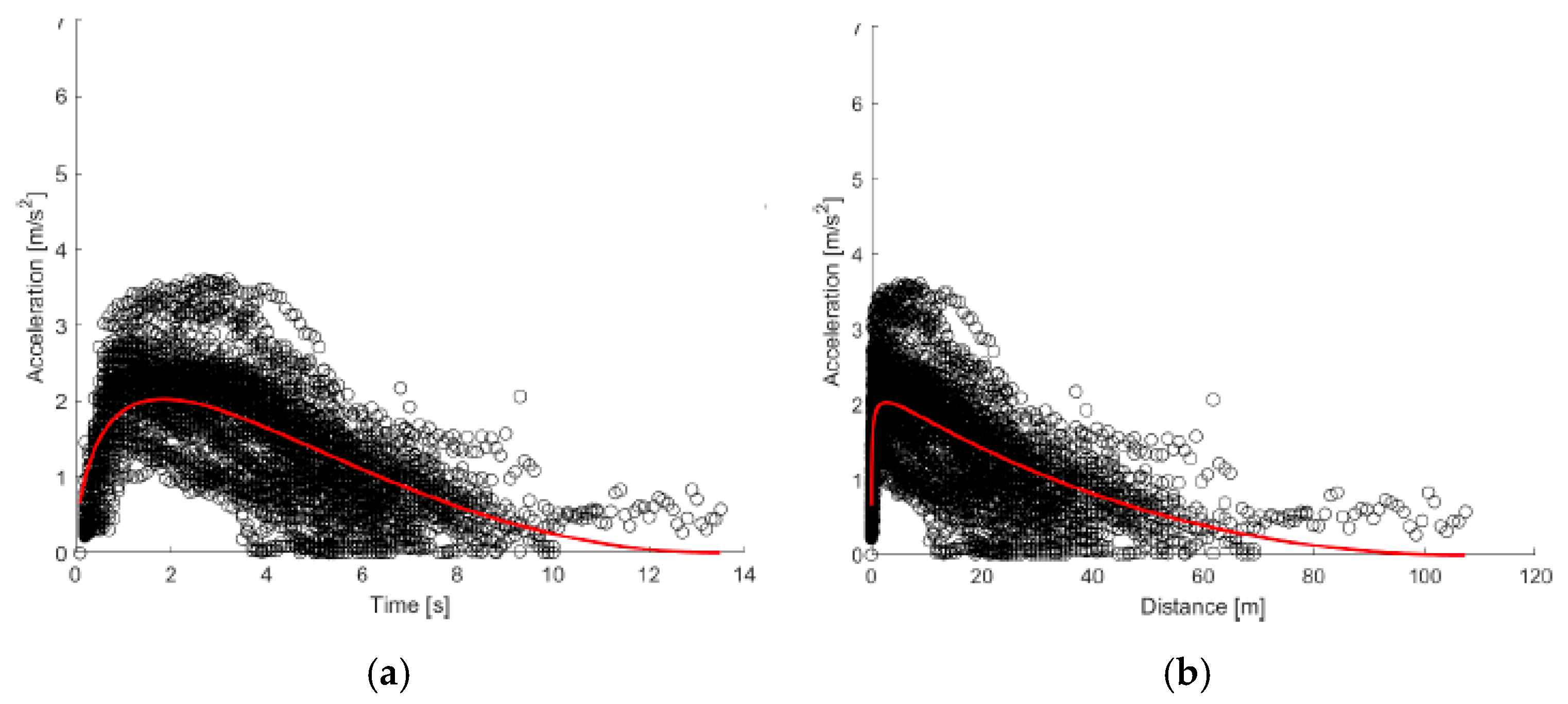
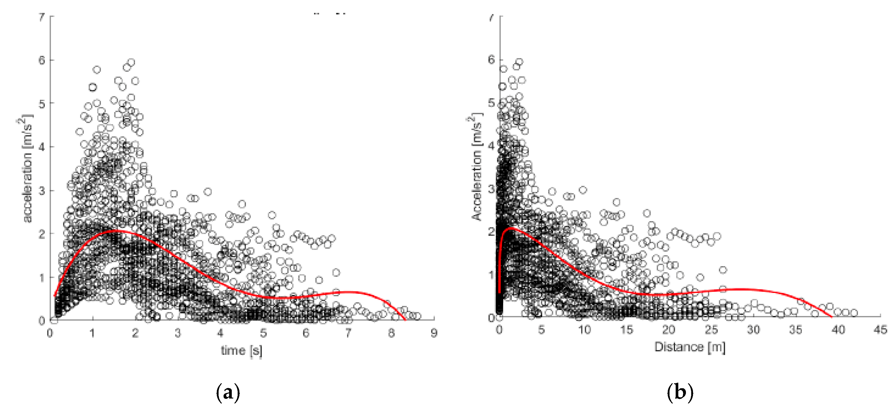
As regards HEV vehicles, they show smoother, more gradual curves, reaching lower peaks at later times (around 2.5–3 s). In this case, the cloud of instantaneous acceleration dots appears more compact compared to BEVs (see Figure 8 and Figure 9). This phenomenon can be explained by the impact of the hybrid powertrain on driving behavior: it is less powerful than that of an electric car but faster than an internal combustion engine, providing instantaneous support to propulsion. In fact, the graphs in Figure 8 show a white area with no data points during the first few seconds of the maneuver, as observed in the previous case, indicating that the increase in acceleration is almost immediate, thanks to the electric assistance, rather than gradual, as will be observed later for the combustion engine vehicle.

The calibrated models for HEVs are:

$${a\left(t\right)}_{polyn}=-0.00149t^4+0.0456t^3-0.451t^2+1.422t+0.717$$

(7)

$${MSE}_{polyn}=0.0351$$

$${a\left(t\right)}_{Akcelik}=688·2.098·{\vartheta }^{0.957}·{\left(1-{\vartheta }^{0.0497}\right)}^2$$

(8)

$${MSE}_{Akcelik}=0.0866$$

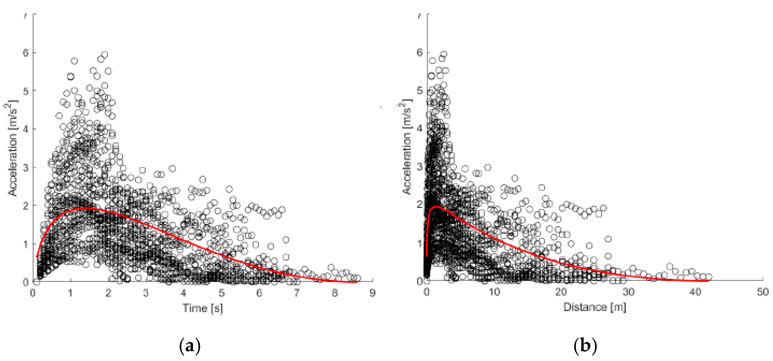
The polynomial function exhibits a marked overfitting phenomenon that leads to an increase in speed at the end of the test. With the Akçelik function, this phenomenon disappears, and the trend of acceleration as a function of space and time aligns with the literature. As for the MSE, it is lower for the polynomial function as a consequence of overfitting; for the Akçelik function, it is slightly higher but still acceptable.

The peak acceleration (2 m/s²) was found to be approximately 50% lower than that of BEVs (4 m/s²). As for speed over time (Figure 10), HEVs velocity curves are more gradual, with an extended mid-phase compared with BEVs, showing slower acceleration over time. The calibrated arctangent model is:

$${v\left(t\right)}_{arctan}=6.122·arctan\left(0.318t-0.579\right)+3.21$$

(9)

$${MSE}_{acrtan}=0.1675$$

Finally, the ICE vehicles are analyzed, which, as previously mentioned, show a less steep increasing trend compared to BEVs and HEVs; however, with peak values of comparable magnitude. As can be seen from Figure 11 and Figure 12, the scatter plot is less dense and the acceleration increases gradually, leaving small empty areas in the initial moments of the test.

Focusing on the mathematical models, also in this case, the Akçelik model does not exhibit overfitting and presents an MSE slightly higher than that of the polynomial function, but still acceptable. In detail, the calibrated models for ICE vehicles are:

$${a\left(t\right)}_{polyn}=-0.0115t^4+0.214t^3-1.314t^2+2.710t+0.296$$

(10)

$${MSE}_{polyn}=0.0675$$

$${a\left(t\right)}_{Akcelik}=997·2.475·{\vartheta }^{1.057}·{\left(1-{\vartheta }^{0.416}\right)}^2$$

(11)

$${MSE}_{Akcelik}=0.104$$

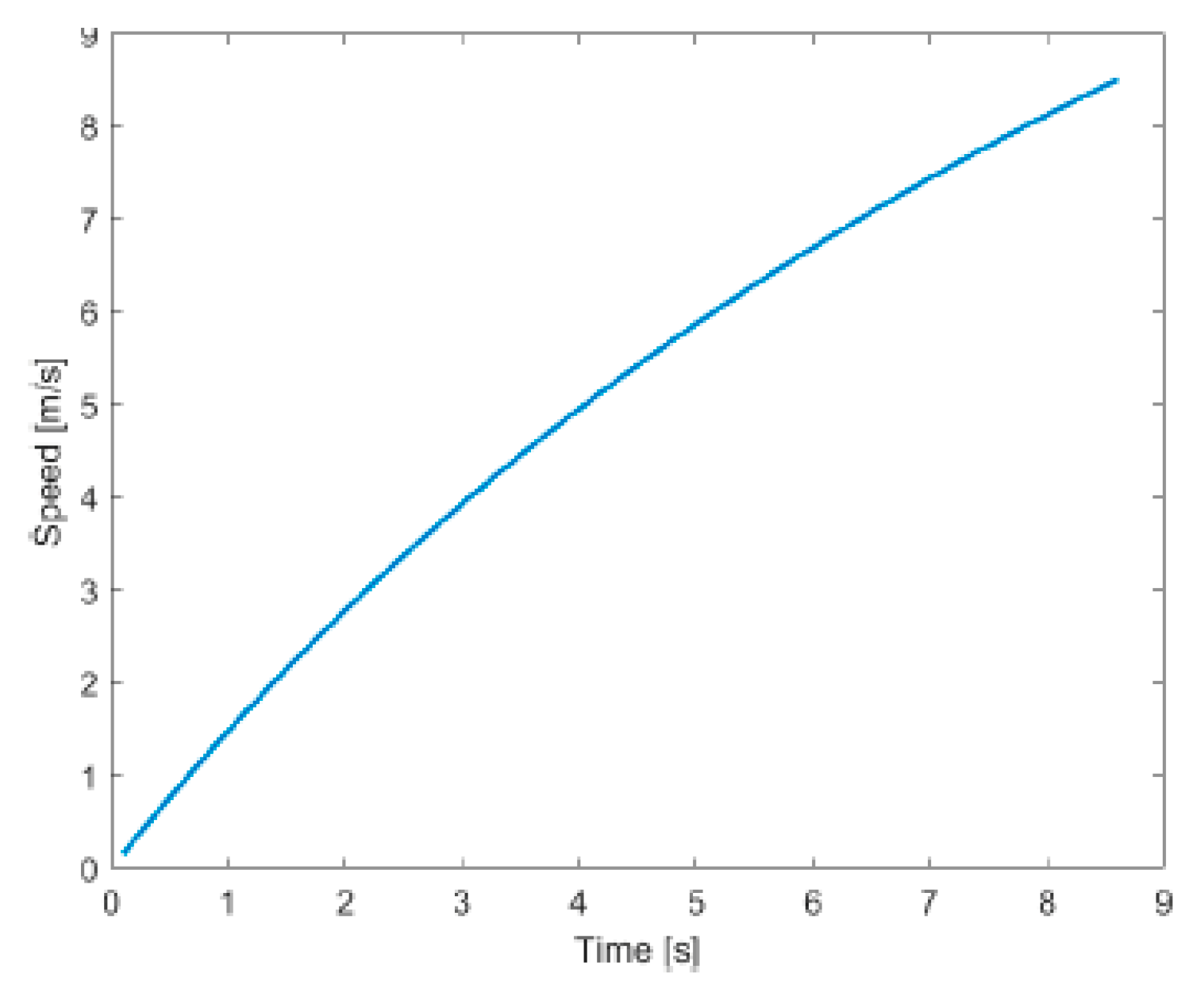
In this case, the arctangent function also effectively describes the trend of speed as a function of time (Figure 13), with a more gradual progression, consistent with this type of powertrain.

In

Table 8. Summary of model fit for each powertrain—straight crossing maneuver.

Maneuver	Powertrain	Polynomial	Akçelik	Arctangent
		(MSE)	(MSE)	(MSE)
Straight	BEV	0.0916	0.0931	0.2068
	HEV	0.0351	0.0866	0.1675
	ICE	0.0675	0.104	0.2832

, a summary of model fit for each powertrain and straight crossing maneuver is provided.

4.2.2. Left and Right Turn Maneuvers

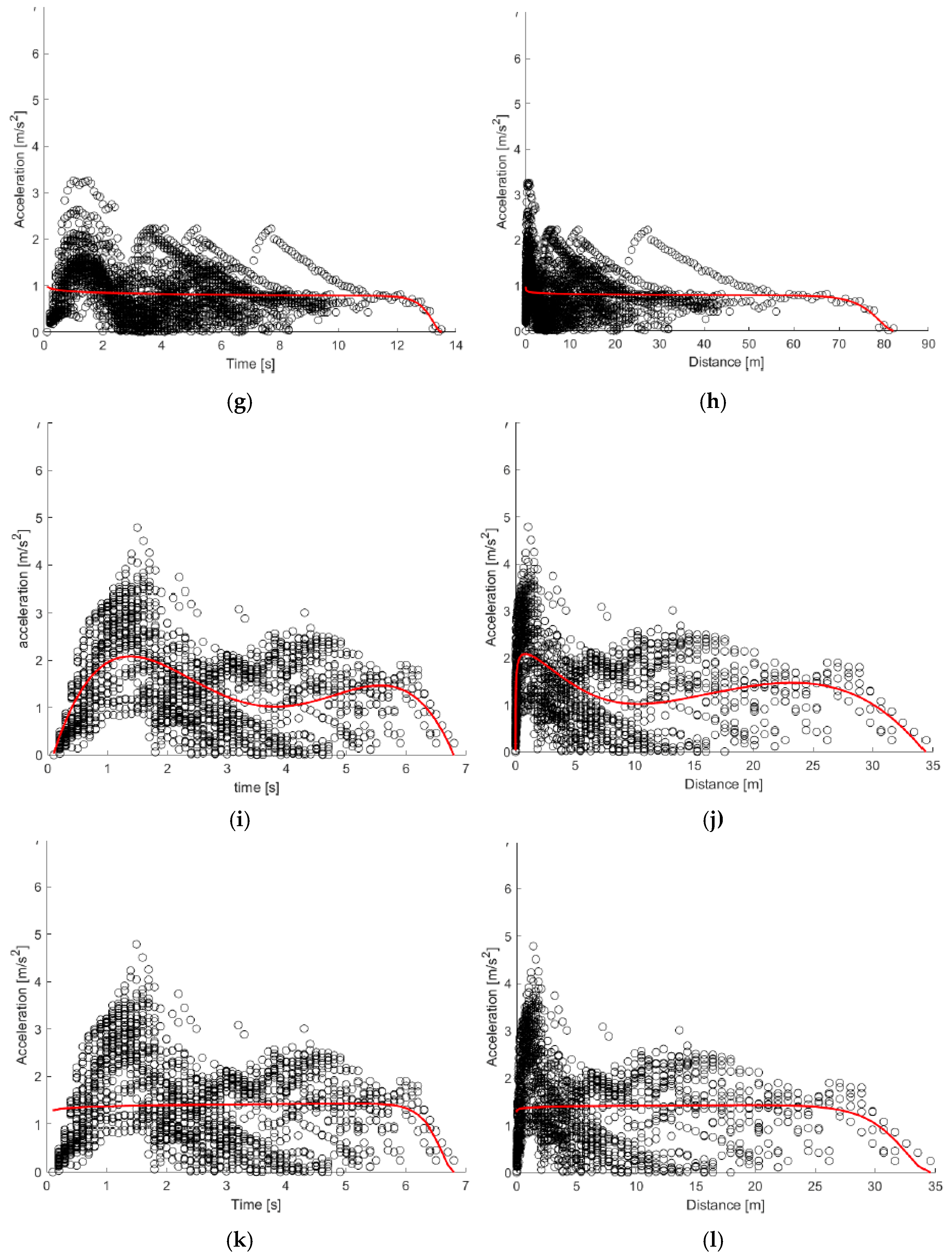
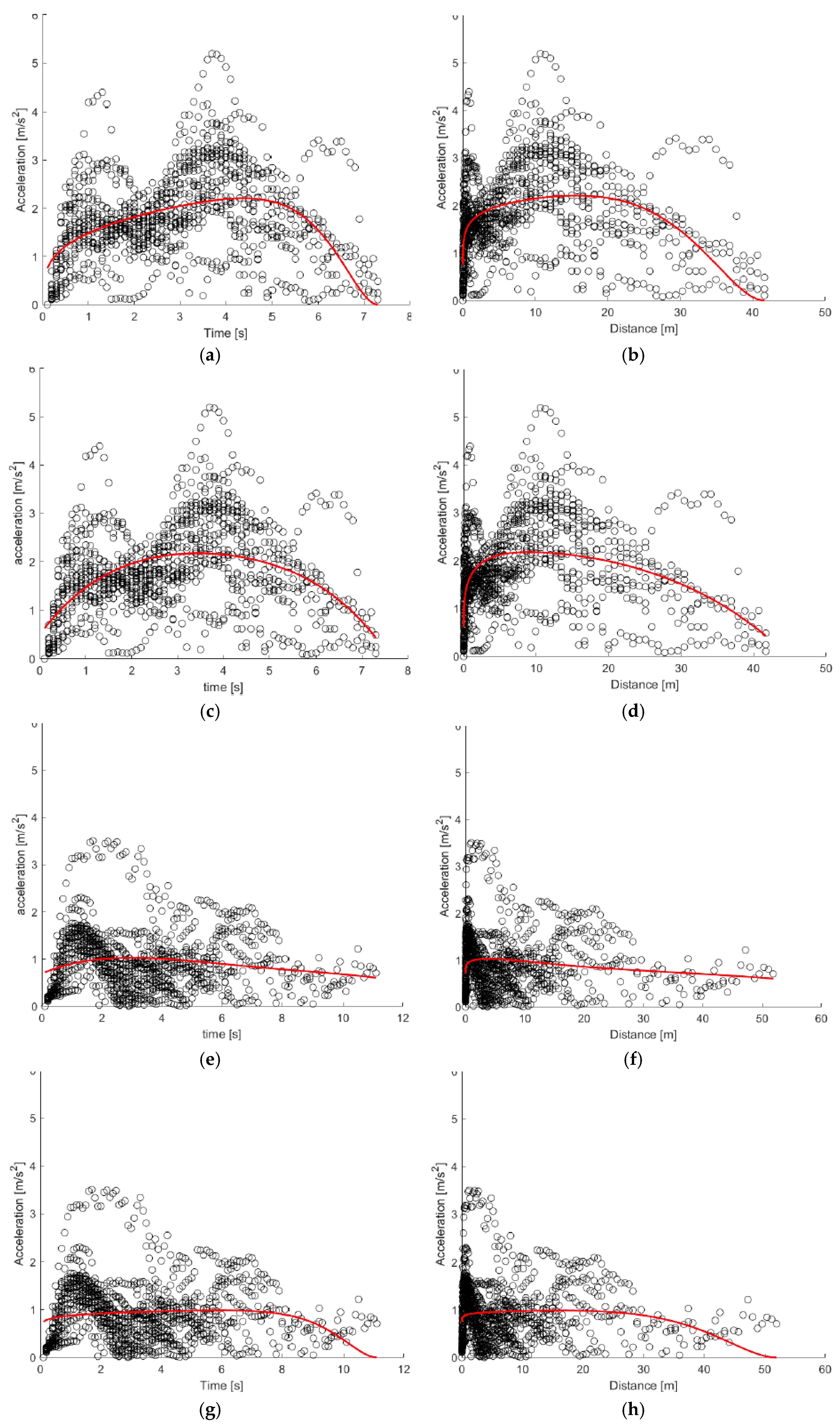
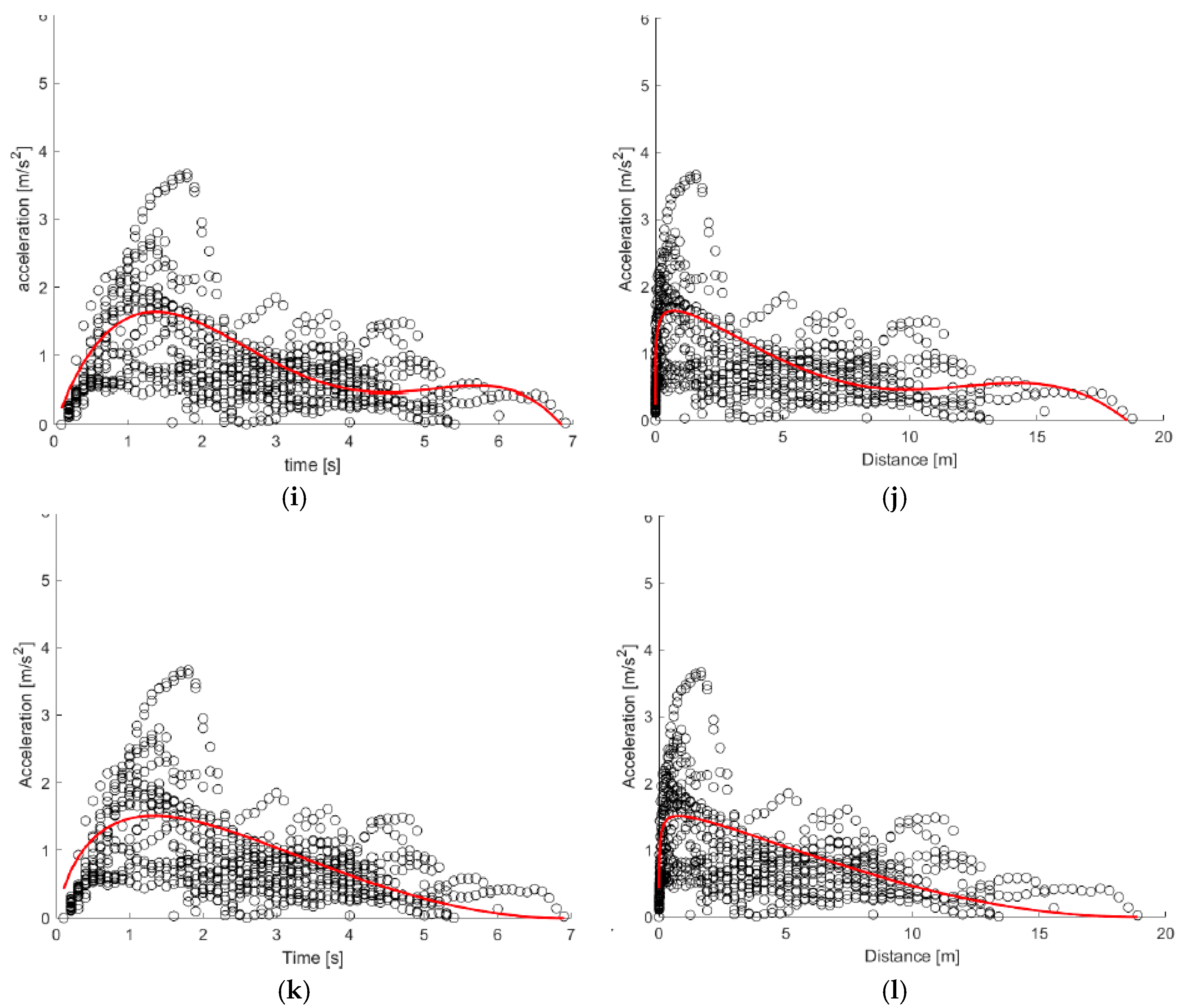
The left turn and right turn maneuvers are characterized by greater irregularity both across individual trials and among different vehicle types. The scatter plots (Figure 14 and Figure 15) reveal a high degree of heterogeneity: in some trials, the acceleration peak is reached almost instantaneously, while in others it takes several seconds. This variability in behavior is primarily influenced by the fluctuating intensity of urban traffic. The following of this section presents the equation of the fourth-degree polynomial and Akcelic models, for acceleration (Table 5, Table 6 and Table 7), and the arctangent function for speed. Also in the case of these maneuvers, a substantial difference is observed between the models, which can be partially attributed to overfitting, as previously discussed.

BEVs exhibit high peak accelerations, which represent the maximum values for the maneuver type but remain lower than those observed during longitudinal crossing. The point clouds and the curves derived from the models reveal a smoother acceleration profile, with lower peak values compared to the previous maneuver (Figure 14). Both the polynomial model and Akçelik model accurately capture the general acceleration trends over time for both left and right turns (

Table 9. Polynomial and Akçelik calibrated models for left and right turn maneuvers, BEVs.

		BEVs
Polynomial	Left turn Right turn	$a\left(t\right)=-0.00462t^4+0.1047t^3-0.8344t^2+2.353t+0.407$ ${MSE}_{polyn}=0.0854$ $a\left(t\right)=-0.003t^4+0.0462t^3-0.3515t^2+1.272t+0.504$ ${MSE}_{polyn}=0.1003$
Akçelik	Left turn Right turn	$a\left(t\right)=3.271·2.822·{\vartheta }^{0.599}·{\left(1-{\vartheta }^{-1.13}\right)}^2$ ${MSE}_{Akcelik}=0.089$ $a\left(t\right)=0.96·2.775·{\vartheta }^{15.92}·{\left(1-{\vartheta }^{-7.81}\right)}^2$ ${MSE}_{Akcelik}=0.1419$

,

Table 10. Polynomial and Akçelik calibrated models for left and right turn maneuvers, HEVs.

		HEVs
Polynomial	Left turn Right turn	$a\left(t\right)=-0.000357t^4+0.0097t^3-0.0843t^2+0.228t+0.791$ ${MSE}_{polyn}=0.0456$ $a\left(t\right)=-0.000223t^4+0.0067t^3-0.0718t^2+0.273t+0.696$ ${MSE}_{polyn}=0.083$
Akçelik	Left turn Right turn	$a\left(t\right)=0.495·1.518·{\vartheta }^{-0.0598}·{\left(1-{\vartheta }^{266.4}\right)}^2$ ${MSE}_{Akcelik}=0.056$ $a\left(t\right)=0.685·1.52·{\vartheta }^{0.0704}·{\left(1-{\vartheta }^{8.765}\right)}^2$ ${MSE}_{Akcelik}=0.1146$

and

Table 11. Polynomial and Akçelik calibrated models for left and right turn maneuvers, ICE vehicles.

		ICE
Polynomial	Left turn Right turn	$a\left(t\right)=-0.0376t^4+0.5397t^3-2.5707t^2+4.408t-0.385$ ${MSE}_{polyn}=0.0929$ $a\left(t\right)=-0.0211t^4+0.3246t^3-1.6655t^2+2.953t-0.0421$ ${MSE}_{polyn}=0.0604$
Akçelik	Left turn Right turn	$a\left(t\right)=0.531·2.706·{\vartheta }^{0.0267}·{\left(1-{\vartheta }^{26.26}\right)}^2$ ${MSE}_{Akcelik}=0.2582$ $a\left(t\right)=735.2·2.186·{\vartheta }^{1.164}·{\left(1-{\vartheta }^{0.0506}\right)}^2$ ${MSE}_{Akcelik}=0.0953$

), showing low mean square errors. However, the Akçelik model proves to be slightly less precise.

In the case of HEVs, left-turn maneuvers yield two particularly distinct models for both the polynomial and Akçelik curves (Figure 14g,h). The nearly constant acceleration profile is attributed to the high variability within the sample: unlike longitudinal crossings, where the peak acceleration typically occurs within the first few seconds after departure, the peak values here are more evenly distributed across the entire duration of the maneuver. A similar pattern is observed for right-turn maneuvers as well (Figure 15).

For ICE vehicles, substantial variability is also present across individual trials, particularly in left-turn maneuvers. This heterogeneity negatively affects the performance of the Akçelik model, which displays a relatively high MSE, exceeding that of the other calibrated models and especially greater than that of the polynomial model.

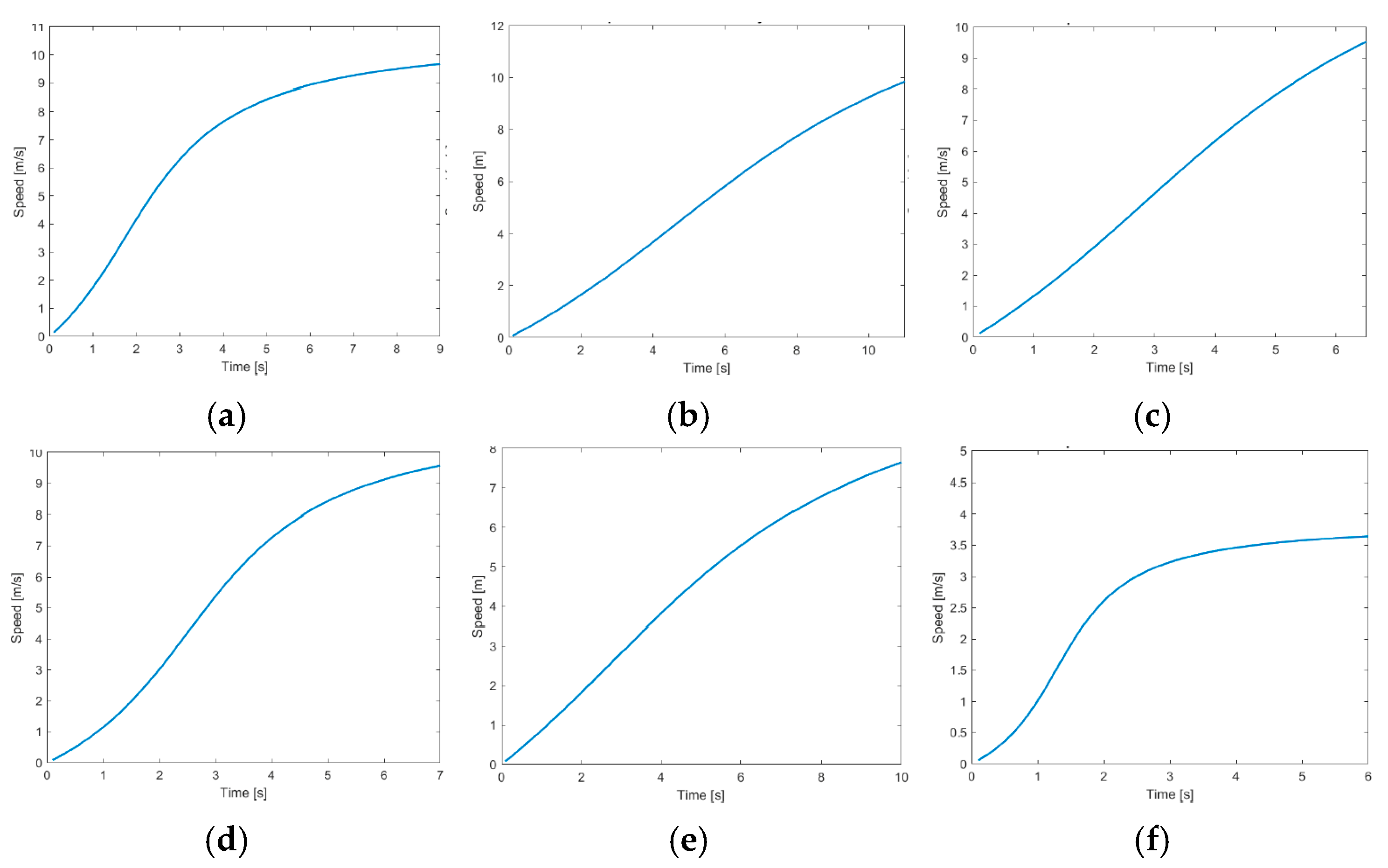
Regarding the speed profile over time (Figure 15 and

Table 12. Arctangent calibrated models for $v\left(t\right)$, left and right turn maneuvers, all vehicle types.

		Arctangent Model
BEVs	Left turn Right turn	$v\left(t\right)=4.65·arctan\left(0.541t-0.944\right)+3.52$ ${MSE}_{arctan}=0.0889$ $v\left(t\right)=4.56·arctan\left(0.528t-1.326\right)+4.21$ ${MSE}_{arctan}=0.0311$
HEVs	Left turn Right turn	$v\left(t\right)=7.035·arctan\left(0.154t-0.721\right)+4.39$ ${MSE}_{arctan}=0.1012$ $v\left(t\right)=5.428·arctan\left(0.1868t-0.512\right)+2.57$ ${MSE}_{arctan}=0.0511$
ICE	Left turn	$v\left(t\right)=7.074·arctan\left(0.247t-0.694\right)+4.29$ ${MSE}_{arctan}=0.0997$
	Right turn	$v\left(t\right)=1.518·arctan\left(1.22t-1.571\right)+1.52$ ${MSE}_{arctan}=0.0144$

), in the case of left-turn maneuvers, the curve described by the arctangent function for battery electric vehicles (BEVs) tends to flatten in the final seconds, approaching a horizontal asymptote that can be interpreted as the regime speed. When compared to the longitudinal crossing maneuver, the left turn is markedly slower and exhibits a more gradual acceleration phase. A similar, albeit less pronounced, trend is also observed in right-turn maneuvers.

For hybrid electric vehicles (HEVs), the speed profile does not show significant variations, except in the initial phase where the arctangent function captures a slower acceleration rate (Figure 16b,e).

Finally, for internal combustion engine (ICE) vehicles, the speed profile during left turns appears regular and closely similar to that of HEVs. However, in the case of right turns, the profile diverges significantly, displaying a shape more like that of electric vehicles (Figure 16c,f).

In

Table 13. Summary of model fit for each powertrain—left/right turn maneuvers.

Maneuver	Powertrain	Polynomial	Akçelik	Arctangent
		(MSE)	(MSE)	(MSE)
Right turn	BEV	0.1003	0.1419	0.0311
	HEV	0.083	0.1146	0.0511
	ICE	0.0604	0.0953	0.0144
Left turn	BEV	0.0854	0.089	0.0889
	HEV	0.0456	0.056	0.1012
	ICE	0.0929	0.2582	0.0997

, a summary of model fit for each powertrain and left/right turn maneuvers is provided.

5. Discussion and Conclusions

The findings presented in this study underscore significant variations in vehicle acceleration behavior across propulsion systems and maneuver types, with important implications for traffic engineering, autonomous driving systems design, road safety analysis and forensic engineering. Battery Electric Vehicles consistently demonstrated superior acceleration performance in tested scenarios, particularly during straight crossings, where their instantaneous torque delivery enabled sharper velocity gains within the initial seconds of motion. This confirms prior observations in the literature yet provides more granular evidence through high-frequency empirical data. The increased variability observed in BEV acceleration translates into potentially more unpredictable driving dynamics for other road users or autonomous vehicle perception systems. This data dispersion can be directly attributed to the high sensitivity of the accelerator pedal and the non-linear power delivery curve characteristic of electric vehicles, which often necessitates greater calibration and adaptation from the driver. Consequently, driving behaviors may range from extremely aggressive (fully leveraging the vehicle’s maximum performance) to excessively cautious (due to apprehension of abrupt acceleration). Such inherent variability, if not adequately managed, could potentially lead to increased stress on infrastructure elements or erroneous perceptions by pedestrians and other vehicles, thereby impacting overall road safety. These findings underscore the importance of driver training programs or Advanced Driver-Assistance Systems (ADAS) capable of modulating the powertrain response based on the driver’s individual driving style. Conversely, Hybrid Electric Vehicles and Internal Combustion Engine vehicles exhibited more homogeneous profiles, with HEVs slightly outperforming ICEs in initial acceleration due to electric assistance.

Analyses revealed that, across all propulsion types, right-turn maneuvers are associated with lower average accelerations, a trend primarily attributable to the geometric constraints imposed by the typically tighter curve radius and the necessity of maintaining a controlled speed for both safety and comfort. Left turns exhibit greater dispersion in acceleration profiles. This variability is attributable not only to geometric constraints but also significantly to the driver’s behavioral constraints. The increased number of conflict points with other vehicular flows, coupled with variable expectations regarding the behavior of other road users, introduces a high degree of uncertainty in the acceleration decision. This circumstance has direct implications for road safety, raising the potential risk of accidents involving vulnerable users such as pedestrians and cyclists, who may not adequately predict vehicle acceleration dynamics and, consequently, maneuver times.

Furthermore, in intersection design, uniform assumptions about vehicle dynamics can lead to suboptimal signal timing and gap acceptance policies. These policies may either underestimate BEVs’ capacity to merge into traffic flow or, conversely, create unrealistic expectations for ICE vehicle drivers, resulting in more frequent conflict situations if ADAS and AV systems do not account for the heterogeneous vehicle fleet composition. Moreover, it should be noted that although the dataset includes drivers of different age groups and genders, as well as tests performed under varying traffic conditions, the effects of these variables were not systematically analyzed due to limited sample sizes. Future research should explicitly incorporate driver characteristics (age, gender) and environmental factors (e.g., weather, lighting, pavement conditions) into the modeling framework, as they are likely to influence acceleration and driving strategies.

The arctangent function proved particularly adept at capturing velocity evolution across maneuvers, offering a smooth, realistic transition from standstill to cruising speed that can be effectively utilized by autonomous vehicles for more accurate trajectory prediction of other vehicles, thus mitigating false positives and unnecessary evasive actions. The same function can be used to render the behavior of autonomous vehicles more “human-like” and predictable, both in terms of acceleration and transitions between acceleration and steady-state speed, thereby facilitating their safe integration into mixed traffic environments. Although the polynomial and Akçelik models provided good fits, the latter struggled to replicate the aggressive initial acceleration of BEVs, underscoring the need to refine classical models in light of evolving vehicle technologies.

These results not only validate the relevance of maneuver- and vehicle-specific modeling in simulation environments but also offer validated parameters for improving the fidelity of crash reconstructions in electrifying urban settings. In fact, beyond traffic modeling, these findings hold significant implications for forensic engineering and accident reconstruction. Accurate, empirically derived acceleration profiles are essential for reconstructing pre-crash vehicle behavior, especially where acceleration from rest plays a key role in collision causality. The study provides high-resolution benchmark data that can improve estimates of speeds achieved and timing sequences at intersections, factors critical to both legal and insurance determinations. Traditional reconstruction methods often rely on idealized or generalized acceleration assumptions, which this research shows to be insufficient for modern vehicle fleets. By offering vehicle- and manoeuvre-specific profiles grounded in real-world measurements, this work enhances the precision and reliability of forensic analyses in cases involving intersection crashes. In practical terms, the findings contribute to policy and regulation by providing data suitable for the calibration of traffic signal timings in accordance with heterogeneous vehicle fleets, for the refinement of ADAS algorithms in line with UNECE regulatory requirements, to improve traffic microsimulation tools by replacing constant-acceleration assumptions with empirically validated curves, and for the design of sustainable urban intersections consistent with EU mobility strategies. In addition to the already discussed behavioral variability, road surface conditions (e.g., asphalt roughness, wet vs. dry pavement) and weather factors (temperature and humidity) can also influence tire grip and, consequently, acceleration capability. Driver heterogeneity, including experience and individual driving style, may further contribute to the dispersion of acceleration profiles observed across maneuvers.

The study has several limitations that need to be acknowledged. First, the test sample is geographically limited to Italian contexts, where the distinct characteristics of the local traffic rules and regional driving behaviors can lead to variations in the execution modalities of maneuvers compared to other international contexts; broader international experimental campaigns could validate the generalizability of the findings. Second, combined maneuvers (e.g., lane changes during longitudinal acceleration) were not considered due to the limited number of real cases. Finally, environmental variables (such as road surface condition, weather, and lighting) and socio-demographic variables (such as age and gender) were not systematically analyzed; nonetheless, they remain a noteworthy topic for further research.

References

- World Health Organization. Global Status Report on Road Safety 2023: Country and Territory Profiles. 2024. Available online: https://iris.who.int/handle/10665/379826 (accessed on 16 August 2025).
- EU Road Safety Policy Framework 2021–2030—Next Steps Towards “Vision Zero”. 19 June 2019. Available online: https://transport.ec.europa.eu/system/files/2021-10/SWD2190283.pdf (accessed on 16 August 2025).
- International Traffic Safety Data and Analysis Group. Available online: https://www.itf-oecd.org/road-safety-annual-report-2022 (accessed on 16 August 2025).
- ISTAT (2025). Incidenti Stradali in Italia—2024. Available online: https://www.istat.it/wp-content/uploads/2025/07/REPORT_INCIDENTI_STRADALI_2024.pdf (accessed on 16 August 2025).
- Micucci, A.; Mantecchini, L.; Sangermano, M. Analysis of the relationship between turning signal detection and motorcycle driver’s characteristics on urban roads; A case study. Sensors 2019, 19, 1802. [Google Scholar] [CrossRef]
- Barth, M.; Boriboonsomsin, K. Real-world carbon dioxide impacts of traffic congestion. Transp. Res. Rec. 2008, 2058, 163–171. [Google Scholar] [CrossRef]
- Abdulmawjoud, A.A.; Jamel, M.G.; Al-Taei, A.A. Traffic flow parameters development modelling at traffic calming measures located on arterial roads. Ain Shams Eng. J. 2021, 12, 437–444. [Google Scholar] [CrossRef]
- Paden, B.; Čáp, M.; Yong, S.Z.; Yershov, D.; Frazzoli, E. A survey of motion planning and control techniques for self-driving urban vehicles. IEEE Trans. Intell. Veh. 2016, 1, 33–55. [Google Scholar] [CrossRef]
- Narayanan, S.; Chaniotakis, E.; Antoniou, C. Factors affecting traffic flow efficiency implications of connected and autonomous vehicles: A review and policy recommendations. Adv. Transp. Policy Plan. 2020, 5, 1–50. [Google Scholar]
- Fambro, D.B.; Fitzpatrick, K.; Koppa, R. Determination of Stopping Sight Distances; Transportation Research Board: Washington, DC, USA, 1997; Volume 400. [Google Scholar]
- Vangi, D.; Begani, F.; Spitzhüttl, F.; Gulino, M.S. Vehicle accident reconstruction by a reduced order impact model. Forensic Sci. Int. 2019, 298, 426-e1–426-e11. [Google Scholar] [CrossRef]
- Akçelik, R.; Biggs, D.C. Acceleration profile models for vehicles in road traffic. Transp. Sci. 1987, 21, 36–54. [Google Scholar] [CrossRef]
- Wang, J.; Dixon, K.K.; Li, H.; Ogle, J. Normal acceleration behavior of passenger vehicles starting from rest at all-way stop-controlled intersections. Transp. Res. Rec. 2004, 1883, 158–166. [Google Scholar] [CrossRef]
- Dabbour, E.; Easa, S.M.; Dabbour, O. Minimum lengths of acceleration lanes based on actual driver behavior and vehicle capabilities. J. Transp. Eng. Part A Syst. 2021, 147, 04020162. [Google Scholar] [CrossRef]
- Dabbour, E.; Easa, S.M. Revised method for calculating departure sight distance at two-way stop-controlled (TWSC) intersections. Transp. Res. Rec. 2021, 2675, 904–914. [Google Scholar] [CrossRef]
- Zhang, Z.; Dong, Y.; Han, Y. Dynamic and control of electric vehicle in regenerative braking for driving safety and energy conservation. J. Vib. Eng. Technol. 2020, 8, 179–197. [Google Scholar] [CrossRef]
- Choi, E.; Kim, E. Critical aggressive acceleration values and models for fuel consumption when starting and driving a passenger car running on LPG. Int. J. Sustain. Transp. 2017, 11, 395–405. [Google Scholar] [CrossRef]
- Mondal, S.; Gupta, A. Evaluation of driver acceleration/deceleration behavior at signalized intersections using vehicle trajectory data. Transp. Lett. 2023, 15, 350–362. [Google Scholar] [CrossRef]
- Li, Z.; Pan, S.; Mao, K.; Xu, Y. Combined acceleration slip regulation for multi-wheel distributed electric drive vehicles considering torque loss factor. Control. Eng. Pract. 2024, 146, 105893. [Google Scholar] [CrossRef]
- Rakha, H.; Snare, M.; Dion, F. Vehicle dynamics model for estimating maximum light-duty vehicle acceleration levels. Transp. Res. Rec. 2004, 1883, 40–49. [Google Scholar] [CrossRef]
- Haas, R.; Inman, V.; Dixson, A.; Warren, D. Use of intelligent transportation system data to determine driver deceleration and acceleration behavior. Transp. Res. Rec. 2004, 1899, 3–10. [Google Scholar] [CrossRef]
- Zhang, L.; Cai, X. Control strategy of regenerative braking system in electric vehicles. Energy Procedia 2018, 152, 496–501. [Google Scholar] [CrossRef]
- Huang, Y.; Yu, H.; Yin, J.; Hu, H.; Bai, S.; Meng, X.; Wang, M. An integrated approach for the energy-efficient driving strategy optimization of multiple trains by considering regenerative braking. Comput. Ind. Eng. 2018, 126, 399–409. [Google Scholar] [CrossRef]
- Murro, A. Valori Accelerometrici Dei Veicoli in Immissione Nelle Intersezioni. ASAIS: Associazione per lo Studio e l’Analisi Degli Incidenti Stradali, Proceeding of the 2006 Conference. 1, pp. 1–48. Available online: http://www.asais.it/it/downloadtree.asp?filecode=2845 (accessed on 14 October 2025).
- Li, T.; Kovaceva, J.; Dozza, M. Modeling collision avoidance maneuvers for micromobility vehicles. J. Saf. Res. 2023, 87, 232–243. [Google Scholar] [CrossRef] [PubMed]
- Della Mura, M.; Failla, S.; Gori, N.; Micucci, A.; Paganelli, F. E-Scooter Presence in Urban Areas: Are Consistent Rules, Paying Attention and Smooth Infrastructure Enough for Safety? Sustainability 2022, 14, 14303. [Google Scholar] [CrossRef]
- Şentürk Berktaş, E.; Tanyel, S. Effect of autonomous vehicles on performance of signalized intersections. J. Transp. Eng. Part A Syst. 2020, 146, 04019061. [Google Scholar] [CrossRef]
- Rakha, H.; Ding, Y. Impact of stops on vehicle fuel consumption and emissions. J. Transp. Eng. 2003, 129, 23–32. [Google Scholar] [CrossRef]
- Brach, R.M.; Brach, R.M.; Pongetti, K. Analysis of high-speed sideswipe collisions using data from small overlap tests. SAE Int. J. Transp. Saf. 2014, 2, 86–99. [Google Scholar] [CrossRef][Green Version]
- Jia, C.; Liu, W.; He, H.; Chau, K.T. Superior energy management for fuel cell vehicles guided by improved DDPG algorithm: Integrating driving intention speed prediction and health-aware control. Appl. Energy 2025, 394, 126195. [Google Scholar] [CrossRef]
Figure 1.
Sensitivity analysis of the Savitzky–Golay filtering procedure applied to a synthetic acceleration signal with a sharp transient peak.
Figure 2.
Average acceleration and speed for BEVs. (a) data obtained from complete maneuvers; (b) data normalized over uniform distances (3 m). Boxplots show median, interquartile range, and whiskers at 1.5 × IQR. Sample size: BEV n = 296.
Figure 3.
Average acceleration of HEV and ICE vehicles: (a) data obtained from complete maneuvers; (b) data normalized over uniform distances (3 m). Boxplots show median, interquartile range, and whiskers at 1.5 × IQR. Sample sizes: HEV n = 319; ICE n = 99.
Figure 4.
Average acceleration and speed for HEVs and ICE vehicles. (a) data obtained from complete maneuvers; (b) data normalized over uniform distances (3 m).
Figure 5.
Acceleration over time (a) and distance (b) for crossing maneuver—BEVs (black dots are experimentally observed values and the red line is the calibrated polynomial curve).
Figure 6.
Acceleration over time (a) and distance (b) for crossing maneuver—BEVs (black dots are experimentally observed values and the red line is the calibrated Akçelik curve).
Figure 7.
Speed over time for crossing maneuver—calibrated arctangent models for BEVs.
Figure 8.
Acceleration over time (a) and distance (b) for crossing maneuver—HEVs (black dots are experimentally observed values and the red line is the calibrated polynomial curve).
Figure 9.
Acceleration over time (a) and distance (b) for crossing maneuver—HEVs (black dots are experimentally observed values and the red line is the calibrated Akçelik curve).
Figure 10.
Speed over time for crossing maneuver—calibrated arctangent models for HEVs.
Figure 11.
Acceleration over time (a) and distance (b) for crossing maneuver—ICE vehicles (black dots are experimentally observed values and the red line is the calibrated polynomial curve).
Figure 12.
Acceleration over time (a) and distance (b) for crossing maneuver—ICE vehicles (black dots are experimentally observed values and the red line is the calibrated Akçelik curve).
Figure 13.
Speed over time for crossing maneuver—calibrated arctangent models for ICE vehicles.
Figure 14.
Acceleration over time and distance for left turn maneuver: (a,b) polynomial curve for BEVs; (c,d) Akçelik curve for BEVs; (e,f) polynomial curve for HEVs; (g,h) Akçelik curve for HEVs; (i,j) polynomial curve for ICE vehicles; (k,l) Akçelik curve for ICE vehicles.
Figure 15.
Acceleration over time and distance for right turn maneuver: (a,b) polynomial curve for BEVs; (c,d) Akçelik curve for BEVs; (e,f) polynomial curve for HEVs; (g,h) Akçelik curve for HEVs; (i,j) polynomial curve for ICE vehicles; (k,l) Akçelik curve for ICE vehicles.
Figure 16.
Speed over time—calibrated arctangent function. Left turn maneuver: (a) BEVs; (b) HEVs; (c) ICE vehicles. Right turn maneuver: (d) BEVs; (e) HEVs; (f) ICE vehicles.