Abstract
Habitat condition and availability are fundamental for sustaining biodiversity and the ecosystem services that support human well-being. Achieving biodiversity-related sustainability goals, therefore, necessitates a focus on habitat itself. This study examines habitat dynamics in biodiversity “coldspots”, or relatively species-poor areas not currently under protection, to provide insights into their trends and patterns of habitat change. Using freely available remote sensing data and local environmental datasets, we analyze habitat changes across test sites from four European ecoregions between 2000 and 2018 and evaluate the impact of pressures driving these changes on local ecosystem functioning. The study identifies seven primary drivers of habitat change, with Range Shift and Regrowth emerging as the most widespread pressures, while Conversion, Degradation, and Deforestation exerted the strongest influence on ecosystem functions such as Aboveground Biomass and Water Yield. A consistent bimodal distribution of habitat changes was observed, with frequent small-scale events, fewer large-scale events, but a lack of intermediate-scale events. By drawing attention to conservation needs in biodiversity coldspots, these findings emphasize the importance of integrating such areas into sustainable land use planning and protected area network expansion, ensuring that efforts extend beyond species-rich regions to prevent the loss of irreplaceable habitats and safeguard long-term conservation goals.
1. Introduction
Driven by various social, economic, and environmental factors, human influence on land has been more pronounced than on all other natural resources [1]. When land cover is altered, so are the terrestrial habitats that it supports. For the conservation of natural resources, it is therefore essential to comprehend the trade-offs between different land system components [2]. Patterns of changing habitats vary across the globe; consequently, so do the drivers of these changes. But understanding of these patterns remains limited, including for various temperate regions [3]. The scale at which habitat changes are studied also plays an important role in how the results can be interpreted and what they reveal. On a local scale, results can be temporally or spatially biased [4], and on a global scale, local complexities are unaccounted for [5]. For example, in contrast to the larger single-event type of land cover changes in the global South, land cover changes in the global North have been described as a series of small-scale events [6]. To comprehend the causes of changing habitat types in a continent like Europe, it is necessary to do comparative research across diverse landscapes.
While optimization of resources by prioritizing areas of interest remains the most prevailing approach to conservation, the identification of these areas has been biased and unidimensional [7]. For instance, the logging of a lush, verdant forest would be viewed as significantly more alarming than the gradual degradation of a natural grassland. The delineation of species-rich areas by unambiguous boundaries disregards the fact that ecosystems are open, heterogeneous systems with dynamic spatial connections [8]. The shifting boundaries of ecoregions and biomes under a changing climate mean our areas of focus for conservation also need to change [9]. For the accurate prediction of future threats to biodiversity, it is crucial to understand not only the immediate drivers of habitat changes in species-rich areas, but also the forces working slowly and over the long term in biodiversity coldspots. Biodiversity coldspots, which represent rare and irreplaceable habitats that are overlooked due to their low species richness and/or levels of habitat degradation (compared to biodiversity hotspots or other protected areas), are essential for the maintenance of global biodiversity and ecosystem services [7,10]. Exploring conservation needs within them is of particular importance if we want to meet the post-2020 biodiversity goals of conserving 50% of the earth’s surface, which currently stands at 17% [11]. We need suitable studies to identify how and where to focus our conservation research, as areas outside the protected area network (or coldspots) could require different measures to assess the state of biodiversity than the ones catering to areas within them [12,13].
In 2006, the BIOPRESS project [14] demonstrated how land cover changes can be linked to the pressures on biodiversity. The project identified six key pressures—Urbanization, intensification, afforestation, deforestation, abandonment, and drainage—based on historical change in landcover classes across different European countries. However, since the early 2000s, the pattern of habitat change has shifted; various regions of Europe have exhibited distinct patterns of habitat change. High fragmentation in Central Europe [15], a fall in intensive agricultural techniques in the East [3], and an increase in forest cover in the North [16] are some recent trends that have been reported. As a result, we are now seeing the effects of new pressures on biodiversity. The effects of changing gazing patterns in abandoned agricultural lands of Europe [17,18,19] and the change in forest dynamics due to adverse forestry practices in the North has been previously reported in the literature [20,21]. Additionally, biodiversity is also facing a continuous threat from the rapidly changing climate, the effects of which have been seen across various habitat types within Europe and are only expected to become worse [22]. Consequently, it is important to link the new and upcoming pressures on biodiversity and associated ecosystem services to their drivers and identify how they manifest in the form of habitat change. The BIOPRESS methodology has been applied to the UK recently [23], but has not yet been used to connect the recent drivers of land cover changes to changes in ecosystem functions, particularly in the coldspots.
Identification of “Pressures” underpinning environmental changes is crucial, as is evident by the widespread use of the DPSIR (Driving force–Pressure–State–Impact–Response) model across Europe [24]. Understanding these pressures can help policymakers recognize how these change processes begin and how they might be mitigated. Habitat size and configuration, which are directly influenced by the frequency and magnitude of spatial changes, shape biodiversity in multiple ways. The total area covered by a particular habitat type at the landscape level influences resource availability and habitat complexity, which in turn influences species richness [25], species diversity [26], and population [27]. Habitat configuration regulates gene flow through its effect on species’ dispersal [28,29] and is a crucial attribute in fragmentation studies. More broadly, habitat changes in the form of Land Use / Land Cover (LULC) changes have been used for decades in studies pertaining to biodiversity and ecosystem services [30,31,32].
To summarize, while biodiversity hotspots have traditionally received the bulk of conservation attention, growing evidence suggests that coldspots also play a critical role in safeguarding global biodiversity and ecosystem services. These areas often harbor rare or specialized species, maintain essential ecological processes, and provide functional connectivity between protected landscapes, despite initially appearing species poor. Neglecting them risks losing irreplaceable habitats and undermining long-term conservation goals. Thus, a comprehensive conservation strategy must explicitly incorporate coldspots alongside hotspots, particularly under post-2020 biodiversity targets. Fine-scale analyses of coldspots can reveal small-scale habitat changes, such as gradual degradation, subtle shifts in land use, or fragmentation, that often go undetected in regional or global assessments. By linking these local pressures to changes in ecosystem functions, this work aims to provide a more nuanced understanding of conservation needs beyond the boundaries of hotspots and protected areas.
The primary goal of this study is to explore how spatiotemporal changes in habitat extent are linked to the pressures driving biodiversity loss and changes to ecosystem functions in coldspots. This study aims to (a) apply the BIOPRESS methodology at a smaller scale (400 km2 plots at 30m resolution) to examine the local pressures behind habitat changes across biologically and geographically varied regions of Europe through the use of case studies; (b) relate the pressures behind habitat changes to ecosystem functions (Aboveground Biomass and Water Yield) in the context of biodiversity coldspots; and (c) estimate the changes in ecosystem functions caused by long-term changes in habitat types. This study will make two distinct contributions. Firstly, it will address biodiversity coldspots, a largely overlooked but ecologically significant dimension of European conservation planning. Secondly, it connects habitat changes to local and landscape-scale pressures and their effects on ecosystem functions, offering an integrated view of habitat change impacts that would be masked at broader scales.
2. Materials and Methods
2.1. The BIOPRESS Method
BIOPRESS—Linking pan-European land cover change to pressures on biodiversity—was a European Community Framework 5 project to support GMES ‘Global Monitoring for Environment and Security’ initiative [33]. Its main aim was to quantify the effects of historical land cover and land use changes on the environment and biodiversity in Europe. Originally, the BIOPRESS project examined the LULC changes within 30 × 30 km windows and 15 × 2 km transects using archive aerial images and backdated CORINE LULC data, and provided a simple way of developing a standardized product to link measures of land cover change to pressures on biodiversity [14]. The LULC changes within windows and transects were interpreted to identify the CORINE level 3 LULC classes to a minimum mapping unit of 25 ha and 0.5 ha, respectively.
The BIOPRESS method, which has been previously applied in several European countries [14,23,34], offers an opportunity to utilize previously identified pressures to define their effects on a local scale. It was considered suitable for this study due to its simplicity and reliability in utilizing remote sensing data, which enables us to examine geographically and ecologically diverse sites while maintaining uniformity in input data. The smaller scale and inclusion of sites from different ecoregions will also allow us to deal with certain limitations of the original method, such as the underrepresentation of Boreal and Mediterranean regions due to a lack of archive data and sampling [14].
2.2. Study Area
The higher latitudes of the northern hemisphere are the largest terrestrial region without any globally recognized biodiversity hotspots, which makes it important for understanding conservation needs in coldspots. To include diverse biodiversity coldspots in the analysis, European sites from four different ecoregions were chosen. The main terrestrial habitat groups of Europe that show poor conservation status include—freshwater habitats, herbaceous habitats (heathlands, sclerophyllous scrub, natural grasslands), forests, and wetlands (bogs, mires, and fens) [22], and each ecoregion was chosen based on its representation of unique dynamics related to one or more of these habitat groups. The selection of sites within the ecoregion boundary based on the main LULC classes associated with each ecoregion and the level of protection (areas completely inside a protected area were excluded, but transitional areas between two protected areas were considered) allows us to highlight the main habitat dynamics using case studies. To ensure consistency, each site comprises a 20x20 km2 plot area. The ecoregion boundaries were taken from WWF’s Ecoregion map [35] were overlaid with the CORINE land cover map of Europe [36] and regional habitat maps (where available) to identify the distribution of different habitat groups within each ecoregion, and with European Protected Areas (Nationally designated areas (CDDA), Emerald Network, and Natura 2000 network sites map for 2018 (accessible through: https://dopa-explorer.jrc.ec.europa.eu/, accessed on 18 October, 2025) to mask out any areas already under protection. The selected sites are depicted in Figure 1 and described in full below.
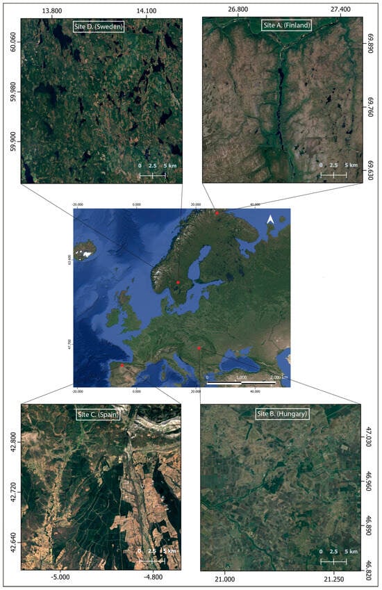
Figure 1.
Shows the location of the four study sites across Europe.
Site A: The northern tip of Finland is a part of the Scandinavian Montane Birch Forests and Grasslands ecoregion. The Utsjoki valley is covered in expanses of montane birch forests above the coniferous zone; high precipitation during the growing season enables abundant growth of some vascular plants and mosses [37]. The region beyond the conifer tree line is dominated by Birch (Betula nana L.), Willow (Salix alba L.), flowering plants (Empetrum nigrum L., Rubus chamaemorus L.), lichens (Cladonia deformis (L.) Hoffm., Cladonia chlorophaea (Flörke) Fr.), and mosses (Sphagnum fuscum (Schimp.) H. Klinggr.) [38]. This forest region has been historically managed for timber production; the thinning of forests makes it less resilient to local disturbances, thus increasing its vulnerability to climate change [39]. Conditions in Northern Lapland are ideal for the formation of palsa mires with low precipitation (<450 mm) and a mean annual air temperature of −3 °C to −5 °C [40]. This region will provide insight into the climatic sensitivity of the ecotone between the tundra and taiga biomes, peat bogs, and managed forests in northern Finland, the dynamics of which are anticipated to change due to climate change.
Site B: Southeast Hungary, part of the Pannonian Mixed Forest ecoregion, has a mean annual temperature range of 10–11 °C and the annual rainfall averages at >650 mm [41]. The local geomorphology, in conjunction with extreme temperatures and aridity in summers, gives rise to assorted landscapes categorized by enclosed oak forests, low and montane steppes (puszta), and floodplain vegetation [42]. The Sebes-Körös floodplain contains large arable plots with scattered patches of oak forests, riverine vegetation, and steppe grasslands, which became saline due to water regulation works in the 19th century [43]. Rare plant species of the saline landscape include Bassia sedoides (Pall.) Freitag & G.Kadereit, Camphorosma annua Pall., and Plantago schwarzenbergiana Schur, while the principal plant communities are Artemisio santonici-Festucetum pseudovinae and Agrostio stoloniferae-Alopecuretum pratensis. The region also has important loess species, including Phlomis tuberosa L. and Filipendula vulgaris Moench [43]. The two important vegetation zones in the area are the Bélmegyeri Fáspuszta and the Mágor Puszta, both of which are protected under the Körös-Maros National Park. The ecoregion is significant from a conservation standpoint because the typical open forest of the forest steppe with a mosaic-like structure is virtually unknown in other parts of Europe [44].
Site C. The southern slopes of the Cantabrian Mountain system in Leon, Spain, are a part of the Northwest Iberian Montane Forest ecoregion. The mean annual temperature ranges between −2.5 and 12.5 °C, and annual rainfall ranges from 700 to 1800 mm; the altitudinal gradient is 391–2650 m asl. [45]. Along the lowlands are croplands and meadows, while shrubs and heathlands cover the uplands. Herbaceous vegetation includes Cytisus multiflorus (L’Hér.) Sweet, Cytisus scoparius (L.) Link, Erica australis L., and Genista obtusiramea J. Gay ex Spach, etc. [46]. The Atlantic vegetation of the region consists of deciduous forests with Fagus sylvatica L., Betula pubescens Ehrh., Quercus petraea (Matt.) Liebl., and Q. robur L. The region is also part of the Guardo-Barruelo coal basin, with a history of open-cast mining, and reclamation efforts are now underway at some of these mines [47]. However, decades of mining activities have had a severe impact on local herbaceous diversity and patterns of biomass accumulation [47]. The site will help in the comprehension of land cover dynamics in the Mediterranean–Oceanic transition zone and along elevation gradients of the Southern Cantabrian Mountains.
Site D. This site lies in the southern boreal zone of Sweden, a part of the Scandinavian and Russian taiga ecoregion. The region has a mean air temperature of 5.2 °C and a mean annual precipitation of 854 mm [48]. The southern boreal forest subzone is dominated by forests of Pinus sylvestris L., Picea abies (L.) Karst., Alnus incana (L.) Moench and Betula nana L. are also common [49]. The region contains scattered water bodies and peat bogs. The peat bog vegetation is dominated by Sphagnum spp., with sparse occurrences of Eriophorum vaginatum L., Calluna vulgaris (L.) Hull, Andromeda polifolia L., and Rubus chamaemorus L. [50]. The silviculture practices in south-central Sweden have favored conifers for decades, and the accompanying decrease in broadleaf vegetation has been termed “borealization” [51]. Consequently, the naturalness of the south-central Swedish boreal remains low despite its extensive forest cover [52]. As the largest ecoregion in Europe, it is crucial to comprehend the landscape dynamics of boreal forests in light of climate change. This site will provide an understanding of the land cover dynamics in the boreal-hemiboreal ecotone.
2.3. Preparation of Habitat Maps
Habitat maps from 2000 and 2018 for the four sites were compared at the class level to determine the change in classes. A supervised classification with a maximum likelihood parametric rule was performed using ERDAS Imagine software version 16.7.2 to create habitat maps. Landsat 7 and Landsat 8 (USGS) data for the years 2000 and 2018, respectively, were used as input data. Supplementary Information Table S1 provides a list of satellite data and regional reference data used for the preparation of LULC maps. The uniformity across four locations was maintained by adhering to CORINE classification requirements and CORINE Land Cover (CLC) Level 3 class descriptions. The classes of the CLC nomenclature are a mixture of land cover and land use information pertinent to the actual landscape features of Europe [16], making the CLC a suitable choice for this study. It is important to note that LULC classes map homogenous landscape patterns into discrete classes and do not represent the spatial distribution of biodiversity; however, the Corine classes can be interpreted to identify major EUNIS habitat types [53] and their description can be obtained from EEA website (https://eunis.eea.europa.eu/habitats-names.jsp; accessed on 18 October 2025) (See Supplementary Data Table S2. For the CLC classes used and the habitat type they signify). Where available, regional high-resolution land cover maps (20–25 m) were resampled to 30 m resolution to match Landsat data and were used to cross-validate the findings of a supervised classification. Accuracy assessment of habitat maps can be found in Table S3 (A–D) in the Supplementary Information. The overall classification accuracy was 86%. Unsurprisingly, the highest accuracy was obtained in Site A (Finland), where the reference map was from the same year and of comparable resolution (kappa = 0.94). Kappa coefficient values in all other sites ranged from 0.81 to 0.84, where reference maps were either not from the same year, had a different classification system (Site D, Sweden), or both (Sites B and C in Hungary and Spain, respectively). The lowest accuracy was obtained in the classification of coniferous forest at the Spanish site (71%) and pasture category at the Hungarian site (74%).
2.4. Ecosystem Functions and Pressures
Water Yield (WY) and Aboveground Biomass (AGB) are the ecosystem functions used for this study. This choice was based on the ability of these measures to provide information about key regulating and provisioning ecosystem functions affected directly by land use change [54]. Additionally, due to their widespread use, the availability of standardized datasets and literature-based coefficients allowed a consistent comparison across diverse sites where local empirical data are lacking. As the empirical calculation of ecosystem functions is outside the scope of this study, proxy values and existing data were utilized to approximate the per-hectare values of WY and AGB in different habitat classes.
Water Yield: Changes in habitat type can impact hydrologic cycles, altering patterns of evapotranspiration, infiltration, and water retention, as well as the timing and quantity of available water (InVEST User Guide, 2020). Here, WY was estimated using the coefficients of runoff [55] and precipitation data. The following Equation (1) was used:
where A = area of LULC class in ha, P = precipitation in mm, and YC = coefficient of runoff.
Since precipitation data at an appropriate resolution for both 2000 and 2018 across Europe were not available from a single source, precipitation data for the year 2000 were downloaded from Worldclim.org in the form of the average monthly precipitation data at 30″ resolution. For 2018, Data Repository for Atmospheric Science and Earth Observation’s Climatic Research Unit (CRU) Time-Series (TS) version 4.04 precipitation data at 10″ resolution was used and was resampled to match the resolution of precipitation data from 2000. These data were processed in QGIS 3.8.2 for annual average precipitation. Average annual precipitation data were then extracted for each land cover class using the “Zonal statistics” tool. Coefficients of runoff for CORINE land cover classes were taken from Cecchi et al. (2007) [56]. See Supplementary Information Table S4 for the values used.
Aboveground Biomass: AGB is a key component of the global carbon cycle and plays an important role in climate change through carbon sequestration and storage. Previous studies show that remote sensing can efficiently quantify and monitor regional forest biomass [57]. The ESA CCI Carbon Map [58] was used to estimate average AGB (Mg/ha) in each class using the ‘zonal statistics’ tool in QGIS. These baseline values were used to estimate change due to the transition of classes (Supplementary Information Table S4).
In QGIS, an ‘intersection’ was performed on the 2000 and 2018 maps to ascertain the area remaining in the same class in both years; classes of the remaining area were used to determine the transitions occurring and create a transition matrix. Based on the available literature on local contexts, the pressures behind each change event were identified. The total area of individual sites under different pressures was determined by summing the areas of transitioning classes associated with a given pressure.
Pearson’s coefficient of correlation is a statistical measure that defines the relationship between two variables. This relationship is characterized by values between −1 and 1 and can be negative or positive. The further away from zero the values are, the stronger the positive or negative association becomes [59]. R values were used to find a correlation between the area covered by various pressures and the change in AGB and WY.
3. Results
3.1. Habitat Dynamics
Out of the 160,000 ha across four sites examined in this study, 33,516.62 ha (or 20.94% of the total area) underwent a change in habitat class. Changes were not uniform across similar habitat types. Amongst herbaceous vegetation, we see a reduction in the original range of natural grasslands (−36%) and sclerophyllous vegetation (−40%), whereas heathlands and moors in the north show a significant expansion (59%) (Figure 2). Similarly, in forest habitats, coniferous forests decreased by 15.7% in 2018, while broadleaf and mixed forests continued to expand (by 17.3% and 27.8%, respectively). The biggest loss was seen in the transitional woodlands/scrubs, which lost 8878 ha across the four sites by 2018. Some of this loss was offset by a gain of 2142.02 ha in agricultural areas and 1320.29 ha in open areas with little or no vegetation. Net change in other classes was less than 500 hectares of land area.
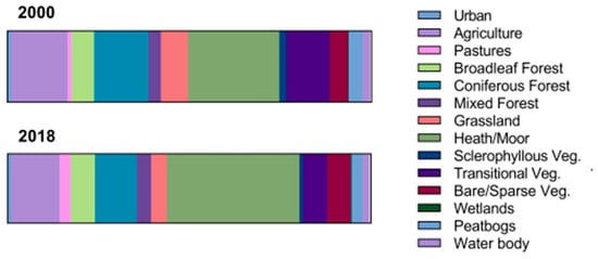
Figure 2.
Change in the proportion of different habitat classes between the years 2000 and 2018 based on habitat maps derived from satellite imagery using CLC classification.
Figure 3 shows a Sankey diagram for the top ten habitat transition events across each site. The full 2000–2018 transition matrices are provided in the Supplementary Information (Table S5(a–d)). In site A (Finland), the highest magnitude of change was observed in transitional woodlands/scrub habitats with 9247.2 ha transitioning into heathlands and 1358.3 ha into wetland habitats by the year 2018. Other significant changes ranged between 1000 and 2000 ha and involved the transition of broadleaf forests into heathlands and heathlands into open areas with little or no vegetation. Most changes (87%), however, involved an area of <500 ha; 77% and 76% of changes involved areas under 100 ha and 50 ha, respectively. In site B from Hungary, the most notable changes were associated with habitat classes of agricultural type (croplands and pastures) and grassland. 1531.8 ha and 1688.2 ha of croplands transitioned into habitat classes of pastures and broadleaf forests by 2018, respectively. A combined area of 2970 ha of grasslands was transformed into agricultural classes of croplands and pastures between 2000 and 2018. Only 15% of all changes involved habitat changes of >500 ha, and 10% involved area >1000 ha.
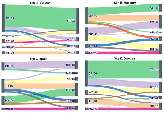
Figure 3.
The Sankey diagram shows the top ten habitat transition events across each site between 2000 and 2018. Year code: _00: 2000; _18: 2018. Habitat code—AR: Artificial; CR: Croplands; PS: Pastures; BR: Broadleaf; CF: Coniferous; MX: Mixed Forest; GR: Grassland; HT: Heathlands; SC: Sclerophyllous scrub; TR: Transitional; OA: Open areas with little/no vegetation; WT: Wetland; AQ: Aquatic (Inland).
In Site C (Spain), the most significant changes involved the transition of mixed forests and transitional woodlands into coniferous forests and the transition of grasslands into pastures between 2000 and 2018. These were the only changes that involved areas covering > 1000 ha. Similarly to Site A in Finland, 86% of change events involved an area of less than 500 ha, 59% of the total changes were under 100 ha, and 50% were under 50 ha. At site D (Sweden), the most heavily transformed habitat class was coniferous forests, with 7476.4 ha transitioning into transitional woodlands and 2624.9 ha into mixed forests by 2018. Other notable changes (ranging 1000–2000 ha in magnitude) included transitional woodlands changing to coniferous forests and wetland habitats being replaced by mixed forests in 2018. As seen in Sites A and C, most habitat changes in Site D (73%) also involved change events of < 100 ha, with only 6% changes including an area > 1000 ha.
Figure 4 (below) shows the frequency of different change events across the four sites. The groups with the largest area in 2000, semi-natural areas and forests, recorded the largest number of class transitions. Despite a slight change in overall area, 10,432.29 ha of forest habitat underwent changes between 2000 and 2018, indicating a significant rate of intra-class transitions. The inter-class transition between herbaceous and woodland habitats constituted the majority of all transitions, whereas artificial habitats and freshwater aquatic habitats experienced no significant change. Based on data across all four sites, the distribution of change-event sizes was highly skewed: 99% of events were small-scale (0–3082 ha), 0% intermediate (3082–6164 ha), and only 1% large-scale (6164–9248 ha). Just two large-scale events were recorded, both occurring in the northern sites A (Finland) and D (Sweden). When applying an ecologically meaningful distinction between local (<100 ha) and landscape (>100 ha) changes [60], 72% of events were local, 22% meso-landscape scale (100–1000 ha), and 6% were macro-landscape scale (>1000 ha).
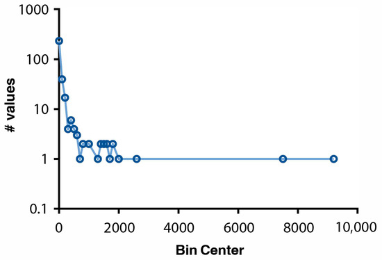
Figure 4.
Log-linear figure showing the frequency of change events across the four sites. The y-axis shows the log10 of the number of values, and the x-axis shows the bin size of the area in hectares.
3.2. Identifying Pressures
The investigation of the transition matrix, the patterns observed in nature, and the direction of land cover type changes led to the identification of seven major pressures acting on landscapes. In lieu of conventional definitions, these pressures are specified here in reference to the local scale at which they are being investigated.
The BIOPRESS project initially identified six major pressures on biodiversity—urbanization, intensification, afforestation, deforestation, abandonment, and drainage. Later studies have included other pressures, such as rewetting, afforestation, and extensive urbanization, which are still relevant issues worldwide, among others, to better explain regional habitat changes [23]. Since the nature of pressures has changed since the original study (conducted in the early 2000s), the interpretation of some of the transitions had to be changed based on local context. Across the four sites studied, the level of urbanization was low, and the rate of intensification has also considerably reduced; hence, urbanization and intensification have been combined into one category, ‘Conversion’. It also includes the conversion of “wet” classes into artificial (urban and agricultural) habitat classes. Categories of afforestation and abandonment have also been replaced by a single category of ‘Regrowth’ that can describe regrowth of vegetation after natural or anthropogenic stressors (e.g., abandonment (regrowth of non-woody vegetation) and afforestation (regrowth of woody vegetation)) across different habitat types. Degradation is another category introduced to explain the natural degradation of vegetation not addressed by other categories. It also includes degradation of “wet” classes as a result of drainage due to natural causes. Due to the low levels of human-induced drainage observed, drainage conducted for agricultural or urbanization purposes is included in ‘Conversion’, as mentioned earlier. A category ‘Encroachment’ is added to address the advancement of woody vegetation into wetlands and inland water bodies, a problem increasingly reported in European wetlands [61,62,63], but not addressed by other categories. The pressure ‘Wetting’ is used instead of ‘rewetting’ to categorize the transition of ‘dry’ classes into wetlands/water bodies, since re-wetting implies the habitat class was a wetland/inland water body class at some point, which is not always the case [23,64]. Category of ‘Range shift’ has been added to address the inter- and intra-class transitions of semi-natural and natural habitat classes which are traditionally not considered a pressure on biodiversity due to no net loss in the habitat size; however, studies show that changes in configuration can have several impacts of local biodiversity in form of edge effects, dispersal declines, etc. [28,65,66,67]. Furthermore, the changing ranges of habitat classes associated with changing temperature and rainfall patterns can have severe long-term impacts on biodiversity (such as a reduction in population sizes or extinctions at the range edges) [68,69,70]. Table S6 (Supplementary Information) provides a side-by-side comparison of previously used pressure categories under the BIOPRESS methodology and those used in this study. Figure 5. shows how different class transitions were linked to the pressure categories mentioned above. The definitions of various pressures identified in this study are listed below; in lieu of conventional definitions, these pressures are specified here in reference to the scale at which they are being investigated:
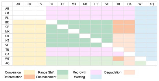
Figure 5.
Illustration showing the categorization of different pressures identified based on class transitions across the four sites. Habitat code—AR: Artificial; CR: Croplands; PS: Pastures; BR: Broadleaf; CF: Coniferous; MX: Mixed Forest; GR: Grassland; HT: Heathlands; SC: Sclerophyllous scrub; TR: Transitional; OA: Open areas with little/no vegetation; WT: Wetland; AQ: Aquatic (Inland).
- Conversion (CV): the use of natural or semi-natural areas for anthropogenic activities such as agriculture, building commercial units, industries, etc.
- Deforestation (DF): cutting of forests for timber production or the extraction of other forest products.
- Degradation (DE): the degeneration of vegetation via a decrease in species richness, diversity, and/or biomass.
- Encroachment (EN): the advancement of woody vegetation into inland marshes, inland water bodies, and peat bogs.
- Wetting (WT): the conversion of natural/ semi-natural classes into wetlands and/or water bodies.
- Range shift (RS): the spatiotemporal change in distribution limits of habitat types along altitudinal or latitudinal gradients. This pressure excludes changes in and around inland aquatic habitat (wetting, encroachment) and any changes resulting directly from land conversion for human use (conversion).
- Regrowth (RG): the growth of vegetation on formerly bare land or abandoned agricultural land, regrowth of vegetation after natural or anthropogenic stressors (fire, clearcutting, etc.), natural change (or succession) in vegetation from non-woody to woody vegetation.
Regrowth accounted for 36.88% of the total transitioned area of 57,998.55 ha, followed by Range Shift (20.62%) and Deforestation (15.62%). The area impacted by Encroachment and Wetting was the smallest of the seven pressures identified. Four sites in four distinct ecoregions were impacted by different combinations of stressors. Site A has the largest area affected by pressures, with 19,861.39 hectares, followed by Site B with 18,854.48 hectares (Table 1). The occurrence of different pressures at various sites is detailed below.

Table 1.
Area under different pressures in individual sites.
3.3. Habitat Types and Associated Pressures
Regrowth: Regrowth, which was mostly observed in classes affected by silviculture and land abandonment, was the biggest pressure by area, affecting 10.11% of the total study area (160,000 ha) (as seen in Figure 6 below). The main transition resulting from Regrowth was observed in the class of transitional woodlands/scrub, which changed to natural and semi-natural vegetation classes in 2018. Regrowth of forests and non-woody vegetation occurred in 5985.62 ha and 9247.24 ha of transitional woodlands/ scrub, respectively. 25.29% of Site A was affected by Regrowth, the highest area covered by any pressure across all sites.
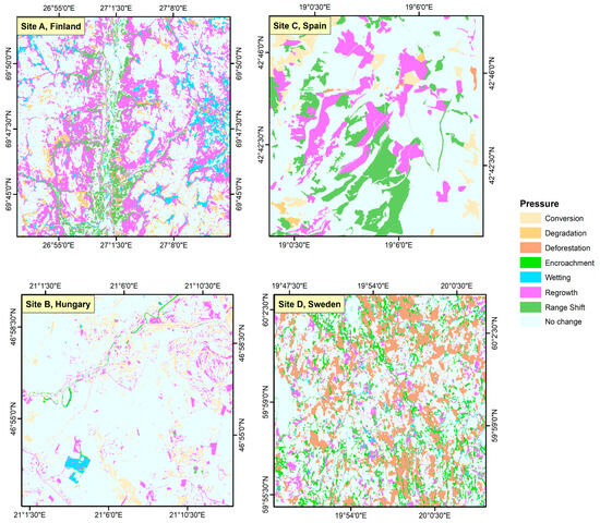
Figure 6.
Shows the distribution and extent of different pressures behind biodiversity loss associated with each site.
Range Shift: The occurrence of this phenomenon was seen to increase with altitude (Site C) and latitude (Site A). The area affected by Range Shift was largest in Site C, which has the highest forest cover of all sites, and the habitat types most affected. Range Shift, although leading to a lesser number of transitions, affected a larger area in Site C as compared with Site A, despite being at a lower elevation and latitude.
Interchange of ranges: Between 2000 and 2018, 958.58 ha of coniferous forests and 1147.73 ha of mixed forests were replaced by broadleaf forests in three of the four sites, while the reverse only took place in 665.81 ha of broadleaf forests. In site C, coniferous and broadleaf forests replaced 50% of the mixed forest in the region. In Site D, most range shifts occurred along the boundaries of forest patches, where broadleaf and mixed vegetation replaced 14.4% of the coniferous forests in the area. In turn, these areas were replaced by 200 and 724 ha of coniferous forests, respectively.
Range expansion and contraction: In Site A of the Scandinavian Montane Ecoregion, 1268.55 ha of previously forested land were occupied by the habitat class of heathlands and moors in 2018; this expansion mostly occurred within the elevation range of 227 ± 48 m, nearing the upper elevation limit of forests in the region. In the Cantabrian Mixed Forest of Spain, the elevation range of sclerophyllous vegetation was reduced by 90 m, and the mean elevation increased by 23 m above sea level (asl) to 1095 m asl, indicating habitat contraction at lower elevation limits, which was replaced by grasslands (Figure 6).
Deforestation: Deforestation affected 5.38% of the total study area and was more prevalent in coniferous forests of Site D, where 7476.34 ha or 8.21% of coniferous forests changed to transitional woodlands between 2000 and 2018. Deforestation in other sites was less severe, affecting a combined area of 605.11 ha in the remaining three sites.
Conversion: Northern sites A and D were less affected by this pressure than southern and central European sites. In site B, 2951.85 hectares of grasslands were converted to cropland and pasture. Site C in Spain also showed a similar trend of increasing conversion of grasslands for agricultural use, particularly along the southern slopes of the Cantabrian Mountain range.
Degradation: Degradation was only observed in sites A and C. The main transitions resulting from degradation were a change in herbaceous vegetation to bare areas, as observed at Site A. In site C, the eventual change in transitional woodland/scrub into grasslands was also categorized as degradation.
Wetting: The main transitions seen as a result of Wetting included conversion of peripheral woody or herbaceous vegetation around peat bogs into peat bog vegetation (Sphagnum spp., Eriophorum vaginatum L., etc.) or ponds. Most notably, this conversion is seen at Site A, where 2286.392 ha of transitional woodlands and broadleaf vegetation around peat bogs was classified as peat bogs in 2018 (Figure 6). A similar conversion is observed in Site D, albeit to a considerably lesser extent. In site B, the Wetting was mostly observed in small pockets across agricultural classes of cropland and pastures.
Encroachment: This pressure was most prevalent in peat bogs of Swedish site D, which saw increased encroachment of mixed forests into peat bogs, leading to a 44.93% contraction in the original area covered by peat bogs in 2000. Encroachment observed in site A was mostly by herbaceous and transitional vegetation and only affected 426.68 ha of peat bogs. No significant encroachment of aquatic habitats was seen in Site B and Site C.
3.4. Ecosystem Functions
Water Yield: As a result of land cover transitions between 2000 and 2018, there was a combined decrease of 246 ML in Water Yield in the four sites (Table 2). Regrowth (RE) had the highest (negative) effect on Water Yield. Pressures associated with loss of forest cover—Conversion, Deforestation, and Degradation—led to an increase in Water Yield. Conversion of ‘dry’ land cover classes to ‘wet’ classes under the pressure of Wetting had a negative effect on Water Yield. The effects of Range Shift and Encroachment were minimal (−19.16 and +8.99 ML, respectively). Out of the four sites, an increase in Water Yield was only observed in Site A, and Site B was the least affected by changing Water Yield. Significantly higher negative effects on Water Yield were seen for Site C and Site D. Range Shift had an opposite effect in Site A, where it caused an increase in Water Yield. Similarly, Encroachment in site D caused a decrease of 0.19 ML in Water Yield, as opposed to its positive effect on other sites.
Table 2.
Increase/Decrease in AGB and WY due to various pressures between 2000 and 2018.
Aboveground Biomass: Across the four sites, land cover change resulted in a total decrease of 91.68 Mg/ha in average aboveground biomass density. The most significant change was caused by Wetting, which was associated with a decrease of 93.15 Mg/ha, followed by Deforestation (−69.46 Mg/ha) and Conversion (−34.99 Mg/ha) (Table 2). Encroachment, which caused transition of classes in a direction opposite to Wetting (i.e., from wetlands to ‘dry’ vegetation class), had the highest positive effect on aboveground biomass. Regrowth was the only other pressure that resulted in an increase in aboveground biomass (by 50.89 Mg/ha). Out of the four sites, average aboveground biomass was only seen to increase in Site B, specifically as a result of Regrowth and Encroachment. Wetting and Deforestation were the leading causes of the average aboveground biomass decline of 66.61 Mg/ha in Site C. Decrease in aboveground biomass because of Regrowth in Site A and its increase as a result of Regrowth in Site C were the two unusual trends in the direction of aboveground biomass change.
All the pressures had an opposite effect on AGB and WY (Figure 7). Overall, WY was more strongly affected by various pressures behind land cover transitions than AGB. Conversion (0.94) and Deforestation (0.99) had a strong positive relationship with WY, while Wetting had a strong negative influence (−0.99); all three had a weak correlation with AGB. Degradation and Regrowth had a moderately favorable impact on WY and a moderately negative impact on AGB. The correlation of Regrowth and Encroachment to AGB (−0.61 and 0.69, respectively) was the only moderately strong relationship of AGB to any pressure. Range shift had a weak correlation with both AGB and WY.
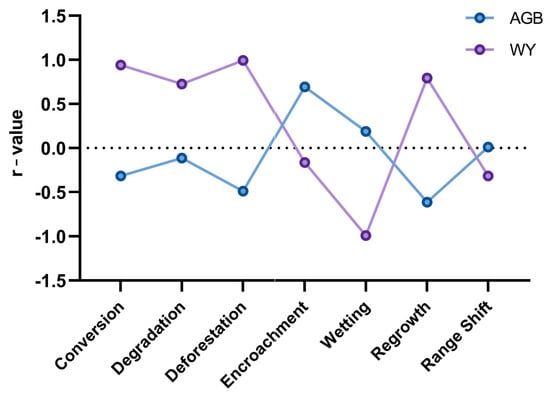
Figure 7.
Pearson’s r-value for change in AGB and WY with respect to different pressures.
4. Discussion
This study provides an overview of the relationship between various pressures that lead to habitat changes across coldspot sites from four different ecoregions in Europe and associated changes in the ecosystem functions of Aboveground Biomass and Water Yield. By including diverse habitats and applying BIOPRESS methodology at a smaller scale, the study is able to highlight conservation needs across a spectrum of habitat types and introduce new pressure categories present in biodiversity coldspots of Europe. The results show scrub and/or herbaceous vegetation experiencing a high rate of transition under pressures such as Range expansion/contraction, Degradation, and Conversion. Despite a decline in other agricultural categories, pastures at Sites B (Hungary) and C (Spain) have continued to expand. The conversion of grasslands to pastures on the lower slopes in NE Spain might be a result of a decrease in ‘transmittance grazing’ (i.e., movement of cattle to uplands during summer months) due to agricultural intensification and change from sheep grazing to cattle grazing [18]. Increasing conversion of grassland to pasture in the Sebes-Körös plain of Hungary can also be attributed to changes in management practices. Around 19% of grasslands in Hungary are affected by unfavorable grazing and mowing [71]. There is also evidence of range contraction in the Hungarian dry-steppe and mesophilous-steppe grasslands in response to changing grazing patterns resulting from agricultural abandonment [72].
In addition to the loss of natural grasslands, we also observe a decline in sclerophyllous vegetation, which is mostly attributed to Range Shifts. A combination of climate change and land cover changes is known to propel upslope movement of vegetation [73]. The results correspond with previous findings reporting increasing range contraction in Mediterranean mountain vegetation [74,75], particularly in sclerophyllous vegetation. Transitional vegetation, which represents zones of regeneration after clear-cutting or natural disturbance, showed mixed patterns in the three sites where it was present. In Site A, most of the transitional woodlands changed into either broadleaf forests or heathlands; this can be attributed to the successful or failed regeneration in logged areas, respectively. In site C, we see regeneration of coniferous vegetation in a previously fire-damaged zone classified under transitional vegetation. The only herbaceous vegetation class to have expanded was the sub-arctic heathlands of Northern Finland. Various studies have predicted expansion of the sub-arctic heath community because of a change (increase) in temperature and subsequent increased nutrient availability resulting from enhanced litter decomposition rates [76,77].
In addition to the deforestation-regrowth cycle in forested classes, a lot of habitat change was brought about by the Range Shift. While range shifts can have positive outcomes, such as increased colonization potential and expansion into new territories, they are also accompanied by risks; Climate change—driven shifts may reduce populations of species unable to track suitable climates, and significant losses can occur at contracting edges where specialized or less mobile assemblages are displaced [69,78]. Secondary literature can provide ecological and management context to understand the drivers and effects of range shift in coldspots. Despite a preference for conifer monocultures in managed Swedish Boreal forests [76], results for Site D indicate coniferous forests are replaced by broadleaf and mixed forests. An increase in Birch has been reported throughout Sweden in the last decade [79] and can be attributed to the changes in environmental policies and certification schemes that are now promoting mixed regeneration [80]. Scandinavian birch forests of Site A, however, showed a decline. Although a warming climate is expected to facilitate the expansion of Birch forests in Northern Finland, the increased frequency of pest outbreaks [39] and pressure from reindeer grazing has been reported to affect the broadleaf vegetation of the area [81].
The results show significant Encroachment of woody vegetation in peat bogs and inland marshes of Site D in Sweden. Climate change is suspected to be facilitating woody encroachment in Sphagnum-dominated bogs; Warmer climates are conducive to the establishment of cold-suppressed tree seedlings [82], and atmospheric nitrogen deposition leads to increased nitrogen availability to vascular plants in these nitrogen-deficient ecosystems [83]. In Site A, the area classified as peat bogs increased in 2018 under the pressure described here as Wetting; peat bogs were seen to expand into transitional woodlands. There are two possible explanations for this: 1. Loss of transitional woodlands surrounding the peat bogs may be caused by changing climatic conditions, which support the expansion of vegetation such as graminoids, which are better supported by wetter sites [84] 2. The formation of “Thermokarsts” or small ponds formed on the melting of Palsa mires/bogs [85] can explain the expansion of inland water bodies observed from satellite images.
We observed no land transitions at the intermediate bracket of the data distribution (i.e., involving areas between 3000 and 6000 ha), and most habitat transitions occur on a small scale, with a few large-scale transitions concentrated in sites with active silvicultural practices. A comparable pattern has been reported in the UK, where at the national level, there was a clear gap in the distribution of habitat change events, and the ones associated with forest habitats involved a disproportionately larger area [23]. At biogeographical scales, older analyses across Europe (changes between 1990 and 2000) also showed the majority of changes occurring through smaller transition events, but showed a varying pattern of distribution of change for intermediate and large-scale events [14]. Thus, the observed lack of intermediate-scale events could be scale-dependent.
The observed decrease in water yield (WY) in areas undergoing Wetting (Figure 7) is a notable discrepancy that requires further explanation. In this study, Wetting refers to the conversion of dry habitats into wetlands or water bodies, which act as endpoints for runoff and were therefore assigned a low runoff coefficient (0.1) in the WY calculation. Consequently, Wetting showed a negative correlation with WY, reducing it by 50 ML across the four sites. This outcome reflects a methodological limitation, suggesting that complementary indicators such as changes in water storage or overall water availability are needed to capture the full hydrological implications of Wetting as a pressure. It is also important to note that the calculation of Water Yield includes the run-off coefficient for each land cover class, whereas AGB was extracted from a dataset with a lower resolution than that of the input habitat maps. This makes Water Yield significantly more sensitive to changes in class type, resulting in a stronger correlation with the pressures. The unexpected effects of Range shift and Regrowth effects on WY can also be explained by some high AGB classes, like forests, having low per-pixel annual precipitation values.
This study has shown how in the European biodiversity coldspots, habitat transitions can be shaped by numerous small-scale disturbances from local pressures, compounded by climate change and adverse management, with direct consequences for ecosystem functioning. Results show habitat change occurring in 20% of the area across the four test sites; however, at the European scale, these areas have previously been classified under stable zones (e.g., [3]). This helps us reemphasize that conservation planning must extend beyond large, species-rich hotspots [8] to also include fragmented and transitional habitats where subtle changes accumulate into significant functional losses. In practice, this means valuing hotspots for their rich biodiversity while systematically integrating coldspots to secure ecosystem services, buffer climate impacts, and maintain ecological connectivity.
Policy instruments can support this integration. EU Nature Restoration Targets [86] could include corridor and buffer zones across elevational and climatic gradients to accommodate the range shifts in the sub-arctic heath and Mediterranean montane shrubs community. Within the EU’s goal of protecting 30% of land [87], allocating even ~5% to coldspots, especially in temperate grasslands and transitional areas, would ensure the protected area network becomes more responsive to its role in complementing hotspots under accelerating land use and climate pressures. Where continuous conservation zones are not feasible, micro-reserves nested within a broader protected area network (e.g., Natura 2000 [88]) could safeguard small but functional units (e.g., patches of endemic grasslands, peat bogs storing carbon, or transitional zones enabling natural regeneration), even if species richness is low.
Limitations and Future Directions
The interpretation of habitat dynamics at a local scale for geographically and ecologically diverse regions is challenging and leads to certain limitations. Firstly, maintaining consistency of datasets for the four different sites at two time periods is challenging. For instance, no reference data was available for land cover classification of Site B in the year 2000, and only Landsat 7 data was used. This can lead to errors in demarcation and identification of classes of similar appearance, such as pastures and grasslands, which showed a lower classification accuracy (74–79%) (Supplementary Information Table S3). Consequently, some transitions may have been misclassified as regrowth or conversion, and in these habitats, identified pressures should be interpreted cautiously. Secondly, the complex nature of evaluating ecosystem functions also leads to certain limitations, and the proxy measures used here only provide indicative trends rather than precise estimates. The simplified equation used for the calculation of WY does not account for the effects of topography, soil heterogeneity, evapotranspiration, or land management practices, all of which can substantially influence water yield. Additionally, the standard coefficients of runoff were assigned uniformly across habitat classes in all four sites, but two of the same classes at different locations can have different coefficients of runoff [89]. This makes WY results sensitive to coefficient assumptions and highlights the need for caution in interpretation. In the future, a process-based model (e.g., InVEST, SWAT, etc.) that is able to capture these dynamics can be considered [90]. Lastly, EO-derived AGB estimates are only indirectly related to biomass and run on various assumptions; cross-validation of ESA CCI AGB (2018) data with field inventory data showed a bias of 2.3 Mg/ha [91]. The spatial resolution of this data is also coarser than the Landsat-based habitat maps used in this study. This mismatch may smooth out local-scale biomass variation and introduce biases in heterogeneous landscapes. Future studies can employ Machine Learning methods to match the resolution of ESA CCI AGB maps to input satellite data, where in situ data is available [92]. Overall, improvements such as field validation campaigns, integration with climate projections, and coupling with species distribution models would strengthen future analyses and enable more mechanistic assessments of biodiversity outcomes.
5. Conclusions
In conclusion, this study shows how even with a limited increase in human activity and direct damage to habitat classes in biodiversity coldspots, climate change is playing a strong role in driving changes in the composition and structure of vegetation. Several key trends identified here can inform the strategic expansion of Protected Area networks. Firstly, despite no overall loss of forests, there is a notable decline in above-ground biomass per hectare and an increase in water yield, indicating heightened runoff rates, largely driven by changes in herbaceous vegetation. Herbaceous species along ecotones at higher latitudes and altitudes are particularly vulnerable to local-scale habitat changes. Furthermore, inadequate management of grasslands in Southern and Central Europe poses a threat to endemic grassland species. Secondly, although substantial areas are undergoing regeneration, the majority of this activity occurs within managed forests rather than in natural habitats. This discrepancy reaffirms that not all reported regeneration contributes equally to biodiversity conservation. Thirdly, climate change poses threats beyond terrestrial vegetation, impacting wetlands and peat bogs with issues such as encroachment becoming more prevalent. Lastly, transitional zones between ecosystems will play an increasingly critical role in biodiversity conservation as climate change alters the boundaries of ecoregions. Effective management of these transitional areas requires consideration of the cumulative impacts of incremental habitat changes over the long term.
Supplementary Materials
The following supporting information can be downloaded at: https://www.mdpi.com/article/10.3390/su17209283/s1, Table S1: Description of satellite data and regional datasets used; Table S2: Description of EUNIS habitat types and corresponding CORINE Land Cover classes identified; Table S3: Accuracy assessment of supervised classification of habitat types; Table S4: Coefficient of runoff and Aboveground Biomass values used for each habitat type.; Table S5: Transitions matrix of habitat change across each site; Table S6: Comparison of previously defined pressure categories under BIOPRESS methodology with those used in this study.
Author Contributions
Conceptualization, A.K., H.B., and S.E.P.; methodology, A.K., H.B., and S.E.P.; software, A.K.; validation, A.K.; formal analysis and data curation, A.K.; writing—original draft preparation, A.K.; writing—review and editing, H.B. and S.E.P.; supervision, H.B. and S.E.P. All authors have read and agreed to the published version of the manuscript.
Funding
H. Balzter was supported by the UK Natural Environment Research Council as a member of the National Centre for Earth Observation.
Institutional Review Board Statement
Not applicable.
Informed Consent Statement
Not applicable.
Data Availability Statement
Data is contained within the article or Supplementary Material.
Conflicts of Interest
The authors declare no conflicts of interest.
References
- Reid, W.V.; Mooney, H.A.; Cropper, A.; Capistrano, D.; Carpenter, S.R.; Chopra, K.; Dasgupta, P.; Dietz, T.; Duraiappah, A.K.; Hassan, R. Ecosystems and Human Well-Being-Synthesis: A Report of the Millennium Ecosystem Assessment; Island Press: Washington, DC, USA, 2005. [Google Scholar]
- Foley, J.A.; DeFries, R.; Asner Gregory, P.; Barford, C.; Bonan, G.; Carpenter Stephen, R.; Chapin, F.S.; Coe Michael, T.; Daily Gretchen, C.; Gibbs Holly, K.; et al. Global Consequences of Land Use. Science 2005, 309, 570–574. [Google Scholar] [CrossRef]
- Kuemmerle, T.; Levers, C.; Erb, K.; Estel, S.; Jepsen, M.R.; Müller, D.; Plutzar, C.; Stürck, J.; Verkerk, P.J.; Verburg, P.H.; et al. Hotspots of land use change in Europe. Environ. Res. Lett. 2016, 11, 064020. [Google Scholar] [CrossRef]
- Gonzalez, A.; Cardinale, B.J.; Allington, G.R.H.; Byrnes, J.; Arthur Endsley, K.; Brown, D.G.; Hooper, D.U.; Isbell, F.; O’Connor, M.I.; Loreau, M. Estimating local biodiversity change: A critique of papers claiming no net loss of local diversity. Ecology 2016, 97, 1949–1960. [Google Scholar] [CrossRef] [PubMed]
- Jung, M.; Rowhani, P.; Scharlemann, J.P.W. Impacts of past abrupt land change on local biodiversity globally. Nat. Commun. 2019, 10, 5474. [Google Scholar] [CrossRef] [PubMed]
- Winkler, K.; Fuchs, R.; Rounsevell, M.; Herold, M. Global land use changes are four times greater than previously estimated. Nat. Commun. 2021, 12, 2501. [Google Scholar] [CrossRef]
- Kareiva, P.; Marvier, M. Conserving Biodiversity Coldspots Recent calls to direct conservation funding to the world’s biodiversity hotspots may be bad investment advice. Am. Sci. 2003, 91, 344–351. [Google Scholar] [CrossRef]
- Smithers, R.; Watts, K. Should we focus on biodiversity hotspots or biodiversity coldspots? In Proceedings of the Spatial Ecology & Conservation; University of Bristol: Bristol, UK, 2015. [Google Scholar]
- Dobrowski, S.Z.; Littlefield, C.E.; Lyons, D.S.; Hollenberg, C.; Carroll, C.; Parks, S.A.; Abatzoglou, J.T.; Hegewisch, K.; Gage, J. Protected-area targets could be undermined by climate change-driven shifts in ecoregions and biomes. Commun. Earth Environ. 2021, 2, 198. [Google Scholar] [CrossRef]
- Schrotter, M.; Kraemer, R.; CeauAyu, S.; Rusch, G.M. Incorporating threat in hotspots and coldspots of biodiversity and ecosystem services. Ambio 2017, 46, 756–768. [Google Scholar] [CrossRef] [PubMed]
- Bingham, H.; Lewis, E.; Belle, E.; Stewart, J.; Klimmek, H.; Wicander, S.; Bhola, N.; Bastin, L. Protected Planet Report 2020: Tracking Progress Towards Global Targets for Protected and Conserved Areas; Aston University: Birmingham, UK, 2021. [Google Scholar]
- Pimm, S.L.; Jenkins, C.N.; Li, B.V. How to protect half of Earth to ensure it protects sufficient biodiversity. Sci. Adv. 2018, 4, eaat2616. [Google Scholar] [CrossRef]
- Abeli, T.; Gentili, R.; Rossi, G.; Bedini, G.; Foggi, B. Can the IUCN criteria be effectively applied to peripheral isolated plant populations? Biodivers. Conserv. 2009, 18, 3877–3890. [Google Scholar] [CrossRef]
- Gerard, F.; Bugár, G.; Gregor, M.; Halada, L.; Hazue, G.; Huitu, H.; Kohler, R.; Kolar, J.; Luque, S.; Mucher, S.; et al. BIOPRESS: Linking pan-European land cover change to pressures on biodiversity. Available online: http://www.creaf.uab.es/biopress/index2.htm (accessed on 14 October 2025).
- Jaeger, J.; Soukup, T.; Schwick, C.; Madriñán, L.; Kienast, F. Chapter 20 Landscape Fragmentation in Europe: CORINE Land Cover Data; CRC Press: Boca Raton, FL, USA, 2016; pp. 157–198. [Google Scholar]
- Abdul Malak, D. Landscapes in Transition An Account of 25 Years of Land Cover Change in Europe; European Environment Agency: Copenhagen, Denmark, 2017. [Google Scholar]
- Luoto, M.; Pykälä, J.; Kuussaari, M. Decline of landscape-scale habitat and species diversity after the end of cattle grazing. J. Nat. Conserv. 2003, 11, 171–178. [Google Scholar] [CrossRef]
- Caballero, R.; Fernández-González, F.; Pérez-Badia, R.; Molle, G.; Roggero, P.P.; Bagella, S.; D’Ottavio, P.; Papanastasis, V.; Fotiadis, G.; Sidiropoulou, A.; et al. Grazing Systems and Biodiversity in Mediterranean Areas: Spain, Italy and Greece. Pastos 2009, 39, 9–154. [Google Scholar]
- Stoate, C.; Baldi, A.; Beja, P.; Boatman, N.D.; Herzon, I.; Van Doorn, A.; De Snoo, G.R.; Rakosy, L.; Ramwell, C. Ecological impacts of early 21st century agricultural change in Europe–a review. J. Environ. Manag. 2009, 91, 22–46. [Google Scholar] [CrossRef]
- Pach, M.; Sansone, D.; Ponette, Q.; Barreiro, S.; Mason, B.; Bravo-Oviedo, A.; Löf, M.; Bravo, F.; Pretzsch, H.; Lesiński, J. Silviculture of mixed forests: A European overview of current practices and challenges. Dyn. Silvic. Manag. Mix. For. 2018, 185–253. [Google Scholar] [CrossRef]
- Pohjanmies, T.; Triviño, M.; Le Tortorec, E.; Mazziotta, A.; Snäll, T.; Mönkkönen, M. Impacts of forestry on boreal forests: An ecosystem services perspective. Ambio 2017, 46, 743–755. [Google Scholar] [CrossRef] [PubMed]
- EEA. State of Nature in the EU: Results from Reporting Under the Nature Directives 2013–2018; European Environment Agency Publications Office: Copenhagen, Denmark, 2020. [Google Scholar]
- Cole, B.; Smith, G.; De La Barreda-Bautista, B.; Hamer, A.; Payne, M.; Codd, T.; Johnson, S.C.M.; Chan, L.Y.; Balzter, H. Dynamic Landscapes in the UK Driven by Pressures from Energy Production and Forestry—Results of the CORINE Land Cover Map 2018. Land 2022, 11, 192. [Google Scholar] [CrossRef]
- Smeets, E.; Weterings, R. Environmental Indicators: Typology and Overview; European Environment Agency Copenhagen: Copenhagen, Denmark, 1999; Volume 19. [Google Scholar]
- Connor, E.F.; McCoy, E.D. The statistics and biology of the species-area relationship. Am. Nat. 1979, 113, 791–833. [Google Scholar] [CrossRef]
- Hodgson, J.A.; Moilanen, A.; Wintle, B.A.; Thomas, C.D. Habitat area, quality and connectivity: Striking the balance for efficient conservation. J. Appl. Ecol. 2011, 48, 148–152. [Google Scholar] [CrossRef]
- McIntosh, A.R.; McHugh, P.A.; Plank, M.J.; Jellyman, P.G.; Warburton, H.J.; Greig, H.S. Capacity to support predators scales with habitat size. Sci. Adv. 2018, 4, eaap7523. [Google Scholar] [CrossRef] [PubMed]
- Pfeifer, M.; Lefebvre, V.; Peres, C.A.; Banks-Leite, C.; Wearn, O.R.; Marsh, C.J.; Butchart, S.H.M.; Arroyo-Rodríguez, V.; Barlow, J.; Cerezo, A.; et al. Creation of forest edges has a global impact on forest vertebrates. Nature 2017, 551, 187–191. [Google Scholar] [CrossRef]
- Fletcher, R.J.; Didham, R.K.; Banks-Leite, C.; Barlow, J.; Ewers, R.M.; Rosindell, J.; Holt, R.D.; Gonzalez, A.; Pardini, R.; Damschen, E.I.; et al. Is habitat fragmentation good for biodiversity? Biol. Conserv. 2018, 226, 9–15. [Google Scholar] [CrossRef]
- Jung, M.; Scharlemann, J.P.W.; Rowhani, P. Landscape-wide changes in land use and land cover correlate with, but rarely explain local biodiversity change. Landsc. Ecol. 2020, 35, 2255–2273. [Google Scholar] [CrossRef]
- Sharma, R.; Nehren, U.; Rahman, S.; Meyer, M.; Rimal, B.; Aria Seta, G.; Baral, H. Modeling Land Use and Land Cover Changes and Their Effects on Biodiversity in Central Kalimantan, Indonesia. Land 2018, 7, 57. [Google Scholar] [CrossRef]
- Burkhard, B.; Kroll, F.; Müller, F.; Windhorst, W. Landscapes’ capacities to provide ecosystem services—A concept for land-cover based assessments. Landsc. Online 2009, 15, 1–22. [Google Scholar] [CrossRef]
- Thomson, A.G.; Manchester, S.J.; Swetnam, R.D.; Smith, G.M.; Wadsworth, R.A.; Petit, S.; Gerard, F.F. The use of digital aerial photography and CORINE-derived methodology for monitoring recent and historic changes in land cover near UK Natura 2000 sites for the BIOPRESS project. Int. J. Remote Sens. 2007, 28, 5397–5426. [Google Scholar] [CrossRef]
- Hazeu, G.W.; Mücher, C.A. Historic Land Use Dynamics in and Around Natura2000 Sites as Indicators for Impact on Biodiversity; Phase 1 of the BIOPRESS Project for the Netherlands; Alterra: Wageningen, The Netherlands, 2005; pp. 1568–1874. [Google Scholar]
- Olson, D.M.; Dinerstein, E.; Wikramanayake, E.D.; Burgess, N.D.; Powell, G.V.N.; Underwood, E.C.; D’Amico, J.A.; Itoua, I.; Strand, H.E.; Morrison, J.C.; et al. Terrestrial Ecoregions of the World: A New Map of Life on Earth: A new global map of terrestrial ecoregions provides an innovative tool for conserving biodiversity. Bioscience 2001, 51, 933–938. [Google Scholar] [CrossRef]
- Bossard, M.; Feranec, J.; Otahel, J. CORINE Land Cover Technical Guide-Addendum 2000; European Environmental Agengy: Copenhagen, Denmark, 2000. [Google Scholar]
- Wehberg, J.; Thannheiser, D.; Meier, K. Vegetation of the Mountain Birch Forest in Northern Fennoscandia; Springer: Berlin/Heidelberg, Germany, 2005; p. 180. [Google Scholar] [CrossRef]
- Ruuhijärvi, R. The Finnish mire types and their regional distribution. In Mires: Swamp, Bog, Fen and Moor; Elsevier: Amsterdam, The Netherland, 1983; pp. 47–49. [Google Scholar]
- Venäläinen, A.; Lehtonen, I.; Laapas, M.; Ruosteenoja, K.; Tikkanen, O.-P.; Viiri, H.; Ikonen, V.-P.; Peltola, H. Climate change induces multiple risks to boreal forests and forestry in Finland: A literature review. Glob. Change Biol. 2020, 26, 4178–4196. [Google Scholar] [CrossRef]
- Luoto, M.; Heikkinen, R.K.; Carter, T.R. Loss of palsa mires in Europe and biological consequences. Environ. Conserv. 2004, 31, 30–37. [Google Scholar] [CrossRef]
- Nagy, G.; Nagy, L.; Kopecskó, K. Examination of the Physico-chemical Composition of Dispersive Soils. Period. Polytech. 2016, 60, 269–279. [Google Scholar] [CrossRef]
- Gábor, F.; Molnár, Z.; Magyari, E.; Somodi, I.; Zoltán, V. A new framework for understanding Pannonian vegetation patterns: Regularities, deviations and uniqueness. Community Ecol. 2014, 15, 12–26. [Google Scholar] [CrossRef]
- Molnár, Á.a.B.; Dániel; Széll; Antal; Biró; Marianna. Vegetation and vegetation changes of the Dévaványa-Ecsegi steppes in the last 15 years. In Crisicum; Periodical of The Körös—Maros National Park Directorate: Szarvas, Hungary, 2016; pp. 65–91. [Google Scholar]
- Fekete, G.; Király, G.; Molnár, Z. Delineation of the Pannonian vegetation region. Community Ecol. 2016, 17, 114–124. [Google Scholar] [CrossRef]
- Morán-Ordóñez, A.; Suárez-Seoane, S.; Elith, J.; Calvo, L.; De Luis, E. Satellite surface reflectance improves habitat distribution mapping: A case study on heath and shrub formations in the Cantabrian Mountains (NW Spain). Divers. Distrib. 2012, 18, 588–602. [Google Scholar] [CrossRef]
- García-Llamas, P.; Geijzendorffer, I.R.; García-Nieto, A.P.; Calvo, L.; Suárez-Seoane, S.; Cramer, W. Impact of land cover change on ecosystem service supply in mountain systems: A case study in the Cantabrian Mountains (NW of Spain). Reg. Environ. Change 2019, 19, 529–542. [Google Scholar] [CrossRef]
- Pallavicini, Y.; Alday, J.G.; Martínez-Ruiz, C. Factors Affecting Herbaceous Richness and Biomass Accumulation Patterns of Reclaimed Coal Mines. Land Degrad. Dev. 2015, 26, 211–217. [Google Scholar] [CrossRef]
- Jungqvist, G.; Oni, S.K.; Teutschbein, C.; Futter, M.N. Effect of Climate Change on Soil Temperature in Swedish Boreal Forests. PLoS ONE 2014, 9, e93957. [Google Scholar] [CrossRef]
- Giesecke, T. Holocene dynamics of the southern boreal forest in Sweden. Holocene 2005, 15, 858–872. [Google Scholar] [CrossRef]
- Borgmark, A.; Wastegård, S. Regional and local patterns of peat humification in three raised peat bogs in Värmland, south-central Sweden. GFF 2008, 130, 161–176. [Google Scholar] [CrossRef]
- Lindbladh, M.; Axelsson, A.-L.; Hultberg, T.; Brunet, J.; Felton, A. From broadleaves to spruce—the borealization of southern Sweden. Scand. J. For. Res. 2014, 29, 686–696. [Google Scholar] [CrossRef]
- Angelstam, P.; Manton, M.; Green, M.; Jonsson, B.-G.; Mikusiński, G.; Svensson, J.; Maria Sabatini, F. Sweden does not meet agreed national and international forest biodiversity targets: A call for adaptive landscape planning. Landsc. Urban Plan. 2020, 202, 103838. [Google Scholar] [CrossRef]
- Moss, D. EUNIS Habitat Classification–A Guide for Users; European Topic Centre on Biological Diversity: Paris, France, 2008. [Google Scholar]
- Zeng, L.; Liu, X.; Li, W.; Ou, J.; Cai, Y.; Chen, G.; Li, M.; Li, G.; Zhang, H.; Xu, X. Global simulation of fine resolution land use/cover change and estimation of aboveground biomass carbon under the shared socioeconomic pathways. J. Environ. Manag. 2022, 312, 114943. [Google Scholar] [CrossRef] [PubMed]
- Sriwongsitanon, N.; Taesombat, W. Effects of land cover on runoff coefficient. J. Hydrol. 2011, 410, 226–238. [Google Scholar] [CrossRef]
- Cecchi, G.; Munafò, M.; Baiocco, F.; Andreani, P.; Mancini, L. Estimating river pollution from diffuse sources in the Viterbo province using the potential non-point pollution index. Ann. Dell’Istituto Super. Di Sanità 2007, 43, 295–301. [Google Scholar]
- Li, Y.; Li, M.; Li, C.; Liu, Z. Forest aboveground biomass estimation using Landsat 8 and Sentinel-1A data with machine learning algorithms. Sci. Rep. 2020, 10, 9952. [Google Scholar] [CrossRef]
- Santoro, M.; Cartus, O. ESA Biomass Climate Change Initiative (Biomass_cci): Global Datasets of Forest Above-Ground Biomass for the Year 2017, v1. 2019; Centre for Environmental Data Analysis: Chilton, UK, 2019. [Google Scholar]
- Emerson, R.W. Causation and Pearson’s Correlation Coefficient. J. Vis. Impair. Blind. 2015, 109, 242–244. [Google Scholar] [CrossRef]
- Teng, S.N.; Svenning, J.-C.; Santana, J.; Reino, L.; Abades, S.; Xu, C. Linking Landscape Ecology and Macroecology by Scaling Biodiversity in Space and Time. Curr. Landsc. Ecol. Rep. 2020, 5, 25–34. [Google Scholar] [CrossRef]
- Pellerin, S.; Lavoie, M.; Talbot, J. Rapid broadleave encroachment in a temperate bog induces species richness increase and compositional turnover. Écoscience 2021, 28, 283–300. [Google Scholar] [CrossRef]
- Dieleman, C.M.; Branfireun, B.A.; McLaughlin, J.W.; Lindo, Z. Climate change drives a shift in peatland ecosystem plant community: Implications for ecosystem function and stability. Glob. Change Biol. 2015, 21, 388–395. [Google Scholar] [CrossRef]
- Butler, C.D.; Oluoch-Kosura, W. Linking future ecosystem services and future human well-being. Ecol. Soc. 2006, 11. [Google Scholar] [CrossRef]
- Magnússon, R.Í.; Limpens, J.; Kleijn, D.; van Huissteden, K.; Maximov, T.C.; Lobry, S.; Heijmans, M.M.P.D. Shrub decline and expansion of wetland vegetation revealed by very high resolution land cover change detection in the Siberian lowland tundra. Sci. Total Environ. 2021, 782, 146877. [Google Scholar] [CrossRef]
- Radford, J.Q.; Bennett, A.F. The relative importance of landscape properties for woodland birds in agricultural environments. J. Appl. Ecol. 2007, 44, 737–747. [Google Scholar] [CrossRef]
- Mimet, A.; Houet, T.; Julliard, R.; Simon, L. Assessing functional connectivity: A landscape approach for handling multiple ecological requirements. Methods Ecol. Evol. 2013, 4, 453–463. [Google Scholar] [CrossRef]
- Mimet, A.; Pellissier, V.; Houet, T.; Julliard, R.; Simon, L. A Holistic Landscape Description Reveals That Landscape Configuration Changes More over Time than Composition: Implications for Landscape Ecology Studies. PLoS ONE 2016, 11, e0150111. [Google Scholar] [CrossRef]
- Telwala, Y.; Brook, B.W.; Manish, K.; Pandit, M.K. Climate-induced elevational range shifts and increase in plant species richness in a Himalayan biodiversity epicentre. PLoS ONE 2013, 8, e57103. [Google Scholar] [CrossRef]
- Muluneh, M.G. Impact of climate change on biodiversity and food security: A global perspective—A review article. Agric. Food Secur. 2021, 10, 36. [Google Scholar] [CrossRef]
- Brooker, R.W.; Travis, J.M.J.; Clark, E.J.; Dytham, C. Modelling species’ range shifts in a changing climate: The impacts of biotic interactions, dispersal distance and the rate of climate change. J. Theor. Biol. 2007, 245, 59–65. [Google Scholar] [CrossRef]
- Molnár, Z.; János, B.; Horvath, F. Threatening factors encountered: Actual endangerment of the Hungarian (semi-)natural habitats. Acta Bot. Hung. 2008, 50, 199–217. [Google Scholar] [CrossRef]
- Somodi, I.; Virágh, K.; Aszalós, R. The effect of the abandonment of grazing on the mosaic of vegetation patches in a temperate grassland area in Hungary. Ecol. Complex. 2004, 1, 177–189. [Google Scholar] [CrossRef]
- Guo, F.; Lenoir, J.; Bonebrake, T.C. Land-use change interacts with climate to determine elevational species redistribution. Nat. Commun. 2018, 9, 1315. [Google Scholar] [CrossRef] [PubMed]
- Giménez-Benavides, L.; Escudero, A.; García-Camacho, R.; García-Fernández, A.; Iriondo, J.M.; Lara-Romero, C.; Morente-López, J. How does climate change affect regeneration of Mediterranean high-mountain plants? An integration and synthesis of current knowledge. Plant Biol. 2018, 20, 50–62. [Google Scholar] [CrossRef] [PubMed]
- Bussotti, F.; Ferrini, F.; Pollastrini, M.; Fini, A. The challenge of Mediterranean sclerophyllous vegetation under climate change: From acclimation to adaptation. Environ. Exp. Bot. 2014, 103, 80–98. [Google Scholar] [CrossRef]
- Michelsen, A.; Rinnan, R.; Jonasson, S. Two Decades of Experimental Manipulations of Heaths and Forest Understory in the Subarctic. Ambio 2012, 41, 218–230. [Google Scholar] [CrossRef]
- Press, M.C.; Potter, J.A.; Burke, M.J.W.; Callaghan, T.V.; Lee, J.A. Responses of a subarctic dwarf shrub heath community to simulated environmental change. J. Ecol. 1998, 86, 315–327. [Google Scholar] [CrossRef]
- Walther, G.-R. Plants in a warmer world. Perspect. Plant Ecol. Evol. Syst. 2003, 6, 169–185. [Google Scholar] [CrossRef]
- Nilsson, P.; Roberge, C.; Fridman, J. Skogsdata 2021: Aktuella Uppgifter Om de Svenska Skogarna Från SLU Riksskogstaxeringen; Institutionen för skoglig resurshushållning, Sveriges lantbruksuniversitet: Uppsala, Sweden, 2021. [Google Scholar]
- Liziniewicz, M.; Barbeito, I.; Zvirgzdins, A.; Stener, L.-G.; Niemisto, P.; Fahlvik, N.; Johansson, U.; Karlsson, B.; Nilsson, U. Production of genetically improved silver birch plantations in southern and central Sweden. Silva Fenn. 2022, 56, 10512. [Google Scholar] [CrossRef]
- Kumpula, J.; Stark, S.; Holand, Ø. Seasonal grazing effects by semi-domesticated reindeer on subarctic mountain birch forests. Polar Biol. 2011, 34, 441–453. [Google Scholar] [CrossRef]
- Heijmans, M.M.P.D.; Knaap, Y.A.M.; Holmgren, M.; Limpens, J. Persistent versus transient tree encroachment of temperate peat bogs: Effects of climate warming and drought events. Glob. Change Biol. 2013, 19, 2240–2250. [Google Scholar] [CrossRef] [PubMed]
- Holmgren, M.; Lin, C.-Y.; Murillo, J.E.; Nieuwenhuis, A.; Penninkhof, J.; Sanders, N.; van Bart, T.; van Veen, H.; Vasander, H.; Vollebregt, M.E.; et al. Positive shrub–tree interactions facilitate woody encroachment in boreal peatlands. J. Ecol. 2015, 103, 58–66. [Google Scholar] [CrossRef]
- Zuidhoff, F.S.; Kolstrup, E. Palsa development and associated vegetation in northern Sweden. Arct. Antarct. Alp. Res. 2005, 37, 49–60. [Google Scholar] [CrossRef]
- Lindholm, T.; Heikkilä, R. Finland—Land of Mires; Finnish Environment Institute: Helsinki, Finland, 2006. [Google Scholar]
- EU. Regulation (EU) 2024/1991 of the European Parliament and of the Council of 24 June 2024 on Nature Restoration and Amending Regulation (EU) 2022/869 (Text with EEA Relevance). 2024. Available online: https://eur-lex.europa.eu/eli/reg/2024/1991/oj/eng (accessed on 14 October 2025).
- Borràs-Pentinat, S. The 2030 Biodiversity Strategy: The EU’s international commitment and responsibility to reverse the biodiversity loss 1. In Deploying the European Green Deal; Routledge: Abingdon, UK, 2024; pp. 52–76. [Google Scholar]
- EC. EU Biodiversity Strategy for 2030: Bringing Nature Back into Our Lives; Communication for the Commission to the European Parliament, the Council, the European Economic and Social Committee and the Committee of the regions; European Commission: Brussels, Belgium, 2020; p. 25. [Google Scholar]
- Li, Z.; Liu, D.; Li, X.-Y.; Wu, H.; Li, G.-Y.; Li, Y.-T. Runoff coefficient characteristics and its dominant influencing factors in a riparian grassland in the Qinghai Lake watershed, NE Qinghai-Tibet Plateau. Arab. J. Geosci. 2016, 9, 397. [Google Scholar] [CrossRef]
- Cong, W.; Sun, X.; Guo, H.; Shan, R. Comparison of the SWAT and InVEST models to determine hydrological ecosystem service spatial patterns, priorities and trade-offs in a complex basin. Ecol. Indic. 2020, 112, 106089. [Google Scholar] [CrossRef]
- Santoro, M.; Kay, H.; Quegan, S. CCI Biomass Product User Guide; ESA: Paris, France, 2021. [Google Scholar]
- Kovačević, J.; Cvijetinović, Ž.; Stančić, N.; Brodić, N.; Mihajlović, D. New Downscaling Approach Using ESA CCI SM Products for Obtaining High Resolution Surface Soil Moisture. Remote Sens. 2020, 12, 1119. [Google Scholar] [CrossRef]
Disclaimer/Publisher’s Note: The statements, opinions and data contained in all publications are solely those of the individual author(s) and contributor(s) and not of MDPI and/or the editor(s). MDPI and/or the editor(s) disclaim responsibility for any injury to people or property resulting from any ideas, methods, instructions or products referred to in the content. |
© 2025 by the authors. Licensee MDPI, Basel, Switzerland. This article is an open access article distributed under the terms and conditions of the Creative Commons Attribution (CC BY) license (https://creativecommons.org/licenses/by/4.0/).