Article

AI-Driven Ensemble Learning for Spatio-Temporal Rainfall Prediction in the Bengawan Solo River Watershed, Indonesia

1
Faculty of Geography, Universitas Muhammadiyah Surakarta, Surakarta 57162, Indonesia
2
Faculty of Education, Universitas Muhammadiyah Surakarta, Surakarta 57162, Indonesia
3
Faculty of Technology, Universitas Muhammadiyah Surakarta, Surakarta 57162, Indonesia
4
Meteorology, Climatology, and Geophysics Agency, Central Jakarta 10720, Indonesia
5
Geography Program, Faculty of Social Sciences and Humanities, Universiti Kebangsaan Malaysia, Bangi 43600, Selangor, Malaysia
6
Faculty of Arts & Society, Education & Enabling, Charles Darwin University, Ellengowan Drive, Casuarina, Darwin 0810, Australia
7
Department of Geography, National University of Singapore, 1 Arts Link, Block AS2, Singapore 117570, Singapore
*
Author to whom correspondence should be addressed.
Sustainability 2025, 17(20), 9281; https://doi.org/10.3390/su17209281
Submission received: 30 August 2025 / Revised: 8 October 2025 / Accepted: 16 October 2025 / Published: 19 October 2025

Abstract

Reliable spatio-temporal rainfall prediction is a key element in disaster mitigation and water resource management in dynamic tropical regions such as the Bengawan Solo River Watershed. However, high climate variability and data limitations often pose significant challenges to the accuracy of conventional prediction models. This study introduces an innovative approach by applying ensemble stacking, which combines machine learning models such as Random Forest (RF), Extreme Gradient Boosting (XGB), Support Vector Regression (SVR), Multi-Layer Perceptron (MLP), Light Gradient-Boosting Machine (LGBM) and deep learning models like Long Short-Term Memory (LSTM), Gated Recurrent Unit (GRU), Temporal Convolutional Networks (TCN), Convolutional Neural Network (CNN), and Transformer architecture based on monthly Climate Hazards Group InfraRed Precipitation with Stations (CHIRPS) data (1981–2024). The novelty of this research lies in the systematic exploration of various model combination scenarios—both classical and deep learning and the evaluation of their performance in projecting rainfall for 2025–2030. All base models were trained on the 1981–2019 period and validated with data from the 2020–2024 period, while ensemble stacking was developed using a linear regression meta-learner. The results show that the optimal ensemble scenario reduces the MAE to 53.735 mm, the RMSE to 69.242 mm, and increases the R2 to 0.795826—better than all individual models. Spatial and temporal analyses also indicate consistent model performance at most locations and times. Annual rainfall projections for 2025–2030 were then interpolated using IDW to generate a spatio-temporal rainfall distribution map. The improved accuracy provides a strong scientific basis for disaster preparedness, flood and drought management, and sustainable water planning in the Bengawan Solo River Watershed. Beyond this case, the approach demonstrates significant transferability to other climate-sensitive and data-scarce regions.

1. Introduction

Rainfall is one of the primary factors determining water resource availability, agricultural productivity, and the risk of hydrometeorological disasters, such as floods and droughts, particularly in tropical regions like Indonesia [1,2]. Rainfall patterns in Indonesia, particularly in the Bengawan Solo River Basin (DAS), are greatly influenced by global atmospheric factors such as the El Niño Southern Oscillation (ENSO) and the Indian Ocean Dipole (IOD), which cause high spatial–temporal variability [3,4,5]. This condition presents a significant challenge for predicting rainfall, which is crucial for sustainable water management and disaster risk mitigation [6].
The availability of high-quality historical rainfall data is a crucial prerequisite for developing accurate prediction models. However, in many regions, especially in developing countries, sparse rainfall station networks and inconsistent recording are obstacles [1]. To overcome these limitations, satellite-based data such as CHIRPS, has been widely used, as it offers broad spatial coverage, long temporal resolution from 1981 to 2024, and competitive quality compared to direct observation data [1,7].
Along with the increasing availability of data, prediction methods have undergone a major transformation. Classical statistical-based methods, such as linear regression, ARIMA, and the Mann–Kendall test, although simple and widely applied, are limited in their ability to capture non-linear patterns and long-term dependencies [8,9]. These limitations are particularly critical in the Bengawan Solo basin, where interannual variability in rainfall and streamflow is strongly influenced by large-scale climate drivers such as ENSO and IOD. To address these challenges, Machine Learning (ML) offers an alternative that can learn non-linear patterns without making assumptions about data distribution. Various algorithms, such as RF, XGB, SVR, and MLP, have been applied to rainfall prediction, yielding promising results [10].
In addition to ML, Deep Learning (DL) has emerged as a cutting-edge approach with superior performance on complex time series data. The LSTM and GRU architectures, designed to overcome the vanishing gradient problem, have proven effective for predicting rainfall and river flow in dynamic catchments like the Bengawan Solo [11,12,13]. CNN models are also employed to extract spatial features from rainfall maps, while TTCN provides solutions for handling long sequences with parallel processing capabilities [14,15,16].
Furthermore, the Transformer architecture based on the attention mechanism was introduced to overcome the limitations of RNN/LSTM. This model has proven to be more efficient in learning long-term dependencies and offers better interpretability [17,18,19]. Models such as the Temporal Fusion Transformer (TFT) even outperform LSTM on various multi-step prediction tasks [19,20].
However, no single model is always superior in all conditions. Prediction results often depend heavily on the nature of the data, model configuration, and prediction horizon [21,22]. This has led to the ensemble stacking approach, which combines predictions from various base models using a meta-learner to obtain more stable and accurate predictions [23,24]. Recent studies show that ensembles combining ML models (such as RF, XGB, SVR, MLP, LightGBM) and DL models (such as LSTM, GRU, TCN, CNN, Transformer) in a single stacking framework provide results that are more robust to noise and outliers than single models [25].
Although previous studies have successfully improved rainfall prediction accuracy through the application of ML and DL ensembles, most are still limited to testing a single group of models (ML or DL only), simple ensemble scenarios, lack of explicit spatial consideration, and have not systematically tested the effectiveness of model combinations, especially in highly variable tropical regions such as the Bengawan Solo River Basin [26,27,28,29,30]. This study addresses these limitations by comparing and evaluating various ML and DL model combinations as they capture scenarios on CHIRPS spatiotemporal data, as well as producing more relevant spatially aggregated outputs for water resource management and disaster mitigation applications in tropical regions; therefore, this study aims to identify and recommend the most accurate and robust ML and DL model ensemble stacking scenarios for medium-term spatiotemporal rainfall prediction in the Bengawan Solo River Basin using CHIRPS data.

2. Methods

2.1. Study Area

This study focuses on the Bengawan Solo River Basin (Figure 1), one of the largest and most important river basins on the island of Java, Indonesia [31,32]. The Bengawan Solo River Basin is the largest catchment area on the island of Java, Indonesia, spanning an approximate total area of 16,100 km2. It plays a vital role as the primary source of water for domestic use and agricultural irrigation, serving the population in the region. Hydrologically, this watershed is divided into three sub-watersheds, namely Upper Bengawan Solo, Kali Madiun, and Lower Bengawan Solo. This watershed has complex hydrological characteristics, with variations in topography, land use, and high rainfall across different regions. Bengawan Solo frequently experiences seasonal flooding and drought, making accurate rainfall predictions essential for effective water resource management, disaster mitigation, and regional development planning.

2.2. Data

The primary data used in this study were obtained from CHIRPS satellite products, a global rainfall dataset widely adopted in climatology, hydrology, and hydrometeorological disaster mitigation studies in tropical regions. CHIRPS integrates field observation data (rain gauge) with estimates based on infrared satellite imagery and climate reanalysis models, enabling it to produce monthly rainfall estimates with comprehensive spatial coverage and a resolution of approximately 0.05 degrees, equivalent to 5 km in tropical latitudes [33]. In the context of this study, CHIRPS was chosen because it provides a long and consistent time series, spanning from 1981 to 2024, which enables the modeling and analysis of long-term rainfall patterns.
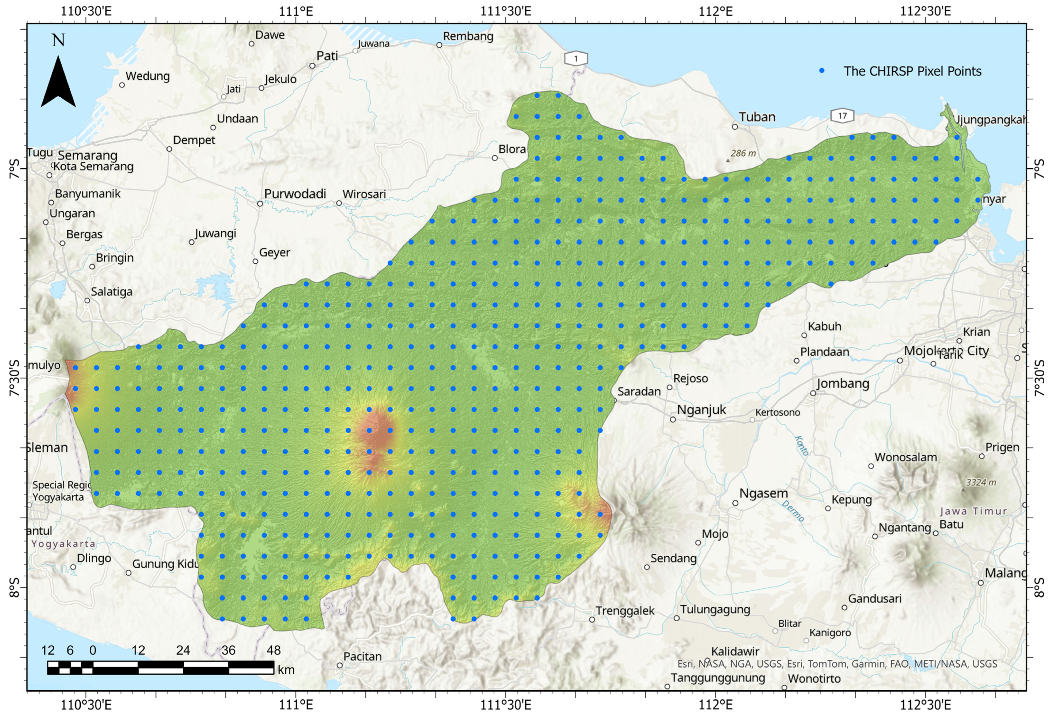
To ensure representative spatial coverage across the entire study area, namely the Bengawan Solo River Basin, the CHIRPS was extracted to points. This process resulted in a total of 523 points, evenly distributed within the basin boundaries. Each point represents an area of a CHIRSP pixel. Each point has a 44-year monthly rainfall time series (1981–2024), which means that each point stores 528 monthly rainfall data. This extensive dataset not only enriches the variety of rainfall patterns that prediction models can study but also enables the use of modeling techniques that require large amounts of historical data. This multidecadal data also facilitates a more robust model training and validation process, enabling the capture of long-term trends, seasonal cycles, and spatiotemporal extreme events [34]. All data were then arranged in a matrix format (CSV file), ready to be entered into the modeling workflow, both at the model training and validation stages.

2.3. Research Framework

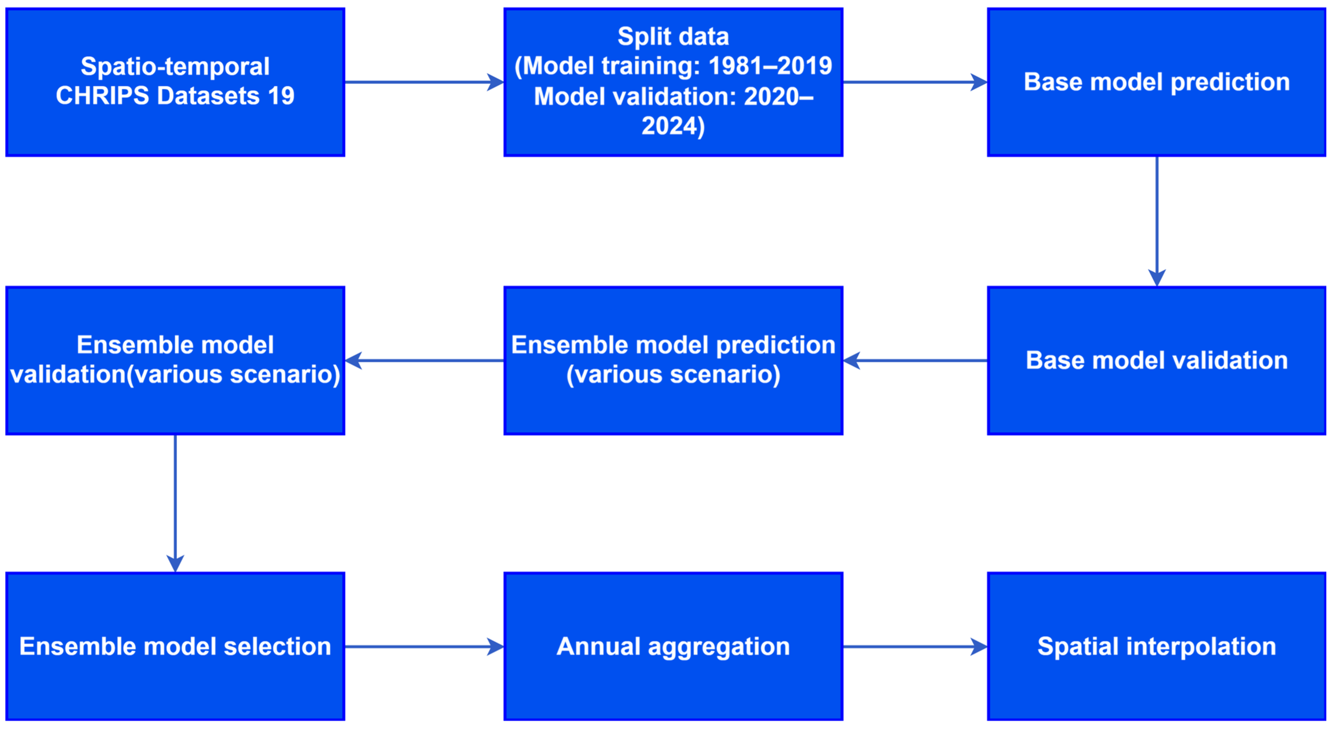
This study employs an integrated workflow based on ensemble stacking for spatiotemporal prediction of annual rainfall for the period 2025–2030 (Figure 2). This research framework begins with the collection of CHIRPS data and watershed area data, the creation of systematic spatial sampling points, the training of various rainfall prediction models (ML and DL), ensemble stacking, performance evaluation, aggregation, spatiotemporal interpolation, and evaluation and analysis to produce projected rainfall maps for 2025–2030.

2.3.1. Preprocessing

The preprocessing and data partitioning stages are important foundations in the spatiotemporal modeling workflow, especially when handling large and heterogeneous multi-point time series data from CHIRPS satellites. In this study, all monthly rainfall data extracted from 523 points in the Bengawan Solo River Basin (Figure 3) for the period 1981–2024 were organized into a two-dimensional matrix, where each row represents a single sample point and each column represents the corresponding month of observation. This data structure greatly supports analysis efficiency and is compatible with most machine learning and deep learning architectures.
The first step in preprocessing is to check and handle missing values. Although CHIRPS data is generally complete, there may be missing values (NA) due to satellite anomalies or the mosaicking process. Missing values found in the sample point time series are addressed using linear interpolation or, if necessary, imputation based on local seasonal averages. This process aims to maintain the continuity of the time series to avoid interfering with the model training process, especially in sequence-based models such as LSTM and GRU, which are sensitive to missing values. The data is then divided into two main subsets based on the year of observation:
  • Training set: includes data from January 1981 to December 2019. This data is used to train the model, extract seasonal patterns and long-term trends, and tune parameters.
  • Validation set: includes data from January 2020 to December 2024. This data serves to evaluate the model’s ability to make out-of-sample predictions, thereby measuring the model’s accuracy in the most recent period.
In addition, sequence data (windowing) was also created, in which monthly rainfall data was converted into sequence segments (24 consecutive months as input, with the 25th month as the prediction target) to match the input format of the time series prediction model (e.g., LSTM, GRU, TCN). This process was systematically applied to all points, allowing the model to learn the spatiotemporal patterns of the entire study area.
Finally, all preprocessing, sequence, and data division results are documented and stored in a format compatible with the Python 3.12.12 modeling framework (NumPy 2.2.2, Pandas 2.0.2) on Google Colab Pro, allowing for the training, validation, and evaluation processes to be carried out in a reproducible and structured manner.

2.3.2. Development of Prediction Models

After the CHIRPS data in the Bengawan Solo watershed were preprocessed and divided, the next stage involved developing a spatio-temporal rainfall prediction model. This study employed a multi-model approach, in which both machine learning (ML) and deep learning (DL) models were systematically applied and evaluated to obtain a comprehensive understanding of the prediction performance.
  • Machine Learning (ML) Models
Four classic ML models were used as baselines, namely Random Forest (RF) [20], Extreme Gradient Boosting (XGB) [19], Support Vector Regression (SVR) [35], Multi-Layer Perceptron (MLP) [36], and LightGBM (LGBM) [37,38]. RF and XGB are decision tree-based ensemble models that have proven effective for non-linear data, capturing interactions between features well. SVR offers a flexible kernel approach to map non-linear input-output relationships. At the same time, MLP represents a simple neural network with complex feature learning capabilities, although not as complex as DL. All of these models are implemented using the scikit-learn and xgboost libraries, with hyperparameter tuning performed using grid search and cross-validation on the training data.
2.
Deep Learning (DL) Models
Five DL architectures (Table 1) were used: LSTM [39], GRU [40], TCN [19], CNN [41], and Transformer [42]. LSTM and GRU models excel at capturing long-term dependencies in rainfall time series data, making them highly effective for seasonal patterns or long-term trends. TCN offers advantages in modeling sequence data through dilated causal convolution, which makes it efficient for spatiotemporal prediction. CNN, commonly used for spatial and image data, is applied to monthly data sequences to extract local patterns in time sequences. Meanwhile, Transformers—which are on the rise in the field of sequence modeling enable attention mechanisms that are effective in capturing spatial and temporal relationships in multi-point rainfall data.
All DL models were implemented using the TensorFlow and Keras frameworks. The input to each model was a sequence window for predicting the following month’s rainfall. The models were trained on training data (1981–2019) for each point in parallel. Training was performed with early stopping and cross-validation to avoid overfitting.
3.
Prediction and Evaluation Process
After training, each model was used to perform recursive predictions on the validation period (2020–2024) and the projection period (2025–2030). For each month, the model input is updated with the latest predictions, simulating real-world time series predictions (rolling forecast). Predictions from each base model are evaluated based on MAE, RMSE, MAPE, and R2 metrics on the 2020–2024 validation data across all points. The analysis of the performance of these individual models forms the basis for determining the contribution of each model in the ensemble, as well as for understanding the advantages and limitations of each approach [26,27].

2.3.3. Ensemble Stacking and Scenario Evaluation

After training and predicting using various machine learning (ML) and deep learning (DL) base models, the next step is to apply the ensemble stacking method to improve the accuracy, stability, and robustness of spatiotemporal rainfall predictions. Ensemble stacking was chosen because it can combine the strengths of each base model (base learner), so that another model can compensate for the weaknesses of one model, and the prediction results become more optimal in aggregate [26,27,28].
Ensemble stacking is a two-level learning technique in which the output predictions from all base models are used as new features (meta-features) to be retrained on the meta-learner. In this study, the meta-learner used is non-negative least squares (NNLS), allowing for the straightforward interpretation of the contribution weight of each base model, which is always non-negative. The stacking process is carried out at each station, ensuring that the spatial sensitivity and local characteristics of the watershed are maintained. Then, a multi-scenario ensemble experiment was conducted to compare the stacking of all ML-DL models and compile various model combinations (Table 2).
Each scenario was systematically tested to gain insight into the effect of the number and type of base models on ensemble performance [28,29]. The testing was conducted during the validation period (2020–2024), allowing for the determination of which scenarios consistently produced the smallest error and the highest R2, both in aggregate and at specific points.
The evaluation metrics used were Mean Absolute Error (MAE) (Equation (1)), Root Mean Square Error (RMSE) (Equation (2)), Mean Absolute Percentage Error (MAPE) (Equation (3)), and coefficient of determination (R2) (Equation (4)). Each metric is calculated for all sample points and validation months, and visualized in the form of bar graphs, heatmaps, radar plots, and comparative tables. This evaluation also compares the performance of the ensemble with each base model, allowing for the identification of the increase in accuracy due to stacking.
M A E = 1 n i = 1 n | y i y ^ i |
R M S E = 1 n i = 1 n ( y i y ^ i ) 2
M A P E = 100 % n i = 1 n | y i y ^ i y i |
R 2 = i = 1 n ( y i y ^ i ) 2 i = 1 n ( y i y ¯ i ) 2
Furthermore, performance tests were conducted on various stacking scenarios to assess the robustness and generalizability of the ensemble framework against data variations, both at points with high and low rainfall, as well as in various validation years. Thus, the resulting prediction model recommendations are not only specific to the Bengawan Solo watershed but can also be adopted or further developed for other tropical regions with similar hydrological characteristics.

2.3.4. Data Aggregation (Monthly to Annual)

After obtaining monthly rainfall prediction results at each sample point from the model or ensemble with the best performance, the next step is to aggregate the monthly data into annual rainfall. This aggregation process is fundamental in the context of hydrology and water resource management because annual rainfall information is more relevant for planning, trend analysis, and decision-making at the macro level, such as water availability projections, flood or drought potential predictions, and watershed management policy recommendations.
Aggregation is performed by summing the monthly rainfall predictions (in millimeters) at each sample point for the period from January to December of each year, specifically for the projection years 2025 to 2030. Mathematically, for sample point i and year t, the annual rainfall P i , t y e a r is calculated as Equation (5).
P i , t y e a r = m = 1 12 P i , t , m m o n t h
Here P i , t , m m o n t h is the predicted rainfall for the month m at point i and year t.
This aggregation is performed automatically on all points in the Bengawan Solo watershed, resulting in an annual rainfall data matrix (point × year) for the 2025–2030 projection period. The use of yearly aggregation results facilitates inter-year comparisons and the identification of long-term trends, allowing for the observation of possible increases, decreases, or extreme fluctuations in rainfall that could potentially affect water management in the Bengawan Solo watershed.

2.3.5. Spatial Interpolation

After obtaining the 2025–2030 annual rainfall prediction results at all systematic sample points in the Bengawan Solo watershed area, the next step is to perform spatial interpolation to produce a yearly continuous rainfall distribution map for the entire study area. This interpolation process is crucial because the distribution of sample points cannot accurately represent all spatial variations if used discretely; a geostatistical approach is necessary to estimate rainfall values in locations where there are no direct samples.
The interpolation method used in this study is kriging, a classic spatial method widely employed in hydrology. The kriging interpolation was performed for each projection year (2025–2030), resulting in a spatial map of annual rainfall in raster form for the entire Bengawan Solo watershed. This process used the Kriging tool in ArcGIS 10.8.

2.3.6. Visualization and Analysis of Results

The final stage of this study involved visualizing and analyzing the results for both numerical predictions and spatial outputs. The main output of the spatial interpolation results was a map of annual rainfall distribution (2025–2030) presented in raster form, reflecting rainfall variations throughout the Bengawan Solo watershed. Each year’s projection is visualized separately, allowing for precise identification of changes in spatial patterns from one year to the next. The analysis of the results focuses on two main aspects: evaluating model performance and interpreting spatiotemporal patterns. In terms of model performance, a comparison is made between the results of individual models and ensembles on all evaluation metrics, as well as an analysis of the contribution of each base model in the optimal stacking scenario.

3. Results

3.1. Evaluation of Individual Model Performance

An initial model performance assessment was conducted individually for all machine learning (ML) and deep learning (DL) algorithms applied to monthly rainfall prediction (validation period: 2020–2024) at 523 points in the Bengawan Solo watershed. Table 3 summarizes the evaluation results of the primary metrics for each model.
Among single models, XGB and GRU deliver the strongest overall performance, followed closely by LGBM and RF. MLP and LSTM are mid-range (R2 ≈ 0.659–0.658; RMSE ≈ 89–90 mm), while SVR is comparable but slightly lower (MAE 66.85 mm, RMSE 90.37 mm, R2 0.652). Deep architectures, such as TCN, CNN, and Transformer, underperform on these monthly series (R2 ≈ 0.51, 0.40, 0.42; with higher errors).

3.2. Analysis of Ensemble Stacking Performance in Various Scenarios

After evaluating the performance of individual models, the next step is to analyze the results of ensemble stacking with various combinations of base learners. A total of 17 ensemble stacking scenarios were designed, representing different combinations of machine learning (ML) and deep learning (DL) base models, ranging from ML-only and DL-only models to ML–DL combinations and all models at once (see Table 4).

3.3. Comparative Analysis Between Scenarios

Based on the results in the table above (Table 4), the best overall ensembles are Q (10 models), J (9), and F (8)—all essentially tied—with Q very slightly ahead (MAE 53.73 mm; RMSE 69.20 mm; MAPE 57.61%; R2 0.7961), followed by J (53.82; 69.33; 57.95%; 0.7953) and F (53.83; 69.33; 57.99%; 0.7953). Adding models beyond a diverse ML-led mix yields diminishing returns (e.g., from D: RMSE 70.22; R2 0.7900 to Q: RMSE 69.20; R2 0.7961). Ensembles dominated by traditional ML consistently outperform simpler mixes: A/B/G/N (mostly tree/boosting + SVM/MLP) sit around MAE ≈ 58.2–58.4 mm, RMSE ≈ 74.75–74.98 mm, R2 ≈ 0.760–0.762.
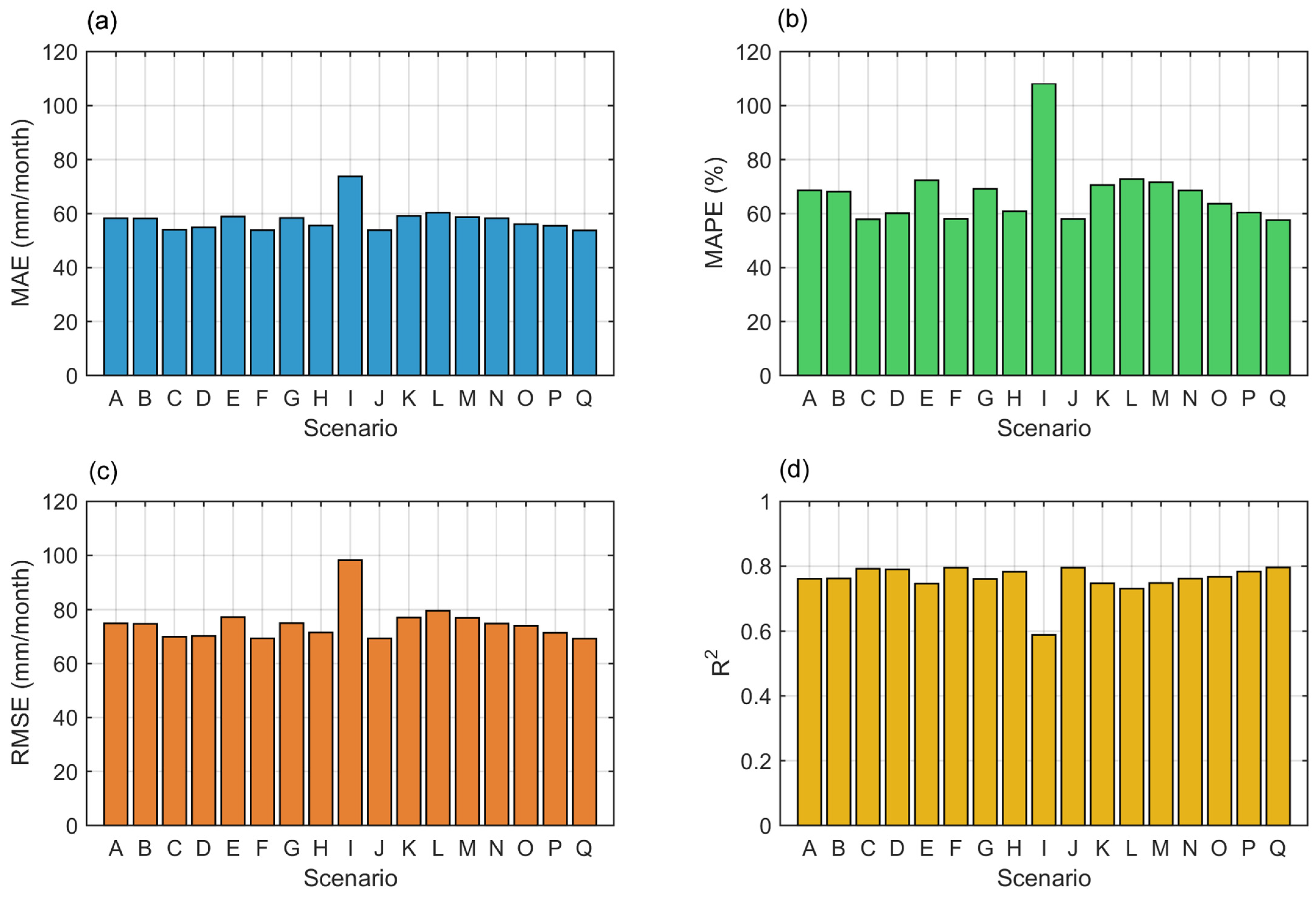
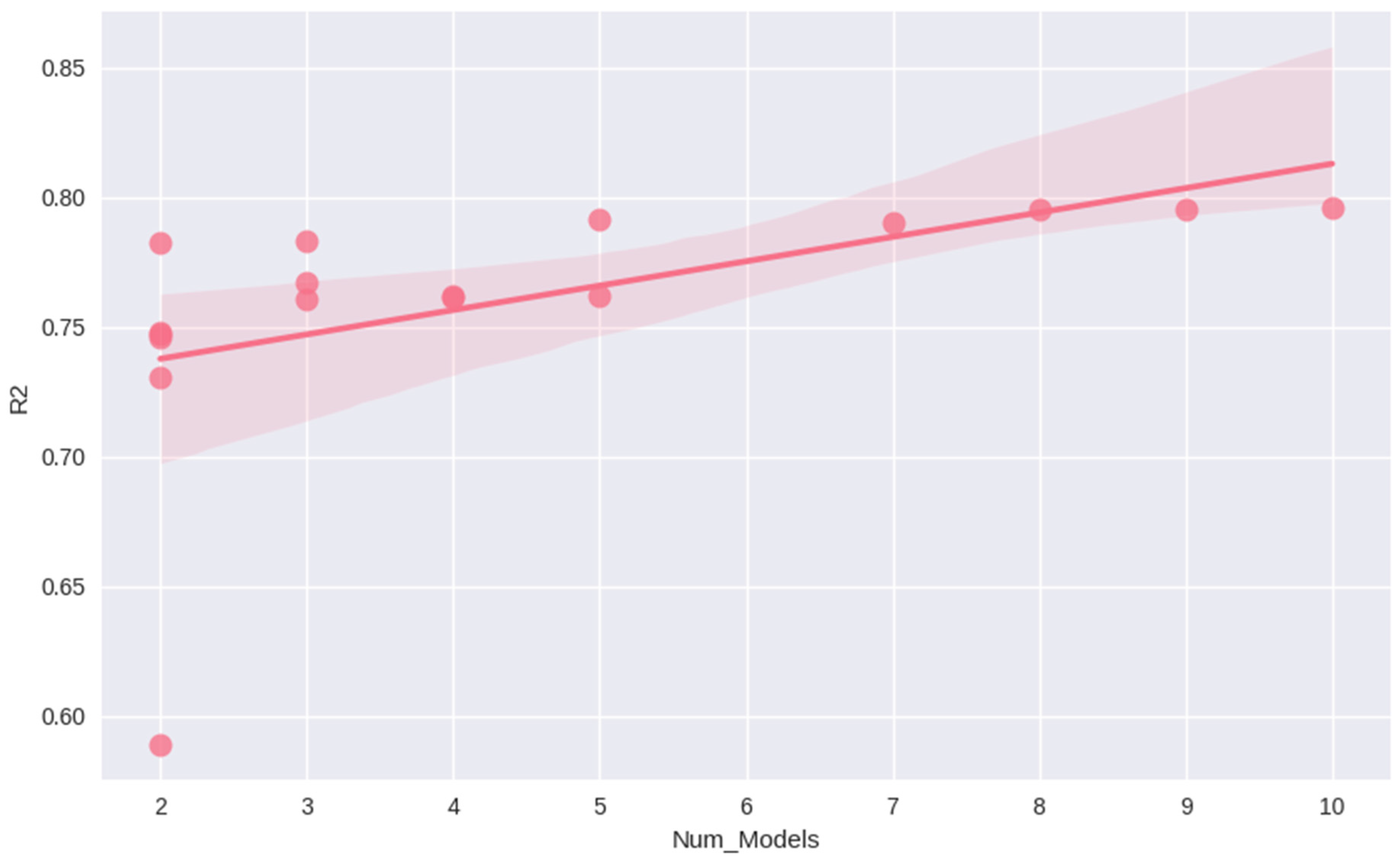
Notably, the DL-only five-model stack (C) is competitive (MAE 54.03; RMSE 69.94; MAPE 57.87%; R2 0.7917) but still trails Q/J/F. Minor or DL-heavy pairs/triads fare worse: H (LSTM+GRU) and P (MLP+LSTM+GRU) are mid-range (R2 ≈ 0.782), while two-model mixes E/K/L/M underperform (R2 ≈ 0.73–0.75). The CNN+Transformer pair (I) performs poorly (MAE 133.53; RMSE 154.00; MAPE 279.01%; R2 0.0443). Overall, broad, ML-anchored ensembles deliver the most reliable accuracy, and incorporating weaker DL bases (e.g., CNN, Transformer) does not improve—and can degrade—stack performance unless balanced by stronger learners. Figure 4, Figure 5 and Figure 6 provide a comparison of the performance of all scenarios.
Figure 4, the bar plot of the ensemble results, illustrates a consistent pattern that the combination of traditional ML models remains the backbone in the scenarios. These results are in line with findings in the literature that stacking with strong ML base learners is more stable and robust [26,43]. The correlation between metrics (Figure 5) exhibits a consistent pattern: MAE, RMSE, and MAPE are almost perfectly correlated (≈ranging from approximately 0.99 to 1.00), while all are almost perfectly negatively correlated with R2 (≈ranging from approximately −0.99 to −1.00). This is reasonable because R2 is mathematically related to MSE/RMSE (R2 = 1 − SSE/SST). Hence, a decrease in absolute error is almost always accompanied by an increase in R2, provided that the observation variability remains similar between scenarios. On the other hand, the number of models in the ensemble is moderately correlated with performance improvement (number of models vs. MAE/RMSE/MAPE ≈ −0.53 to −0.55; vs. R2 ≈ +0.52), indicating that adding diversity to the base learner generally improves accuracy but with diminishing returns after a certain point (Figure 6).

3.4. Spatial and Temporal Error Analysis

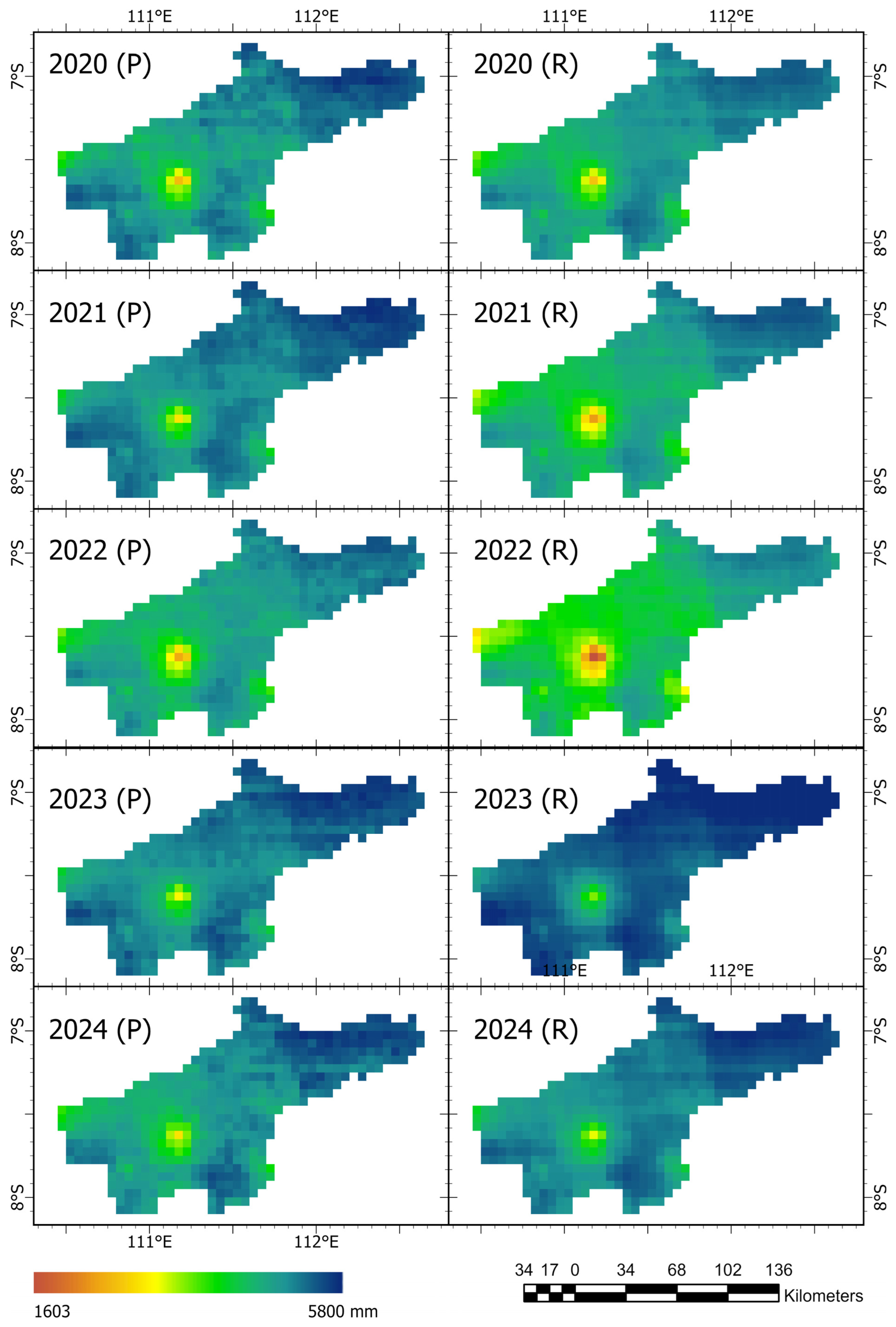
The evaluation of rainfall prediction model performance is not only conducted in aggregate, but also spatially (between sample points) and temporally (between months). This approach is crucial for understanding the stability, fairness, and limitations of predictions in various contexts and time periods within the study area. Visually (Figure 7), a comparison of the predicted rainfall series and map (P) with CHIRPS observations (R) shows strong spatial-seasonal coherence: the peak of the rainy season and the minimum of the dry season occur at similar times and locations in most watersheds, so that the patterns of P and R appear qualitatively similar.
Quantitatively, based on 17 scenarios (A–Q) and 523 points in the 2020–2024 validation period, the error pattern shows strong spatiotemporal consistency. Spatially, absolute error increases in sloped/elevated zones (strong positive MAE–elevation and RMSE–elevation correlations), while MAPE decreases at higher elevations (greater rainfall base suppresses percentage error) and R2 increases slightly—reflecting the influence of orographic/convective complexity (topographic gradient, rain shadow, microclimate). Low MAE points appear more frequently in the middle zone of the watershed and in areas with moderate seasonal variability; high MAE is concentrated downstream and at the edges of the watershed where hydro-atmospheric dynamics are more extreme and the potential for remote sensing bias is greater. Temporally, the cross-scenario error series consistently peaks during the transition months (March–April; October–November) and the peak of the rainy season (around Dec–Feb), when convective events/sub-daily intensities are difficult to capture with monthly resolution; conversely, the dry season (±June–September) shows lower and more stable errors. This phenomenon is often an obstacle to hydrological prediction in tropical regions [44]. This pattern is robust across all scenarios: the best ensemble (Q/J/F) reduces the error level but does not alter the spatial distribution or seasonal rhythm; outliers persist in highly localized rainfall events or seasonal shifts that are not fully captured by the observation network. The implication is that improving accuracy needs to prioritize orographic zones and transition periods, for example, through pre-processing sharpening (CHIRPS bias-correction), large-scale climate features, or more adaptive temporal windows.

3.5. Analysis of Spatio-Temporal Rainfall Patterns

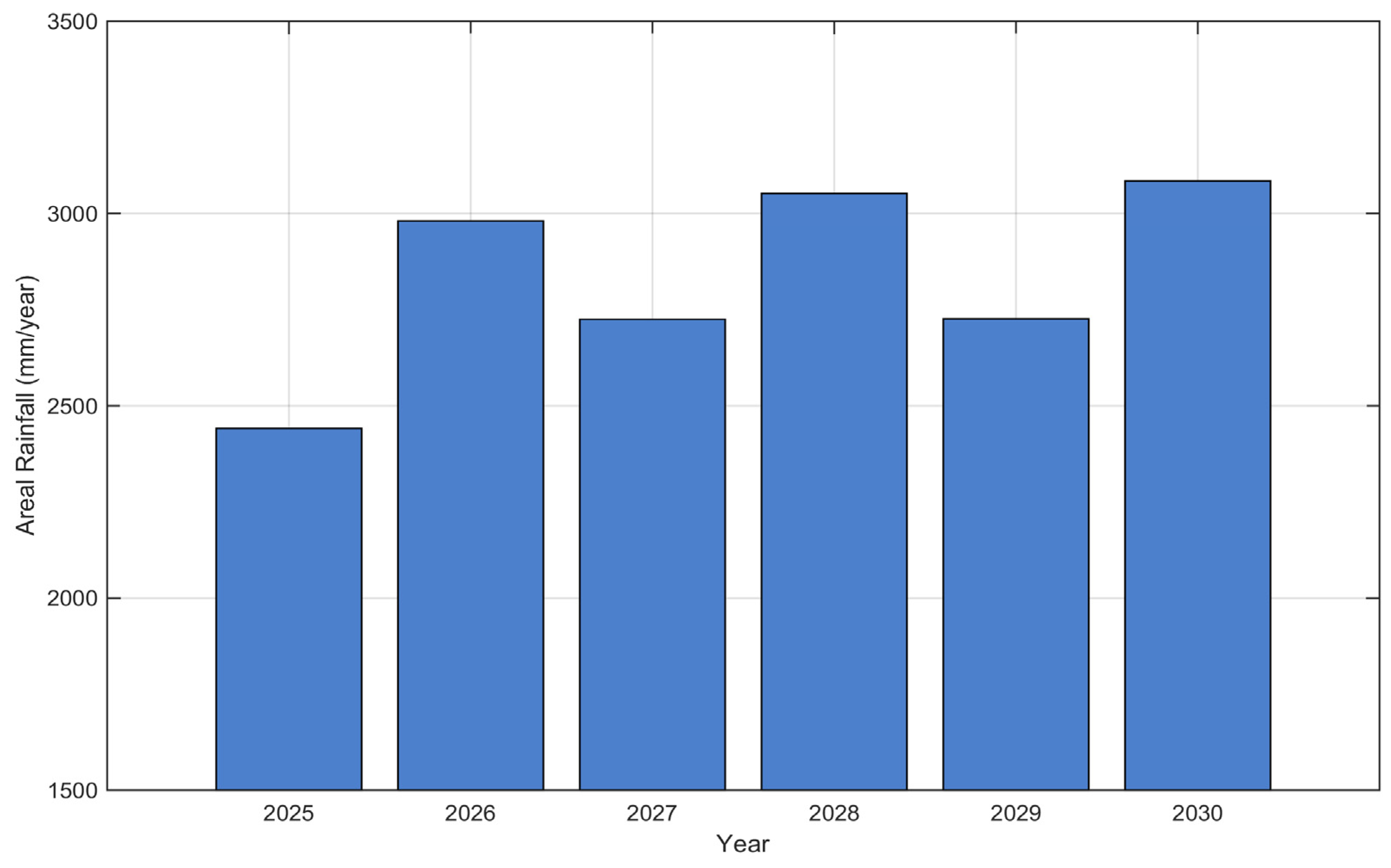
The results of the annual average analysis show considerable fluctuations in rainfall in the Bengawan Solo River Basin during the period 2025–2030. These results reveal that the highest rainfall is projected to occur in 2028 with an average value of around 2763 mm, followed by 2758 mm in 2030. Meanwhile, the lowest rainfall is expected to appear in 2025, with a value of around 2326 mm, which is higher than the initial estimates. This pattern exhibits significant interannual variability, which is likely related to global climate phenomena such as El Niño and La Niña, which have historically influenced the intensity and distribution of rainfall in tropical Indonesia. The sharp increase from 2025 to 2026, followed by fluctuations in subsequent years, confirms the existence of a fluctuating natural climate cycle. Understanding this pattern is crucial to consider when developing strategies to mitigate the risks of flooding and drought (Figure 8).
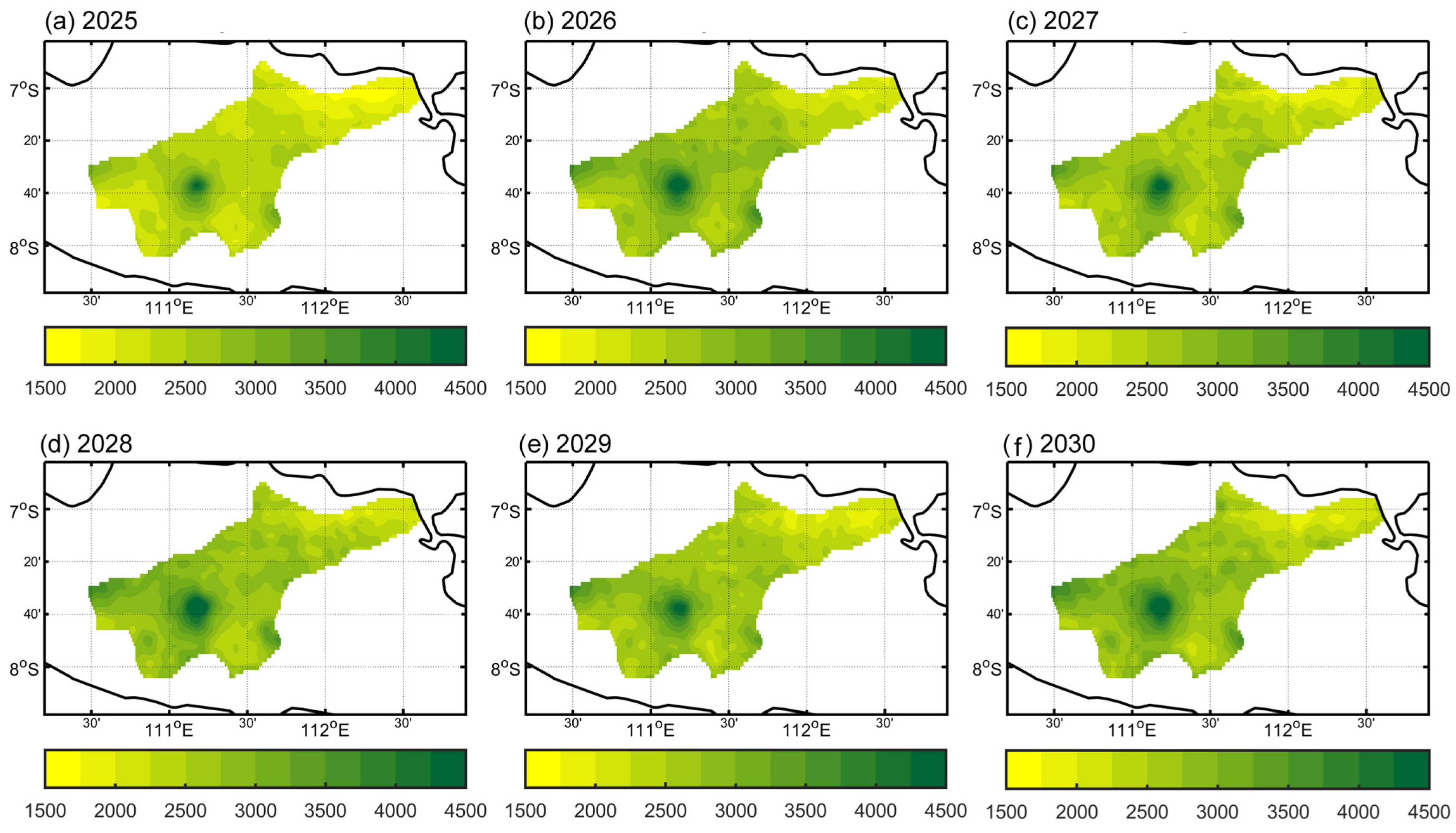
Spatially, the average rainfall distribution during 2025–2030 is not homogeneous across the watershed (Figure 9). The northern and western regions, especially those close to the Merapi, Merbabu, and Lawu mountains, exhibit higher rainfall (up to 2600 mm), while the southern and eastern areas tend to be drier, with values around 2000 mm. This spatial pattern is consistent with the orographic characteristics of the Bengawan Solo watershed, where topography causes differences in rainfall intensity. The existence of areas with higher rainfall indicates a potential for large runoff and an increased risk of flooding in downstream areas, while areas with lower rainfall may face challenges in water availability during the dry season.
The temporal fluctuations do not occur evenly across all locations. Areas with high rainfall consistently dominate the spatial pattern, although the intensity decreases in dry years. This shows that temporal variability exacerbates spatial disparities: in dry years, wet areas continue to receive relatively high rainfall, while dry areas are further stressed. These conditions can exacerbate the inequality of water resource distribution, posing the risk of flooding on one side and drought on the other. These findings support the application of prediction models based on ensemble machine learning and deep learning because they can capture complex spatial and temporal heterogeneity.

4. Discussion

4.1. Evaluation of Findings

This study clearly found that the ensemble stacking framework, which combines traditional machine learning models (RF, XGB, SVR, MLP) and deep learning models (LSTM, GRU, TCN, CNN, Transformer), can provide higher accuracy in predicting annual spatiotemporal rainfall in the Bengawan Solo River Basin than individual models. This study successfully answers the main question regarding the effectiveness of the ensemble method in CHIRPS data-based rainfall prediction (Figure 9). This key finding reinforces the argument that no single model can dominate in all cases, making the integration of various models through ensemble stacking a valuable strategy. In this study, the strongest contributions came from ML models, while DL architectures showed limited performance due to data and complexity constraints. Practically, the success of stacking lies in combining the best-performing ML models to achieve more stable and robust rainfall predictions than any single approach.
Consistent with that setting, correlation analyses across 523 stations (Table 5) show that absolute errors rise with altitude (Figure 10): RMSE and MAE are strongly and positively correlated with elevation (r ≈ 0.69 and 0.72, both p < 0.001), with error gradients of about +1.99 mm RMSE and +1.78 mm MAE per +100 m. This pattern is consistent with increasing orographic complexity (e.g., convective enhancement, rain-shadow effects, and microclimate variability) that inflates absolute error in millimeters. In other words, the ML-anchored stacking approach mitigates—but cannot fully eliminate—the error floor imposed by topography, explaining both its superior overall performance and the residual elevation-linked error structure. Conversely, MAPE actually decreases with elevation (r ≈ −0.27 Pearson; ρ ≈ −0.46 Spearman; p < 0.001), thereby reducing relative error. R2 increases slightly with elevation, indicating that the ability to explain variation does not deteriorate, even though the absolute error increases.
The RMSE/MAE pattern increases with elevation, but the decrease in MAPE can be explained by orographic complexity: high areas tend to have more intense/variable rainfall, resulting in larger absolute errors (mm), while the larger rainfall base suppresses percentage errors. Previous studies on highlands have shown spatial and temporal heterogeneity, as well as a shift towards moderate to heavy rainfall on mountain slopes [45], which is consistent with monsoonal contexts, such as the Bengawan Solo. In terms of time, sub-daily irregularities—especially in transitional seasons—make convective episodes difficult for models to capture and explain the peaks in error during transitional months [46]. Because the hydrological–ecological response is sensitive to the temporal structure of rainfall (i.e., timing, duration, and intensity), biases in capturing rainfall timing patterns can directly affect operational decisions and management strategies (e.g., early warnings, water resource allocation) [47]. Furthermore, the co-occurrence of precipitation and water vapor transport extremes in complex topography adds statistical challenges and can degrade sequential model performance during months of extreme rainfall [48]. Overall, the combination of orography, convective variability, and teleconnections explains the elevation gradient of error and underscores the importance of seasonally and extremely sensitive evaluations, while the decrease in MAPE at high elevations is consistent with larger denominators (rainfall).
These findings are very important, both theoretically and practically. Theoretically, the success of stacking demonstrates that machine learning and deep learning models capture distinct spatiotemporal patterns of rainfall, resulting in more stable and robust estimates when combined. This is crucial for reducing model bias risk and anticipating local climate variability, particularly in tropical regions characterized by highly complex atmospheric dynamics. Practically, this improvement in prediction accuracy has a significant impact on water resource planning and management, disaster risk mitigation, and the formulation of climate change adaptation policies in the Bengawan Solo River Basin. With the ensemble stacking model, rainfall projections for the 2025–2030 period become more reliable and can serve as a reference for informed decision-making.
The results of this study are consistent with those of various recent studies, which also found that the ensemble stacking approach consistently outperforms individual base models. Papacharalampous et al. [26] and El Hafyani et al. [28] demonstrated that stacking can significantly reduce error values (RMSE, MAE) and increase R2 values in spatiotemporal rainfall predictions. Other studies also report improved model generalization in regions with minimal data or complex topography [27,43], as well as prediction stability across seasons and rainfall intensity levels [49]. This study reinforces this consensus while expanding the scope of the experiment by testing dozens of stacking combinations on long-term CHIRPS data in large tropical watersheds.

4.2. Limitations and Future Works

However, several limitations should be noted. First, although stacking improves aggregate performance, spatial analysis reveals points with high errors at watershed boundaries, particularly in locations with unique microclimatic and topographic conditions. Second, predictions during transitional months or extreme rainfall events remain a significant challenge due to high atmospheric uncertainty, CHIRPS input bias, and the model’s temporal resolution limitations. Additionally, the stacking approach used is still based on a simple meta-learner (positive linear regression); exploration of non-linear meta-learners may provide further improvements.
To that end, Several future research agendas can be developed to strengthen this framework. First, priority should be given to integrating the ENSO [50], IOD [51], and MJO [52] indices, as explanatory variables in the base models. This integration would improve the spatiotemporal representation of rainfall variability and reduce errors, especially at extreme values. Second, the exploration of deep learning-based meta-learners, adaptive weighting, or even multi-level stacking (multi-layer ensemble) is worth investigating [53]. Third, generalizing the framework to other watersheds in Indonesia and Southeast Asia, as well as validating it using field observation data, is crucial to demonstrate the robustness and transferability of the results. In addition, the development of a hydrological early warning system based on spatiotemporal ensemble prediction will be a valuable practical contribution in the future.
This study confirms and extends current knowledge by demonstrating the superiority of ensemble stacking for spatio-temporal rainfall prediction. Through multi-scenario comparisons, broad spatial and temporal coverage, and empirical validation using CHIRPS data in tropical regions, it provides robust evidence of the effectiveness of stacking. The findings have significant implications for disaster mitigation, water resource management, and climate adaptation, offering a scalable framework to strengthen resilience in tropical regions.

5. Conclusions

The CHIRPS-based rainfall prediction framework with ensemble stacking in the Bengawan Solo watershed consistently outperforms single models. In the 2020–2024 validation, the best performance was achieved by Scenario Q (10 models) with an RMSE of 69.20 mm and R2 of 0.796 (MAE 53.73 mm; MAPE 57.61%), closely followed by Scenario J (9) and F (8) (RMSE ≈ 69.33 mm; R2 ≈ 0.795). Scenario C (DL-only: LSTM, GRU, TCN, CNN, Transformer) was competitive (RMSE 69.94; R2 0.792), but still below Q/J/F. In contrast, small ML-based ensembles such as A/B/G/N (RMSE ≈ 74.75–74.98; R2 ≈ 0.761) are stable but weaker. The combination of two models (E/K/L/M) and the CNN-Transformer pair (I) yields the lowest performance (I: RMSE 98.27; MAPE 108.22; R2 0.589). These findings confirm that diverse ensembles anchored to strong ML models provide the most consistent accuracy, while adding weak DL base learners does not improve—and may even degrade—performance. Increasing the number of models also shows diminishing returns once the core ML portfolio is fully represented.
Spatially–seasonally, stacking most consistently replicates topography–monsoon patterns and extreme fluctuations compared to single models. Orographic analysis shows RMSE/MAE increase with elevation (Pearson r ≈ 0.689/0.716, p < 0.001; gradient ≈ +1.99 mm RMSE and +1.78 mm MAE per +100 m), MAPE decreased (r ≈ −0.274, p < 0.001), and R2 slightly increased (r ≈ 0.171, p < 0.001). Physically, this is consistent with orographic/convective complexity amplifying absolute error (mm), while greater rainfall intensity at higher elevations suppresses percentage error. We posit the lower performance of DL as a hypothesis related to capacity–data matching and sub-seasonal dynamics that are difficult to capture within a monthly window. Since simpler DL variants have not been tested in this study, this statement does not constitute a causal conclusion.
This study has demonstrated that the ensemble stacking approach, which combines various machine learning and deep learning models, can significantly enhance the accuracy of spatiotemporal rainfall predictions in the Bengawan Solo River Basin. By utilizing long-term CHIRPS data and various model combination scenarios, this study’s results emphasize the importance of integrating classical and modern models to address the challenge of hydrometeorological prediction in complex tropical regions. In addition to offering improved performance, this method also demonstrates resilience in the face of high spatial and temporal variability.
Beyond method advances, the study’s implications are far-reaching: more accurate rainfall forecasts can directly support early warning systems, strengthen disaster preparedness, and optimize water resource allocation in flood- and drought-prone regions. By bridging machine learning and deep learning within an ensemble framework, this work provides a scalable blueprint for enhancing climate resilience in tropical basins, with potential applications across Southeast Asia and other vulnerable regions worldwide.

Author Contributions

Conceptualization, J.J., D.D., E.R. and A.U.; methodology, J.J.; software, J.J.; validation, J.J.; formal analysis, J.J.; writing—original draft preparation, J.J., D.D., E.R., A.U., S.S., L.K.C., F.S. and M.N.; writing—review and editing, J.J., D.D., E.R., A.U., S.S., L.K.C., F.S. and M.N.; visualization: J.J.; funding acquisition, J.J. and M.N. All authors have read and agreed to the published version of the manuscript.

Funding

This research was funded by DPPM Kemdiktisaintek RI, grant number 0419/C3/DT.05.00/2025, 127/C3/DT.05.00/PL/2025, 0070/C3/AL.04/2025, 007/LL6/PL/AL.04/2025, 168.30/A.3-III/LRI/VI/2025.

Data Availability Statement

The data presented in the study are openly available supporting information can be downloaded at https://doi.org/10.17605/OSF.IO/YTZA6.

Acknowledgments

We would like to acknowledge DPPM Kemendikbudristek RI for funding. During the preparation of this manuscript/study, the author(s) used Gemini and ChatGPT 5 for the purpose of code and text editing. The authors have reviewed and edited the output and take full responsibility for the content of this publication.

Conflicts of Interest

The authors declare no conflicts of interest.

References

  1. Funk, C.; Peterson, P.; Landsfeld, M.; Pedreros, D.; Verdin, J.; Shukla, S.; Husak, G.; Rowland, J.; Harrison, L.; Hoell, A. The Climate Hazards Infrared Precipitation with Stations—A New Environmental Record for Monitoring Extremes. Sci. Data 2015, 2, 150066. [Google Scholar] [CrossRef]
  2. Alikhanov, B.; Pulatov, B.; Samiev, L. Impact of Climate Change on the Cryosphere of the Ugam Chatkal National Park, Bostonliq District, Uzbekistan, During the Post-Soviet Period, Based on Remote Sensing and Statistical Analysis. Forum Geogr. 2024, 38, 302–316. [Google Scholar] [CrossRef]
  3. Haq, D.Z.; Novitasari, D.C.R.; Hamid, A.; Ulinnuha, N.; Farida, Y.; Nugraheni, R.D.; Nariswari, R.; Rohayani, H.; Pramulya, R.; Widjayanto, A. Long Short-Term Memory Algorithm for Rainfall Prediction Based on El-Nino and IOD Data. Procedia Comput. Sci. 2021, 179, 829–837. [Google Scholar] [CrossRef]
  4. Ward, P.J.; Van Pelt, S.C.; De Keizer, O.; Aerts, J.C.J.H.; Beersma, J.J.; Van Den Hurk, B.J.J.M.; Te Linde, A.H. Including Climate Change Projections in Probabilistic Flood Risk Assessment. J. Flood Risk Manag. 2014, 7, 141–151. [Google Scholar] [CrossRef]
  5. Kasihairani, D.; Hidayat, R.; Supari, S. Assessing the Reliability of Predicted Decadal Surface Temperatures in Southeast Asia. Forum Geogr. 2024, 38, 413–425. [Google Scholar] [CrossRef]
  6. Winsemius, H.C.; Aerts, J.C.; Van Beek, L.P.; Bierkens, M.F.; Bouwman, A.; Jongman, B.; Kwadijk, J.C.; Ligtvoet, W.; Lucas, P.L.; Van Vuuren, D.P. Global Drivers of Future River Flood Risk. Nat. Clim. Change 2016, 6, 381–385. [Google Scholar] [CrossRef]
  7. Gu, J.; Liu, S.; Zhou, Z.; Chalov, S.R.; Zhuang, Q. A Stacking Ensemble Learning Model for Monthly Rainfall Prediction in the Taihu Basin, China. Water 2022, 14, 492. [Google Scholar] [CrossRef]
  8. Praveen, B.; Talukdar, S.; Shahfahad; Mahato, S.; Mondal, J.; Sharma, P.; Islam, A.R.M.T.; Rahman, A. Analyzing Trend and Forecasting of Rainfall Changes in India Using Non-Parametrical and Machine Learning Approaches. Sci. Rep. 2020, 10, 10342. [Google Scholar] [CrossRef]
  9. Schaffer, A.L.; Dobbins, T.A.; Pearson, S.-A. Interrupted Time Series Analysis Using Autoregressive Integrated Moving Average (ARIMA) Models: A Guide for Evaluating Large-Scale Health Interventions. BMC Med. Res. Methodol. 2021, 21, 58. [Google Scholar] [CrossRef] [PubMed]
  10. Chen, C.; Zhang, Q.; Kashani, M.H.; Jun, C.; Bateni, S.M.; Band, S.S.; Dash, S.S.; Chau, K.-W. Forecast of Rainfall Distribution Based on Fixed Sliding Window Long Short-Term Memory. Eng. Appl. Comput. Fluid Mech. 2022, 16, 248–261. [Google Scholar] [CrossRef]
  11. Ni, L.; Wang, D.; Singh, V.P.; Wu, J.; Wang, Y.; Tao, Y.; Zhang, J. Streamflow and Rainfall Forecasting by Two Long Short-Term Memory-Based Models. J. Hydrol. 2020, 583, 124296. [Google Scholar] [CrossRef]
  12. Hu, C.; Wu, Q.; Li, H.; Jian, S.; Li, N.; Lou, Z. Deep Learning with a Long Short-Term Memory Networks Approach for Rainfall-Runoff Simulation. Water 2018, 10, 1543. [Google Scholar] [CrossRef]
  13. Miao, Q.; Pan, B.; Wang, H.; Hsu, K.; Sorooshian, S. Improving Monsoon Precipitation Prediction Using Combined Convolutional and Long Short Term Memory Neural Network. Water 2019, 11, 977. [Google Scholar] [CrossRef]
  14. Fang, L.; Shao, D. Application of Long Short-Term Memory (LSTM) on the Prediction of Rainfall-Runoff in Karst Area. Front. Phys. 2022, 9, 790687. [Google Scholar] [CrossRef]
  15. Shi, X.; Chen, Z.; Wang, H.; Yeung, D.-Y.; Wong, W.-K.; Woo, W. Convolutional LSTM Network: A Machine Learning Approach for Precipitation Nowcasting. Adv. Neural Inf. Process. Syst. 2015, 28, 1–9. [Google Scholar]
  16. Slater, L.J.; Arnal, L.; Boucher, M.-A.; Chang, A.Y.-Y.; Moulds, S.; Murphy, C.; Nearing, G.; Shalev, G.; Shen, C.; Speight, L. Hybrid Forecasting: Blending Climate Predictions with AI Models. Hydrol. Earth Syst. Sci. 2023, 27, 1865–1889. [Google Scholar] [CrossRef]
  17. Espeholt, L.; Agrawal, S.; Sønderby, C.; Kumar, M.; Heek, J.; Bromberg, C.; Gazen, C.; Carver, R.; Andrychowicz, M.; Hickey, J. Deep Learning for Twelve Hour Precipitation Forecasts. Nat. Commun. 2022, 13, 5145. [Google Scholar] [CrossRef]
  18. Koya, S.R.; Roy, T. Temporal Fusion Transformers for Streamflow Prediction: Value of Combining Attention with Recurrence. J. Hydrol. 2024, 637, 131301. [Google Scholar] [CrossRef]
  19. Lim, B.; Zohren, S. Time-Series Forecasting with Deep Learning: A Survey. Philos. Trans. R. Soc. Math. Phys. Eng. Sci. 2021, 379, 20200209. [Google Scholar] [CrossRef]
  20. Laptev, N.; Yosinski, J.; Li, L.E.; Smyl, S. Time-Series Extreme Event Forecasting with Neural Networks at Uber. In Proceedings of the International conference on machine learning, Sydney, Australia, 6–11 August 2017; Volume 34, pp. 1–5. [Google Scholar]
  21. Avand, M.; Moradi, H.R.; Ramazanzadeh Lasboyee, M. Spatial Prediction of Future Flood Risk: An Approach to the Effects of Climate Change. Geosciences 2021, 11, 25. [Google Scholar] [CrossRef]
  22. Willard, J.; Jia, X.; Xu, S.; Steinbach, M.; Kumar, V. Integrating Physics-Based Modeling with Machine Learning: A Survey. arXiv 2020, arXiv:2003.04919. [Google Scholar]
  23. Kundu, S.; Biswas, S.K.; Tripathi, D.; Karmakar, R.; Majumdar, S.; Mandal, S. A Review on Rainfall Forecasting Using Ensemble Learning Techniques. E-Prime-Adv. Electr. Eng. Electron. Energy 2023, 6, 100296. [Google Scholar] [CrossRef]
  24. Nelson, B.K. Time Series Analysis Using Autoregressive Integrated Moving Average (ARIMA) Models. Acad. Emerg. Med. 1998, 5, 739–744. [Google Scholar] [CrossRef] [PubMed]
  25. Das, P.; Posch, A.; Barber, N.; Hicks, M.; Duffy, K.; Vandal, T.; Singh, D.; van Werkhoven, K.; Ganguly, A.R. Hybrid Physics-AI Outperforms Numerical Weather Prediction for Extreme Precipitation Nowcasting. npj Clim. Atmos. Sci. 2024, 7, 282. [Google Scholar] [CrossRef]
  26. Papacharalampous, G.; Tyralis, H.; Doulamis, N.; Doulamis, A. Ensemble Learning for Uncertainty Estimation with Application to the Correction of Satellite Precipitation Products. Mach. Learn. Earth 2025, 1, 015004. [Google Scholar] [CrossRef]
  27. Baig, F.; Ali, L.; Faiz, M.A.; Chen, H.; Sherif, M. How Accurate Are the Machine Learning Models in Improving Monthly Rainfall Prediction in Hyper Arid Environment? J. Hydrol. 2024, 633, 131040. [Google Scholar] [CrossRef]
  28. El Hafyani, M.; El Himdi, K.; El Adlouni, S.-E. Improving Monthly Precipitation Prediction Accuracy Using Machine Learning Models: A Multi-View Stacking Learning Technique. Front. Water 2024, 6, 1378598. [Google Scholar] [CrossRef]
  29. Shetty, S.; Dharmendra, D.; Bankapur, S.; Prasad, P. HydroStack: A Hybrid Meta-Ensemble Machine Learning Framework for Accurate Annual Rainfall Prediction. In Proceedings of the 2024 8th International Conference on I-SMAC (IoT in Social, Mobile, Analytics and Cloud)(I-SMAC), Biratnagar, Nepal, 3–5 October 2024; IEEE: Piscataway, NJ, USA, 2024; pp. 1926–1934. [Google Scholar]
  30. Kim, S.; Shin, J.-Y.; Heo, J.-H. Assessment of Future Rainfall Quantile Changes in South Korea Based on a CMIP6 Multi-Model Ensemble. Water 2025, 17, 894. [Google Scholar] [CrossRef]
  31. Priyana, Y.; Jumadi; Anna, A.N.; Rudiyanto. Farmer’s Adaptation Strategies in Facing Drought Disasters (A Case Study in Some Areas of Bengawan Solo Watershed). AIP Conf. Proc. 2023, 2727, 050026. [Google Scholar] [CrossRef]
  32. Anna, A.N.; Priyana, Y.; Rudiyanto; Fikriyah, V.N. Water Resources Management Model Based Area (A Case Study in Some Areas of Bengawan Solo Watershed). AIP Conf. Proc. 2023, 2727, 050027. [Google Scholar] [CrossRef]
  33. CHIRPS: Rainfall Estimates from Rain Gauge and Satellite Observations. Climate Hazards Center-UC Santa Barbara. Available online: https://www.chc.ucsb.edu/data/chirps (accessed on 30 August 2025).
  34. Jana, R.; Jana, N.C. Agricultural Vulnerability to Cyclones in Coastal West Bengal. DYSONA-Appl. Sci. 2026, 7, 61–72. [Google Scholar] [CrossRef]
  35. Naik, R.; Majhi, B. Explainable AI Reverse Verification Approach for Monthly Rainfall Prediction in Chhattisgarh, India. Theor. Appl. Climatol. 2025, 156, 412. [Google Scholar] [CrossRef]
  36. Kumar, V.; Kedam, N.; Kisi, O.; Alsulamy, S.; Khedher, K.M.; Salem, M.A. A Comparative Study of Machine Learning Models for Daily and Weekly Rainfall Forecasting. Water Resour. Manag. 2025, 39, 271–290. [Google Scholar] [CrossRef]
  37. Banik, R.; Biswas, A. Rainfall Prediction for Climate-Resilient Agriculture: A Robust Ensemble with SARIMA and LightGBM. Paddy Water Environ. 2025, 23, 263–275. [Google Scholar] [CrossRef]
  38. Zhuang, H.; Lehner, F.; DeGaetano, A.T. Improved Diagnosis of Precipitation Type with LightGBM Machine Learning. J. Appl. Meteorol. Climatol. 2024, 63, 437–453. [Google Scholar] [CrossRef]
  39. Pan, X.; Hou, J.; Gao, X.; Chen, G.; Li, D.; Imran, M.; Li, X.; Yang, N.; Ma, M.; Zhou, X. LSTM Model-Based Rapid Prediction Method of Urban Inundation with Rainfall Time Series. Water Resour. Manag. 2025, 39, 661–688. [Google Scholar] [CrossRef]
  40. Sivadasan, E.T.; Sundaram, N.M.; Santhosh, R. Deep Learning for Energy Forecasting Using Gated Recurrent Units and Long Short-Term Memory. J. Intell. Syst. Internet Things 2025, 14, 90. [Google Scholar] [CrossRef]
  41. Al-Samrraie, L.A.; Abdalla, A.M.; Alrawashdeh, K.A.-B.; Bsoul, A.A.; Awad, M.A.; Alzboon, K.; Al-Taani, A.A. Deep Learning Models Based on CNN, RNN, and LSTM for Rainfall Forecasting: Jordan as a Case Study. Math. Model. Eng. Probl. 2025, 12, 2456. [Google Scholar] [CrossRef]
  42. Yin, W.; Zhou, C.; Tian, Y.; Qiu, H.; Zhang, W.; Chen, H.; Liu, P.; Zhao, Q.; Kong, J.; Yao, Y. Accurate Rainfall Prediction Using GNSS PWV Based on Pre-Trained Transformer Model. Remote Sens. 2025, 17, 2023. [Google Scholar] [CrossRef]
  43. Zandi, O.; Zahraie, B.; Nasseri, M.; Behrangi, A. Stacking Machine Learning Models versus a Locally Weighted Linear Model to Generate High-Resolution Monthly Precipitation over a Topographically Complex Area. Atmos. Res. 2022, 272, 106159. [Google Scholar] [CrossRef]
  44. Zhou, Y.; Cui, Z.; Lin, K.; Sheng, S.; Chen, H.; Guo, S.; Xu, C.-Y. Short-Term Flood Probability Density Forecasting Using a Conceptual Hydrological Model with Machine Learning Techniques. J. Hydrol. 2022, 604, 127255. [Google Scholar] [CrossRef]
  45. Lu, H.; Li, F.; Gong, T.; Gao, Y.; Li, J.; Wang, G.; Qiu, J. Temporal Variability of Precipitation over the QINGHAI-TIBETAN Plateau and Its Surrounding Areas in the Last 40 Years. Int. J. Climatol. 2023, 43, 1912–1934. [Google Scholar] [CrossRef]
  46. Lu, H.-L.; Qiu, J.; Li, M.-J.; Zuo, H.-M.; Li, J.-L.; Hu, B.X.; Li, F.-F. Temporal and Spatial Variations in the Sub-Daily Precipitation Structure over the Qinghai–Tibet Plateau (QTP). Sci. Total Environ. 2024, 915, 170153. [Google Scholar] [CrossRef]
  47. Lu, H.; Qiu, J.; Hu, B.X.; Li, F. Potential Impact of Precipitation Temporal Structure on Meteorological Drought and Vegetation Condition: A Case Study on Qinghai-Tibet Plateau. J. Hydrol. Reg. Stud. 2024, 56, 102048. [Google Scholar] [CrossRef]
  48. Sun, P.; Qiu, J.; Zhang, W.; Gao, Y.; Li, J.; Li, F. Analysis of Concurrent Extreme Precipitation and Water Vapor Events on the Tibetan Plateau: Copula-Based Probability Modeling and Atmospheric Teleconnection. J. Hydrol. 2025, 661, 133695. [Google Scholar] [CrossRef]
  49. Amini, E.; Zolfaghari, A.; Kaboli, H.; Rahimi, M. Estimation of Rainfall Erosivity Map in Areas with Limited Number of Rainfall Station (Case Study: Semnan Province). Iran. J. Soil Water Res. 2022, 53, 2027–2044. [Google Scholar]
  50. He, J.; Li, S.; Wang, B.; Zhang, L.; Duan, K. Quantifying the Impacts of ENSO on Australian Summer Rainfall Extremes during 1960–2020. J. Hydrol. 2025, 654, 132834. [Google Scholar] [CrossRef]
  51. Mandal, T.; Das, J.; Rahman, A.T.M.S.; Saha, P.; Saha, S. Understanding the Teleconnections of ENSO and IOD with Rainfall Variation in India. Environ. Model. Assess. 2025, 1–31. [Google Scholar] [CrossRef]
  52. Tsai, W.Y.; Sakaeda, N.; Ruppert, J.H. Subseasonal-To-Seasonal (S2S) Prediction Skill of the Rainfall Diurnal Cycle Over the Maritime Continent and Its MJO Dependence. J. Geophys. Res. Atmos. 2025, 130, e2024JD043102. [Google Scholar] [CrossRef]
  53. Yang, Y.; Tan, G.; Shen, Z.; Zhang, Y.; Fei, Q.; Liu, X.; Dogar, M.A. Integrating Physical Dynamics into Ensemble ML for Improved Monthly Rainfall Forecasting. Earth Syst. Environ. 2025. [Google Scholar] [CrossRef]
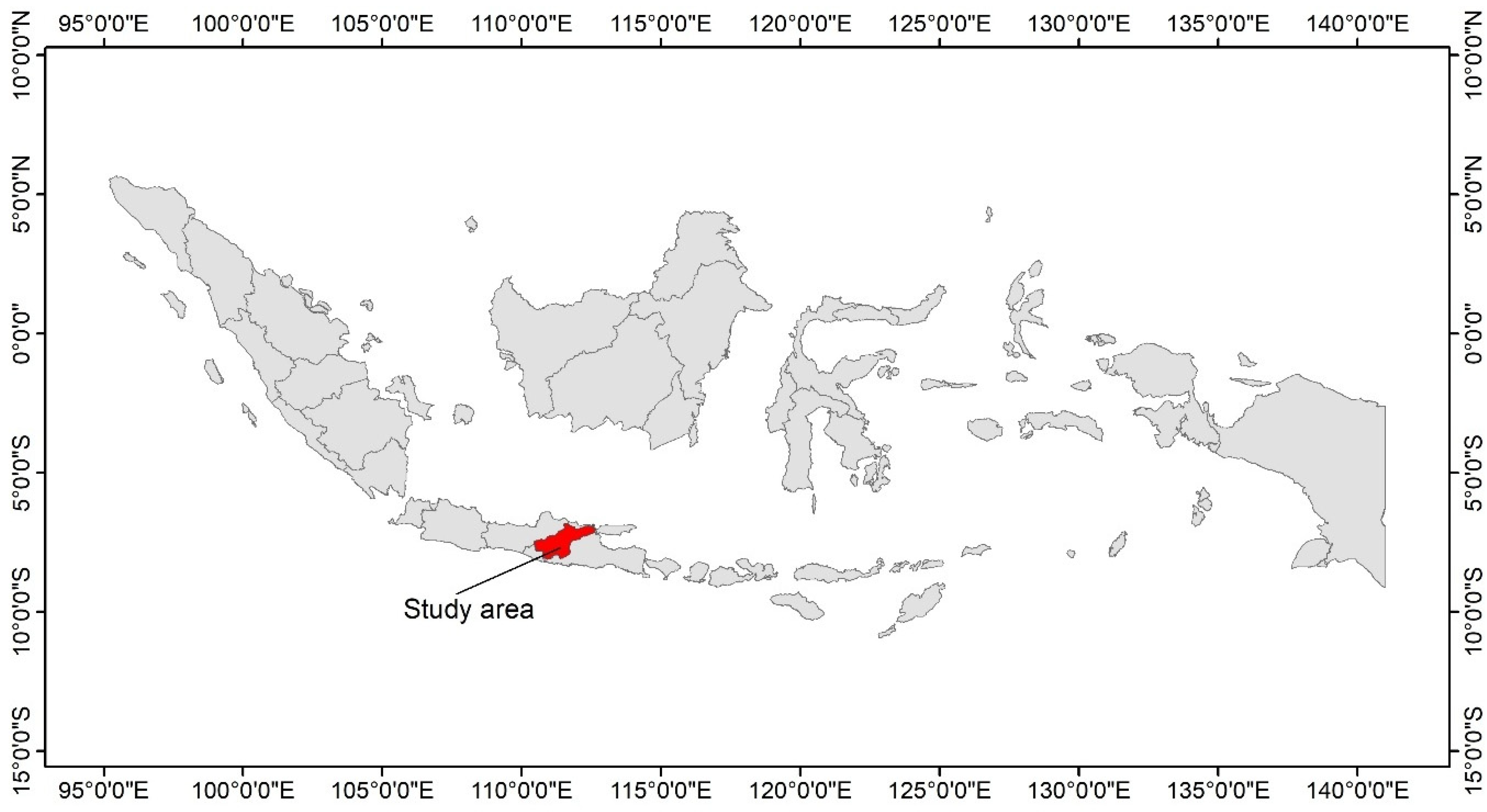
Figure 1. Location of the Bengawan Solo Watershed study area.
Sustainability 17 09281 g001
Figure 2. Research framework.
Sustainability 17 09281 g002
Figure 3. Locations of the sampling points for rainfall data extraction from CHIRPS.
Sustainability 17 09281 g003
Figure 4. Error Metrics of MAE (a), RMSE (b), MAPE (c), and R2 (d) of the Ensemble Predictions.
Sustainability 17 09281 g004
Figure 5. Metric of Correlation Heatmap.
Sustainability 17 09281 g005
Figure 6. R-squared vs. Number of Model Ensembles Plot.
Sustainability 17 09281 g006
Figure 7. Comparison of predicted (P) and real–CHIRSP data (R).
Sustainability 17 09281 g007
Figure 8. Temporal Trend of Average Annual Rainfall from 2025 to 2030.
Sustainability 17 09281 g008
Figure 9. Predicted Spatial Variability of Annual Rainfall (2025–2030) (mm).
Sustainability 17 09281 g009
Figure 10. Error metrics vs. elevation.
Sustainability 17 09281 g010
Table 1. Deep learning parameters.
ModelDropoutLossOptimizerBatchEpochs (max)Early Stop
LSTM0.20HuberAdam 1 × 10−36480patience 10
GRU0.20HuberAdam 1 × 10⁻³, clipnorm = 1.06480patience 10
TCN0.20HuberAdam 1 × 10⁻³, clipnorm = 1.06480patience 10
CNN (1D)0.15 Huber (δ = 1.0)Adam 1 × 10⁻³, clipnorm = 1.064100patience 12
Transformer0.10Huber (δ = 1.0)Adam 1 × 10⁻³, clipnorm = 1.064120patience 12
Table 2. Ensemble Stacking Scenarios for Experiments.
ScenarioBase Models UsedCategory
ARF, XGB, MLP, LGBMBest ML
BRF, XGB, SVR, MLP, LGBMAll ML
CLSTM, GRU, TCN, CNN, TransformerAll DL
DRF, XGB, SVR, MLP, LGBM, LSTM, GRULight ML + DL
ERF, LSTMOne ML + one DL
FRF, XGB, LGBM, LSTM, GRU, TCN, CNN, TransformerSmall ML set + all DL
GRF, XGB, LGBMML minimum (tree ensemble)
HLSTM, GRURecurrent DL only
ICNN, TransformerDL spatial +
JRF, XGB, MLP, LGBM, LSTM, GRU, TCN, CNN, TransformerAll models (exclude SVR)
KRF, MLPSimpler ML
LSVR, LSTMNon-tree ML + DL
MRF, TransformerBest ML + Best DL (hypothetical)
NRF, XGB, SVR, LGBMAll tree + margin-based ML
OGRU, CNN, TransformerNon-LSTM DL
PMLP, LSTM, GRUShallow NN + Recurrent NN
QRF, XGB, SVR, MLP, LGBM, LSTM, GRU, TCN, CNN, TransformerFull stack
Description: RF: Random Forest, XGB: Extreme Gradient Boosting, SVR: Support Vector Regression, MLP: Multi-Layer Perceptron, LGBM: Light Gradient-Boosting Machine, LSTM: Long Short-Term Memory, GRU: Gated Recurrent Unit, TCN: Temporal Convolutional Network, CNN: Convolutional Neural Network, Transformer: Transformer Neural Network.
Table 3. Evaluation of MAE, RMSE, MAPE, and R2 for all base models (ML and DL).
NoModelMAERMSER2MAPE (%)
1RF61.44418884.4236210.6964845.056787
2XGB59.08847680.307870.72535345.903841
3SVR66.85017890.3651390.65225550.787902
4MLP66.49423389.4197530.65949354.942884
5LGBM60.39063984.1545250.69841242.281571
6LSTM66.48011689.5834590.65824548.597533
7GRU59.5924680.7531120.72229951.325625
8TCN76.301859107.7631610.50546262.699634
9CNN83.509829118.27430.40428475.991914
10TRANSFORMER85.433951116.2767540.42423688.148625
Table 4. Ensemble Performance Evaluation Results for Each Scenario (2020–2024 Validation).
ScenarioNumber ofMAERMSEMAPER2
Models
A458.2844574.8993468.615680.761101
B558.2105474.7546868.153320.762023
C554.0306969.9382957.865970.7917
D754.8851670.217560.112310.790034
E258.8957677.2145172.351840.746104
F853.8267669.3326557.991480.795292
G358.368874.9778869.144020.7606
H255.5290171.4883960.781050.782365
I273.7738798.26589108.21560.588789
J953.8212369.3261557.951610.795331
K259.0953977.0805270.577440.746984
L260.2788779.5786472.784440.730318
M258.6872976.9652571.63390.74774
N458.2889574.823668.544380.761584
O356.0562373.9715963.632830.766982
P355.4557171.4063560.370160.782864
Q1053.7341369.1984557.611180.796084
Table 5. Correlation coefficient between error metrics and elevation.
Metricnr (Pearson)ρ (Pearson)r (Spearman)ρ (Spearman)
RMSE5230.6888645118.06 × 10−750.5224415835.77 × 10−38
MAE5230.7157063382.93 × 10−830.5821482059.05 × 10−49
MAPE523−0.2738792341.88 × 10−10−0.46351743.23 × 10−29
R25230.1714056558.16 × 10−50.2290055041.19 × 10−7
Disclaimer/Publisher’s Note: The statements, opinions and data contained in all publications are solely those of the individual author(s) and contributor(s) and not of MDPI and/or the editor(s). MDPI and/or the editor(s) disclaim responsibility for any injury to people or property resulting from any ideas, methods, instructions or products referred to in the content.