Article

Hybrid Wind Power Forecasting for Turbine Clusters: Integrating Spatiotemporal WGANs with Extreme Missing-Data Resilience

School of Automation and Electrical Engineering, Lanzhou Jiaotong University, Lanzhou 730070, China
*
Author to whom correspondence should be addressed.
Sustainability 2025, 17(20), 9200; https://doi.org/10.3390/su17209200
Submission received: 6 August 2025 / Revised: 17 September 2025 / Accepted: 9 October 2025 / Published: 17 October 2025

Abstract

The global pursuit of sustainable development amplifies renewable energy’s strategic importance, positioning wind power as a vital modern grid component. Accurate wind forecasting is essential to counter inherent volatility, enabling robust grid operations, security protocols, and optimization strategies. Such predictive precision directly governs wind energy systems’ stability and sustainability. This research introduces a novel spatio-temporal hybrid model integrating convolutional neural networks (CNN), bidirectional long short-term memory (BiLSTM), and graph convolutional networks (GCN) to extract temporal patterns and meteorological dynamics (wind speed, direction, temperature) across 134 wind turbines. Building upon conventional methods, our architecture captures turbine spatio-temporal correlations while assimilating multivariate meteorological characteristics. Addressing data integrity compromises from equipment failures and extreme weather-which undermine data-driven models-we implement Wasserstein GAN (WGAN) for generative missing-value interpolation. Validation across severe data loss scenarios (30–90% missing values) demonstrates the model’s enhanced predictive capacity. Rigorous benchmarking confirms significant accuracy improvements and reduced forecasting errors.

1. Introduction

Sustainable development has become a global imperative, where energy security fundamentally underpins sustainability agendas worldwide. Projected increases in worldwide energy demand [1] coupled with the inherent constraints of fossil fuel dependence necessitate accelerated renewable energy adoption. Wind power has emerged as a critical renewable alternative, though its inherent variability presents significant grid integration challenges-compromising power quality and system stability during network interconnection [2].
Wind power forecasting addresses these challenges by providing essential data for grid scheduling [3,4] while enhancing system resilience to supply fluctuations [3]. Forecasts are categorized by temporal scale: Ultra-short-term, Short-term, and Medium-to-Long-term [5]. These distinct horizons, respectively, optimize turbine control, power scheduling, and maintenance planning [6].
Methodologically, forecasting techniques comprise four categories: physical, statistical, artificial intelligence (AI), and hybrid approaches. Physical methods, limited in capturing historical wind trends, primarily serve medium-to-long-term forecasts. Statistical approaches excel at extracting historical trends, achieving greater accuracy in both long- and short-term predictions [2]. However, their reliance on linear theory reduces effectiveness against wind power’s stochastic nature.
AI applications in wind forecasting have expanded with technological advancement, including Artificial neural networks, Support vector machines [7], and Long short-term memory networks [8]. These demonstrate superior capability in processing nonlinear relationships and extracting critical temporal information [9].
Most current AI models focus primarily on temporal feature extraction. Yet comprehensive forecasting requires integrating spatial correlations with meteorological feature processing [10]. Wu et al. combined meteorological feature exploration with two-stage decomposition to conduct interpretable wind speed forecasting, achieving excellent results [11]. Furthermore, they pioneered experiments in the multi-dimensional field of feature exploration [12]. This interpretable experimental process and its results have pointed out a new path for decision-makers seeking reliable wind speed forecasting processes and outcomes. Some researchers are also considering adopting decomposition methods for feature collection and prediction [13,14]. Meteorological conditions show consistent patterns across turbines in spatial regions. Leveraging spatial correlations enhances predictions by strengthening data representations and improving model generalization against fluctuations [15]. Therefore, the integration of temporal dynamics, meteorological variables, and spatial dependencies represents a critical research frontier [16].
Recent global research extensively explores spatio-temporal correlations. Ye et al. leveraged spatial correlations between adjacent wind farms to correct wind power prediction outliers, validating the approach with operational data from Northwest China [17]. Zhang et al. designed ST-ResNet as an end-to-end architecture tailored to spatio-temporal data properties, demonstrating convolutional neural networks’ (CNNs) efficacy in extracting spatio-temporal features [18]. Fanhang et al. developed a spatio-temporal neural network combining deep CNNs with bidirectional gated recurrent units. This model extracts spatio-temporal features from historical wind data and numerical weather predictions, achieving high accuracy through feature fusion [19]. Shih et al. confirmed long short-term memory networks’ superiority in multivariate time-series feature extraction [20]. Tba et al. developed a CNN-LSTM framework using Pearson’s correlation coefficients to capture traffic trajectory patterns in graph form [21]. Subsequently, Ja et al. introduced geometric attention-based graph convolutional networks (GCNs) to model dynamic connectivity in traffic flow sensors [22]. However, GCNs show limitations in adapting receptive fields to multi-frequency variables [23].
Maintaining data integrity is crucial for AI-based wind power prediction, going beyond just extracting meteorological, spatial, and temporal features. However, substantial data loss frequently occurs due to unstable communication networks and equipment failures, degrading the accuracy of data-driven models [24]. Solutions for handling missing data primarily encompass three approaches: direct deletion, statistical imputation, and AI-based imputation. Direct deletion removes missing values, but this compromises original data integrity and is only viable when data loss is minimal [25]. Statistical imputation, such as using means or medians, preserves wind farm sequence continuity [26]; however, it overlooks dynamic patterns and introduces systematic bias by treating the data as static. AI imputation methods, like k-Nearest Neighbors (KNN) [27] and Matrix Decomposition [28], generate missing values probabilistically. Despite their sophistication, these methods often fail to effectively model the complex temporal relationships inherent in wind power time-series data.
Consequently, generative adversarial networks (GANs) have gained prominence for data imputation [29]. Yoon et al. developed a GAN-based method employing cue vectors for missing value interpolation [30]. However, GAN-generated data quality depends critically on its objective function. Overly large objectives can trigger vanishing gradients [31]. Thus, Wasserstein distance-based GANs are proposed for generating missing measurements. It is therefore proposed that a Wasserstein distance-based GAN be utilized for the purpose of generating missing measurements [32].
To address these research gaps, we propose a hybrid CNN-BiLSTM-GCN model integrated with Wasserstein GAN (WGAN) for multi-turbine wind power spatiotemporal prediction. Our core contributions are:
  • To capture complex spatiotemporal correlations caused by atmospheric system inertia, we construct a power-enhanced adjacency matrix based on wind turbines’ relative coordinates. Spatial features are extracted via GCN, followed by temporal feature extraction from meteorological and power data using CNN-BiLSTM. This hybrid architecture improves spatiotemporal modeling.
  • WGAN is trained to generate missing data, with optimization guided by mean difference, standard deviation difference, Wasserstein distance, mutual information score, and KL divergence evaluations. This yields an enhanced WGAN generator.
  • Model efficacy was validated with 30–90% missing data simulations. Predictions for 134 turbines across six time steps show superior accuracy and reduced error margins compared to other deep learning models.
Our framework pioneers three key innovations beyond conventional single-task models: it implements a CNN-BiLSTM-GCN hybrid architecture employing power-weighted adjacency matrices for unified spatiotemporal feature extraction; enables simultaneous wind power forecasting for 134 turbines through scalable multi-task learning; and integrates WGAN data restoration to maintain prediction accuracy under extreme 30–90% missing data scenarios-outperforming benchmark methods across validation metrics.
The paper is structured as follows: Section 2 outlines methodologies; Section 3 details technical innovations; Section 4 presents experiments; Section 5 provides discussion and conclusions, along with future prospects.

2. Methods

2.1. Modeling of Spatial and Temporal Correlations

2.1.1. Convolutional Neural Networks

As a specialized deep learning architecture, convolutional neural networks (CNNs) employ convolutional operators to distill high-level temporal patterns and feature correlations within sequential data streams [33]. The one-dimensional convolutional layer enhances accuracy while reducing complexity, demonstrating efficacy in extracting features from noisy data [34].
CNNs provide dual core advantages: efficient localized feature extraction and concurrent parameter reduction. This reduction is achieved through three interconnected mechanisms:
  • Local Receptive Fields (LRF): Neurons connect only to restricted input regions, focusing exclusively on local features;
  • Weight Sharing (WS): Identical filters apply across spatial dimensions, drastically lowering parameters while promoting translational invariance;
  • Pooling: Down sampling operation that:
    (a)
    Retains critical information
    (b)
    Reduces feature map size/computation
    (c)
    Increases model robustness
    (d)
    Mitigates overfitting.
As Figure 1 illustrates, The CNN architecture sequentially processes input data through three functional layers: convolutional layers perform localized feature extraction via filter operations, pooling layers subsequently condense key information through spatial downsampling, and fully connected layers ultimately generate outputs.

2.1.2. Bidirectional Long Short-Term Memory

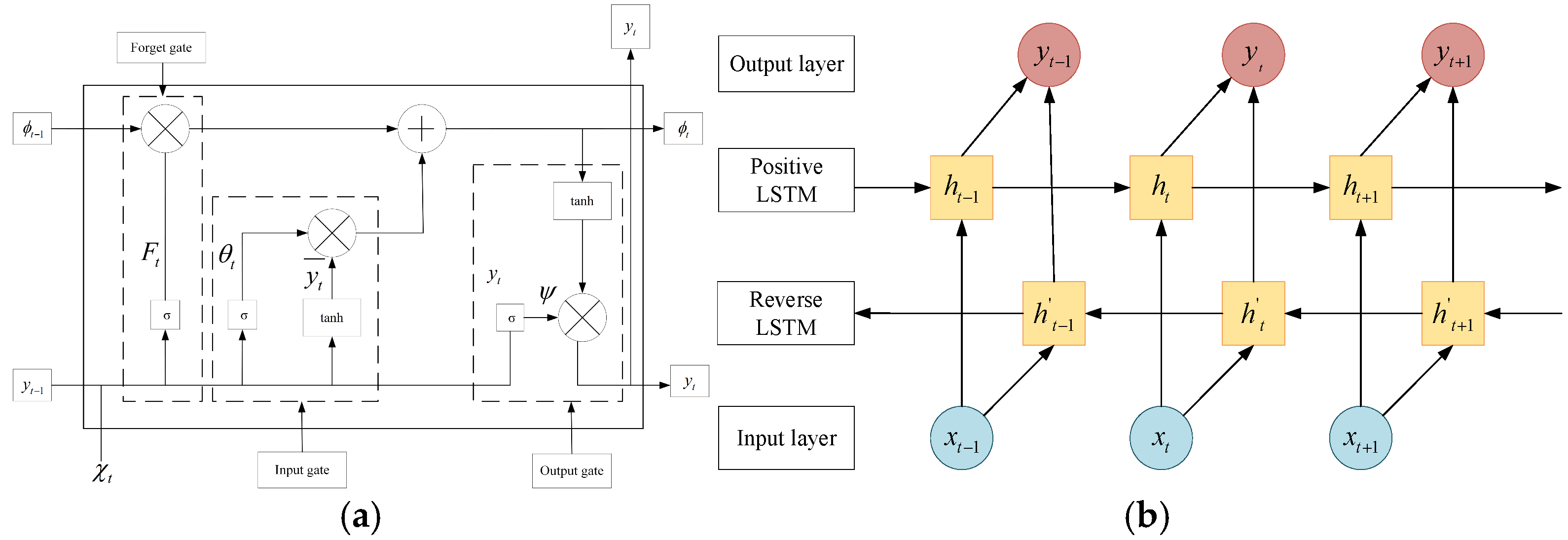
The Long Short-Term Memory (LSTM) network, a specialized recurrent neural network (RNN) variant, was introduced by Hochreiter and Schmidhuber to resolve the gradient vanishing problem inherent in conventional RNNs [35,36,37]. As depicted in Figure 2a, its operational mechanism follows:
F t = σ ( ω f [ y t 1 , χ t ] + a f )
θ t = σ ( ω i [ y t 1 , χ t ] + a i )
ϕ t = tanh ( ω c [ y t 1 , χ t ] + a c )
ϕ t = f t ϕ t 1 + i t ϕ t
ψ t = σ ( ω o [ y t 1 , χ t 1 ] + a o )
y t = ψ t tanh ( ϕ t )
The symbolic parameters F t , θ t , ϕ t , y t and ψ t respectively denote the forget gate activation, input gate state, cell memory vector, post-activation output signal, and temporal output data, while ω f ω o and a f a o represent trainable weight matrices and bias vectors mapped to corresponding operational gates.
Bidirectional Long Short-Term Memory (BiLSTM) networks extend conventional LSTM architectures [38]. As illustrated in Figure 2b, BiLSTM incorporates a backward processing channel that captures additional temporal dependencies. This dual-directional structure enhances extraction of intrinsic patterns from wind power data, significantly improving prediction accuracy.

2.1.3. Graph Convolutional Networks

Graph data exhibit non-Euclidean structures with inherent complexity that traditional neural networks struggle to process. While CNNs effectively handle regular data structures, their spatial invariance and rigid architecture pose limitations for dynamic graph data. These constraints, along with substantial computational demands and data dependency, motivated the development of graph convolutional networks (GCNs) in 2017 [39]. GCNs extend convolutional mapping to graph-structured data, where vertex representations are iteratively refined through localized feature aggregation over node neighborhoods [40].
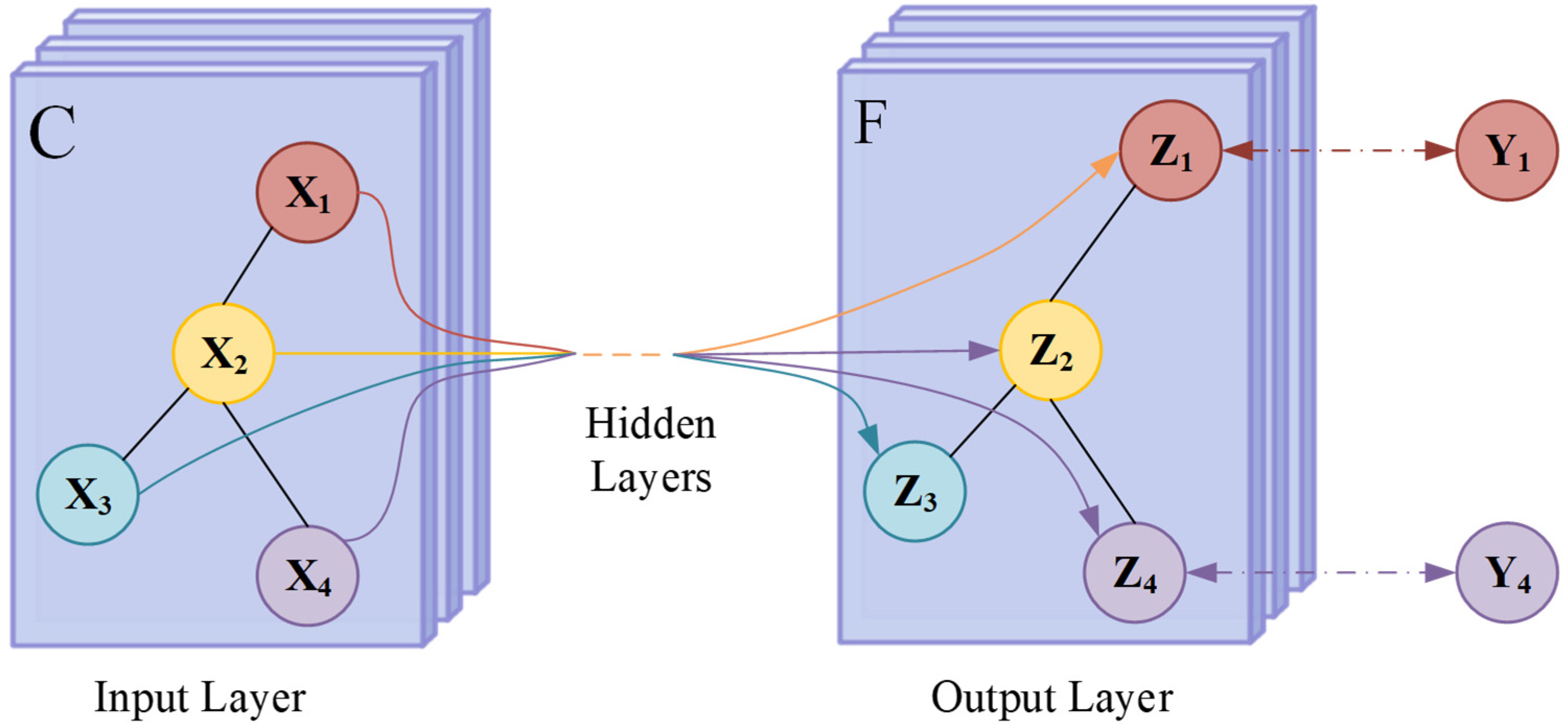
By defining specialized graph convolution operations, GCNs effectively address graph data irregularity and dynamics. The core mechanism relies on the graph convolution operator, Figure 3 shows a schematic diagram of the GCN and defined mathematically as follows:
H ( l + 1 ) = σ ( D ˜ 1 / 2 A ˜ D ˜ 1 / 2 H ( l ) W ( l ) )
where H ( l ) represents the node characterization matrix of layer l . H ( l + 1 ) is the l + 1 th layer output feature matrix. W ( l ) represents the weight matrix of the lth layer. σ denotes the nonlinear activation function. A ˜ is the adjacency matrix after adding the self-connection, and D ˜ is its degree matrix.

2.2. Wasserstein Generating Adversarial Networks

The Wasserstein Generative Adversarial Networks (WGANs), introduced by Arjovsky et al. in 2017, address critical limitations of traditional GANs including training instability, mode collapse, and ambiguous optimization objectives [41,42]. This is achieved through a reformulated loss function that minimizes the Wasserstein distance, which quantifies the minimum “mass transfer” required to transform generated data distributions into real data distributions. As shown in Figure 4, WGAN’s adversarial framework provides smoother gradient signals to the generator, particularly effective when distributions exhibit limited overlap. The Wasserstein distance is formally defined as:
W 1 ( P , Q ) = inf γ Γ ( P , Q ) x y d γ ( x , y )
where P represents the real data distribution; Q represents the production data distribution; and Γ ( P , Q ) is the set of all joint probability distributions that transfer P to Q.
Leveraging the Kantorovich-Rubinstein duality principle, the Wasserstein metric becomes expressible as a trainable objective function in neural networks given discriminator adherence to Lipschitz continuity requirements.
J ( D ) = Ε Z ~ P Z f W ( G ( z ) ) Ε x ~ P γ f W ( x )
WGAN enforces Lipschitz constraints via discriminator weight clipping, enabling effective Wasserstein distance approximation. This approach provides stronger generator gradients that stabilize training dynamics, prevent model collapse, and ensure reliable convergence with smoother learning curves.

3. Framework and Innovations in Research Methodology

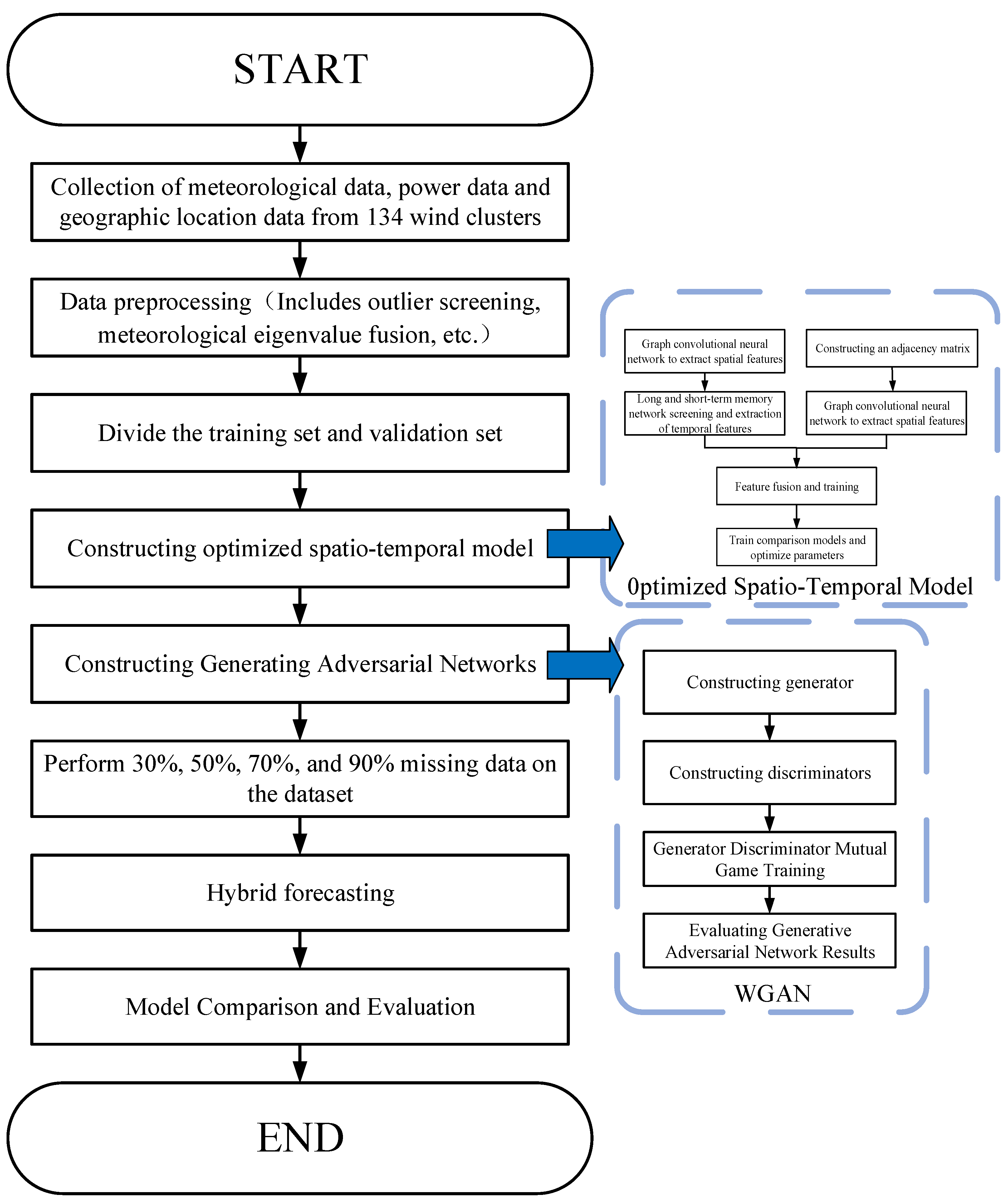
This study integrates an optimized spatio-temporal model-combining convolutional neural networks (CNNs), bidirectional long short-term memory (BiLSTM), and graph convolutional networks (GCNs)-with Wasserstein generative adversarial networks (WGANs) for hybrid prediction. As shown in Figure 5, the methodology proceeds as follows:
  • Data preprocessing: filters operational data from 134 turbines, including power outputs, meteorological variables (wind speed, temperature, direction), and geographic coordinates;
  • Spatio-temporal modeling: employs CNN-BiLSTM for temporal feature extraction and GCN with enhanced power-correlation adjacency matrices for spatial correlation mining. The integrated model is then trained and validated;
  • WGAN training: constructs generators/discriminators optimized through adversarial learning to ensure high-quality data synthesis;
  • Prediction phase: simulates random missing-data scenarios (30%, 50%, 70%, 90%), executing hybrid predictions via the spatio-temporal model and WGAN;
  • Evaluation: benchmarks results against established models using standard metrics.
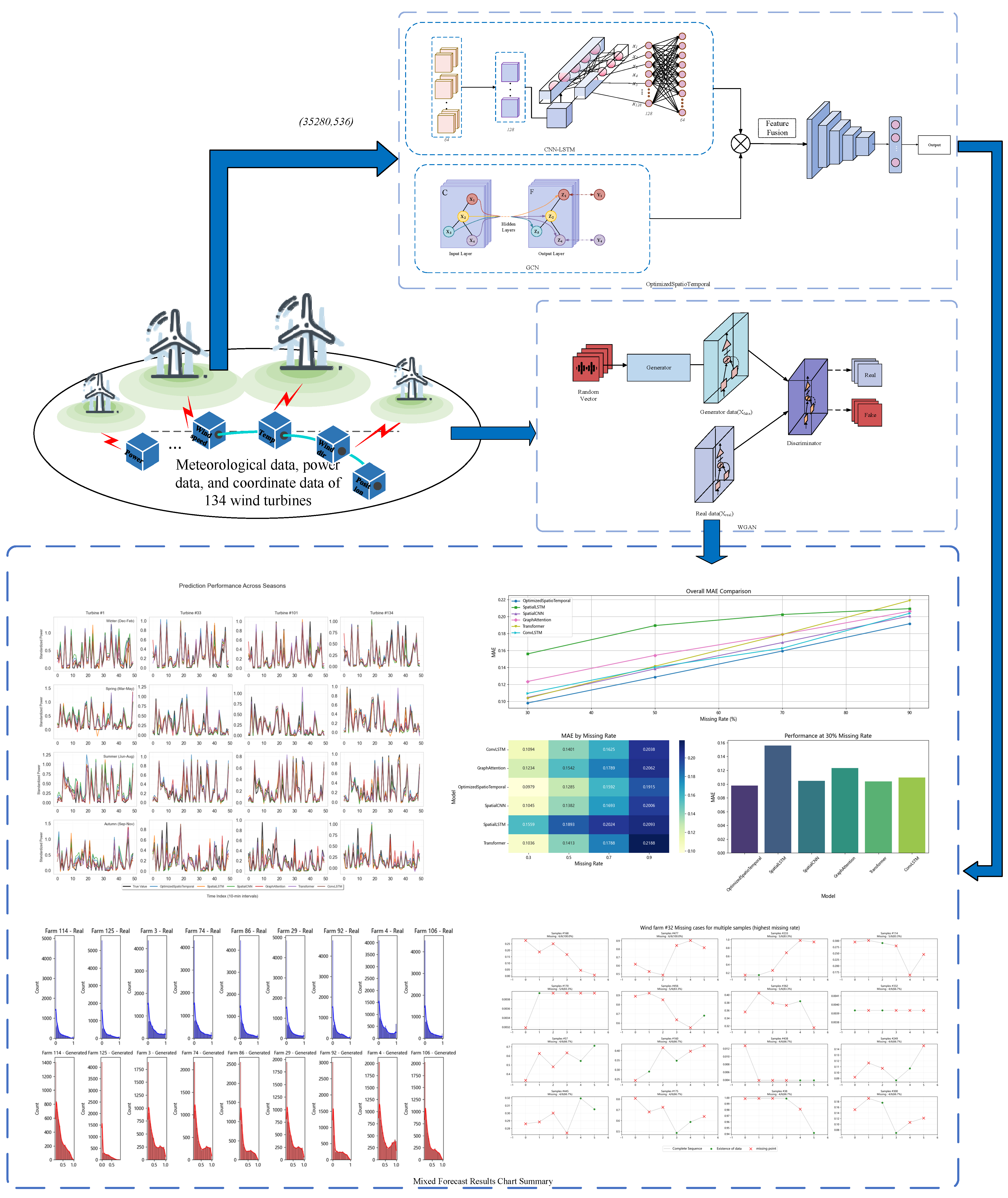
This study introduces a hybrid wind power prediction framework that integrates spatio-temporal correlation analysis with generative adversarial networks (GANs). As illustrated in Figure 6, our core innovations include: first, a unified feature extraction approach where convolutional neural networks (CNNs) combined with bidirectional long short-term memory (BiLSTM) capture multi-scale temporal patterns, while graph convolutional networks (GCNs) derive spatial correlations through power-weighted adjacency matrices; second, scalable forecasting enabling simultaneous power output predictions for all 134 turbines via multi-task learning; and third, robust data gap handling where Wasserstein GANs (WGAN) restore missing measurements during extreme weather events or equipment failures, substantially strengthening model resilience.

4. Experiments and Results

4.1. Data Preprocessing

This study employs Python 3.7 and the Keras framework for model development. The 2022 Baidu KDD Cup dataset from Longyuan Power Group’s SCADA-monitored wind farm provides operational data across 134 turbines, recording 10 min interval power outputs, wind speeds, temperatures, and wind directions over a 245-day period. All turbines comprise standard 1.5 MW land-based units with 0–1500 kW theoretical generation capacity. Actual power outputs exhibit minor inter-turbine variations. Figure 7a shows the spatial relative positions of 134 fans, while Figure 7b presents the correlation analysis between each input variable and power data.
In the analysis of input variables, Pearson’s correlation coefficient is used to measure linear correlation, while mutual information is employed to assess nonlinear correlation. The formulas are as follows:
r = i = 1 n ( x i x ¯ ) ( y i y ¯ ) i = 1 n ( x i x ¯ ) 2 i = 1 n ( y i y ¯ ) 2
I ( X ; Y ) = y Y x X p ( x , y ) log ( p ( x , y ) p ( x ) p ( y ) )
As shown in Figure 7, the 134 wind turbines are located relatively close together. Considering spatiotemporal correlation under these objective geographical conditions is reasonable. Spatiotemporal correlation requires consideration of climatic conditions, with wind speed being the primary climatic factor and wind direction and temperature being secondary factors.
All the input features (including wind power from each turbine, wind speed, temperature, and wind direction) and the target wind power values are normalized into the range [0, 1] using Min-Max normalization. Specifically, for a given feature x , the normalized value x n o r m is calculated as:
x n o r m = x x min x max x min
where x min and x max are the minimum and maximum values of that feature in the training set, respectively.
Four critical features (power, wind speed, temperature, direction) form a 536-dimensional dataset (134 turbines × 4 features). Six-step historical backtracking enables one-hour power prediction for all turbines-a short-term forecasting approach. The dataset splits into 7:3 training-validation sets.
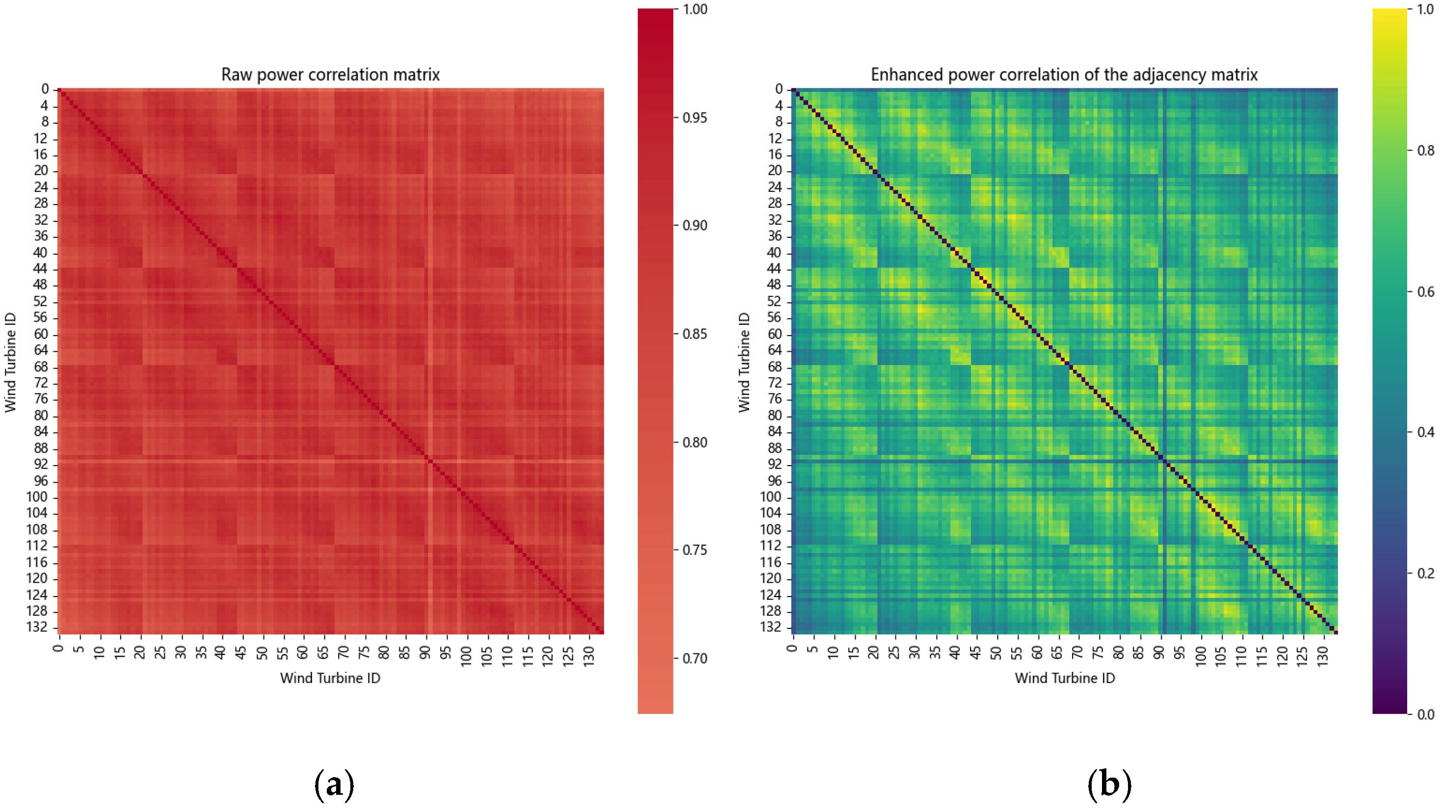
Spatial correlations are captured through power-enhanced adjacency matrices constructed from wind turbines’ geographical relationships. Figure 8 demonstrates how power correlations drive matrix optimization for cluster prediction.

4.2. Spatio-Temporal Model Training and Complete Data Forecasting

The Spatio-temporal Model processes multi-source wind features through a hybrid deep learning architecture. As detailed in Table 1, dual convolutional blocks with 64 and 128 filters sequentially extract localized temporal patterns from the 6-timestep feature window. Bidirectional LSTM layers with 128 and 64 units subsequently capture complex temporal dependencies. Spatial relationships are explicitly modeled using graph-based operations with a correlation-optimized adjacency matrix. Integrated representations are transformed through hierarchical compression layers before generating predictions with linear activation.
In this study, we established five benchmark models: Spatial LSTM, Spatial CNN, Conv LSTM, Transformer, and Graph Attention. All benchmark models and the spatiotemporal model performed prediction experiments on identical datasets. For comparative analysis of prediction results, we employed two statistical validation methods: Paired t-test and Wilcoxon Signed-Rank Test.
The Paired t-test method uses the following formulation:
t = d ¯ μ d 0 s d n
where d ¯ represents the mean difference between paired observations, s d denotes the standard deviation of differences, and n indicates sample size.
The Wilcoxon Signed-Rank Test serves as a nonparametric alternative that does not require normally distributed differences. This method evaluates significance by analyzing signed ranks of differences—considering both the direction (positive/negative sign) and magnitude (absolute rank) of paired differences to construct its test statistic.
Statistical analysis shows p-values below 0.01 for both tests across all model comparisons. These results demonstrate statistically significant performance differences between models.
Following statistical validation, we conducted a multi-faceted evaluation of the spatiotemporal model and benchmark models on the complete dataset. Performance was assessed using Mean Absolute Error (MAE), Root Mean Squared Error (RMSE), and Mean Absolute Percentage Error (MAPE). Robustness was tested by introducing noise and measuring the resultant MAE increase. Model stability was determined through confidence interval analysis. Computational efficiency was evaluated by recording per-epoch training times. The comprehensive evaluation results are presented in Table 2.
M A E = 1 N i = 1 N y i p r e y i
R M S E = 1 N i = 1 N ( y i p r e y i ) 2
M A P E = 1 N i = 1 N y i p r e y i y i p r e × 100 %
where N is the number of samples; y i p r e is the true value; y i is the predicted value. The smaller the value of MAE/RMSE/MAPE, the smaller the error and the better the result.
Figure 9 presents the prediction results of various models under full-data conditions with spatiotemporal correlations. Each subplot displays forecasts for different wind turbines across four distinct seasonal periods. The optimized spatiotemporal model consistently delivers accurate predictions throughout different seasonal intervals. Additionally, within identical time periods, the power output curves of different turbines show strong similarity when exposed to equivalent spatial and climatic conditions.

4.3. Wasserstein Generative Adversarial Network Model Training and Validation

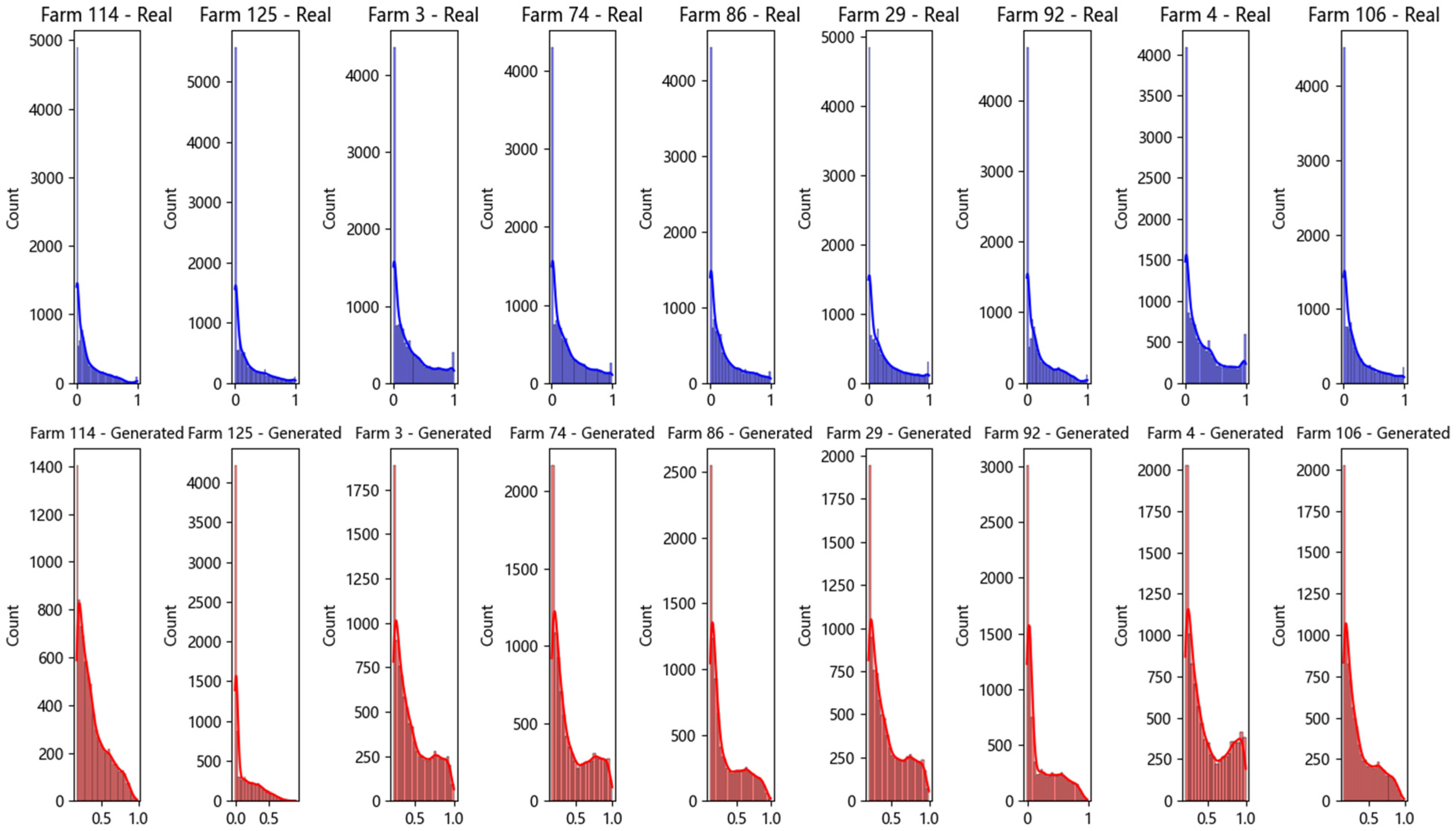
The WGAN training inputs a training set with four features and random noise as generator input. With penalty coefficient set to 15, each iteration involves generator data synthesis and five discriminator updates per round, totaling 200 training rounds. Figure 10 compares generated data against real data distributions.
GAN performance is quantified through four metrics: basic statistics (Equations (11) and (12)), Wasserstein Distance (Equation (8)), Mutual Information Score (Equation (13)), and KL Divergence (Equation (14)). Table 3 quantifies metric outcomes.
M e a n   Difference = 1 d i = 1 d μ r e a l ( i ) μ g e n ( i )
S t a n d a r d   D e v i a t i o n   D i f f e r e n c e = 1 d i = 1 d σ r e a l ( i ) σ g e n ( i )
I ( X ; Y ) = H ( X ) + H ( Y ) H ( X , Y )
D K L ( P Q ) = x P ( x ) log P ( x ) Q ( x )
where d denotes the data dimension; μ r e a l ( i ) and μ g e n ( i ) denote the mean values of the real and generated data in dimension i ; σ r e a l ( i ) and σ g e n ( i ) denote the standard deviation of the real and generated data in dimension i ; H ( X ) is the entropy of x ; H ( X , Y ) is the joint entropy of x and y; P represents the real data distribution; Q represents the production data distribution.

4.4. Hybrid Wind Power Forecasting

This hybrid wind power prediction model simulates multi-turbine forecasting under data loss scenarios caused by power failures or extreme weather. Designed to process 30–90% missing data generated via WGAN, it executes predictions using our spatio-temporal model.

4.4.1. Situation of Missing Data

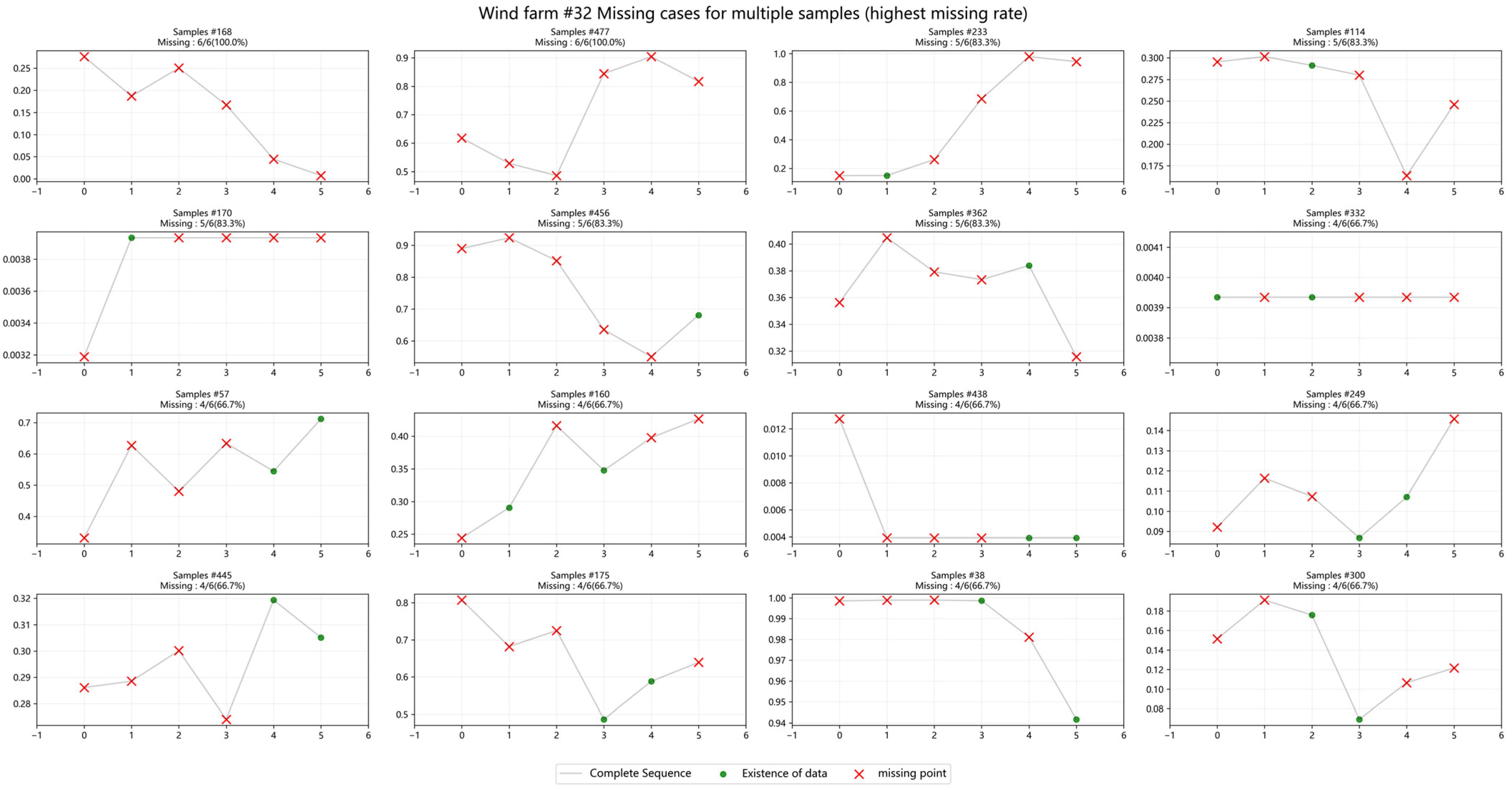
Validation utilizes datasets with randomly missing 30%/50%/70%/90% features. The model incorporates meteorological characteristics including wind speed, temperature, and direction while maintaining the original four-dimensional data structure (134 turbines × 4 parameters). Figure 11 demonstrates Wind Farm 32’s feature reconstruction under 30% missing data.

4.4.2. Hybrid Wind Power Prediction with Different Missing Rates

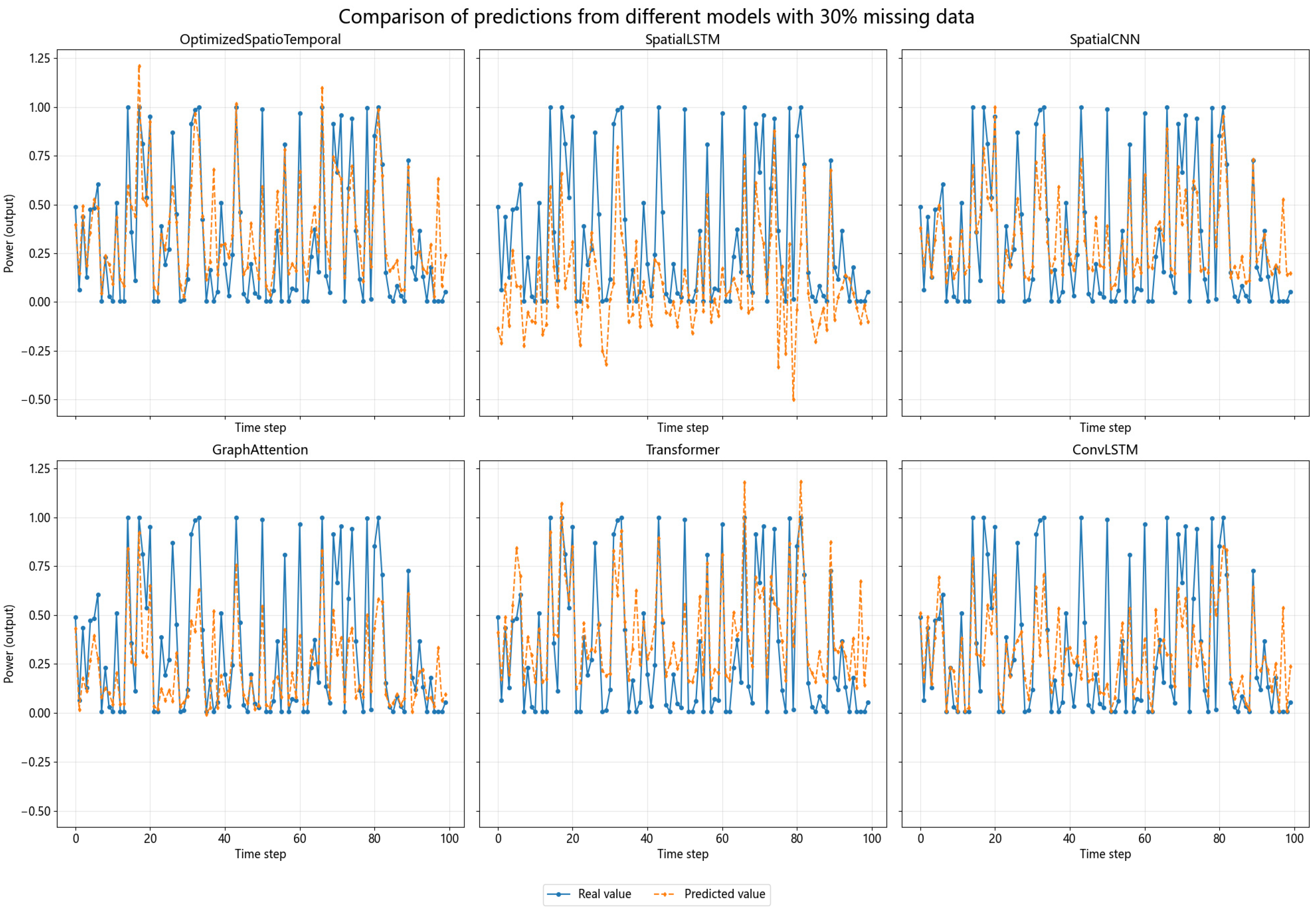
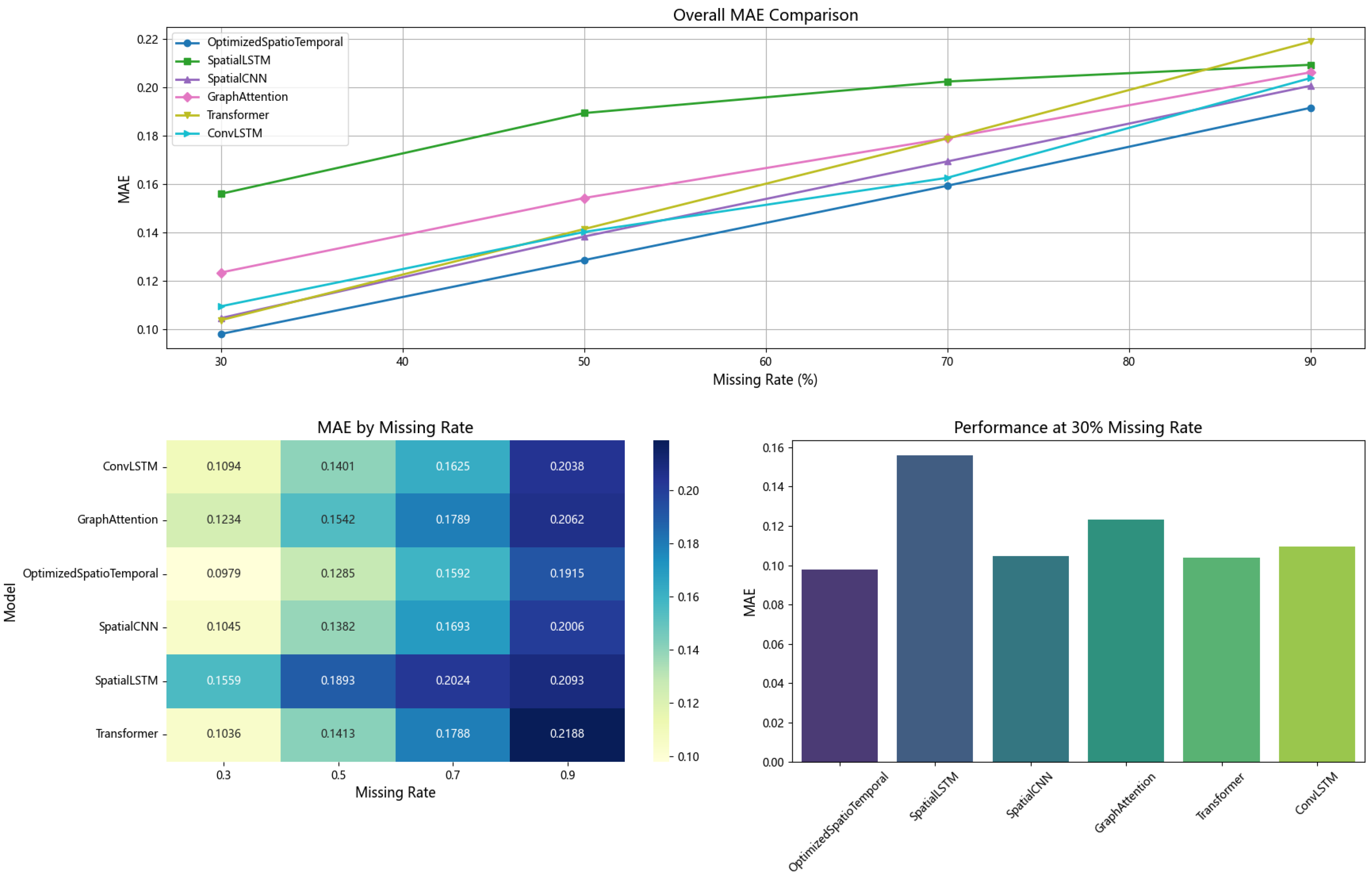
This subsection compares wind power predictions across missing-data scenarios (30–90%). Our hybrid model leverages WGAN to reconstruct missing entries, while benchmark models apply zero-value imputation. Figure 12 contrasts prediction curves at 30% missing data, with comprehensive results synthesized in Figure 13.

5. Discussion of Results and Future Prospects

The subsequent section is dedicated to a detailed discussion and analysis of the results obtained from the experimental study:
  • Spatial Correlation Validation: This study develops a prediction model for 134 wind turbines using 245-day data, integrating meteorological characteristics and spatial correlations. Figure 7 displays turbine positions showing logical spatial distribution. The adjacency matrix effectively strengthens spatial correlations, as evidenced in Figure 9 where actual power curves demonstrate high similarity—confirming significant spatial interdependence. Crucially, Figure 9 also verifies the model’s consistently strong performance across varying seasonal conditions under full data mode.
  • Our spatio-temporal model architecture demonstrates two key advantages. Trained on complete datasets, it integrates convolutional neural networks (CNNs), bidirectional long short-term memory (BiLSTM) networks, and graph convolutional networks (GCNs). This hybrid configuration achieves dual innovations: first, enabling simultaneous power prediction for all 134 wind turbines; second, effectively capturing inter-turbine spatio-temporal correlations. Comparative analysis against five benchmark models (Figure 9 and Table 2) reveals two performance gains: (1) consistent improvements in error metrics, including reduced root mean square error (RMSE), lower mean absolute percentage error (MAPE), and slight mean absolute error (MAE) reductions; (2) enhanced robustness under noisy conditions, evidenced by narrower confidence intervals indicating high prediction consistency. Although architectural complexity increases for feature extraction, computational costs remain manageable while delivering demonstrated predictive advantages.
  • WGAN Data Generation Quality: Using 536 feature dimensions, WGAN-generated data distributions closely match real data. Minimal discrepancies in mean and standard deviation are observed, with Wasserstein distance and KL divergence confirming distributional alignment. Mutual information analysis further verifies retention of meteorological and power data characteristics.
  • Missing Data Robustness: Under 30–90% missing data scenarios, six-step predictions using WGAN imputation outperform alternatives (Figure 11, Figure 12 and Figure 13). While MAE increases with missing data proportion (Figure 12), our hybrid approach maintains high accuracy in the presence of missing data compared to benchmark models.
Compared to conventional wind power forecasting research, this study concentrates on cluster-based forecasting integrating spatio-temporal correlations. Spatial correlations between turbines are captured through an enhanced power correlation-based adjacency matrix, enabling cluster forecasting across 134 turbines. We employ a combined deep learning architecture (CNN-BiLSTM-GCN) for spatio-temporal feature extraction, simultaneously incorporating meteorological features and multi-turbine predictive characteristics. To address data absence from equipment failures or extreme weather, a Wasserstein GAN (WGAN) generates forecasts to fill missing values. Validation covers simulated cases with 30% to 90% missing data, demonstrating the hybrid Spatiotemporal model with WGAN superiority over alternative models in forecast accuracy.
Future work will focus on developing lightweight model deployment solutions, such as edge-computing embedded modules for real-time prediction on individual turbine controllers. We also plan to investigate transfer learning frameworks to adapt validated cluster forecasting models to new wind farms of similar scale, reducing retraining costs. These feasible enhancements leverage existing industrial hardware upgrades, providing cost-effective smart solutions for medium/small wind farms.

Author Contributions

Experimental validation, H.S.; Manuscript writing and algorithm design, Y.D.; methodology, Y.C.; Data analysis, D.L.; validation, W.S. All authors have read and agreed to the published version of the manuscript.

Funding

This research was funded by the Gansu Provincial Outstanding Graduate Student Innovation Star Project, Project No. 2025CXZX-736 and the National Natural Science Foundation of China, No. 52467008.

Institutional Review Board Statement

Not applicable.

Informed Consent Statement

Not applicable.

Data Availability Statement

The original contributions presented in the study are included in the article; further inquiries can be directed to the corresponding author.

Acknowledgments

The authors would like to express their sincere gratitude to the Outstanding Graduate Student Innovation Star Program of the Department of Education of Gansu Province, China, for providing generous support and funding for this study.

Conflicts of Interest

The authors declare no conflicts of interest.

Abbreviations

The following abbreviations are used in this manuscript:
CNNConvolutional Neural Network
Bi-LSTMBidirectional Long Short-Term Memory
GCNGraph Convolutional Network
WGANWasserstein Generative Adversarial Network
GANGenerative Adversarial Network
ST-ResNetSpatio-Temporal Residual Network
KNNk-Nearest Neighbors
MAEMean Absolute Error
KLKullback–Leibler Divergence
EMEarth-Mover Distance
LRFLocal Receptive Field
WSWeight Sharing
SCADASupervisory Control and Data Acquisition

References

  1. Moodley, P. 1—Sustainable Biofuels: Opportunities and Challenges. In Sustainable Biofuels; Ray, R.C., Ed.; Applied Biotechnology Reviews; Academic Press: Cambridge, MA, USA, 2021; pp. 1–20. ISBN 978-0-12-820297-5. [Google Scholar]
  2. Wu, B.; Wang, L. Two-Stage Decomposition and Temporal Fusion Transformers for Interpretable Wind Speed Forecasting. Energy 2024, 288, 129728. [Google Scholar] [CrossRef]
  3. Wang, X.; Li, X.; Su, J. Distribution Drift-Adaptive Short-Term Wind Speed Forecasting. Energy 2023, 273, 127209. [Google Scholar] [CrossRef]
  4. Wang, Y.; Xu, H.; Song, M.; Zhang, F.; Li, Y.; Zhou, S.; Zhang, L. A Convolutional Transformer-Based Truncated Gaussian Density Network with Data Denoising for Wind Speed Forecasting. Appl. Energy 2023, 333, 120601. [Google Scholar] [CrossRef]
  5. Liu, H.; Chen, C. Data Processing Strategies in Wind Energy Forecasting Models and Applications: A Comprehensive Review. Appl. Energy 2019, 249, 392–408. [Google Scholar] [CrossRef]
  6. Zhao, W.; Wei, Y.-M.; Su, Z. One Day Ahead Wind Speed Forecasting: A Resampling-Based Approach. Appl. Energy 2016, 178, 886–901. [Google Scholar] [CrossRef]
  7. Wang, Y.; Wang, D. Wind Power Prediction Based on the Clustered Combination of ARMA and PSO-SVM Methods. In Proceedings of the 2019 IEEE Sustainable Power and Energy Conference (iSPEC), Beijing, China, 21–23 November 2019; pp. 1508–1513. [Google Scholar]
  8. Liu, Y.; Guan, L.; Hou, C.; Han, H.; Liu, Z.; Sun, Y.; Zheng, M. Wind Power Short-Term Prediction Based on LSTM and Discrete Wavelet Transform. Appl. Sci. 2019, 9, 1108. [Google Scholar] [CrossRef]
  9. Wang, Y.; Zou, R.; Liu, F.; Zhang, L.; Liu, Q. A Review of Wind Speed and Wind Power Forecasting with Deep Neural Networks. Appl. Energy 2021, 304, 117766. [Google Scholar] [CrossRef]
  10. Guan, L.; Zhou, B.; Wen, B.; Xu, Q.; Zhan, X.; Wu, L.; Zhuo, Y. Spatiotemporal Correlation Statistic Modeling and Simulation in Multiple Wind Farm Power Sequence. Power Syst. Technol. 2021, 45, 30–39. [Google Scholar] [CrossRef]
  11. Wu, B.; Yu, S.; Peng, L.; Wang, L. Interpretable Wind Speed Forecasting with Meteorological Feature Exploring and Two-Stage Decomposition. Energy 2024, 294, 130782. [Google Scholar] [CrossRef]
  12. Wu, B.; Lin, J.; Liu, R.; Wang, L. A Multi-Dimensional Interpretable Wind Speed Forecasting Model with Two-Stage Feature Exploring. Renew. Energy 2026, 256, 124028. [Google Scholar] [CrossRef]
  13. Zhang, G.; Zhang, Y.; Wang, H.; Liu, D.; Cheng, R.; Yang, D. Short-Term Wind Speed Forecasting Based on Adaptive Secondary Decomposition and Robust Temporal Convolutional Network. Energy 2024, 288, 129618. [Google Scholar] [CrossRef]
  14. Wu, Z.; Xiao, L. A Secondary Decomposition Based Hybrid Structure with Meteorological Analysis for Deterministic and Probabilistic Wind Speed Forecasting. Appl. Soft Comput. 2019, 85, 105799. [Google Scholar] [CrossRef]
  15. Xue, Y.; Chen, N.; Wang, S.; Wen, F.S.; Lin, Z.Z.; Wang, Z. Review on Wind Speed Prediction Based on Spatial Correlation. Autom. Electr. Power Syst. 2017, 40, 161–169. [Google Scholar]
  16. Chen, J.; Zhu, Q.; Shi, D.; Li, Y.; Zhu, L.; Duan, X.; Liu, Y. A Multi-Step Wind Speed Prediction Model for Multiple Sites Leveraging Spatio-Temporal Correlation. Proc. CSEE 2019, 39, 2093–2106. [Google Scholar]
  17. Ye, X.; Lu, Z.; Qiao, Y.; Min, Y.; O’Malley, M. Identification and Correction of Outliers in Wind Farm Time Series Power Data. IEEE Trans. Power Syst. 2016, 31, 4197–4205. [Google Scholar] [CrossRef]
  18. Zhang, J.; Zheng, Y.; Qi, D.; Li, R.; Yi, X.; Li, T. Predicting Citywide Crowd Flows Using Deep Spatio-Temporal Residual Networks. Artif. Intell. 2018, 259, 147–166. [Google Scholar] [CrossRef]
  19. Fan, H.; Zhang, X.; Mei, S.; Yang, Z. Ultra-Short-Term Wind Speed Prediction Model for Wind Farms Based on Spatiotemporal Neural Network. Autom. Electr. Power Syst. 2021, 45, 28–35. [Google Scholar]
  20. Shih, S.-Y.; Sun, F.-K.; Lee, H. Temporal Pattern Attention for Multivariate Time Series Forecasting. Mach Learn 2019, 108, 1421–1441. [Google Scholar] [CrossRef]
  21. Bogaerts, T.; Masegosa, A.D.; Angarita-Zapata, J.S.; Onieva, E.; Hellinckx, P. A Graph CNN-LSTM Neural Network for Short and Long-Term Traffic Forecasting Based on Trajectory Data. Transp. Res. Part C Emerg. Technol. 2020, 112, 62–77. [Google Scholar] [CrossRef]
  22. An, J.; Guo, L.; Liu, W.; Fu, Z.; Ren, P.; Liu, X.; Li, T. IGAGCN: Information Geometry and Attention-Based Spatiotemporal Graph Convolutional Networks for Traffic Flow Prediction. Neural Netw. 2021, 143, 355–367. [Google Scholar] [CrossRef]
  23. Song, Y.; Tang, D.; Yu, J.; Yu, Z.; Li, X. Short-Term Forecasting Based on Graph Convolution Networks and Multiresolution Convolution Neural Networks for Wind Power. IEEE Trans. Ind. Inf. 2023, 19, 1691–1702. [Google Scholar] [CrossRef]
  24. Almeida, R.J.; Kaymak, U.; Sousa, J.M.C. A New Approach to Dealing with Missing Values in Data-Driven Fuzzy Modeling. In Proceedings of the International Conference on Fuzzy Systems, Barcelona, Spain, 18–23 July 2010; pp. 1–7. [Google Scholar]
  25. Silva, L.O.; Zárate, L.E. A Brief Review of the Main Approaches for Treatment of Missing Data. IDA 2014, 18, 1177–1198. [Google Scholar] [CrossRef]
  26. Fang, C.; Wang, C. Time Series Data Imputation: A Survey on Deep Learning Approaches. arXiv 2020, arXiv:2011.11347. [Google Scholar] [CrossRef]
  27. Zhang, S. Nearest Neighbor Selection for Iteratively kNN Imputation. J. Syst. Softw. 2012, 85, 2541–2552. [Google Scholar] [CrossRef]
  28. Luo, X.; Zhou, M.; Leung, H.; Xia, Y.; Zhu, Q.; You, Z.; Li, S. An Incremental-and-Static-Combined Scheme for Matrix-Factorization-Based Collaborative Filtering. IEEE Trans. Automat. Sci. Eng. 2016, 13, 333–343. [Google Scholar] [CrossRef]
  29. Goodfellow, I.; Pouget-Abadie, J.; Mirza, M.; Xu, B.; Warde-Farley, D.; Ozair, S.; Courville, A.; Bengio, Y. Generative Adversarial Networks. Commun. ACM 2020, 63, 139–144. [Google Scholar] [CrossRef]
  30. Yoon, J.; Jordon, J. GAIN: Missing Data Imputation Using Generative Adversarial Nets. In Proceedings of the 35th International Conference on Machine Learning, Stockholm, Sweden, 10–15 July 2018. [Google Scholar]
  31. Zhang, W.; Luo, Y.; Zhang, Y.; Srinivasan, D. SolarGAN: Multivariate Solar Data Imputation Using Generative Adversarial Network. IEEE Trans. Sustain. Energy 2021, 12, 743–746. [Google Scholar] [CrossRef]
  32. Xu, D.; Peng, H.; Wei, C.; Shang, X.; Li, H. Traffic State Data Imputation: An Efficient Generating Method Based on the Graph Aggregator. IEEE Trans. Intell. Transport. Syst. 2022, 23, 13084–13093. [Google Scholar] [CrossRef]
  33. Liao, Z.; Coimbra, C.F.M. Hybrid Solar Irradiance Nowcasting and Forecasting with the SCOPE Method and Convolutional Neural Networks. Renew. Energy 2024, 232, 121055. [Google Scholar] [CrossRef]
  34. Kiranyaz, S.; Avci, O.; Abdeljaber, O.; Ince, T.; Gabbouj, M.; Inman, D.J. 1D Convolutional Neural Networks and Applications: A Survey. Mech. Syst. Signal Process. 2021, 151, 107398. [Google Scholar] [CrossRef]
  35. Hochreiter, S.; Schmidhuber, J. Long Short-Term Memory. Neural Comput. 1997, 9, 1735–1780. [Google Scholar] [CrossRef]
  36. Abdel-Nasser, M.; Mahmoud, K. Accurate Photovoltaic Power Forecasting Models Using Deep LSTM-RNN. Neural Comput. Appl. 2019, 31, 2727–2740. [Google Scholar] [CrossRef]
  37. Shahid, F.; Zameer, A.; Muneeb, M. A Novel Genetic LSTM Model for Wind Power Forecast. Energy 2021, 223, 120069. [Google Scholar] [CrossRef]
  38. Bashir, T.; Wang, H.; Tahir, M.; Zhang, Y. Wind and Solar Power Forecasting Based on Hybrid CNN-ABiLSTM, CNN-Transformer-MLP Models. Renew. Energy 2025, 239, 122055. [Google Scholar] [CrossRef]
  39. Kipf, T.N.; Welling, M. Semi-Supervised Classification with Graph Convolutional Networks. arXiv 2017, arXiv:1609.02907. [Google Scholar] [CrossRef]
  40. Zhou, J.; Cui, G.; Hu, S.; Zhang, Z.; Yang, C.; Liu, Z.; Wang, L.; Li, C.; Sun, M. Graph Neural Networks: A Review of Methods and Applications. AI Open 2020, 1, 57–81. [Google Scholar] [CrossRef]
  41. Arjovsky, M.; Chintala, S.; Bottou, L. Wasserstein Generative Adversarial Networks. In Proceedings of the 34th International Conference on Machine Learning, Sydney, Australia, 6–11 August 2017. [Google Scholar]
  42. Engelmann, J.; Lessmann, S. Conditional Wasserstein GAN-Based Oversampling of Tabular Data for Imbalanced Learning. Expert Syst. Appl. 2021, 174, 114582. [Google Scholar] [CrossRef]
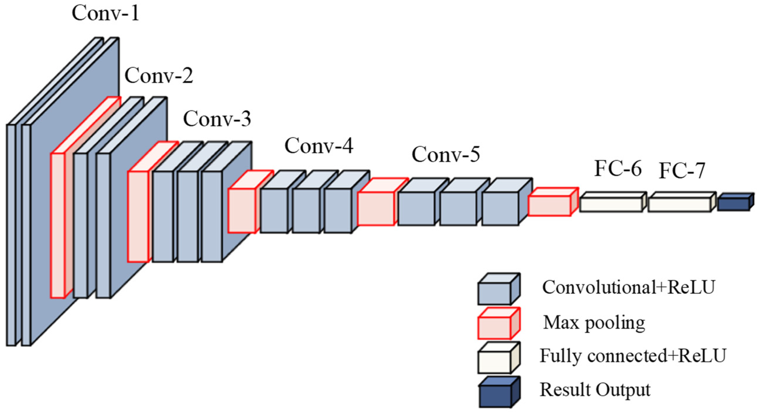
Figure 1. Schematic diagram of CNN.
Sustainability 17 09200 g001
Figure 2. (a) Architectural schematic of LSTM; (b) BiLSTM connectivity topology.
Sustainability 17 09200 g002
Figure 3. Schematic diagram of GCN.
Sustainability 17 09200 g003
Figure 4. Schematic diagram of GAN.
Sustainability 17 09200 g004
Figure 5. Research flowchart.
Sustainability 17 09200 g005
Figure 6. Study schematic.
Sustainability 17 09200 g006
Figure 7. (a) Relative position diagram of wind turbine; (b) Input Variable Importance Analysis Chart.
Sustainability 17 09200 g007
Figure 8. (a) Describes the correlation of raw wind turbines in terms of power; (b) Describes the adjacency matrix after enhanced power correlation.
Sustainability 17 09200 g008
Figure 9. Comparison chart of prediction performance between the Benchmark Model and the model under complete data scenarios across four seasons.
Sustainability 17 09200 g009
Figure 10. Comparison between generated data and real data.
Sustainability 17 09200 g010
Figure 11. WF32 cluster feature reconstruction under 30% data-gap scenario.
Sustainability 17 09200 g011
Figure 12. Multi-model predictive curve alignment at 30% data deletion.
Sustainability 17 09200 g012
Figure 13. Aggregated predictive performance analysis.
Sustainability 17 09200 g013
Table 1. Spatio-temporal model configuration table.
Model ComponentConfigurationPurpose
Input Layer4 features × 6 timestepsFeature-time matrix
Conv1D Blocks64/128 filtersShort-term pattern capture
Bi-LSTM Layers128/64 unitsLong-term dependencies
GCN ModuleAdjacency: Power-correlationSpatial relationships
Dense Layers256/128 unitsFeature fusion
Output LayerLinear activationPower prediction
Table 2. Comprehensive evaluation table of prediction results.
ModelSpatial LSTMSpatial CNNConv LSTMTransformerGraph
Attention
Spatiotemporal
RMSE0.0808240.1035050.1339750.1225500.1146310.078216
MAPE24.97%27.79%34.71%33.69%30.77%20.23%
M A E   1 Original MAE0.0605810.0635270.0874800.0794240.0749030.054105
+5% Noise Robustness8.2%7.5%11.3%9.7%8.9%5.1%
+10% Noise Robustness15.7%14.9%19.8%17.6%16.3%11.8%
+20% Noise Robustness28.4%32.5%33.5%30.2%29.5%24.2%
Statistical Significance 2TrueTrueTrueTrueTrue-
95% CI Lower Bound0.0590.06230.08610.07800.07350.0525
95% CI Upper Bound0.06190.06470.08890.08080.07630.0585
Training Time/Epoch (s)24.322.532.738.941.242.5
1 Percentage change in MAE after input noise; 2 Statistical validation of the comparison between the baseline model and the spatiotemporal model was conducted using the Paired t-test and Wilcoxon Signed-Rank Test methods.
Table 3. Evaluation metrics for evaluating the quality of generative adversarial networks.
Evaluation MetricsValueUnit
Mean Difference0.0720kW
Standard Deviation Difference0.0362kW
Wasserstein Distance0.0574kW
Mutual Information0.7812Bits
KL Divergence0.2450nats
Disclaimer/Publisher’s Note: The statements, opinions and data contained in all publications are solely those of the individual author(s) and contributor(s) and not of MDPI and/or the editor(s). MDPI and/or the editor(s) disclaim responsibility for any injury to people or property resulting from any ideas, methods, instructions or products referred to in the content.