Article

A Three-Stage Super-Efficient SBM-DEA Analysis on Spatial Differentiation of Land Use Carbon Emission and Regional Efficiency in Shanxi Province, China

1
Faculty of Geomatics, Lanzhou Jiaotong University, Lanzhou 730070, China
2
National-Local Joint Engineering Research Center of Technologies and Applications for National Geographic State Monitoring, Lanzhou 730070, China
3
Key Laboratory of Science and Technology in Surveying & Mapping, Lanzhou 730070, China
4
Longnan Normal University, Longnan 742500, China
5
College of Environment and Urban Construction, Lanzhou City University, Lanzhou 730070, China
*
Author to whom correspondence should be addressed.
Sustainability 2025, 17(20), 9086; https://doi.org/10.3390/su17209086 (registering DOI)
Submission received: 8 August 2025 / Revised: 21 September 2025 / Accepted: 22 September 2025 / Published: 14 October 2025
(This article belongs to the Section Sustainability in Geographic Science)

Abstract

Achieving carbon peaking and neutrality is critical for global sustainability efforts and addressing climate change, yet improving land use carbon emission efficiency (LUCE) remains a challenge, especially in resource-dependent regions like Shanxi Province. Existing studies often overlook the spatial heterogeneity of LUCE and the mechanisms behind its driving factors. This study assesses LUCE disparities and explores low-carbon land use pathways in Shanxi to support its sustainable transition. Based on county-level land use data from 1990 to 2022, carbon emissions were estimated, and LUCE was measured using a three-stage super-efficient SBM-DEA model, with stochastic frontier analysis (SFA) to control for external noise. eXtreme Gradient Boosting (XGBoost) with SHAP values was used to identify key socio-economic and environmental drivers. The results show the following: (1) emissions rose 2.46-fold, mainly due to expanding construction land and shrinking cultivated land, with hotspots in Taiyuan, Jinzhong, and Linfen; (2) LUCE improved due to gains in technical and scale efficiency, while pure technical efficiency stayed stable; (3) urbanization and government intervention promoted LUCE, whereas higher per capita GDP constrained it; and (4) population density, economic growth, urbanization, and green technology were the dominant, interacting drivers of land use carbon emissions. This study integrates LUCE assessment with interpretable machine learning, demonstrating a framework that links efficiency evaluation with driver analysis. The findings provide critical insights for formulating regionally adaptive low-carbon land use policies, which are essential for achieving ecological sustainability and supporting the sustainable development of resource-based regions.

.

1. Introduction

Anthropogenic greenhouse gas emissions have been identified as the principal driver of global climate change, posing unprecedented challenges to sustainable development [1]. Among them, carbon emissions are not only the dominant contributor to the greenhouse effect but also a vital indicator for assessing climate impacts [2]. China’s updated Nationally Determined Contributions (NDCs), unveiled at the 75th UN General Assembly, established a phased decarbonization roadmap: achieving carbon peaking by 2030 and carbon neutrality by 2060 through robust policy frameworks [3]. This dual carbon agenda has been institutionalized as a core national strategy under the 14th Five-Year Plan, with detailed implementation mechanisms specified in its energy transition clauses [4]. The 20th CPC National Congress further operationalized this vision through systemic carbon peaking initiatives and a paradigm shift in regulatory focus [5], transitioning from dual energy consumption controls to a dual carbon governance system [6].
The IPCC Special Report on Climate Change and Land (SRCCL) identifies terrestrial ecosystems as pivotal climate regulators and reveals that 23% of global greenhouse gas emissions originate from agricultural production, forestry operations, and land use practices [7]. Simultaneously, natural terrestrial carbon sinks currently absorb atmospheric CO2. volumes equivalent to 33% of annual industrial and fossil fuel emissions. This dual functionality makes sustainable land management a key climate mitigation tool and an essential part of carbon neutrality goals in China [8]. Recent studies demonstrate that systematic optimization of land use configurations, particularly through spatial planning innovations combined with energy mix transitions and industrial structure modernization, constitutes a primary driver for unlocking emission reduction capacities [9,10]. Such integrated approaches have consequently emerged as focal points in global climate governance discourse, recognized as foundational methodologies for accelerating decarbonization processes.
Accelerated urbanization and industrial expansion have driven construction land growth beyond regional ecological thresholds in multiple areas [11], significantly compromising localized environmental rehabilitation efforts aimed at achieving ecological equilibrium [12]. To address this challenge, Shanxi provincial authorities implemented the Ecological Province Construction Plan (2021–2030) in 2022. This policy framework integrates three core mechanisms: (1) systematic optimization of territorial spatial configurations, (2) strategic upgrading of industrial structures, and (3) phased transition of energy infrastructure, all guided by ecological civilization principles. This context underscores the urgent need for empirical analysis of land use-related carbon emission dynamics and their driving factors in Shanxi Province. Such research holds immediate relevance for the region’s sustainable transition while advancing theoretical foundations for low-carbon spatial governance [13].
IPCC assessments and empirical studies consistently demonstrate that land use alterations significantly influence carbon cycle dynamics [14,15]. Poorly structured land systems destabilize ecosystem carbon source–sink equilibrium through diminished soil carbon stocks and weakened vegetation sequestration efficiency [16,17]. Recent LUCE research advances span five domains: emission quantification methodologies [18,19], spatiotemporal evolution analysis [20], driver factors identification [21], carbon sink modeling [22,23], and sustainable land management frameworks [24]. Liu et al. [25] further establish that ecosystem carbon emission responses to land use transitions are contingent on synergistic interactions between environmental variables and land use pattern dynamics. These findings necessitate high-resolution, long-term, and national-scale mapping of land use change typologies to ensure accurate carbon accounting.
Researchers widely use nonparametric methods like DEA to assess LUCE [26,27]. Conventional DEA models, however, neglect key parameters such as radial direction and angle selection. This oversight causes measurement inaccuracies due to slack variable limitations. The SBM model with undesirable outputs addresses these flaws, enhancing accuracy in estimating total factor productivity (TFP) for LUCE studies [28]. The super-efficiency SBM-DEA further improves discrimination among efficient decision-making units. Despite these improvements, traditional DEA and SBM models still struggle to incorporate stochastic errors and environmental heterogeneity, leading to mismatches between theoretical models and empirical data [29]. The three-stage DEA framework developed by Fried [30] resolves this by isolating external environmental factors and random disturbances. For example, Yang et al. [31] applied this framework in the Yangtze River Economic Belt, achieving precise LUCE evaluations. These methodological innovations establish a theoretical foundation for implementing the three-stage SBM-DEA model in this study.
This study advances land use carbon emission analysis by integrating a three-stage super-efficient SBM-DEA model and interpretable machine learning techniques (XGBoost and SHAP) at the prefecture level. The SBM-DEA model enhances LUCE evaluation by addressing environmental heterogeneity and stochastic noise, overcoming limitations of conventional efficiency assessments. Meanwhile, machine learning identifies key socio-economic and environmental drivers of carbon emissions and reveals their complex nonlinear interactions. Focusing on Shanxi Province, a resource-dependent region experiencing rapid land use change, this integrated framework provides novel, spatially explicit insights to support regionally adaptive low-carbon land use policies aligned with regional dual carbon goals.

2. Methods

2.1. Study Area

Shanxi Province, located on the eastern Loess Plateau of China, covers 156,700 km2, with terrain dominated by mountains and hills. Elevation gradually decreases from northeast to southwest. As of 2023, the province had a permanent population of 34.66 million and a regional GDP of RMB 2.57 trillion. Characterized by a temperate continental monsoon climate, Shanxi experiences an average annual temperature of 10.7 °C and receives 479.5 mm of precipitation. A major coal producer with over 120 commercially exploited mineral resources, Shanxi has faced significant decarbonization challenges since becoming a national carbon-peaking pilot province in 2023. These geographic and economic conditions intensify land use carbon emissions, creating critical obstacles to achieving regional and national climate targets. Consequently, analyzing land use carbon dynamics in this region holds urgent scientific and policy relevance. The study area is shown in Figure 1.

2.2. Data

The study utilized multi-source geospatial and socio-economic datasets. Land use data spanning 1990–2022 with 30 m spatial resolution was obtained from the Wuhan University Geospatial Dataset (https://zenodo.org). Vegetation dynamics were characterized using 1 km-resolution NDVI data from the Resource and Environmental Science Data Center (https://resdc.cn). Municipal statistical yearbooks provided urbanization rates and GDP metrics, while climate variables (temperature/precipitation) were acquired from the National Earth System Science Data Center (https://www.geodata.cn). Green technology innovation indicators were derived from patent records curated by the Chinese National Intellectual Property Administration (https://www.cnipa.gov.cn).

2.3. Research Methodology

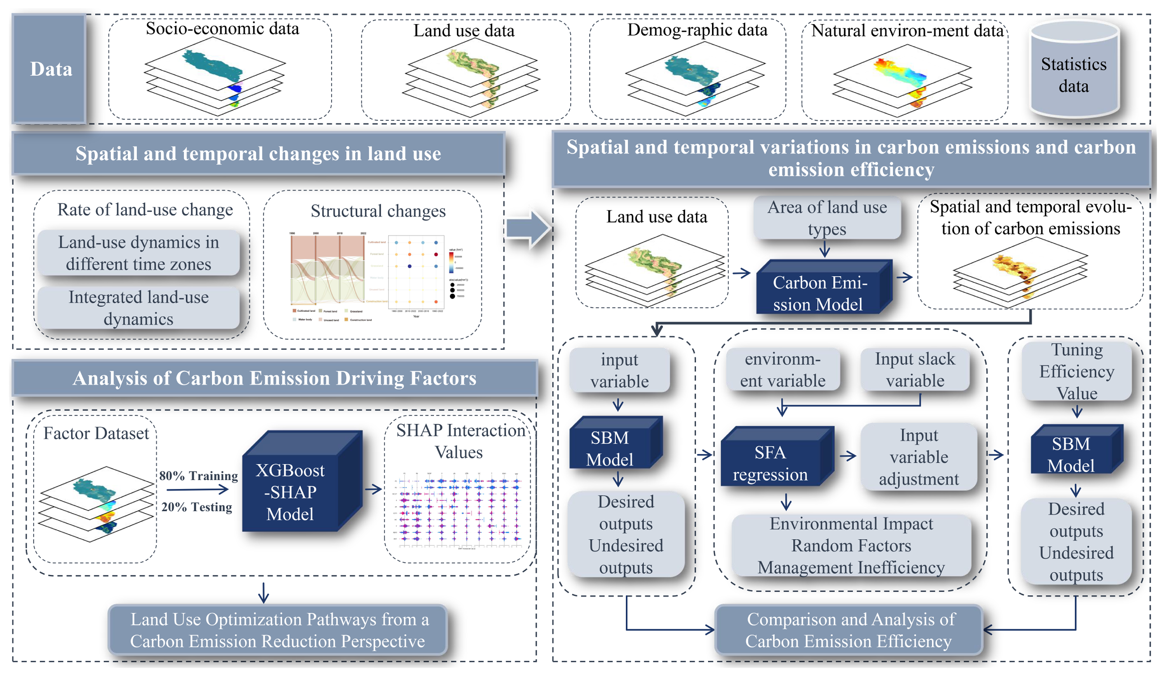
This study pursues two primary objectives: systematically quantifying land use carbon emissions across all 117 county-level administrative units in Shanxi Province, and evaluating land use carbon emission efficiency (LUCE) through efficiency metrics. Based on the empirical results, region-specific mitigation strategies are proposed to support sustainable land governance. The integrated methodological framework, comprising data processing, efficiency evaluation, and policy recommendation modules, is presented in Figure 2.

2.3.1. Dynamic Changes in Land Use Types

Land use dynamics are driven by multiple factors, such as regional economic development, population growth, policy shifts, and environmental changes. These dynamics are typically quantified by assessing the net changes across different land use categories. The dynamic degree of a specific land use type is primarily reflected by its area change during the study period and is calculated using the following formula:
Y c = W b W a W a × 1 T × 100 %
L C = i = 1 n Δ L U i 2 i = 1 n L U i × 1 T × 100 %
where Y c represents the dynamic degree of a specific land use type; W a denotes the initial area of the land use type; W b indicates its terminal area; T signifies the study period duration; L C corresponds to the comprehensive dynamic degree of land use types; L U i refers to the initial area of the i-th land use category, and Δ L U i designates the total area converted from land use type i to non-i categories during the study period.
Land use transition matrices systematically quantify inter-category conversions through time-series comparisons, with the formal calculation shown in Equation (3):
l i j = l 11 l 12 l 1 n l 21 l 22 l 2 n l n 1 l n 2 l n n
where l i j represents the total area converted from category i to category j during a specified period, and n denotes the total number of land use categories.

2.3.2. Estimation of Land Use Carbon Emissions

Shanxi Province comprises 117 county-level administrative units, where long-term, high-resolution energy and agricultural statistics at the county scale are limited. Therefore, we employed the widely used emission-coefficient (emission-factor) approach to estimate land use carbon sources and sinks. Baseline land-type emission coefficients were taken from established national studies [33] and then locally recalibrated to reflect Shanxi’s specific socio-ecological and management conditions, following the regional adaptation methodology demonstrated in Yuan et al. [34].
This recalibration was based on province-specific parameters and their ratios to national averages. For construction land, our recalibrated energy consumption parameter and the resulting high-emission coefficient are consistent in magnitude with the provincial-scale building carbon emission (BCE) intensities recently reported for China by Xie et al. [35], lending strong external validity to our estimate. The complete calibration scheme, including the specific parameters used, the calculated adjustment factors, and the resulting magnitude of adjustment for each land use type, is systematically presented in Table 1.
This hybrid approach—combining baseline factors with province-level recalibration—has been widely applied in regional LUCC studies to reduce bias introduced by spatial heterogeneity [36]. The tabular presentation of the calibration process ensures full transparency and reproducibility of our methodology. Accurate determination of these category-specific emission factors forms the critical methodological foundation for this analysis. This approach has also been commonly employed in studies of similar inland regions, where water bodies were excluded or maintained consistent with baseline values due to data limitations and their comparatively minor role in terrestrial carbon dynamics. For instance, Zhang et al. [37] excluded water bodies when assessing carbon balance changes in terrestrial ecosystems of the Southern United States. Similarly, Tang et al. [38] focused on major vegetated land types (forests, shrublands, grasslands, and cultivated) in compiling China’s terrestrial carbon pools, while giving less emphasis to wetlands and water areas. Therefore, in this study, no recalibration was applied to water bodies.
Cultivated land acts as both a carbon source and sink. Emissions arise from soil organic decomposition, fertilizer use, and crop residue management, while carbon sinks occur via biomass growth and soil carbon storage. Forests and grasslands function primarily as net carbon sinks due to continuous CO2 absorption and vegetation–soil carbon retention. Water bodies show variable carbon cycling, classified here as carbon sinks following established regional studies and IPCC guidelines [39]. Unused land serves as a stable sink with minimal emissions. Construction land remains a dominant carbon source from energy-intensive development. This study categorizes high-emission types (construction and cultivated land) as sources and sequestering ecosystems (forest, grassland, water bodies, and unused land) as sinks within the analytical framework, in line with classifications widely adopted in regional land carbon assessments [35,40].
To ensure analytical consistency, the final recalibrated carbon emission coefficients applied in this study are summarized in Table 2. In this framework, positive values represent carbon emissions, while negative values indicate carbon sinks.
Based on these parameters, a carbon emission estimation model was constructed to evaluate land use patterns in Shanxi Province:
E i = V i × L i , i = 1 , 2 , , 6
where E i represents the carbon emissions (or absorption) generated by the i-th land use type; V i denotes the recalibrated carbon emission coefficient for the i-th land use type; and L i corresponds to the area of the i-th land use type.

2.4. Spatial Autocorrelation Analysis

To assess the spatial clustering patterns of the estimated carbon storage, this research employed spatial autocorrelation analysis. The global Moran’s Index was applied to evaluate the overall degree of spatial aggregation or dispersion, as described by Equation (5). Subsequently, the local Moran’s Index was used to identify specific locations of significant clusters or spatial outliers, as shown in Equation (6).
I = n S 0 × i = 1 n j = 1 n w i j ( y i y ¯ ) ( y j y ¯ ) i = 1 n ( y i y ¯ ) 2
where I represents the global Moran’s Index, with values spanning the interval [ 1 , 1 ] . Values trending toward 1 indicate positive spatial autocorrelation, whereas values approaching 1 signify negative spatial autocorrelation. Values approximating 0 reflect a random spatial distribution.
I i = ( y i y ¯ ) S 2 j = 1 n w i j ( y j y ¯ )
where I i represents the local Moran’s Index for a specific area i. The variance of carbon storage across areas is denoted by S 2 . y ¯ represents the mean carbon storage across all areas; y i and y j represent the carbon storage of area i and j; w i j denotes the spatial weighting coefficient between areas i and j.

2.4.1. Estimation of Land Use Carbon Emissions Efficiency

The three-stage DEA model is widely applied to assess carbon emission efficiency by isolating environmental heterogeneity, yet conventional methods frequently overlook undesirable outputs like carbon emissions. To bridge this gap, a non-radial, non-oriented three-stage DEA framework integrating undesirable outputs is introduced. This framework employs slack variables to quantify inefficiencies (e.g., input redundancies and excessive emissions), enabling targeted efficiency adjustments. Super-efficiency decomposition further enhances discrimination among efficient DMUs while controlling external environmental factors, thereby improving the accuracy of LUCE efficiency evaluations. To achieve this objective and to ensure the comparability of efficiency scores over the long-term study period, a global reference set was adopted by pooling all DMUs from all four years (1990, 2000, 2010, and 2022) to construct a single meta-frontier. This approach provides a constant benchmark against which the temporal evolution of efficiency can be accurately measured.
  • Stage 1: Preliminary calculation of carbon emission efficiency values
    For 11 cities (1990–2022) in Shanxi Province, the conventional DEA is replaced with a super-efficiency SBM model to better align with regional characteristics. Unlike radial DEA approaches that require proportional input-output adjustments, the SBM framework directly optimizes slack variables to quantify resource inefficiencies. The mathematical formulation of Stage 1 is detailed below:
    min 1 1 m i = 1 m s i x i k 1 + 1 S 1 + S 2 r = 1 S 1 s r g y r k g + r = 1 S 2 s r b y r k b s . t . x j = X λ + s y j g = Y g λ s g y j b = Y b λ + s b s 0 , s g 0 , s b 0 , λ 0
    Here, s R m and s b R S 2 denote the input slack variables and the undesirable output slack variables, respectively, while s g R S 1 represents the undesirable output shortfall variables. The parameters m, S 1 , and S 2 denote the number of input variables, desirable output variables, and undesirable output variables, respectively. For the j-th decision-making unit (DMU), ( x j , y j g , y j b ) correspond to its input vector, desirable output vector, and undesirable output vector, respectively, while ( X , Y g , Y b ) represent the aggregate input, desirable output, and undesirable output values across all DMUs. Assuming there are m DMUs, λ R m indicates the weight coefficients for efficiency computation.
    Due to the nonlinear complexity of Equation (7), it is reformulated into an equivalent linear programming problem using mathematical manipulation. The linearized form is mathematically expressed as follows:
    min t 1 m i = 1 m S i x i k s . t . 1 = t + 1 s 1 + s 2 r = 1 s 1 s r g y r k g + r = 1 s 2 s r b y r k b x i t = X Λ + S y k g t = Y g Λ S g y k b t = Y b Λ + S b S 0 , S g 0 , S b 0 , Λ 0 , t > 0
    Let ( λ * , s * , s g * , s b * ) and ( Λ * , t * , s * , s g * * , s b * * ) denote the solutions to Equations (7) and (8), respectively. These solutions satisfy the following relationships, as shown in Equation (9).
    λ * = Λ * / t * , s * = s * / t * , s g * = s g * / t * , s b * = s b * / t *
    By solving Equation (8), the solution to Equation (7) can be derived directly.
  • Stage 2: Adjustment of input variables
    The super-efficiency SBM model is applied in the first stage to quantify input slack variables, but it produces efficiency estimates influenced by environmental heterogeneity and statistical noise. To address this methodological constraint, an SFA framework following Fried et al. (2002) was implemented using Frontier 4.1 software [30]. This approach statistically decomposes observed slack variables into three components: environmental factors, stochastic disturbances, and managerial inefficiencies. The decomposition enables precise identification of dominant environmental and stochastic influences. The SFA regression structure is mathematically defined as follows:
    s i j = f ( Z j ; β i ) + v i j + μ i j ( i = 1 , 2 , , I ; j = 1 , 2 , , J )
    Here, s i j denotes the slack variable of the i-th input for the j-th DMU; Z j represents the vector of environmental variables; β is the vector of coefficients to be estimated; f ( Z j ) captures the influence of environmental variables on the slack variable s i j , typically specified as a linear functional form. v i j captures stochastic noise, assumed to follow a normal distribution with a mean of 0 and variance of σ v 2 , i.e., v i j N ( 0 , σ v 2 ) ; and μ i j reflects management inefficiency, assumed to follow a half-normal distribution μ i j N + ( 0 , σ μ 2 ) . The composite error term v i j + μ i j assumes independence between v j and μ j , with no cross-correlation.
    Environmental factors, stochastic noise, and managerial inefficiency were disentangled. Managerial inefficiency was isolated using the conditional decomposition method proposed by Luo et al. (2012) [41]:
    E ( μ | ε ) = σ * × Φ λ ε σ + λ ε σ ψ λ ε σ
    where
    σ * = σ μ σ v σ , σ = σ μ 2 + σ v 2 , λ = σ μ σ v , ε = v i j + μ i j , γ = σ μ 2 σ μ 2 + σ v 2
    σ μ and σ v denote the standard deviations of management inefficiency and stochastic noise, respectively; Φ and ψ represent the probability density function and cumulative distribution function of the standard normal distribution.
    Using Equation (11), the mixed error and random disturbance terms can be separated as follows:
    E ( v i j | ν i j + μ i j ) = S i j f ( Z j ; β i ) E ( μ i j | v i j + μ i j )
    An SFA regression model was developed to eliminate environmental factors and stochastic noise in efficiency evaluation, ensuring that all DMUs operate under identical external conditions.
    Input variables were subsequently adjusted using Equation (13) after removing environmental and random effects through Equation (12):
    x i j * = x i j + max f ( Z j ; β i ) f ( Z j ; β i ) + max ( v i j ) v i j
    Here, x i j * denotes the adjusted input, and x i j represents the original input. The adjustment has two components:
    Environmental equalization: max f ( Z j ; β i ) f ( Z j ; β i ) neutralizes disparities caused by environmental heterogeneity, homogenizing external conditions across DMUs.
    Stochastic noise normalization: max ( v i j ) v i j calibrates inputs by penalizing DMUs disproportionately affected by stochastic noise (increasing inputs for units with large stochastic noise; decreasing them otherwise).
    This dual adjustment ensures DMUs operate under environmental and stochastic noise baselines, enabling fair efficiency comparisons.
  • Stage 3: Calculate the adjusted efficiency values
    The adjusted efficiency values were measured using the super-efficiency SBM model. This process removed environmental factors and random disturbances from DMU efficiency assessments. The results reflect more authentic, effective efficiency under homogeneous conditions. This adjustment ensures that the efficiency values are determined solely by internal technological and managerial factors, enabling a fairer comparison of actual efficiency across DMUs.
  • Robustness checks
    To ensure the credibility of our findings, we conducted multiple robustness checks addressing key methodological concerns and parameter uncertainties.
    Water-body-neutral scenario: To test the core assumption of water bodies as a carbon sink—a primary source of uncertainty—a conservative sensitivity analysis was conducted by setting their net carbon flux to zero ( V water = 0 ). All other procedures (Section 2.3.2 and Section 2.4.1) remained unchanged. The high consistency in city efficiency rankings between this and the baseline scenario (Spearman’s ρ > 0.8 , p < 0.01 ; see Results Section 3.4.5) confirms the robustness of the comparative conclusions. A neutrality scenario for water bodies is reported in the Results section and detailed in Appendix A.
    Model specification checks: To account for potential spatial dependence in the second-stage SFA residuals, we employed a Spatial Error Model (SEM). The spatial weights matrix W was constructed based on the Queen contiguity criterion, whereby two geographical units are defined as neighbors if they share either a border or a vertex. A first-order contiguity matrix was adopted, considering only direct neighbors. The binary adjacency matrix ( w i j = 1 if i and j are neighbors; 0 otherwise) was row-standardized so that each row sums to unity, ensuring comparability across units. The SEM was then specified as
    u = λ W u + ε ,
    where u denotes the inefficiency residuals, λ the spatial autocorrelation coefficient, and ε the i.i.d. error term. An insignificant λ indicates negligible bias from spatial autocorrelation.
    Monte Carlo uncertainty analysis: To propagate uncertainty in land use emission coefficients (Table 1), we performed a 1000-iteration simulation. Coefficients were perturbed by ± 30 % ( C i , i t e r U ( 0.7 × C i , b a s e , 1.3 × C i , b a s e ) ), and the entire analytical pipeline (Equation (4) AND SBM-DEA model) was rerun per iteration to quantify uncertainty in final efficiency scores.
  • Selection of carbon emission efficiency evaluation indicators
    The carbon emission efficiency evaluation system in this study is constructed based on a classical economic production framework to ensure scientific validity, consistency, and regional applicability. In this framework, three canonical factors of production—capital, labor, and land—are specified as inputs [42]. Specifically, land use categories directly participate in the socio-ecological production process: construction and cultivated land are essential for economic output, while forest and grassland directly contribute to carbon emissions and sinks. Environmental variables (e.g., urbanization rate and industrial structure) influence production efficiency but are not themselves consumed or transformed [30]. This classification aligns with established research on LUCE [43,44,45].
    DMUs and time horizon: The 11 prefecture-level cities in Shanxi Province were selected as Decision-Making Units (DMUs) for this study, observed at four time points: 1990, 2000, 2010, and 2022.
    Economic and social indicators: Data on capital stock, labor force, and GDP were collected from the Shanxi Statistical Yearbook and relevant prefecture-level yearbooks. The capital stock was estimated using the perpetual inventory method (PIM) [46], with a 9.6% annual depreciation rate, following standard methodology for estimating provincial capital stock in China. This ensures consistency and comparability with prior studies.
    Land use data: Land use data were obtained from the multi-period China Land Use/Cover Datasets (CNLUCC) with a 30 m resolution. Prefecture-level areas were derived using zonal statistics in ArcGIS.
    Land use carbon emissions: Carbon emissions were calculated by applying county-level carbon source/sink coefficients [7,43] and then aggregating them to the prefecture level.
    Green Technology Progress Index (GTPI): GTPI was measured as the proportion of green invention patents granted relative to total invention patents. Green patents were identified according to the WIPO Green Inventory, and data were retrieved from the China National Intellectual Property Administration (CNIPA). Complete variable definitions, measurement units, data sources, and processing methods are summarized in Table 3.

2.4.2. Machine Learning Framework for Driver Analysis

This section details the comprehensive framework employed to identify and interpret the drivers of land use carbon emissions, encompassing indicator system construction, machine learning modeling, robust validation, and spatial heterogeneity analysis.
  • Driver indicator framework and data preparation
    A comprehensive driver analysis framework for land use carbon emissions was constructed (Table 4), systematically covering five key dimensions: economic development, technological innovation, land use patterns, human activities, and natural conditions. The indicator selection followed a structured process emphasizing scientific relevance, empirical support, and representativeness, guided by the established literature [40].
    All drivers were converted into uniformly resolved raster datasets in ArcGIS. To construct the modeling dataset, 800 sample points were generated through stratified random sampling to ensure representative coverage across diverse land use types and spatial gradients. These samples formed the predictor-response dataset, with land use carbon emissions as the dependent variable. Prior to modeling, all numerical features were standardized via Z-score normalization to mitigate scale effects.
  • Machine learning modeling and interpretation
    Model construction and optimization: To decipher the complex, nonlinear drivers of land use carbon emissions, the XGBoost algorithm was selected for its proven capability in handling high-dimensional data and capturing intricate feature interactions. The algorithm optimizes an objective function that balances prediction accuracy with model complexity:
    O b j = j = 1 T G j ω j + 1 2 ( H j + λ ) ω j 2 + γ T
    Model hyperparameters were optimized using Bayesian optimization over 100 iterations, yielding a final configuration: n _ e s t i m a t o r s = 716 , m a x _ d e p t h = 5 , l e a r n i n g _ r a t e = 0.164 , s u b s a m p l e = 0.75 , c o l s a m p l e _ b y n o d e = 0.65 , r e g _ a l p h a = 0.09 , and m i n _ c h i l d _ w e i g h t = 0.66 .
    Feature interpretation using SHAP: To move beyond black-box predictions, SHAP (SHapley Additive exPlanations) values were employed to quantify the marginal contribution of each driver. The Shapley value for feature i is calculated as
    ϕ i = S N { i } | S | ! ( | N | | S | 1 ) ! | N | ! f ( S { i } ) f ( S )
    The SHAP framework enables a systematic evaluation of both main effects and pairwise interactions among drivers.
  • Model validation and robustness assessment
    The model’s robustness and spatial generalizability were evaluated through a dual validation approach. First, spatial k-fold cross-validation (k = 5) was implemented to assess performance on unseen geographic data, with metrics aggregated as
    R 2 ¯ = 1 K k = 1 K R k 2 , RMSE ¯ = 1 K k = 1 K RMSE k
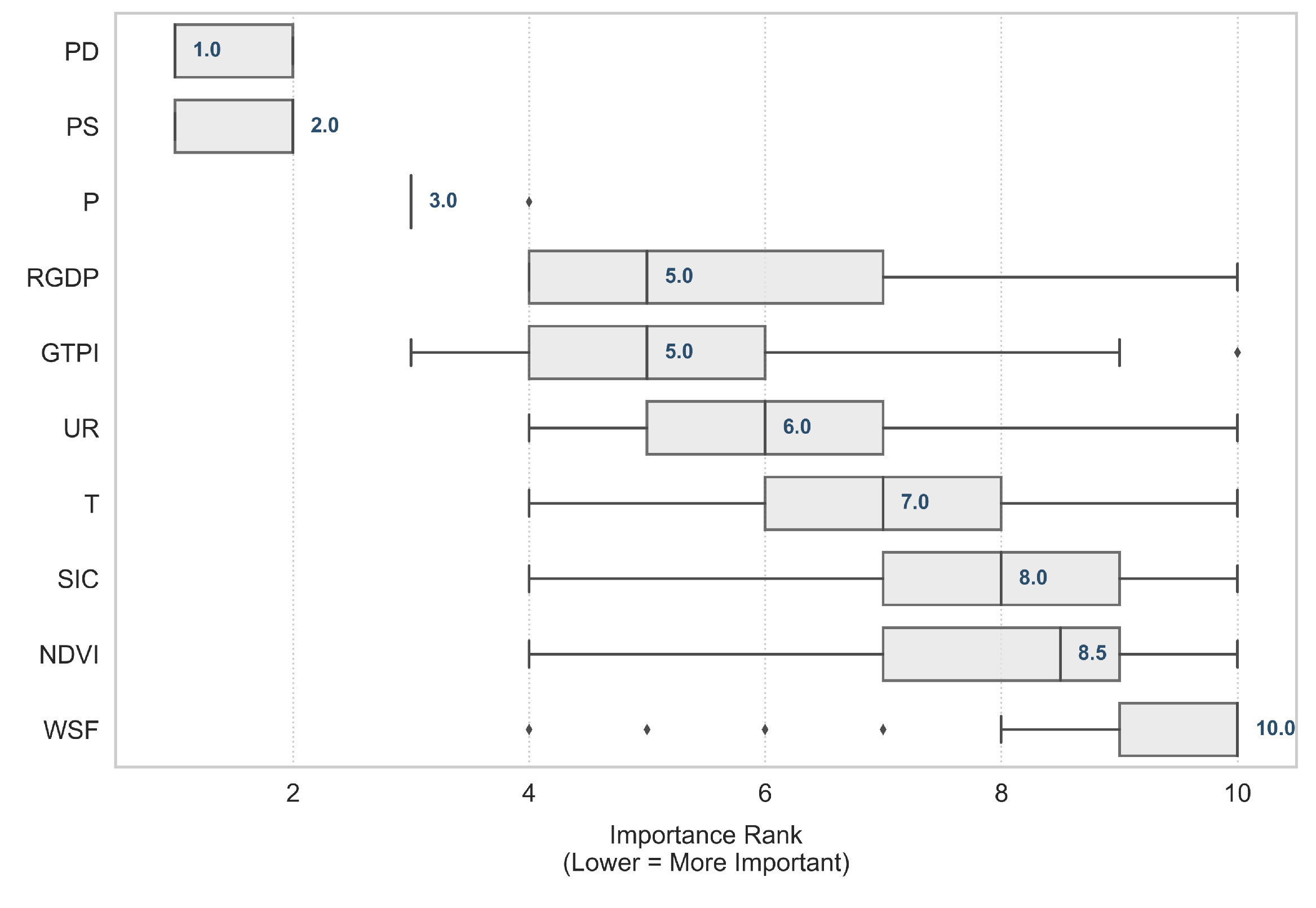
    Second, a bootstrap resampling procedure (B = 500) evaluated the stability of driver importance rankings. The median rank ( R j ˜ ) and interquartile range (IQR) across iterations identified consistent global drivers:
    R j ˜ = median r j ( b ) b = 1 B
    IQR j = Q 3 ( r j ) Q 1 ( r j )
  • Spatial heterogeneity analysis
    Regions exhibiting high prediction errors (e.g., Region 2 in Fold 3, R 2 = 0.055 ) were analyzed to uncover localized mechanisms. Welch’s t-tests and Cohen’s d effect sizes quantified feature differences between anomalous and typical regions:
    d = X ¯ 1 X ¯ 2 s pooled , s pooled = ( n 1 1 ) s 1 2 + ( n 2 1 ) s 2 2 n 1 + n 2 2
    where X ¯ 1 and X ¯ 2 denoting group means, and s 1 and s 2 denoting their standard deviations. This analysis characterized the unique socio-ecological profiles leading to spatial heterogeneity in emissions.
A suite of specialized software tools was employed to ensure robust and state-of-the-art analysis. A comprehensive overview of these tools, justifying their selection and outlining their specific contributions, is available in Appendix C.

3. Results

3.1. Land Use Changes in Shanxi Province

3.1.1. Rates of Land Use Change

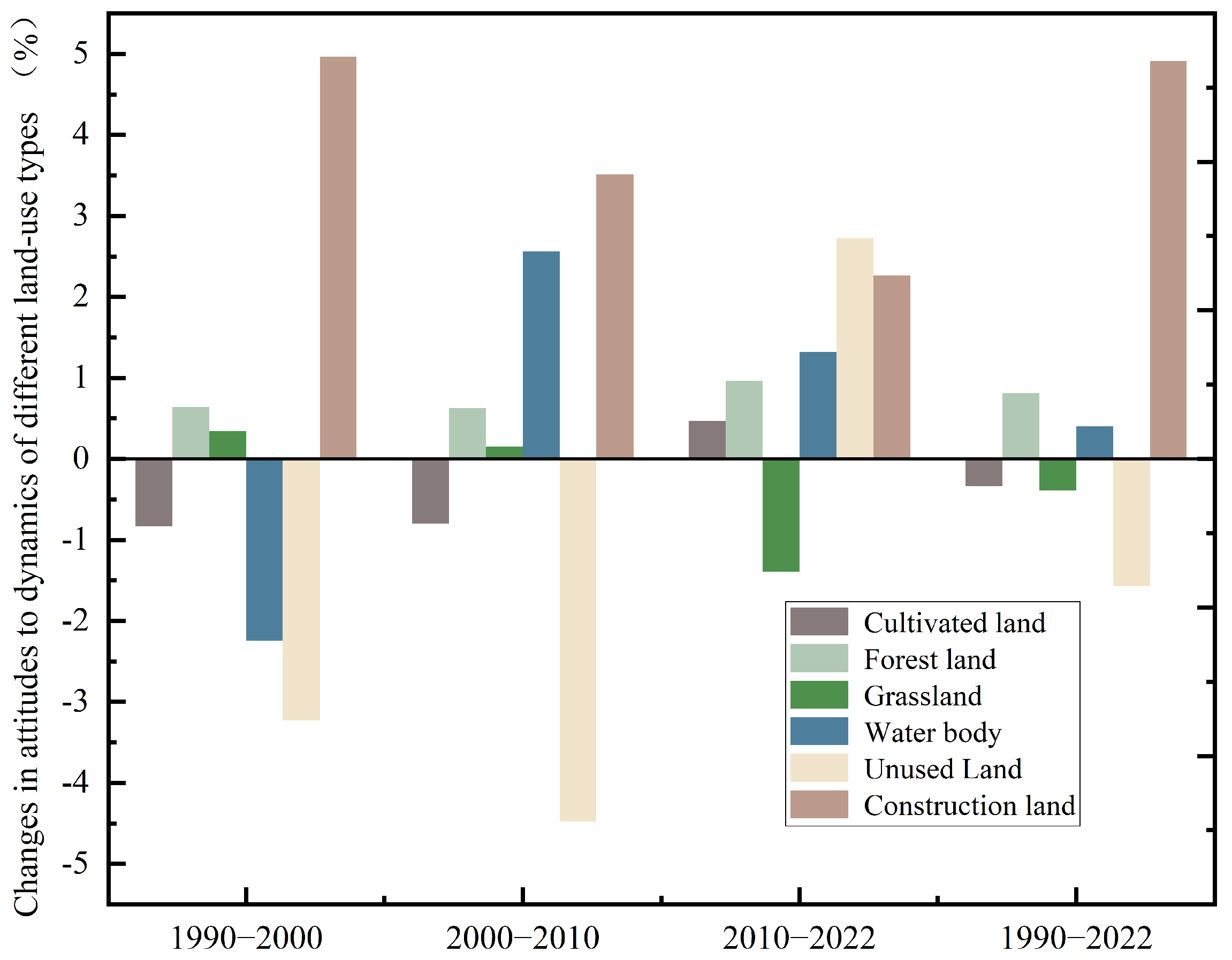
Land use dynamics from 1990 to 2022 were quantified through individual and composite dynamic degree using ArcGIS for spatial analysis and calculation (Figure 3). Construction land showed the highest dynamic degree (4.96%) during 1990–2000, declining to 2.26% in 2010–2022, yet remaining the most dynamic type overall. This slowdown reflects stricter land supply controls, anti-speculation measures, and a strategic shift from expansion to stock optimization under policies like the Linking Increase with Decrease” mechanism [47] and idle land crackdowns [48,49,50].
Unused land decreased notably ( 0.80 % ) during 2000–2010 but rebounded slightly ( + 0.47 % ) afterward. This shift resulted from the “Linking Increase with Decrease” policy, creating incentives for quota reserves [51], the growing prioritization of stock revitalization [52], and enhanced ecological protection that restricted development on fragile terrains.
Grassland dynamism turned negative ( 1.39 % ) after 2010, indicating sustained shrinkage under grazing bans and ecological restoration policies [53,54]. Forest land increased from 0.64% to 0.96%, reflecting gains from large-scale afforestation and the “Grain-for-Green” program [55,56]. Cultivated land remained relatively stable ( 0.34 % ) due to the strict farmland protection system and enforcement of the basic farmland red line [57,58].
These distinct trajectories—expansion of construction and forest land, alongside shrinkage of grassland, unused, and cultivated land—illustrate Shanxi’s evolving balance between ecological recovery and development.

3.1.2. Structural Changes in Land Use

Land use transition patterns and net changes in land use types in Shanxi Province from 1990 to 2022 were analyzed based on a land use transfer matrix derived from ArcGIS, with the results visualized using a Sankey diagram and a bubble chart in Figure 4. The Sankey diagram illustrates land use conversions among six categories during 1990–2000, 2000–2010, and 2010–2022. Cultivated land exhibited the largest reduction, mainly converted to grassland and construction land. Grassland showed bidirectional shifts with cultivated and forest land, reflecting the combined influences of agricultural development and ecological restoration programs. Forest land expanded steadily, largely replacing grassland and cultivated land. Construction land increased continuously, encroaching on cultivated and forest areas. Water bodies and unused land remained relatively stable.
The Sankey bubble chart illustrates the net changes in land use types from 1990 to 2022. The size of each bubble reflects the absolute magnitude of land use change, while color indicates whether the change is positive or negative. Over this period, the areas of cultivated land and grassland experienced notable declines of 7.199   ×   10 5   h a and 6.696   ×   10 5   h a , respectively. In contrast, forest land and construction land expanded significantly by 8.782   ×   10 5   h a and 5.064   ×   10 5   h a . The most pronounced reduction in grassland occurred between 2010 and 2022, with a net loss of 9.347   ×   10 5   h a , while forest land saw its largest increase of 4.392   ×   10 5   h a during the same period—highlighting a substantial conversion from grassland to forest. Changes in water bodies and unused land remained relatively minor throughout the study timeframe. Overall, these patterns reflect the combined impacts of ecological restoration and urban expansion on regional land systems, emphasizing the importance of coordinated and sustainable land use planning.

3.2. Temporal Characteristics of Land Use Carbon Emission

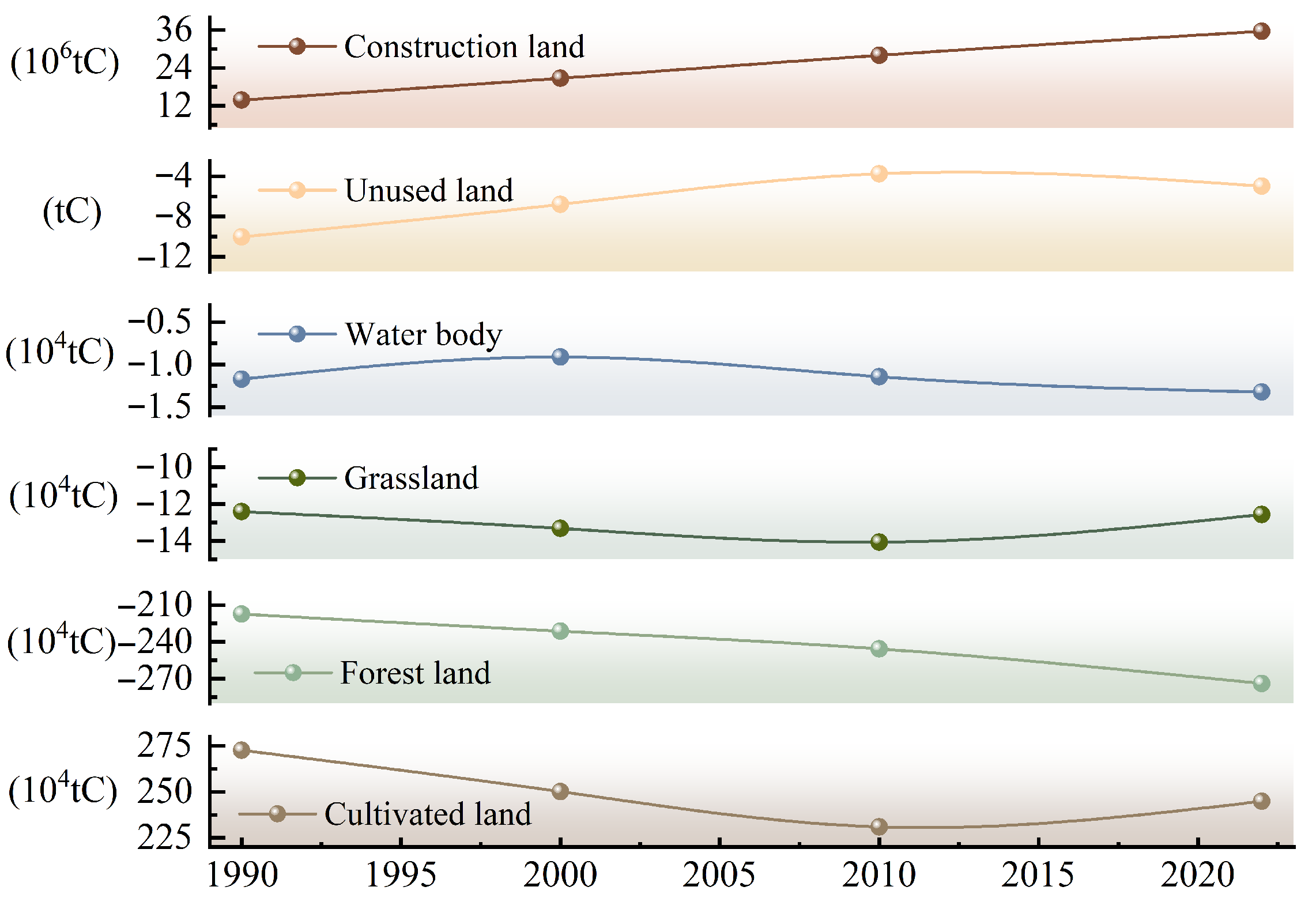
Carbon emissions and sinks showed distinct trajectories across land types in Figure 5, as calculated using a carbon emission model. Emissions from cultivated land decreased from 272.61 × 10⁴ tC in 1990 to 231.02 × 10⁴ tC in 2010, before rebounding slightly to 244.90 × 104 tC by 2022. Emissions from construction land increased steadily throughout the period, rising from 13.85 × 10⁶ tC in 1990 to 35.61 × 10⁶ tC in 2022, becoming the dominant contributor to total emissions, driven by continued urbanization and industrial growth.
Forest land saw a steady increase in sequestration capacity, from 217.42 × 10 4 tc in 1990 to 273.98 × 10 4 tc in 2022, reflecting enhanced forest carbon sinks driven by ecological policies and vegetation recovery. Grassland emissions remained relatively stable, decreasing slightly from −12.40 × 10⁴ tc to −12.56 × 10⁴ tc over the same period. Water bodies and unused land showed only minor changes in their carbon sink capacities, with unused land changing from −10.04 tc in 1990 to −4.98 tc in 2022.
Despite some mitigation progress, the sharp increase in emissions from construction land continued to drive provincial carbon growth, underlining the challenges of reconciling rapid development with low-carbon objectives. The structure of emissions shifted markedly toward construction land, while the weakening of forest carbon sinks further undermined the regional carbon balance, and Shanxi province’s low-carbon transition remains under significant pressure.

3.3. Spatial Distribution Characteristics of Land Use Carbon Emission

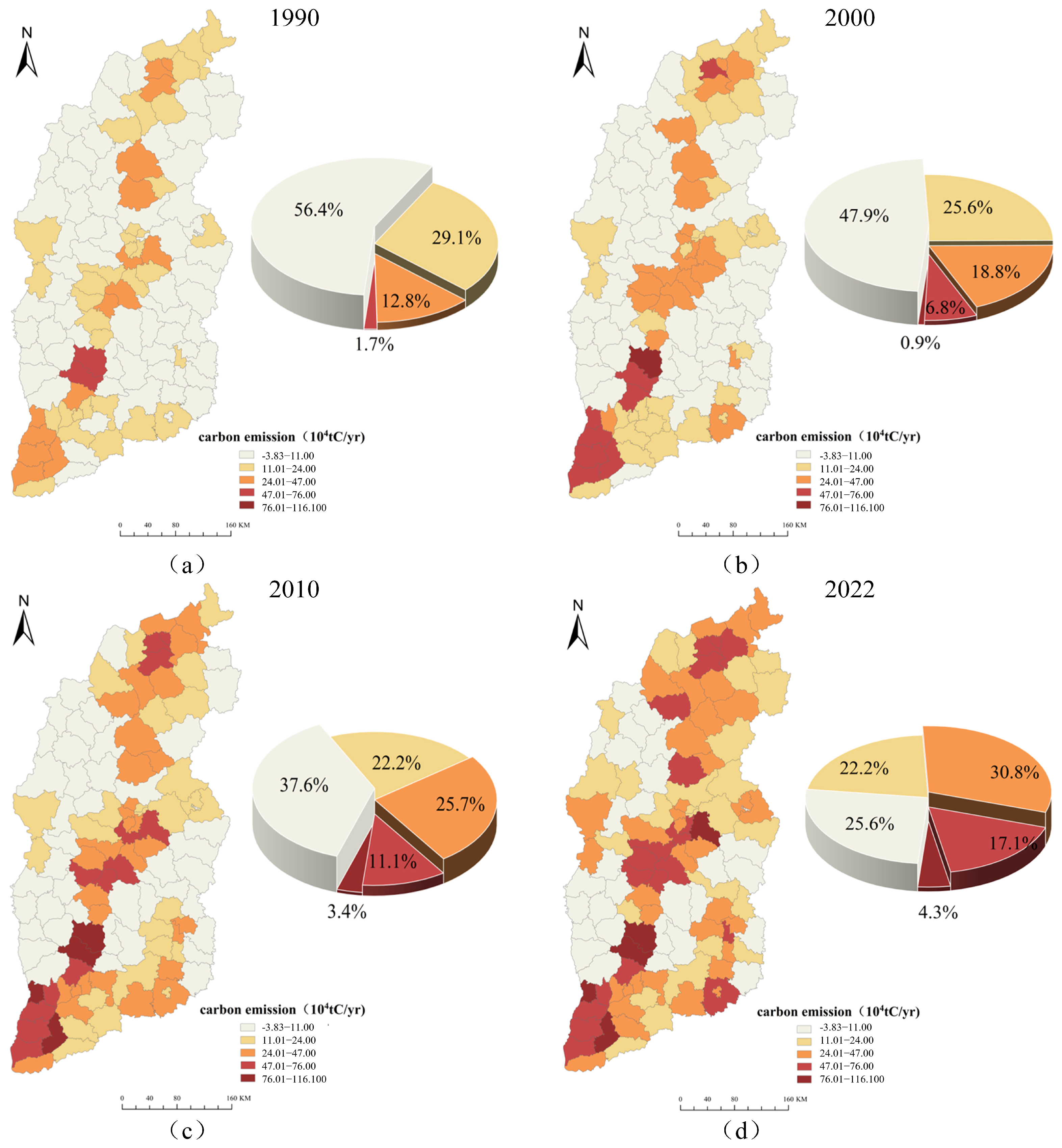
The spatial distribution of county-level carbon emissions in Figure 6 exhibits pronounced spatiotemporal heterogeneity and a progressively intensifying trend across Shanxi Province. Overall, county emissions follow a “high in the northeast and low in the southwest” pattern, evolving from scattered distributions to clustered regional hotspots. Low-emission counties are predominantly located near the Taihang and Lvliang Mountain ranges, contrasting with elevated emissions concentrated in five major basins: Yuncheng, Linfen, Taiyuan, Xinding, and Datong. Over time, emission cores at the county scale gradually merged into larger contiguous clusters.
In 1990, county-level emissions were generally low and spatially dispersed. By 2000, emission intensity increased significantly in central and southern counties, transitioning from isolated point sources to multi-county clusters driven by economic expansion. By 2010, high-emission counties coalesced into continuous zones across central-southern Shanxi. By 2022, emission hotspots expanded both northward and southward at the county scale, peaking in central-southern basins and northern regions. The maximum spatial extent and intensity of county emissions occurred in 2022, underscoring persistent challenges linked to county-level land use patterns.
From 1990 to 2022, the proportion of counties classified as low emission decreased significantly from 56.4% to 25.6%, while the relatively low emission category declined slightly from 29.1% to 22.2%. In contrast, medium emission counties increased notably from 12.8% to 30.8%. More importantly, counties categorized as relatively high emission rose sharply from 1.7% to 17.1%, and high emission counties emerged from 0.0% to 4.3% over the same period. These trends demonstrate a clear spatial shift of county-level carbon emissions toward higher intensity categories, indicating growing emission hotspots and heightened challenges for differentiated carbon management and regional climate mitigation policies.
The spatiotemporal evolution of LISA clusters from 1990 to 2022 reveals profound shifts in the spatial structure of [insert variable, e.g., carbon emissions/carbon efficiency] across Shanxi Province, signaling a significant regional transition (Figure 7).
The most pronounced trend is a definitive north-south reversal in spatial dominance. During the 1990s, High-High clusters were present in both northern and southern regions, indicating intensified core activity. By 2022, however, northern High-High clusters had diminished, while southern Low-Low clusters became more persistent, marking the formation of a stable low-value zone and reflecting substantial spatial reorganization.
Spatial outliers also show transformative dynamics: non-significant areas dominated throughout, indicating basic stability. Low-Low outliers consistently clustered in central Jinzhong, suggesting structural constraints. After 2000, High-Low outliers disappeared entirely, signaling spatial convergence. Low-High outliers shifted from southwestern to southern Shanxi, and by 2022, new High-Low outliers emerged in the north—indicative of weakening regional dominance.
Persistent southern High-High clusters, central Low-Low zones, and emerging northern outliers together highlight intensified spatial differentiation, forming a core-periphery structure. Key drivers include regional policy bias, natural resource trends, uneven infrastructure, environmental constraints, and labor reorganization. This pattern reveals not just north-south divergence, but a profound provincial restructuring, offering critical insights for addressing regional inequality. The formation of these stable spatial clusters, driven by regional policy bias and natural resource trends, underscores the necessity for differentiated carbon governance strategies tailored to the specific socio-ecological profile of each region.

3.4. Comprehensive Evaluation of Carbon Emission Efficiency Considering Environmental Factors

3.4.1. Empirical Results of the Stage 1 SBM Analysis

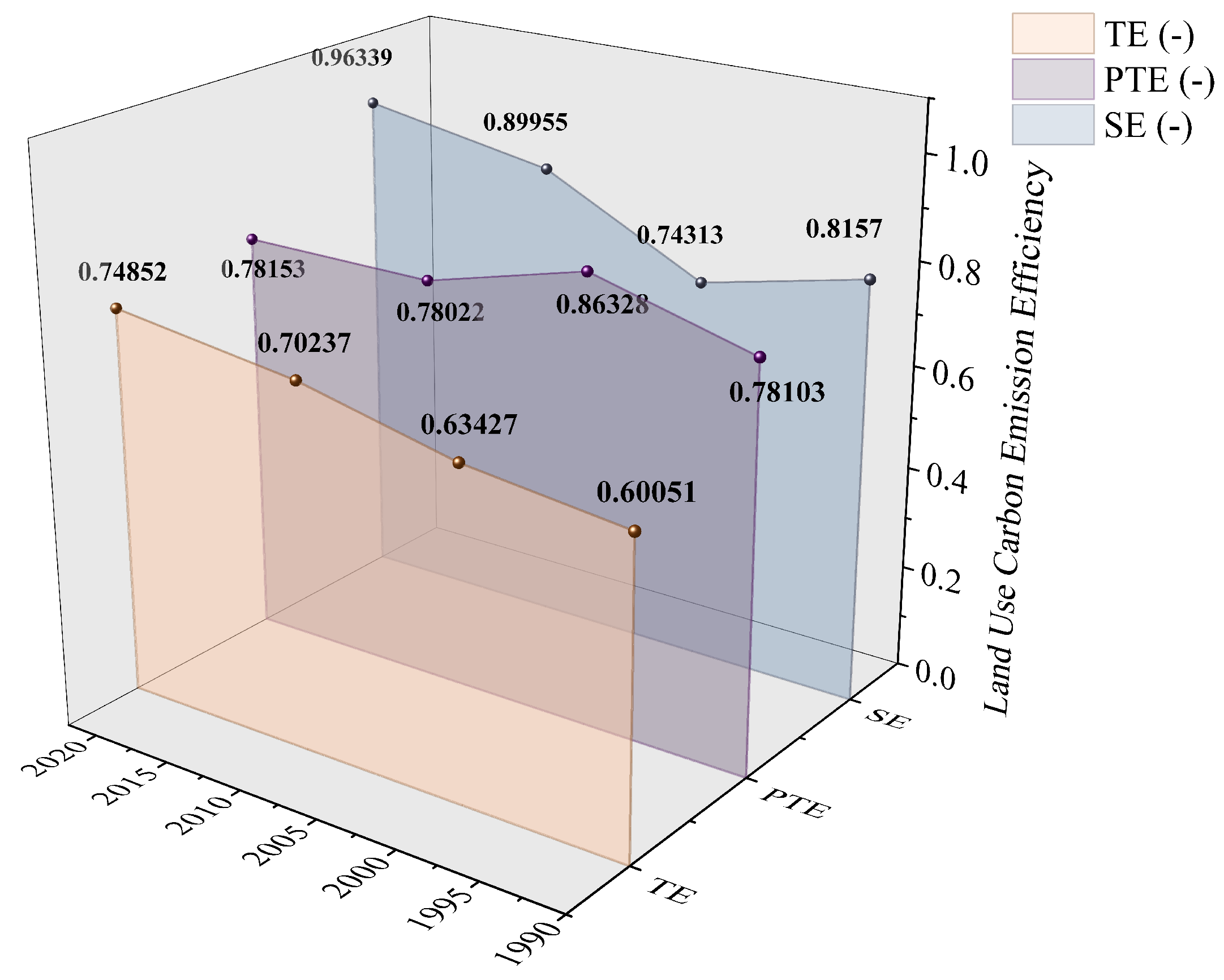
An analysis of LUCE efficiency in Shanxi Province from 1990 to 2022 was conducted using an SBM-DEA model with multi-input and undesirable output parameters (Figure 8). Technical Efficiency (TE) increased from 0.6005 to 0.7485, indicating improved carbon emissions management. Pure Technical Efficiency (PTE) remained largely unchanged, reflecting limited technological progress. In contrast, Scale Efficiency (SE) rose markedly from 0.8157 to 0.9634, accounting for 89.3% of the total efficiency gains. These results suggest that improvements were primarily driven by scale expansion rather than technological innovation. To improve accuracy, the initial SBM-DEA results were further analyzed using an SFA to control for the influence of external environmental factors and stochastic noise, following standard efficiency measurement procedures to enhance reliability.

3.4.2. Results and Analysis of Stage 2 SFA Regression

This study used SFA with Frontier 4.1 to regress Stage 1 input slack variables against six environmental covariates (Table 5). All γ values above zero confirm the validity of the frontier function specifications. The likelihood ratio test for one-sided errors was significant at the 10 % level, supporting the effectiveness of the SBM-DEA framework in isolating environmental influences.
Urbanization exerts divergence across productive dimensions. Urbanization significantly enhances capital stock efficiency and labor productivity, consistent with agglomeration economies optimizing resource allocation [59]. In contrast, its impact on land use demonstrates weaker alignment with carbon efficiency goals. The positive but statistically insignificant coefficient for land input suggests urban spatial expansion correlates with elevated carbon intensity per land unit. This pattern likely stems from two systemic constraints: excessive conversion of non-construction land and suboptimal spatial configurations that increase energy demands. These findings necessitate differentiated policy interventions that preserve the advantages of urban growth in capital and labor while enforcing land use controls to encourage compact development and low-carbon infrastructure.
The analysis revealed distinct patterns in how government intervention affects different input dimensions. A significant negative coefficient for land input slack (−0.6164, significant at the 1% level) indicates that government intervention plays a key role in improving land resource efficiency, likely through policies promoting land remediation, environmental regulation, and infrastructure investment [60]. Although its effects on capital and labor input slack were statistically insignificant, government-led resource coordination may still indirectly support factor efficiency. Moreover, enhanced land governance contributes to lower carbon emissions per unit land use, thereby fostering improvements in LUCE. These findings suggest that although government intervention primarily exerts a direct influence on land use efficiency, it also functions as a critical lever in achieving broader low-carbon development goals [61].
Economic development level exhibited contrasting effects across input dimensions. Significant negative coefficients of −0.1639 (1% level) and −0.1283 (5% level) were found in capital stock and labor input slack, indicating that current economic growth is associated with excessive input and inefficiency. This aligns with the trade-offs observed by Wang and Wang (2019), who noted that heightened economic growth constrained carbon emission efficiency improvements [62]. In the land use dimension, the coefficient was statistically insignificant, reflecting a mismatch between economic expansion and effective land use under existing planning frameworks. These results suggest LUCE remains sensitive to growth modes: while development could enhance efficiency via green technology and industrial upgrading, the region may still lie on the ascending side of the environmental Kuznets curve, where rising activity lowers LUCE.
The analysis showed varying impacts of GTPI across production dimensions. In the labor input dimension, GTPI had a significant positive effect (0.0880, p < 0.05 ), suggesting that green innovation enhances labor efficiency through skill-based technological change, human-capital upgrading, improved workforce allocation, enhanced operational practices, better integration of green skills into employment structures, and increased adaptability to technological shifts. However, its impact on capital stock and land use slack was statistically insignificant, indicating that decarbonization in these areas still relies on broader institutional innovations, stronger policy coordination, improved regulatory frameworks, consistent technology diffusion, and supportive financial mechanisms. The lack of effect on land use suggests green innovation has yet to drive notable LUCE improvement.
Population density exhibited distinct effects, showing a significant negative coefficient (−0.2221, p < 0.05 ) in labor allocation. This negative correlation suggests that agglomeration may intensify labor market pressure, leading to reduced LUCE. No significant associations were identified in the capital and land dimensions. This indicates that population concentration does not currently translate into measurable changes in capital use or land resource allocation. The results highlight the importance of targeted spatial governance. Reducing labor market saturation in densely populated areas and improving capital circulation and land use planning may help mitigate efficiency losses and support LUCE improvement.
Industrial restructuring showed no statistically significant effects on capital, labor, or land use efficiency ( p > 0.1 ). Although the coefficient for land use in the secondary industry was 0.177, the lack of significance suggests that current restructuring efforts have not addressed rigidities in factor markets or existing technological paths. The absence of significant effects across all inputs indicates that fragmented industrial policies may not effectively remove the structural barriers limiting low-carbon transformation. Achieving substantial emission reductions may require coordinated measures that target technological inertia, labor market mismatches, and inefficiencies in land management. Moreover, without integrated planning, sectoral shifts risk creating new inefficiencies. Stronger alignment between economic restructuring and spatial governance is essential to unlock synergistic decarbonization potential.
Overall, UR and GOV drive LUCE improvements by optimizing capital and labor use and reducing land slack. Resource-intensive economic growth currently hinders LUCE in both capital and labor dimensions. Green technology progress boosts labor efficiency but not capital or land use, while population density reduces LUCE via labor market congestion, and industrial restructuring shows no significant effect. Integrated policies aligning economic growth, spatial planning, and innovation are needed to advance low-carbon land use.

3.4.3. Analysis of Adjusted SBM Results

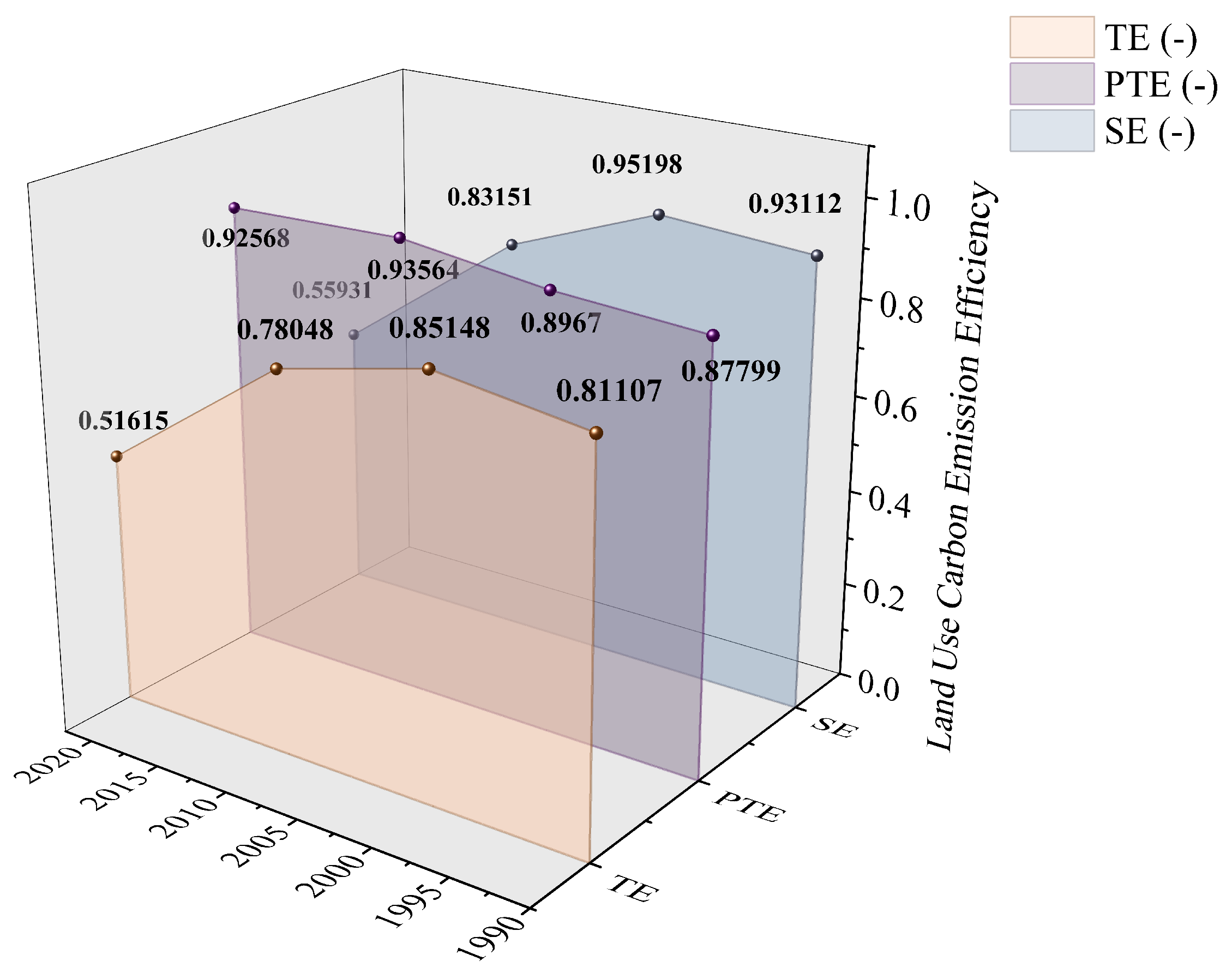
The SBM model was reimplemented using SFA-adjusted inputs and the original outputs to assess LUCE, as shown in Figure 9. LUCE demonstrated substantial volatility. Initial measurements in 1990 showed TE, PTE, and SE at 0.8111, 0.8780, and 0.9311, respectively, indicating comparatively optimal LUCE. By 2000, TE and SE rose to 0.8515 and 0.9520, suggesting continued efficiency gains. A marked decline occurred by 2010, with TE and SE falling to 0.7805 and 0.8315, potentially associated with economic restructuring impacts on resource allocation. The most recent 2022 data revealed TE and SE at 0.5161 and 0.5593, signaling persistent efficiency challenges. In contrast, PTE maintained stable growth throughout the study period, advancing from 0.8780 to 0.9257, demonstrating sustained technological contributions to carbon efficiency enhancement.

3.4.4. Comparison of Stage 1 and Stage 3 Efficiency Scores Across Cities

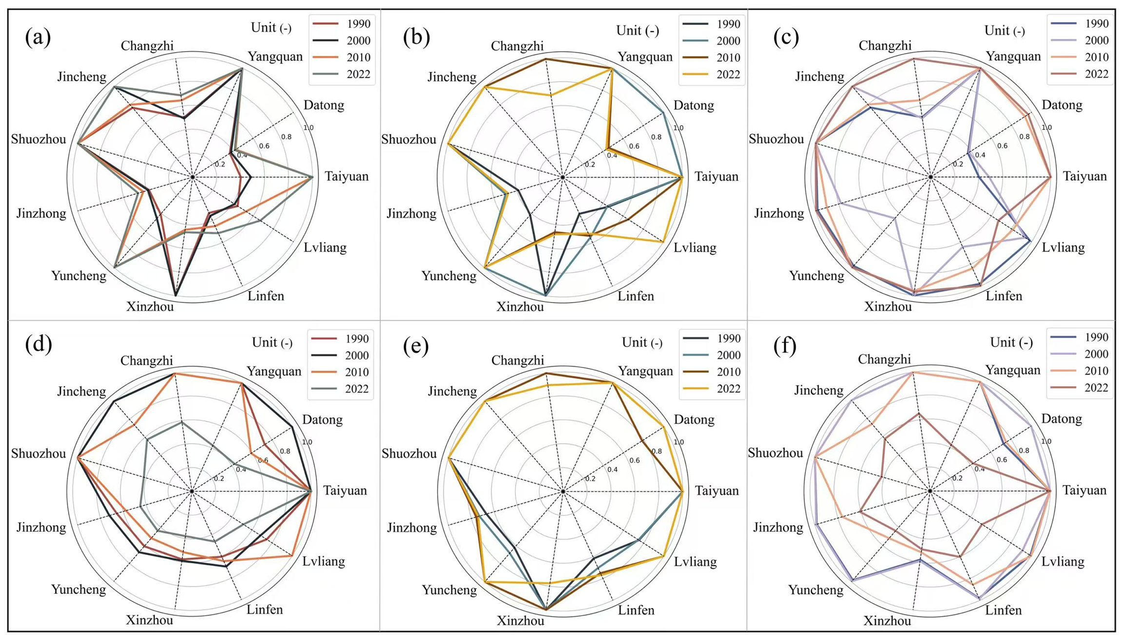
Figure 10a–f present the temporal evolution of TE, PTE, and SE across 11 cities in Shanxi Province from 1990 to 2022. The divergence between Stage 1 and Stage 3 results after 2010 reveals important insights into China’s macroeconomic policies. While Stage 1 results show apparent stability, with five fully efficient cities (TE = 1) in both 2000 and 2022, Stage 3 results uncover a sharp decline from seven efficient cities in 2000 to just Taiyuan by 2022.
This pattern represents an investment-driven growth paradox. The post-2008 stimulus package, reliant on massive credit expansion, initially boosted output in resource-rich provinces like Shanxi, inflating the raw Stage 1 efficiency metrics. The Stage 3 analysis reveals that this growth model subsequently induced severe structural imbalances. The adjustment process unmasked an important reality: early unfavorable conditions had hidden true managerial efficiency (evidenced by high initial Stage 3 PTE), whereas, by 2022, the apparent efficiency of cities like Yangquan and Shuozhou was revealed to be dependent on external favors rather than excellent management.
Period decomposition (Table 6) shows how efficiency drivers have shifted over time. TE improvements around 2000 were primarily driven by scale efficiency gains, as seen in rising SE values in both stages, indicating that external factors initially helped achieve scale economies. Post-2010, Stage 3 results reveal a scale efficiency crisis, with SE values plummeting to 0.42–0.65 by 2022, quantifying the severe overcapacity in traditional industries and inefficient urban expansion fueled by investment-led growth.
Notably, PTE remained high and stable across stages and models ( ρ = 0.85 ), confirming that core managerial practices and technological application were robust. This stability indicates a predictable response to policy instruments. However, these improvements in pure technical efficiency were overwhelmed by massive losses from structural misallocation, as captured by the plunging Stage 3 SE.

3.4.5. Robustness Checks

Multiple robustness checks were implemented to enhance the credibility of the findings and to address key methodological concerns and parameter uncertainties.
Water-body-neutral scenario: Given that the treatment of water bodies as a carbon sink constitutes a major assumption and potential source of uncertainty, a conservative scenario was constructed by setting their net carbon flux to zero. The resulting city efficiency rankings were highly consistent with those from the baseline scenario, thereby confirming the stability of the comparative findings. Spearman’s rank correlation analysis further demonstrated strong and statistically significant associations for TE, PTE, and SE across all study years (average ρ > 0.80 , p < 0.01 ). Detailed efficiency scores and the complete correlation analysis are reported in Appendix A.
Reclassifying land variables: To address the potential for mechanical linkage between land inputs and emission outputs, a key robustness check was performed by reclassifying land composition variables as environmental variables in the second-stage SFA. While this specification change significantly affected the absolute values of the efficiency scores—as theoretically expected when altering the production frontier—the relative performance rankings of cities remained highly stable. Table 7 summarizes the changes in descriptive statistics and the high rank correlations. Spearman’s rank correlation coefficients between the original and alternative rankings were strong and significant for TE, PTE, and SE across all study years (average ρ > 0.91 , p < 0.001 ). This confirms that our core findings regarding inter-city performance disparities are robust to this fundamental model respecification.
Spatial dependence analysis: The estimation of the Spatial Error Model (SEM) yielded a statistically significant spatial error coefficient ( λ = 0.27 , p = 0.012 ). This result confirms the presence of substantive residual spatial autocorrelation, implying that unobserved shocks or factors influencing input slacks spill over across city boundaries, as defined by our first-order Queen contiguity weights matrix.
However, despite this statistical evidence of spatial dependence, adjusting for it through the SEM led to only negligible changes in the computed efficiency scores and their ordinal rankings. The robustness of the initial estimates is underscored by the near-perfect correlation between the original and spatially adjusted scores for TE (TE, ρ = 0.973 ), PTE (PTE, ρ = 0.847 ), and SE (SE, ρ = 0.900 ) (all correlations significant at p < 0.001 ).
Monte Carlo uncertainty analysis: To provide a compact overview of the uncertainty in our core efficiency measures, we employed a Monte Carlo simulation with 1000 iterations to perturb land use carbon emission coefficients within their plausible ranges. Table 8 reports the 5th (p5), 50th (median, p50), and 95th (p95) percentiles for TE and SE across all cities in Shanxi Province for 2022.
As shown in Table 8, two key patterns emerge: (1) the median (p50) efficiency values provide robust central estimates for cross-city comparisons, and (2) SE exhibits substantially wider uncertainty bands than TE, as indicated by the median Inter-Percentile Range (IPR). This differential sensitivity, revealed by the Monte Carlo simulation, aligns with our interpretation that scale-related inefficiencies are both a major driver of performance decline and inherently more sensitive to parameter uncertainty. Full uncertainty results for all benchmark years and efficiency measures are reported in Appendix B.

3.5. Drivers of Land Use Carbon Emissions

3.5.1. Global Model Performance and Robust Driver Identification

The globally calibrated XGBoost model demonstrated a satisfactory capability to explain land use carbon emissions, providing a baseline understanding of the dominant drivers. The bootstrap resampling analysis ( n = 500 iterations) was then employed to evaluate the statistical stability of the feature importance rankings derived from this global model.
As depicted in Figure 11, population-related indicators (POPD and POPS) consistently emerged as the two most important and robust drivers across all bootstrap samples, exhibiting the lowest median ranks (1.5 and 2.1, respectively) and the narrowest distributions (IQR < 1.0). This confirms that their dominant influence is a statistically sound finding. RGDP also demonstrated stable high importance (median rank = 3.2, IQR = 1.5). In contrast, the importance of natural endowment variables (e.g., NDVI, P) exhibited greater variability, underscoring their secondary and context-dependent role.

3.5.2. Interaction Effects Among Robust Drivers

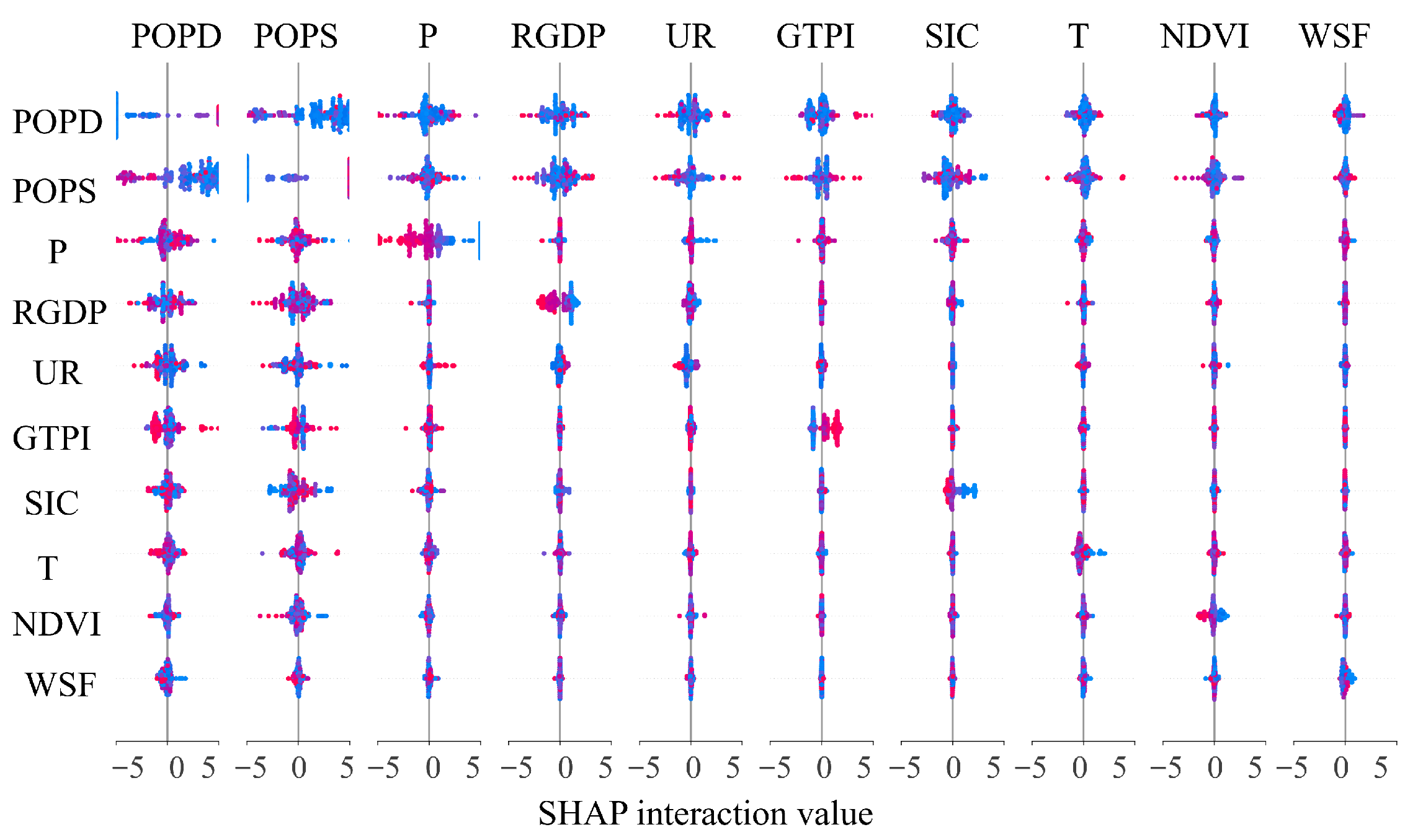
To systematically assess the associations between different factors and land use carbon emissions, this study applied XGBoost modeling in combination with SHAP analysis. SHAP interaction values were calculated to decompose the total marginal contribution of features into main and interaction effects within the model, quantifying how the presence of one feature modifies the predictive effect of another.
As shown in Figure 11, population-related indicators (POPD and POPS) were identified as the strongest predictive features. Figure 12 further reveals that the interaction between POPD and POPS was the most prominent, exhibiting strongly positive joint effects within the model. When both variables were high, interaction values rose sharply, suggesting that densely populated and highly concentrated areas are associated with disproportionately higher carbon emissions in the model output. This pattern may be linked to increased residential energy demand, transportation intensity, and land development. RGDP also showed a clear upward trend in marginal contribution. Notably, its strong positive interaction with POPD indicates an economic agglomeration pattern within the model: high population density is associated with amplified emission predictions concurrent with economic production intensity, while economic indicators correlate with infrastructure-related emissions.
In contrast, NDVI had minimal interaction effects in the model, as regional vegetation coverage shows limited predictive interplay with other features in offsetting emission patterns concentrated in urban centers. Certain other feature combinations revealed discernible joint effects. For instance, high values of both RGDP and P were associated with stronger predicted emissions, possibly reflecting correlated land use intensification under favorable conditions. Interactions between GTPI and SIC appeared to moderate predicted emissions, suggesting a potential mitigating role of technological factors in the modeled relationships.

3.5.3. Spatial Heterogeneity and Model Transferability Assessment

To assess the spatial transferability of the global model and the universal applicability of the identified drivers and their interactions, spatial k-fold cross-validation was implemented.
The results revealed pronounced spatial heterogeneity. As summarized in Table 9, the average out-of-sample performance across all folds was R 2 = 0.550 and RMSE = 12.783. Crucially, Fold 3 (Region 2) exhibited a severe decline in predictive performance ( R 2 = 0.055 ) with the highest RMSE (16.602), indicating a fundamental breakdown of the global model’s learned mechanisms in this region.
To diagnose the anomaly in Region 2, a comparative analysis of its socio-ecological profile was conducted. As summarized in Table 10, Region 2 exhibits significantly elevated anthropogenic pressures (WSF: +15.0%; UR: +11.2%) coupled with severely depleted natural endowment (NDVI: −35.7%; P: −25.7%; T: −26.2%). Welch’s t-tests confirmed these differences were highly significant ( p < 0.001 ) with large effect sizes (Cohen’s d > 0.8 ).

3.5.4. Synthesis: Global Patterns and Local Exceptions

This spatial heterogeneity presents a critical nuance: while POPD, POPS, and RGDP were identified as the most globally robust drivers, with their interactions defining the dominant global emission patterns, their influence fails locally in specific regions like Region 2. This does not invalidate the global findings but precisely defines the boundaries of their applicability. Consequently, while the global model informs broad-scale policy, region-specific mitigation strategies are essential, particularly for anomalous regions requiring tailored approaches beyond the global narrative.

4. Discussion

4.1. Spatiotemporal Changes in Land Use Carbon Emission

This study analyzed spatiotemporal patterns of land use change and carbon emissions in Shanxi Province using the China Land Cover Dataset (CLCD) from the Wuhan University Huang Xin team. Derived from Landsat imagery, the CLCD provides a 30 m spatial resolution, annual temporal continuity, and open access with high spatiotemporal consistency. The results indicate increased forest land, water bodies, and construction land, alongside decreased cultivated land, grassland, and unused land. These findings differ partly from earlier studies, especially in relation to the expansion of water bodies. Discrepancies may stem from differing study periods, data sources, or methodologies. The increase in water bodies is likely associated with improvements in water conservancy infrastructure, the implementation of ecological restoration policies, and regional climate shifts. These factors collectively reflect enhanced water management efforts.
For carbon emission accounting, this study adopted the emission coefficient method to estimate both direct and indirect emissions from land use change due to the absence of long-term, detailed data on energy consumption and agricultural activities. The results showed a steady annual increase in land use carbon emissions, consistent with previous research. This approach effectively captured historical spatiotemporal trends in emissions associated with land use and cover change, offering a solid basis for refining land use strategies and promoting low-carbon development. Furthermore, the spatial emission patterns identified here, especially the clustering of high emissions in industrial counties, establish a critical baseline for prioritizing targeted mitigation strategies. These results provide an essential spatial framework for future work on energy structure optimization and the strategic deployment of carbon capture, utilization, and storage (CCUS) infrastructure in Shanxi’s key industrial regions.

4.2. Three-Stage SBM-DEA Methodology

The Stage 3 efficiency results in Shanxi Province remain robust, confirming that city rankings are largely unaffected by residual spatial dependence or mechanical linkage. The divergence between Stage 1 and Stage 3 highlights an investment-driven growth paradox: while raw efficiency metrics appeared stable, controlling for environmental factors reveals a sharp decline after 2010, reflecting overcapacity and structural imbalances induced by post-2008 stimulus policies.
Driver analysis indicates differentiated effects of socio-economic and technological factors. Government intervention and urbanization enhanced land use efficiency via improved resource allocation and regulatory enforcement, whereas high GDP growth in energy-intensive regions exerted negative pressure on efficiency. Green technology progress has improved labor efficiency but has yet to produce broad impacts across industrial processes.
These findings demonstrate the necessity of a three-stage framework to disentangle managerial inefficiency, environmental heterogeneity, and statistical noise. The resulting city rankings, derived from the primary SFA-adjusted Stage 3 analysis, prove robust to residual spatial dependence—a finding confirmed by SEM adjustments that, despite significant spatial error, yield materially unchanged ranking orders. This consistency provides a solid foundation for targeted policy interventions and highlights key levers for promoting low-carbon development in resource-dependent provinces.
Furthermore, the robustness of these findings is substantiated by a comprehensive Monte Carlo uncertainty analysis (Table 8). Despite introducing substantial perturbations (±30%) to the underlying land use emission coefficients, the relative performance rankings of cities remained highly stable (average Spearman’s ρ > 0.91). Crucially, this exercise confirmed that SE—the primary driver of the post-2010 efficiency decline—is inherently more sensitive to parameter uncertainty than TE, yet its median estimates robustly uphold the conclusion of significant scale misallocation. This demonstrates that the core policy implications regarding investment-driven overcapacity are not an artifact of statistical uncertainty but reflect a persistent structural issue.

4.3. Drivers of Land Use Carbon Emissions

This study identifies multiple prominent predictive features associated with land use carbon emissions in Shanxi Province and rigorously assesses their robustness and spatial stability. The bootstrap resampling analysis ( n = 500 ) first established that POPS and POPD are the most stable and dominant predictors, exhibiting the lowest median importance ranks and smallest variance across iterations. This finding confirms the statistical robustness of their predictive power and is consistent with findings by Guo et al. (2024) [63]. Similarly, RGDP was consistently identified as a robust high-impact predictor, aligning with the strong associative influence reported by Udemba et al. (2022) [64], particularly in high-income regions. It is important to note that in the context of Shanxi Province, the industrial structure variable serves as a robust proxy for its coal-dependent energy pattern, as secondary industry expansion is intrinsically linked to increased coal consumption. This conceptual linkage helps capture the core influence of energy structure on carbon emissions, despite the lack of direct energy data at the prefecture level. The interaction between economic development and natural conditions, such as precipitation, further intensified emissions in high-value areas, reflecting the compounded influence of economic and environmental factors, as also observed by Qu et al. (2023) [65].
A crucial finding of this study is the pronounced spatial heterogeneity in these predictive relationships, which was uncovered through spatial cross-validation and subsequent statistical interrogation. The case of Region 2 exemplifies a specific archetype—“High Anthropogenic Intensity—Low Natural Endowment”—where Welch’s t-tests and Cohen’s d effect sizes confirmed statistical significance ( p < 0.001 ) and substantial deviations in multiple features (e.g., WSF: +15.0%, NDVI: −35.7%) from the regional mean. This extreme socio-ecological profile explains why the conventional global model fails here due to fundamentally distinct local predictive mechanisms, a conclusion strengthened by the combination of spatial validation and statistical testing.
Theoretically, this underscores the critical perils of spatial non-stationarity. The demonstration that globally robust predictors (via Bootstrap) can fail locally (via Spatial CV) provides a compelling case that ignoring geographical heterogeneity can lead to model misspecification and severely biased inferences. Practically, it argues compellingly against the sufficiency of uniform, province-wide policy approaches. Mitigation strategies in anomalous regions like Region 2 must be highly targeted, de-emphasizing reliance on natural carbon sinks, given their depleted state, and instead focusing on regulating industrial point sources and modernizing energy infrastructure to address its rigid, high-emission profile. Therefore, moving beyond global models towards spatially explicit modeling frameworks—such as geographically weighted regression or cluster-specific regionalized modeling—is not just an academic exercise but a necessity for formulating effective and equitable climate action. Finally, we acknowledge that the absence of direct energy structure variables (e.g., coal consumption share) represents a limitation due to data availability constraints at the prefecture level. We strongly recommend that future studies prioritize the construction of a comprehensive energy database for Shanxi Province, which would enable the explicit incorporation of energy structure variables and further enhance the precision of emission driving force analyses.

4.4. Uniqueness and Future Prospects of the Research Findings

  • This study introduces a method integrating a three-stage DEA framework with a super-efficiency SBM model, representing the pioneering application of this methodology to investigate the LUCE in Shanxi Province. The method delivers higher precision in setting LUCE benchmarks across DMUs. By carrying out this regional implementation in one of China’s resource-intensive provinces, it provides a new empirical reference for future research on spatial heterogeneity adjustment.
  • Interpretable driver analysis through machine learning. The analytical framework combines extreme gradient boosting to capture nonlinear variable interactions with Shapley additive explanation values for causal attribution. Applied to Shanxi Province, it delivers fine-grained insights into how economic activity, UR, and GTPI adoption drive land use carbon emissions, providing clear, actionable guidance for targeted policy interventions.
  • This study relies on longitudinal data spanning 1990 to 2022, which may limit its ability to capture nuanced temporal dynamics. Future research should adopt shorter-term cyclical analyses, such as five-year intervals, to improve temporal resolution and reduce data inconsistencies from prolonged observation periods. This adjustment could clarify phased characteristics of land use carbon emissions and policy impacts.
  • This study measured LUCE at the city level, offering insights but lacking the spatial precision and policy relevance of micro-scale analyses. Future research should conduct assessments at the county level to improve practical applicability. A larger number of DMUs would support multidimensional evaluations of land use efficiency and enable a more comprehensive assessment of land use benefits.

5. Conclusions and Suggestions

5.1. Conclusions

  • From 1990 to 2022, construction land expansion in Shanxi Province peaked during 1990–2000, with a dynamic degree of 4.96%, marking accelerated urbanization. Unused land contraction reached maximum intensity between 2000 and 2010 (−4.48% dynamic degree), reflecting effective ecological policy implementation. Cultivated land, grassland, and unused land exhibited persistent negative trends, contrasting with positive trajectories in forest land, water bodies, and construction land. These patterns demonstrate intertwined agricultural intensification, ecological rehabilitation, and urban development pressures. Post-2010 increases in comprehensive dynamic degree reveal sustained land system instability, necessitating integrated land management strategies and green urban planning to address systemic vulnerabilities.
  • This study examined the key drivers of land use carbon emissions in Shanxi Province and assessed their robustness and spatial variability. Population indicators (POPS and POPD) and economic development (RGDP) were identified as the most influential drivers, while natural and technological factors played secondary or context-dependent roles. Pronounced spatial heterogeneity was observed, exemplified by Region 2, where the global model underperformed due to extreme socio-ecological conditions. These findings highlight the necessity of region-specific mitigation strategies. In areas with anomalous profiles, reliance on natural sinks alone is insufficient, and targeted regulation of industrial sources combined with energy modernization is critical. For such regions with concentrated, high-intensity emissions from industrial point sources (e.g., coal-fired power plants and chemical industries), our spatially explicit identification provides a scientific basis for prioritizing the deployment of advanced mitigation technologies, such as carbon capture, utilization, and storage (CCUS), in future infrastructure planning. Spatially explicit modeling frameworks are essential to accurately capture local dynamics and inform effective climate mitigation policy.
Overall, this study contributes to a deeper understanding of land use carbon dynamics by integrating spatial analysis, efficiency evaluation, and machine learning-based driver identification. The three-stage SBM-DEA model effectively captured the influences of technological efficiency and external environment on carbon emission efficiency. The SFA-adjusted Stage 3 results are presented as the primary findings, with the SEM-adjusted results serving as a robustness check. Although a statistically significant spatial error effect was detected, its impact on the efficiency rankings was marginal, thus leaving the core conclusions unchanged. In parallel, the XGBoost-SHAP framework revealed key socio-economic and climatic drivers—such as population, economic growth, and precipitation—that significantly impact carbon emission levels. This combined methodological approach offers a comprehensive perspective from both efficiency assessment and causal interpretation, supporting more targeted and adaptive low-carbon land use strategies for Shanxi Province and similar resource-based regions.

5.2. Suggestions

These findings reveal the intertwined drivers of land use carbon emissions in Shanxi Province. Based on the integrated spatiotemporal analysis of land use change, carbon emissions, and efficiency (Figure 3, Figure 4, Figure 5, Figure 6, Figure 7, Figure 8, Figure 9 and Figure 10, Table 5), the following targeted, evidence-based optimization strategies are proposed:
1.
Contain urban sprawl in metros with declining scale efficiency
Diagnostic: Cities such as Taiyuan, Yuncheng, and Linfen exhibit the highest construction land dynamic degrees (Figure 3: 4.96% in 1990–2000) and significant conversion from cultivated land (Figure 4). Crucially, the Stage 3 SBM-DEA results indicate that these regions suffer from critically low SE (Figure 10), revealing severe diseconomies of scale from inefficient urban expansion.
Policy: Implement binding urban growth boundaries and promote transit-oriented development and urban densification.
Expected directional effect: Curtail uncontrolled expansion to directly improve SE and reduce per-unit carbon emissions from the urban built environment.
2.
Drive industrial retrofitting in basin emission hotspots with low efficiency
Diagnostic: The spatial analysis identifies Yuncheng, Linfen, and the core basin areas as the most persistent and high-intensity emission hotspots (Figure 6), forming statistically significant High-High clusters (Figure 7). This, combined with their stagnantly low LUCE in the Stage 3 analysis (Figure 10), indicates inefficient, high-emitting economic models. The SFA regression (Table 5) confirms GTPI has not yet significantly improved capital or land use efficiency here.
Policy: Enforce carbon intensity thresholds for key industries, mandate green technology deployment, and repurpose idle industrial land.
Expected directional effect: Optimize industrial input-output scale to boost SE and advance production techniques to improve PTE, thereby directly reducing industrial carbon intensity.
3.
Enhance carbon sinks in ecological zones with high sequestration potential
Diagnostic: Regions like Xinzhou demonstrate significant forest land expansion and enhanced carbon sequestration capacity (Figure 3 and Figure 5: forest sink from 217.42 273.98 × 10 4 tC ), yet their overall TE remains moderate (Figure 9 and Figure 10), suggesting their ecological contribution is not fully optimized in the production framework.
Policy: Prioritize payments for ecosystem services programs, forest conservation, and the adoption of conservation tillage in agriculture.
Expected directional effect: Increase desirable (carbon sink) outputs without proportionally increasing inputs, thereby directly improving the TE of these regions.
4.
Implement differentiated spatial governance for spatially anomalous clusters
Diagnostic: The spatial autocorrelation analysis (Figure 7) identifies “High-High” clusters in the south and “Low-Low” clusters in central Jinzhong, indicating a deeply entrenched core-periphery structure. This signifies a fundamental mismatch between economic activity and natural capacity in these regions.
Policy: Establish integrated emission–land quotas and pilot inter-regional carbon/land use trading schemes specifically for these spatial clusters.
Expected directional effect: Reallocate resources from low-efficiency to high-efficiency regions, aiming to boost PTE across the province by optimizing spatial allocation and mitigating regional inequality.
5.
Mainstream climate resilience into planning for high-risk, high-emission areas
Diagnostic: High-emission basins like Taiyuan and Linfen (Figure 6) are also highly vulnerable to climate risks. This threatens to further degrade their already low future efficiency (SE and PTE from Figure 9 and Figure 10) by disrupting infrastructure and operations.
Policy: Integrate mandatory climate risk assessments and resilient infrastructure standards into urban planning for identified hotspots.
Expected directional effect: Protect existing capital and land inputs from climate disruptions, safeguarding and maintaining long-term SE and PTE.
6.
Institutionalize decomposed efficiency metrics into performance evaluations
Diagnostic: The significant gap between Stage 1 (apparent) and Stage 3 (authentic) efficiency scores (Figure 8 vs. Figure 9) highlights that conventional planning evaluations fail to account for environmental and random effects, creating misguided incentives for mere output expansion rather than genuine efficiency gains.
Policy: Embed the decomposed DEA metrics (TE, PTE, and SE) into the performance evaluation systems of provincial and municipal governments.
Expected directional effect: Create accountability for genuine managerial performance (PTE) and optimal scale (SE), steering policy away from unsustainable expansion and toward sustained improvements in real TE.

Author Contributions

A.C. was responsible for conceptualization, methodology, original draft writing, and visualization. H.D. oversaw the overall conceptualization and supervision and contributed to methodology and data curation. K.L., as the corresponding author, oversaw project administration, resource provision, and formal analysis. H.S. was involved in investigation, formal analysis, and manuscript review and editing. D.L. was responsible for validation and investigation. All authors have read and agreed to the published version of the manuscript.

Funding

This work was supported by the Science and Technology Program of Lanzhou, China (Grant No. 2023-3-121).

Institutional Review Board Statement

Not applicable.

Informed Consent Statement

Not applicable.

Data Availability Statement

All data and code used in this study are publicly available at https://github.com/chenahuiiiiii/Land-Use-carbon-emission (accessed on 24 September 2025), including all input data, configuration files, and scripts necessary to fully reproduce the SBM-DEA, SFA, and machine learning analyses.

Conflicts of Interest

The authors declare no competing interests.

Appendix A. Detailed Results of the Water-Body-Neutral Scenario Analysis

Appendix A.1. Overview

This appendix provides the complete results of the Spearman’s rank correlation analysis conducted for the sensitivity analysis, in which water bodies were treated as carbon-neutral (i.e., their carbon emission coefficient was set to V water = 0 ). This analysis compares the city efficiency rankings—TE, PTE, and SE—derived from this conservative scenario against those from the baseline scenario (water as a sink).

Appendix A.2. Spearman’s Rank Correlation Analysis

The robustness of the comparative city rankings between the baseline and water-body-neutral scenarios was rigorously assessed using Spearman’s rank correlation analysis. The correlation coefficient ( ρ ) and its associated p-value for each efficiency indicator and study year are presented in Table A1.
Table A1. Spearman’s rank correlation between baseline and water-body-neutral scenario rankings.
YearEfficiency IndicatorSpearman’s ρ p-ValueInterpretation
1990TE0.8550.001Significant
PTE0.3910.232Not Significant
SE0.9270.000Significant
2000TE0.8180.002Significant
PTE0.5360.089Marginally Significant
SE0.8180.002Significant
2010TE0.8450.001Significant
PTE0.5640.071Marginally Significant
SE0.9270.000Significant
2022TE0.8670.001Significant
PTE0.4670.151Not Significant
SE0.8670.001Significant
Note: A p-value < 0.05 indicates statistical significance; <0.1 indicates marginal significance.

Appendix A.3. Summary of Findings

The correlation analysis yields two principal findings:
  • High consistency for TE and SE: The rankings for TE and SE exhibit very strong, statistically significant positive correlations across all four study years ( ρ 0.818 , p < 0.01 ). This indicates that the relative performance of cities regarding overall technological and scale efficiency is virtually identical between the two scenarios. A city ranked as efficient in the baseline remains efficient in the water-body-neutral scenario, and vice versa.
  • Inconsistency for PTE: The rankings for PTE show positive but statistically non-significant correlations for 1990 and 2022 ( p > 0.05 ). The correlations for 2000 and 2010 are strong and marginally significant ( p < 0.1 ). This indicates that the evaluation of managerial efficiency is more sensitive to the treatment of water bodies. The relative ranking of cities based on PTE should, therefore, be interpreted with greater caution.

Appendix A.4. Conclusion

The detailed correlation results in this appendix robustly support the conclusion stated in the main text: the core comparative findings of this study regarding the relative performance rankings of cities are highly robust to the treatment of water bodies. The highly significant Spearman’s correlations for TE and SE confirm that changes in absolute efficiency values do not translate to changes in the ordinal rankings, which are the primary focus of this comparative study.

Appendix B. Monte Carlo Uncertainty Analysis of Land Use Carbon Emissions

To assess the influence of uncertainty in land use carbon emission coefficients, a Monte Carlo simulation was conducted. Conservative ±30% relative perturbations (drawn independently from a uniform distribution) were applied to the emission coefficients, and 1000 Monte Carlo iterations were performed. For each iteration, the full three-stage DEA pipeline (Stage 1 → second-stage SFA adjustments → Stage 3) was rerun to record city-level total land use CO2 emissions and Stage 3 efficiency scores (TE, PTE, and SE). Percentile estimates (p5, p50, and p95) and Inter-Percentile Range (IPR = p95 − p5) were computed.

Appendix B.1. Uncertainty of Total Land Use Carbon Emissions

Table A2, Table A3, Table A4 and Table A5 summarize the Monte Carlo results for 1990, 2000, 2010, and 2022. Observations:
  • Median carbon emissions (p50) increased steadily across all cities from 1990 to 2022.
  • Relative uncertainty (CV) remained broadly stable, whereas absolute uncertainty (standard deviation) increased with emission growth.
  • High-emission cities exhibit larger absolute fluctuations, while low-emission cities show smaller variations.
Table A2. Carbon emission uncertainty statistics for 1990 (t CO2).
Cityp5p50p95MeanStd. Dev.CV (%)
Taiyuan1,123,4561,236,7821,350,8941,236,781101,4168.20
Jincheng890,123979,1351,068,901979,13473,4357.50
Shuozhou1,567,8901,725,6781,884,5671,725,677117,3466.80
Jinzhong1,890,1232,080,1232,271,4562,080,122149,7697.20
Yuncheng2,789,0123,068,9013,351,2343,068,900279,2709.10
Xinzhou2,345,6782,580,1232,817,8902,580,122159,9686.20
Linfen2,567,8902,825,6783,085,6782,825,677240,1828.50
Lvliang2,789,0123,068,9013,351,2343,068,900239,3747.80
Datong1,834,5672,019,3452,205,6782,019,344159,5287.90
Yangquan412,345453,678495,012453,67726,3135.80
Changzhi1,345,6781,480,1231,615,6781,480,122105,0897.10
Table A3. Carbon emission uncertainty statistics for 2000 (t CO2).
Cityp5p50p95MeanStd. Dev.CV (%)
Taiyuan1,234,5671,358,9011,483,4561,358,900111,4308.20
Jincheng987,6541,086,4191,185,6781,086,41881,4817.50
Shuozhou1,678,9011,847,8902,017,8901,847,889125,6566.80
Jinzhong2,012,3452,214,5672,417,8902,214,566159,4497.20
Yuncheng2,901,2343,192,3453,485,6783,192,344290,5039.10
Xinzhou2,567,8902,825,6783,085,6782,825,677175,1926.20
Linfen2,789,0123,068,9013,351,2343,068,900260,8578.50
Lvliang2,901,2343,192,3453,485,6783,192,344249,0037.80
Datong1,934,5672,129,3452,325,6782,129,344168,2187.90
Yangquan456,789502,467548,901502,46629,1435.80
Changzhi1,456,7891,602,4671,749,0121,602,466113,7757.10
Table A4. Carbon emission uncertainty statistics for 2010 (t CO2).
Cityp5p50p95MeanStd. Dev.CV (%)
Taiyuan1,345,6781,480,1231,615,6781,480,122121,3708.20
Jincheng1,085,6781,194,2461,303,4561,194,24589,5687.50
Shuozhou1,789,0121,968,9132,149,0121,968,912133,8866.80
Jinzhong2,134,5672,348,0242,563,4562,348,023169,0587.20
Yuncheng3,013,4563,315,8013,620,1233,315,800301,7389.10
Xinzhou2,789,0123,068,9013,351,2343,068,900190,2726.20
Linfen3,013,4563,315,8013,620,1233,315,800281,8438.50
Lvliang3,013,4563,315,8013,620,1233,315,800258,6327.80
Datong2,056,3342,263,4782,471,8922,263,477178,8157.90
Yangquan501,234551,357601,234551,35631,9795.80
Changzhi1,567,8901,725,6781,884,5671,725,677122,5237.10
Table A5. Carbon emission uncertainty statistics for 2022 (t CO2).
Cityp5p50p95MeanStd. Dev.CV (%)
Taiyuan1,423,1121,567,8911,712,4351,567,890128,5678.20
Jincheng1,123,4561,236,7821,350,8941,236,78192,7597.50
Shuozhou1,834,5672,019,3452,205,6782,019,344137,3156.80
Jinzhong2,345,6782,582,1342,819,4562,582,133185,9147.20
Yuncheng3,456,7893,805,4674,156,7893,805,466346,2979.10
Xinzhou3,013,4563,315,8013,620,1233,315,800205,5806.20
Linfen3,456,7893,805,4674,156,7893,805,466323,4658.50
Lvliang3,456,7893,805,4674,156,7893,805,466296,8267.80
Datong2,056,3342,263,4782,471,8922,263,477178,8157.90
Yangquan532,178585,892639,876585,89133,9825.80
Changzhi1,678,9451,848,3272,018,9341,848,326131,2317.10

Appendix B.2. Stage 3 Efficiency Uncertainty

Table A6 presents the Monte Carlo uncertainty bands for Stage 3 efficiency, including TE, PTE, and SE for 11 cities in Shanxi Province across 1990, 2000, 2010, and 2022. The median values (p50) of TE generally range between 0.63 and 0.87, indicating room for improvement in overall efficiency. PTE values are mostly higher than TE and, in some cases, slightly exceed 1.0, reflecting the characteristics of the super-efficiency DEA models, where certain cities surpass the reference frontier after adjusting for undesirable outputs. SE shows notable regional differences, with lower values in energy-intensive northern and western cities such as Shuozhou, Lvliang, and Xinzhou, suggesting suboptimal scale configurations, while cities in the southern and central regions, such as Changzhi and Jincheng, exhibit higher SE, indicating better scale optimization. The width of the p5–p95 ranges reflects the uncertainty captured by Monte Carlo simulation, generally varying from 0.05 to 0.55. Energy-intensive cities tend to exhibit higher uncertainty, highlighting sensitivity under nonlinear adjustments and super-efficiency estimation. Comparing the results over time, TE and PTE fluctuations generally decrease, suggesting increased robustness of efficiency measurement. Overall, these results provide a reliable basis for understanding regional efficiency dynamics and can inform targeted policy and coordinated emission -reduction strategies.
Table A6. Monte Carlo uncertainty bands for Stage 3 efficiency (TE, PTE, and SE) across cities (1990, 2000, 2010, and 2022).
CityYearTE p5TE p50TE p95PTE p5PTE p50PTE p95SE p5SE p50SE p95
Taiyuan19900.7930.8560.9190.8650.9040.9430.6330.6950.757
Taiyuan20000.8180.8610.9040.9130.9460.9790.6300.6910.752
Taiyuan20100.8040.8650.9260.9240.9520.9800.5320.5860.640
Taiyuan20220.8120.8670.9220.9130.9581.0030.4270.4720.517
Datong19900.6930.7300.7670.8290.8660.9030.5060.5640.622
Datong20000.7260.7640.8020.8400.8810.9220.5290.6070.685
Datong20100.7130.7680.8230.8510.8940.9350.4720.5170.564
Datong20220.7170.7730.8290.8270.9151.0030.3490.4010.457
Yangquan19900.7010.7420.7840.8540.8890.9240.5230.5710.622
Yangquan20000.7490.7880.8270.8420.9180.9950.5820.6310.681
Yangquan20100.7290.7930.8570.8630.9220.9810.4710.5170.566
Yangquan20220.7440.7960.8470.8540.9311.0080.3610.4140.471
Changzhi19900.7170.7710.8250.7950.8650.9350.4790.5160.553
Changzhi20000.7460.8120.8780.8380.9150.9920.5310.5740.618
Changzhi20100.7470.8170.8860.8290.9211.0130.4120.4560.502
Changzhi20220.7580.8230.8880.8090.9271.0460.3390.3830.427
Jincheng19900.7130.7830.8540.8030.9141.0250.5120.5560.601
Jincheng20000.7370.8260.9150.8120.9321.0520.6130.6640.715
Jincheng20100.7300.8310.9330.8380.9381.0380.4580.5050.555
Jincheng20220.7620.8370.9120.8970.9440.9910.3980.4510.506
Shuozhou19900.6280.7050.7840.7910.8470.9030.3920.4420.492
Shuozhou20000.6860.7410.7970.8000.8690.9390.4720.5170.563
Shuozhou20100.6520.7250.7980.7800.8760.9720.4210.4660.512
Shuozhou20220.6270.6930.7600.7890.8890.9890.3110.3570.405
Jinzhong19900.6930.7360.7790.7720.8670.9620.4230.4680.512
Jinzhong20000.6910.7540.8180.7720.8800.9880.4670.5120.559
Jinzhong20100.6730.7480.8230.7750.8870.9990.3820.4280.474
Jinzhong20220.7140.7490.7840.8190.9010.9830.3100.3560.402
Yuncheng19900.6400.6870.7340.7490.8350.9210.3980.4430.488
Yuncheng20000.6750.7280.7810.7490.8600.9710.4620.5070.554
Yuncheng20100.6410.7180.7960.6540.8701.0860.3820.4280.475
Yuncheng20220.5860.6330.6800.6060.8821.1580.2710.3150.362
Xinzhou19900.6180.6450.6720.7470.8150.8830.3340.3770.420
Xinzhou20000.6450.6760.7070.7700.8360.9020.3710.4140.457
Xinzhou20100.6280.6680.7080.7480.8450.9420.3290.3720.415
Xinzhou20220.6130.6560.6990.7570.8520.9470.2850.3270.369
Linfen19900.7020.7580.8140.8270.8930.9590.4290.4750.521
Linfen20000.7190.7800.8410.8280.9070.9860.5190.5660.613
Linfen20100.6320.7020.7720.7230.9141.1050.3410.3860.431
Linfen20220.6420.7020.7620.7810.9171.0530.3100.3510.396
Lvliang19900.6780.7360.7940.8110.8800.9490.4580.5030.548
Lvliang20000.6950.7540.8130.8200.8930.9660.5010.5460.593
Lvliang20100.6340.6810.7280.8120.9010.9900.3790.4230.467
Lvliang20220.5990.6790.7590.8230.9040.9850.3100.3520.395

Appendix B.3. Rank Stability

Table A7 presents the Spearman’s rank correlations of Stage 3 median efficiency rankings across benchmark years for technical efficiency TE, PTE, and SE. The correlations are generally high, with TE ranging from 0.747 to 0.963, PTE from 0.873 to 0.952, and SE from 0.785 to 0.948, indicating that city-level rankings are largely stable over time. The slightly lower correlations observed in certain year comparisons, particularly TE between 1990 and 2010 (0.747) and SE between 2010 and 2022 (0.840), suggest that while overall efficiency patterns remain robust, some shifts in relative performance occur due to changes in scale configuration, technology adoption, or regional development. Overall, these high rank correlations confirm that the Stage 3 efficiency results are reliable and that the Monte Carlo median rankings are consistent with the baseline evaluation, providing confidence in the robustness of the efficiency assessment.
Table A7. Spearman rank correlation of Stage 3 median rankings across benchmark years (TE, PTE, and SE).
Measure 1990 vs. 20001990 vs. 20102000 vs. 20222010 vs. 2022
TE0.9630.7470.9430.927
PTE0.8730.8730.9520.927
SE0.9360.7850.9480.840

Appendix C. Software Tools and Applications

This study employed a suite of specialized software tools to ensure robust and state-of-the-art analyses across different stages of the research. Each tool was selected for its specific advantages in addressing the intended tasks. The following descriptions justify the choice of each tool by highlighting its benefits compared to alternatives and citing its application in prior literature.

Appendix C.1. ArcGIS

Purpose: ArcGIS was used for all geospatial data processing, spatial statistics, and visualization, including the calculation of individual and composite land use dynamic degrees, land use transfer matrices, and spatial autocorrelation analyses (Global and Local Moran’s I) to detect clusters and outliers of carbon emissions.
Advantage and Differentiation: ArcGIS provides an integrated environment for handling large-scale raster and vector datasets, performing complex spatial analyses, and producing high-quality cartographic outputs. Its Spatial Statistics Toolbox allows seamless integration of data management, analysis, and visualization, which is more convenient and efficient than using separate GIS or statistical tools [66,67].
Application in this study: Generated land use change data (Figure 3 and Figure 4), spatial distribution maps of carbon emissions (Figure 6), and LISA cluster analysis (Figure 7).

Appendix C.2. Frontier 4.1

Purpose: Frontier 4.1 was used for Stage 2 Stochastic Frontier Analysis (SFA), regressing DEA input slack variables against environmental factors to separate managerial inefficiency from statistical noise.
Advantage & Differentiation: Optimized for SFA, Frontier 4.1 provides robust maximum-likelihood estimation and ensures comparability with seminal efficiency studies, outperforming general statistical software (e.g., stata 18.0, R 4.4.2) in SFA computations [68].
Application in this study: Produced all SFA regression results (Table 5), including coefficients, significance tests, variance parameters γ , and log-likelihood values.

Appendix C.3. MaxDEA

Purpose: MaxDEA was used to solve Slacks-Based Measure (SBM) and Super-SBM models with undesirable outputs in both Stage 1 and Stage 3 efficiency analysis.
Advantage and Differentiation: MaxDEA is specifically designed for advanced DEA models. It handles undesirable outputs and super-efficiency calculations with high numerical stability, simplifying non-radial and non-oriented model computations that are otherwise computationally intensive [66].
Application in this study: Generated TE, PTE, and SE scores for 11 cities across four time points (Figure 9, Figure 10 and Figure 11).

Appendix C.4. Python (XGBoost, SHAP, SciPy)

Purpose: Python was used for two main purposes:
  • Machine Learning & Interpretable AI: Implemented XGBoost models and computed SHAP values to reveal non-linear relationships and interactions among driving factors.
  • Statistical Analysis: Data preprocessing, Welch’s t-test, and visualization of statistical results.
Advantage and Differentiation: The XGBoost + SHAP framework provides state-of-the-art interpretability in machine learning, surpassing traditional variable importance metrics by revealing interactions and non-linear effects [69,70]. SciPy allows reproducible, flexible statistical testing that integrates smoothly into automated workflows, compared to GUI-based alternatives like SPSS 27.0.
Application in this study: Bootstrap analysis of feature importance (Figure 11) and visualization of variable interaction effects (Figure 12).

References

  1. Sun, Y.; Zhi, J.; Han, C.; Xue, C.; Zhao, W.; Liu, W.; Bao, S. The impact of future land use change on carbon emission and its optimization strategy. Forests 2024, 15, 1292. [Google Scholar] [CrossRef]
  2. Tian, S.; Wang, S.; Bai, X.; Luo, G.; Li, Q.; Yang, Y.; Liu, W. Global patterns and changes of carbon emissions from land use during 1992–2015. Environ. Sci. EcoTechnol. 2021, 7, 100108. [Google Scholar] [CrossRef]
  3. Zhang, J.; Wang, Y.; Li, Y.; Peng, Z.; Ma, F.; Han, X.; Li, K.; Zhao, M.; Ma, X. Carbon emissions peak of China’s apple cultivation achieved in 2014: A comprehensive analysis and implications. Sci. Rep. 2025, 15, 12141. [Google Scholar] [CrossRef]
  4. Ye, C.; Ming, T. Land use carbon emissions estimation and carbon emissions control strategy effect scenario simulation in Zhejiang province. Heliyon 2023, 9, e20783. [Google Scholar] [CrossRef] [PubMed]
  5. Duo, L.; Zhong, Y.; Wang, J.; Chen, Y. Spatio-temporal characteristics and scenario prediction of carbon emissions from land use in Jiangxi Province, China. Int. J. Environ. Sci. Technol. 2024, 22, 11195–11210. [Google Scholar] [CrossRef]
  6. Tu, H.; Xu, S.; Tu, P.; Xiao, X. Research on the decoupling effect and driving factors of industrial carbon emissions in Hubei province. Sci. Rep. 2025, 15, 9868. [Google Scholar] [CrossRef]
  7. Zhang, N.; Sun, F.; Hu, Y. Carbon emission efficiency of land use in urban agglomerations of Yangtze River Economic Belt, China: Based on three-stage SBM-DEA model. Ecol. Indic. 2024, 160, 111922. [Google Scholar] [CrossRef]
  8. Fu, S.; Xu, B.; Peng, Y.; Huangxiong, C.; Li, X. Carbon emission effects of land use change in Nanchang, West of Central China Region. Sci. Rep. 2025, 15, 4797. [Google Scholar] [CrossRef]
  9. Yang, X.; Liu, X. Path analysis and mediating effects of influencing factors of land use carbon emissions in Chang-Zhu-Tan urban agglomeration. Technol. Forecast. Soc. Change 2023, 188, 122268. [Google Scholar] [CrossRef]
  10. Wu, J.; Li, K. Analysis of spatial and temporal evolution and driving factors of carbon emission in Shandong Province: Based on the perspective of land use. Environ. Sci. Eur. 2024, 36, 171. [Google Scholar] [CrossRef]
  11. Zhu, L.; Xing, H.; Hou, D. Analysis of carbon emissions from land cover change during 2000 to 2020 in Shandong Province, China. Sci. Rep. 2022, 12, 8021. [Google Scholar] [CrossRef]
  12. Zhao, L.; Chen, M.-N.; Yang, C.-H.; Zhang, R.-Z.; Zhang, Q.-P.; Wang, Q. Characteristics of spatial and temporal carbon emissions from different land uses in Shanxi section of the Yellow River, China. Environ. Dev. Sustain. 2024, 26, 20869–20884. [Google Scholar] [CrossRef]
  13. Wei, T.; Yang, B.; Wang, G.; Yang, K. County land use carbon emission and scenario prediction in Mianyang Science and Technology City New District, Sichuan Province, China. Sci. Rep. 2024, 14, 9310. [Google Scholar] [CrossRef]
  14. Luo, K.; Wang, H.; Ma, C.; Wu, C.; Zheng, X.; Xie, L. Carbon sinks and carbon emissions balance of land use transition in Xinjiang, China: Differences and compensation. Sci. Rep. 2022, 12, 22456. [Google Scholar] [CrossRef] [PubMed]
  15. Brasika, I.B.M.; Friedlingstein, P.; Sitch, S.; O’SUllivan, M.; Duran-Rojas, M.C.; Rosan, T.M.; Goldewijk, K.K.; Pongratz, J.; Schwingshackl, C.; Chini, L.; et al. Uncertainties in carbon emissions from land use and land cover change in Indonesia. EGUsphere 2024, 2024, 1–24. [Google Scholar] [CrossRef]
  16. Dong, L. Spatio-temporal evolution and prediction of carbon balance in the Yellow River Basin and zoning for low-carbon economic development. Sci. Rep. 2024, 14, 14385. [Google Scholar] [CrossRef]
  17. Levy, P.; Bentley, L.; Danks, P.; Emmett, B.; Garbutt, A.; Heming, S.; Henrys, P.; Keith, A.; Lebron, I.; McNamara, N.; et al. The effects of land use on soil carbon stocks in the UK. Biogeosciences 2024, 21, 4301–4315. [Google Scholar] [CrossRef]
  18. Nguyen, H.A.D.; Le, T.H.; Azzi, M.; Ha, Q.P. Monitoring and estimation of urban emissions with low-cost sensor networks and deep learning. Ecological Inform. 2024, 82, 102750. [Google Scholar] [CrossRef]
  19. Jin, Y.; Zhang, K.; Li, D.; Wang, S.; Liu, W. Analysis of the spatial–temporal evolution and driving factors of carbon emission efficiency in the Yangtze River economic Belt. Ecol. Indic. 2024, 165, 112092. [Google Scholar] [CrossRef]
  20. Zhang, X.; Fan, H.; Hou, H.; Xu, C.; Sun, L.; Li, Q.; Ren, J. Spatiotemporal evolution and multi-scale coupling effects of land-use carbon emissions and ecological environmental quality. Sci. Total Environ. 2024, 922, 171149. [Google Scholar] [CrossRef]
  21. Pan, X.; Uddin, M.K.; Ai, B.; Pan, X.; Saima, U. Influential factors of carbon emissions intensity in OECD countries: Evidence from symbolic regression. J. Clean. Prod. 2019, 220, 1194–1201. [Google Scholar] [CrossRef]
  22. Zafar, Z.; Zubair, M.; Zha, Y.; Mehmood, M.S.; Rehman, A.; Fahd, S.; Nadeem, A.A. Predictive modeling of regional carbon storage dynamics in response to land use/land cover changes: An InVEST-based analysis. Ecol. Inform. 2024, 82, 102701. [Google Scholar] [CrossRef]
  23. Kim, S.; Song, W.; Joo, W.; Choi, J.; Park, C. Utilization of ecosystem services in future vision decision-making for climate-resilient cities. Landsc. Ecol. Eng. 2024, 20, 53–64. [Google Scholar] [CrossRef]
  24. Li, L.; Liu, L.; Gu, Z.; Sun, Z.; Zhang, Q. Examining the relationships between carbon emissions and land supply in China. Ecol. Inform. 2022, 70, 101744. [Google Scholar] [CrossRef]
  25. Liu, J.; Yan, Q.; Zhang, M. Ecosystem carbon storage considering combined environmental and land-use changes in the future and pathways to carbon neutrality in developed regions. Sci. Total Environ. 2023, 903, 166204. [Google Scholar] [CrossRef] [PubMed]
  26. Branco, J.E.H.; Bartholomeu, D.B.; Junior, P.N.A.; Filho, J.V.C. Mutual analyses of agriculture land use and transportation networks: The future location of soybean and corn production in Brazil. Agric. Syst. 2021, 194, 103264. [Google Scholar] [CrossRef]
  27. Yang, G.; Cheng, S.; Huang, X.; Liu, Y. What were the spatiotemporal evolution characteristics and influencing factors of global land use carbon emission efficiency? A case study of the 136 countries. Ecol. Indic. 2024, 166, 112233. [Google Scholar] [CrossRef]
  28. Tone, K. A slacks-based measure of efficiency in data envelopment analysis. Eur. J. Oper. Res. 2001, 130, 498–509. [Google Scholar] [CrossRef]
  29. Liu, K.; Yang, G.; Yang, D. Investigating industrial water-use efficiency in mainland China: An improved SBM-DEA model. J. Environ. Manag. 2020, 270, 110859. [Google Scholar] [CrossRef]
  30. Fried, H.O.; Lovell, C.A.K.; Schmidt, S.S.; Yaisawarng, S. Accounting for environmental effects and statistical noise in data envelopment analysis. J. Product. Anal. 2002, 17, 157–174. [Google Scholar] [CrossRef]
  31. Yang, K.; Wen, Q.; Zhong, T.Y. Assessment of urban land use efficiency in the Yangtze River Economic Belt. Resour. Sci. 2018, 40, 2048–2059. [Google Scholar] [CrossRef]
  32. GS (2019) 1822; Ministry of Natural Resources of the People’s Republic of China. Standard Map. Ministry of Natural Resources of China: Beijing, China, 2019. Available online: http://bzdt.ch.mnr.gov.cn/ (accessed on 21 September 2025).
  33. Li, L.; Huang, X.; Yang, H.; Chuai, X.; Zhang, M.; Zhong, T.; Chen, Z.; Chen, Y.; Wang, X.; Thompson, J.R. Carbon emissions from land-use change and management in China between 1990 and 2010. Sci. Adv. 2016, 2, e1601063. [Google Scholar] [CrossRef]
  34. Yuan, S.; Tang, Y. Spatial Differentiation of Land Use Carbon Emission in the Yangtze River Economic Belt Based on Low Carbon Perspective. Econ. Geogr. 2019, 39, 190–198. [Google Scholar] [CrossRef]
  35. Xie, F.; Cheng, J.; Yang, J.; Yu, L.; Chai, J.; Xu, D. Measurement of Building Carbon Emissions and Its Decoupling Relationship with the Construction Land Area in China from 2010 to 2020. Land 2025, 14, 1106. [Google Scholar] [CrossRef]
  36. Gao, Y.; Chen, H.; Li, K.; Chen, J.; Chen, X.; Zou, H.; Tong, T.S.; Chen, L.; Fu, S. China’s county-level monthly CO2 emissions during 2013–2021. Sci. Data 2025, 12, 345. [Google Scholar] [CrossRef]
  37. Zhang, C.; Tian, H.; Chen, G.; Chappelka, A.; Xu, X.; Ren, W.; Hui, D.; Liu, M.; Lu, C.; Pan, S.; et al. Impacts of urbanization on carbon balance in terrestrial ecosystems of the Southern United States. Environ. Pollut. 2015, 196, 203–211. [Google Scholar] [CrossRef] [PubMed]
  38. Tang, X.; Zhao, X.; Bai, Y.; Tang, Z.; Wang, W.; Zhao, Y.; Wan, H.; Xie, Z.; Shi, X.; Wu, B.; et al. Carbon pools in China’s terrestrial ecosystems: New estimates based on an intensive field survey. Proc. Natl. Acad. Sci. USA 2018, 115, 4021–4026. [Google Scholar] [CrossRef] [PubMed]
  39. Houghton, R.A. How well do we know the flux of CO2 from land-use change? Tellus B Chem. Phys. Meteorol. 2010, 62, 337–351. [Google Scholar] [CrossRef]
  40. Fang, L.; Li, C.; Li, H.; Liu, Y. Analysis of the Spatiotemporal Effects and Driving Factors of Land Use Carbon Emissions in the Yangtze River Economic Belt. Pratacultural Sci. 2022, 39, 2539–2553. [Google Scholar] [CrossRef]
  41. Luo, D. A Note on Estimating Managerial Inefficiency of Three-Stage DEA Model. Stat. Res. 2012, 29, 104–107. [Google Scholar] [CrossRef]
  42. Samuelson, P.A.; Nordhaus, W.D. Economics, 19th ed.; McGraw-Hill Education: New York, NY, USA, 2009; ISBN 9780073511290. [Google Scholar]
  43. Han, J.; Zhang, Y.; Li, X.; Wang, L. Does Manufacturing Transfer Improve Land Use Efficiency? Environ. Sci. Pollut. Res. 2024, 31, 1234–1245. [Google Scholar]
  44. Xie, Z.; Liu, Y.; Zhang, W.; Chen, J. Study on the Evolution of Spatial and Temporal Patterns of Land Use Carbon Emission Efficiency in China. Sustainability 2023, 15, 9876. [Google Scholar]
  45. Li, J.; Zhao, R.; Wang, X. Assessing Land Use Efficiency with Environmental Constraints: Evidence from Chinese Cities. Ecol. Indic. 2022, 122, 107262. [Google Scholar] [CrossRef]
  46. Zhang, J.; Wu, G.; Zhang, J. Estimation of Provincial Material Capital Stock in China: 1952–2000. Econ. Res. 2004, 10, 35–44. [Google Scholar]
  47. State Council of the People’s Republic of China. Decision on Deepening Reform and Strict Land Management; (Guo Fa No. 28); State Council: Beijing, China, 2004. (In Chinese) [Google Scholar]
  48. Ministry of Land and Resources of the People’s Republic of China. Notice on Strengthening the Supply and Supervision of Real Estate Land; (Guo Tu Zi Fa No. 34); Ministry of Land and Resources: Beijing, China, 2010. (In Chinese) [Google Scholar]
  49. Central Committee of the Communist Party of China and State Council of the People’s Republic of China. Opinions on Further Strengthening Urban Planning, Construction and Management; Central Committee of the Communist Party of China and State Council: Beijing, China, 2016. (In Chinese) [Google Scholar]
  50. General Office of the State Council of the People’s Republic of China. Guiding Opinions on Advancing the Renovation of Old Urban Residential Communities; (Guo Ban Fa No. 23); General Office of the State Council: Beijing, China, 2020. (In Chinese) [Google Scholar]
  51. Central Committee of the Communist Party of China and State Council of the People’s Republic of China. Decision on Winning the Tough Battle against Poverty; (Zhong Fa No. 34); Central Committee of the Communist Party of China and State Council: Beijing, China, 2015. (In Chinese) [Google Scholar]
  52. Central Committee of the Communist Party of China and State Council of the People’s Republic of China. Opinions on Promoting High-Quality Urban Development; Central Committee of the Communist Party of China and State Council: Beijing, China, 2021. (In Chinese) [Google Scholar]
  53. Standing Committee of the National People’s Congress of the People’s Republic of China. Grassland Law of the People’s Republic of China; Standing Committee of the National People’s Congress: Beijing, China, 2009. (In Chinese) [Google Scholar]
  54. State Council of the People’s Republic of China. National Land Planning Outline (2016–2030); (Guo Fa No. 3); State Council: Beijing, China, 2017. (In Chinese) [Google Scholar]
  55. State Council of the People’s Republic of China. Notice on the Pilot Work of Converting Farmland to Forest; State Council: Beijing, China, 1998. (In Chinese) [Google Scholar]
  56. State Council of the People’s Republic of China. Decisions on Further Improving the Work of Converting Farmland to Forests; State Council: Beijing, China, 2005. (In Chinese) [Google Scholar]
  57. State Council of the People’s Republic of China. Regulations on the Protection of Basic Farmland; State Council: Beijing, China, 1994. (In Chinese) [Google Scholar]
  58. State Council of the People’s Republic of China. Outline of the National Overall Land Use Plan (2006–2020); State Council: Beijing, China, 2016. (In Chinese) [Google Scholar]
  59. Han, D.; Cao, Z. Evaluation and Influential Factors of Urban Land Use Efficiency in Yangtze River Economic Belt. Land 2024, 13, 671. [Google Scholar] [CrossRef]
  60. Aritenang, A.F. The Effect of Intergovernmental Transfers on Infrastructure Spending in Indonesia. J. Asia Pac. Econ. 2020, 25, 571–590. [Google Scholar] [CrossRef]
  61. Li, C.; Chen, X.; Yuan, C.X. Does Digital Government Reduce Carbon Emissions? Empirical Evidence from Global Sources. J. Environ. Manag. 2025, 380, 125081. [Google Scholar] [CrossRef]
  62. Wang, Q.; Wang, S. Decoupling Economic Growth from Carbon Emissions Growth in the United States: The Role of Research and Development. J. Clean. Prod. 2019, 234, 702–713. [Google Scholar] [CrossRef]
  63. Guo, Y.; Tong, Z.; Chen, H.; Liu, X.; Li, M. Heterogeneity Study on Mechanisms Influencing Carbon Emission Intensity at the County Level in the Yangtze River Delta Urban Agglomeration: A Perspective on Main Functional Areas. Ecol. Indic. 2024, 159, 111597. [Google Scholar] [CrossRef]
  64. Udemba, E.N.; Philip, L.D.; Emir, F. Performance and Sustainability of Environment under Entrepreneurial Activities, Urbanization and Renewable Energy Policies: A Dual Study of Malaysian Climate Goal. Renew. Energy 2022, 189, 734–743. [Google Scholar] [CrossRef]
  65. Qu, H.; You, C.; Wang, W.; Zhang, Q.; Huang, L. Exploring Coordinated Development and Its Driving Factors between Carbon Emission and Ecosystem Health in the Southern Hilly and Mountainous Region of China. Front. Environ. Sci. 2023, 11, 1289531. [Google Scholar] [CrossRef]
  66. Zhao, X.; Li, Y.; Wang, J. Sustainable efficiency and CO2 reduction potential of China’s construction industry: Application of a three-stage virtual frontier SBM-DEA model. Int. J. Sustain. Built Environ. 2020, 9, 301–314. [Google Scholar] [CrossRef]
  67. Liu, H.; Liu, Q. Measurement of Low Carbon Economy Efficiency with a Three-Stage Data Envelopment Analysis: A Comparison of the Largest Twenty CO2 Emitting Countries. Int. J. Environ. Res. Public Health 2016, 13, 1116. [Google Scholar] [CrossRef] [PubMed]
  68. Wang, L.; Zhang, M. Analyze agricultural efficiency and influencing factors base on the three-stage DEA model and Malmquist index. Front. Earth Sci. 2025, 13, 1633859. [Google Scholar] [CrossRef]
  69. Zhou, Y.; Chen, F.; Li, H.; Zhang, T. Revealing the Nonlinear Impact of Human Activities and Climate Change on Ecosystem Services in the Karst Region of Southeastern Yunnan Using the XGBoost–SHAP Model. Forests 2024, 15, 81420. [Google Scholar] [CrossRef]
  70. Xia, J.; Zhang, G.; Ma, S.; Pan, Y. Spatial Heterogeneity of Driving Factors in Multi-Vegetation Indices RSEI Based on the XGBoost–SHAP Model: A Case Study of the Jinsha River Basin, Yunnan. Land 2024, 14, 50925. [Google Scholar] [CrossRef]
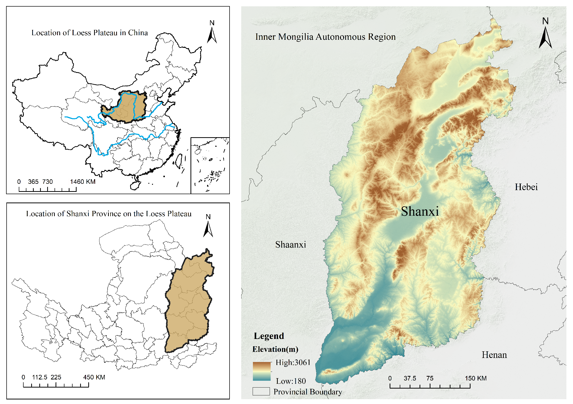
Figure 1. Study area: Shanxi Province in China. Note: The base map was sourced from the Standard Map (Approval No. GS (2019) 1822) [32], provided by the Ministry of Natural Resources of China, with no modifications to the original cartographic content.
Sustainability 17 09086 g001
Figure 2. Technical route diagram.
Sustainability 17 09086 g002
Figure 3. Dynamics of land use types, 1990–2022.
Sustainability 17 09086 g003
Figure 4. Land use transition Sankey bubble diagram, 1990–2022.
Sustainability 17 09086 g004
Figure 5. Temporal characteristics of land use carbon emissions from 1990 to 2022.
Sustainability 17 09086 g005
Figure 6. Spatial and structural distribution of land use carbon emissions in Shanxi Province from 1990 to 2022. (a) Carbon emissions and proportion by intensity class in 1990. (b) Same for 2000. (c) Same for 2010. (d) Same for 2022.
Sustainability 17 09086 g006
Figure 7. Spatial autocorrelation of carbon emissions in Shanxi Province in 1990, 2000, 2010, and 2022.
Sustainability 17 09086 g007
Figure 8. Land use carbon emission efficiency (LUCE) from 1990 to 2022, derived using the Stage 1 SBM-DEA model in Shanxi Province.
Sustainability 17 09086 g008
Figure 9. Land use carbon emission (LUCE) from 1990 to 2022, based on the Stage 3 SBM-DEA model in Shanxi Province.
Sustainability 17 09086 g009
Figure 10. Carbon emission efficiency scores of Shanxi cities under Stage 1 and Stage 3: (a) Stage 1 TE; (b) Stage 1 PTE; (c) Stage 1 SE; (d) Stage 3 TE; (e) Stage 3 PTE; (f) Stage 3 SE. Efficiency scores are dimensionless (–).
Sustainability 17 09086 g010
Figure 11. Robustness of feature importance rankings (bootstrap analysis: n = 500 ) for key drivers of land use carbon emissions.
Sustainability 17 09086 g011
Figure 12. SHAP interaction values for key global drivers of land use carbon emissions.
Sustainability 17 09086 g012
Table 1. Carbon emission coefficient recalibration scheme for Shanxi Province.
Land TypeCalibration ParameterShanxi ValueNational Value [33]Adjustment FactorMagnitude
Cultivated LandChemical Fertilizer Application100 kg·ha−185 kg·ha−1 α 1.18 +18%
Construction LandEnergy Consumption per Unit GDP0.5 tce·10 k CNY−10.4 tce·10 k CNY−1 β = 1.25 +25%
Forest LandNet Primary Productivity (NPP)200 kg·ha−1227 kg·ha−1 γ f 0.88 −12%
GrasslandNet Primary Productivity (NPP)150 kg·ha−1176 kg·ha−1 γ g 0.85 −15%
Note: The recalibrated coefficient for construction land is validated against the provincial-scale building carbon emission (BCE) findings in [35].
Table 2. Carbon emission coefficients for land use types in Shanxi Province.
TypeCultivatedForestGrasslandWaterUnusedConstruction
Value
(t · ha−1 · a−1)
0.422 0.644 0.021 0.253 0.00542.970
Table 3. Evaluation indicators of carbon emission efficiency.
CategorySpecific IndicatorIndicator DescriptionUnitData Source and Processing
Input variablesCapital stockFixed capital stockCNY 100 millionCalculated based on the perpetual inventory method; data from Shanxi Statistical Yearbook and local statistical yearbooks.
Labor forceYear-end employed population10,000 personsStatistical data from Shanxi Statistical Yearbook and local statistical yearbooks.
LandCarbon sources: construction land, cultivated land; Carbon sinks: forest land, grassland, water bodies, unused landhaLand use classification from the product of Huang Xin’s team (Wuhan University); city-level areas clipped in ArcGIS.
Output variablesDesirable outputRegional gross domestic productCNY 100 millionData from Shanxi Statistical Yearbook and local statistical yearbooks.
Undesirable outputTotal land use carbon emissions10,000 tDerived by summing county-level land use carbon emissions estimates.
Environment variablesUrbanization rateProportion of urban permanent residents to total populationData from Shanxi Statistical Yearbook and local statistical yearbooks.
Economic development levelPer capita GDPCNYData from Shanxi Statistical Yearbook and local statistical yearbooks.
Industrial structureShare of secondary industry value-added in RGDPData from Shanxi Statistical Yearbook and local statistical yearbooks.
Population densityTotal population divided by urban areaPersons/km2Population data from Shanxi Statistical Yearbook; land area derived from statistical yearbooks.
Green technology progress indexProportion of green patent grants to total patentsPatent data from the China National Intellectual Property Administration.
Government interventionRatio of local fiscal expenditure to RGDPLocal fiscal expenditure and GDP data from Shanxi Statistical Yearbook and local statistical yearbooks.
Table 4. Carbon emission driver indicator system.
Criterion LayerIndicator LayerVariable DefinitionUnit
Economic DevelopmentURProportion of urban permanent residents to total population
RGDPFinal output of productive activities by regional units within a given periodCNY 100 million
SICPercentage of secondary industry in industrial structure
Technological InnovationGTPIRatio of green patent grants to total patents
Land Use PatternsNDVIReflects surface vegetation coverage
Human ActivitiesPOPDPopulation per unit areaPersons/km2
POPSTotal permanent population10,000 persons
HFDDegree of human modification to land surfaces
Natural EnvironmentPAnnual average precipitationmm
TAnnual average temperature°C
Table 5. SFA regression results.
Environmental VariablesCapital StockLabor ForceLand Area
cons0.0016−0.0356−0.2515
(0.1215)(−0.7332)(−2.2447)
UR0.1056 ***0.2084 **0.3311
(3.3446)(2.2623)(1.3554)
GOV0.0214−0.05160.6164 ***
(1.1091)(−1.0935)(4.0618)
PGDP−0.1639 ***−0.1283 **−0.3113
(−4.7281)(−2.0378)(−2.0818)
GTPI−0.00590.0880 ***−0.0773
(−0.3890)(2.1377)(−0.7280)
POPD0.0233−0.2221 **−0.2300
(0.6705)(−2.2654)(−0.9772)
INS−0.00320.02650.177
(−0.2075)(0.5667)(1.4587)
σ 2 0.0094 **0.0041 **0.0393 *
(2.3624)(2.3624)(1.9756)
γ 0.9638 ***0.43160.5981
(5.7327)(1.9256)(2.3976)
Log-likelihood
function
101.4258 ***56.5474 ***17.7302 ***
(5.1431)(4.1546)(3.1842)
LR one-sided error
test values
29.4255 ***40.3694 ***19.4377 ***
(4.2631)(5.9847)(4.3412)
Notes: *, **, and *** denote statistical significance at 10%, 5%, and 1% levels, respectively. T-statistics are reported in parentheses.
Table 6. Period decomposition of efficiency changes by stage (1990–2022).
Efficiency MeasureStage1990–20002000–20102010–2022
TEStage 1+0.034+0.068+0.046
TEStage 3+0.040−0.071−0.264
PTEStage 1+0.082−0.083−0.080
PTEStage 3+0.019+0.039−0.010
SEStage 1−0.073+0.156+0.064
SEStage 3+0.021−0.120−0.272
Table 7. Robustness check for land variable specification.
Efficiency MeasureMean Change Δ Std. Dev.Spearman’s ρ
TE 0.326 + 0.029 0.957 ***
PTE 0.252 + 0.109 0.91 ***
SE 0.212 + 0.048 0.966 ***
Note: This table compares the primary model (land as inputs) against the robustness check model (land as environmental variables). Spearman’s ρ represents the average correlation of city rankings across the study period. *** p < 0.001 .
Table 8. Uncertainty in city-level efficiency scores (2022).
CityTE-p5TE-p50TE-p95SE-p5SE-p50SE-p95
Taiyuan0.5210.5630.6020.6320.7020.768
Datong0.4580.5020.5430.5540.6210.685
Yangquan0.6020.6480.6910.5870.6620.733
Changzhi0.4870.5310.5740.6120.6830.751
Jincheng0.5340.5770.6180.6630.7350.803
Shuozhou0.4230.4670.5100.5220.5900.656
Jinzhong0.4650.5090.5520.5780.6480.715
Yuncheng0.4410.4850.5270.5980.6680.736
Xinzhou0.3980.4420.4850.5010.5690.635
Linfen0.4520.4960.5390.5620.6310.698
Lvliang0.4110.4550.4980.5340.6020.668
Median IPR0.084 0.136
Note: p5, p50 (median), and p95 percentiles are derived from 1000 Monte Carlo iterations. IPR (Inter-Percentile Range) = p95 − p5. The median IPR across cities shows that SE is ∼62% more sensitive to emission coefficient uncertainty than TE.
Table 9. Spatial cross-validation performance metrics of the XGBoost model in Shanxi Province.
Fold R 2 RMSE
10.63510.570
20.8448.848
3 (Region 2)−0.05516.602
40.62811.840
50.69616.055
Average0.55012.783
Note: Fold 3 corresponds to Region 2, the area exhibiting a distinct socio-ecological profile.
Table 10. Comparison of Region 2 characteristics with overall study area averages.
FeatureOverall MeanRegion 2 MeanRelative DifferenceImplication
WSF15.7718.13+15.0%Elevated anthropogenic intensity
UR0.620.67+11.2%Higher urban density and energy use
T (°C)7.667.10 26.2 %Colder climate, increased heating demand
P (mm)549.04439.74 25.7 %Drier conditions, weaker natural sinks
NDVI0.420.31 35.7 %Lower vegetation cover, diminished ecological regulation
WSF represents the human footprint index, encompassing urban expansion, industrial activity, and infrastructure development.
Disclaimer/Publisher’s Note: The statements, opinions and data contained in all publications are solely those of the individual author(s) and contributor(s) and not of MDPI and/or the editor(s). MDPI and/or the editor(s) disclaim responsibility for any injury to people or property resulting from any ideas, methods, instructions or products referred to in the content.