Performance Improvement of a Standalone Hybrid Renewable Energy System Using a Bi-Level Predictive Optimization Technique

Abstract

A standalone hybrid renewable energy system (HRES) that combines different types of renewable energy sources and storages offers a sustainable energy solution by reducing reliance on fossil fuels and minimizing greenhouse gas emissions. In this paper, a standalone hybrid renewable energy system (HRES) involving wind turbines, photovoltaic (PV) modules, diesel generators (DG), and battery banks is proposed. For this purpose, it is necessary to size and run the proposed system for feeding a residential load satisfactorily. For two typical winter and summer weeks, weather historical data, including irradiance, temperature, wind speed, and load profiles, are used as input data. The overall optimization framework is formulated as a bi-level mixed-integer nonlinear programming (BMINLP) problem. The upper-level part represents the sizing sub-problem that is solved based on economic and environmental multi-objectives. The lower-level part represents the energy management strategy (EMS) sub-problem. The EMS task utilizes the model predictive control (MPC) approach to achieve optimal technoeconomic operational performance. By the definition of BMINLP, the EMS sub-problem is defined within the constraints of the sizing sub-problem. The MATLAB R2023a environment is employed to execute and extract the results of the entire problem. The global optimization solver “ga” is utilized to implement the upper sub-problem while the “intlinprg” solver solves the lower sub-problem. The evaluation metrics used in this study are the operating, maintenance, and investment costs, storage unit degradation, and the number of CO₂ emissions.

1. Introduction

Rising populations worldwide have increased energy demand, which has resulted in stresses on conventional energy resources in recent years. Thus, exacerbating these stresses necessitates greater resource consumption, which results in worsened environmental problems such as air pollution, increased greenhouse gases, and global warming. Globally, the tendency towards reliance on multi-source energy systems has begun due to the environmental concerns mentioned above. Attempts are being made to replace renewable energy sources with fossil fuels and to use cutting-edge technologies in energy storage systems such as batteries and hydrogen storage systems to start shifting towards carbon-free multi-source energy systems [1]. A hybrid renewable energy system (HRES) is a prominent example of a multi-source energy system. The term HRES is used to describe a system that comprises multiple energy sources, with at least one of them being renewable, combined by one or more energy storage systems. The term HRES is usually applied to both standalone and grid-connected systems [2].

An existing backup energy system is crucial in HRES; this is due to the nonhomogeneous distribution and unpredictable behavior of renewable resources, such as sun radiation and wind speed, which are constantly fluctuating. These systems act as a safety net for the HRES, which ensures continuity of energy supply in case of energy shortages [3]. Several sectors can benefit from HRESs. In remote areas, the expansion of these systems in remote areas increases the portion of people with electricity service and lessens their reliance on fossil fuels as an energy source [4]. The use of hybrid renewable energy systems in the manufacturing sector aids in reducing the high production cost associated with energy usage. Moreover, the energy produced by these systems can contribute to encountering load requirements for cooling or heating purposes [5]. Additionally, HRESs are further employed in water sectors for pumping irrigation water and powering desalination plants [6,7].

The current literature on HRESs is extensive and concentrates particularly on the sizing task [8,9,10,11,12,13,14,15,16,17]. Bahgaat [8] proposed an HRES comprising photovoltaic (PV) panels and wind turbines, diesel generators, and battery banks to feed a long-term evolution (LTE) mobile station installed at a far-off area in the 6th of October City, Egypt. The main objectives were to attain optimal technoeconomic performance of the suggested system by achieving the minimum levelized cost of energy (LCOE) and the maximum renewable energy fraction (REF). The hybrid optimization of multiple energy resources (HOMER) tool was utilized to configure and investigate four different configurations: only grid-off PV panels, PV panels and diesel generators, wind turbines alone, and grid-on PV panels. The results revealed that the best system schematic was the only grid-off PV panels based on economic and environmental criteria. The authors of [10] introduced a grid-off HRES configuring with wind turbines, PV panels, and diesel generators as energy sources in addition to either pumped thermal units or battery banks as storage subsystems. Using the MATLAB environment, a mixed-integer linear programming (MILP) solver was utilized for optimum sizing and energy flow scheduling. The proposed system was targeted to conquer minimum total annual cost, considering a demand response program. This program was established based on instantaneous renewable source accessibility with an active pricing economic model. Iqbal et al. [13] provided an HRES intended to power a microgrid system of a passenger vessel. Three system configurations were analyzed: (1) PV/wind/battery, (2) PV/wind/battery/diesel, and (3) PV/wind/fuel cell/battery. The system performance was evaluated based on techno-eco-environmental metrics, i.e., energy production, LCOE using net present value, and CO₂ emission. Furthermore, two battery technologies, lead acid battery (LAB) and lithium-ion battery (LIB), were utilized as storage units. The authors of [14] presented an HRES involving PV modules, diesel generators, and battery packs of a standalone HRES. Three distinct objectives were employed to size the proposed HRES optimally. These objectives were the loss of load probability, CO₂ emission amount, and the annualized cost of the system. The ε-constraint method was used to convert the multi-objective function to a single-objective function, which was implemented by an improved coyote optimization algorithm (ICOA). The proposed method was compared with the particle swarm optimization (PSO) approach and HOMER tool. The findings show that the suggested ICOA-based system outperforms the PSO-based and HOMER-based systems according to renewable contribution and CO₂ emissions indicators. To conclude this part, the studies were focused on using artificial intelligence methods and software tools to construct the HRES. On the contrary, some researchers have used conventional approaches to optimize the HRES, such as probabilistic [18], iterative [19], and analytical [20] approaches, because they are relatively straightforward and simple to execute [21].

More recent attention has been focused on the provision of EMS techniques [22,23,24,25,26,27,28,29,30,31]. For standalone HRESs, Kavadias et al. [3] proposed an adaptive and dynamic intelligent power management control (IPMC) considering the weather variations. The suggested approach was formulated using the fuzzy logic control (FLC) via MATLAB’s Simulink. Using the FLC ensured the balance between the power sources and accomplished the stability and security of the system operation. The simulation results were compared with real-time results obtained from a simulator called OPAL RT LAB. Nair and Sundari [25] introduced the gazelle optimization algorithm (GOA) to optimize the energy operation within a 24-h control horizon. Moreover, a spiking neural network (SNN) was employed to forecast energy demand using historical data and external factors. The hybrid GOA–SSN approach considered the consumers’ behavior affected by electricity prices to determine the ideal intervals, within the day, for offering them lower prices. Generally, the suggested method is intended to reduce human involvement and leverage advanced bi-directional communication. The authors of [27] established a method linking model predictive control (MPC) with dynamic programming (DP) for sequential operation scheduling of a grid-on PV and a battery HRES. Three distinguished strategies were introduced: the economic optimization strategy, the grid-power optimization strategy, and the maximizing self-consumption strategy. These strategies were executed experimentally and the associated results were compared with the simulated results. By using a real-date load profile, the authors of [28] performed an optimal EMS for a microgrid using the economic model predictive control (EMPC) approach. To run the proposed microgrid, the EMS problem was expressed as a mixed-integer nonlinear programming (MINLP) problem.

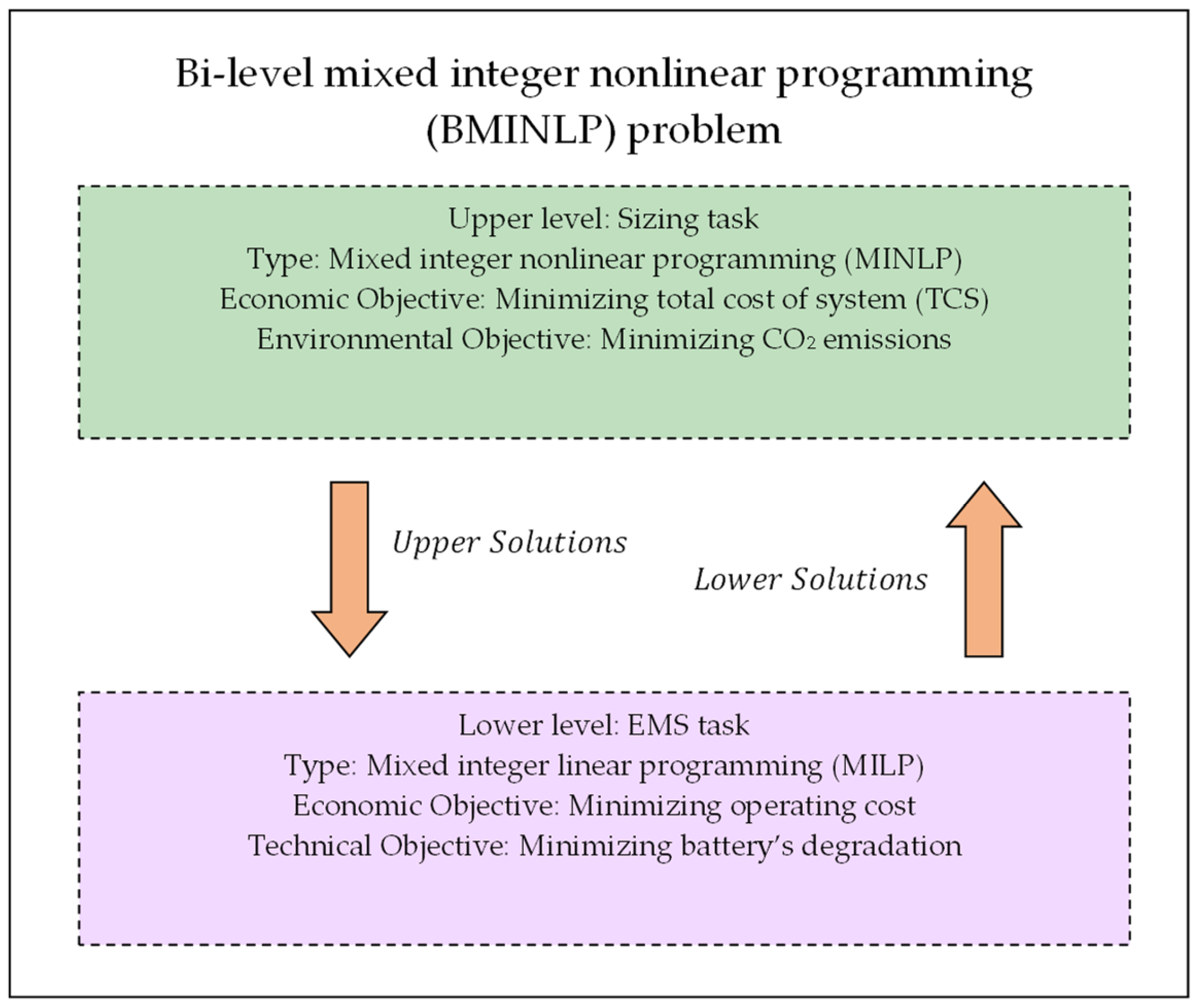
The authors of [32,33,34] employed a bi-level optimization technique that contains two levels, each comprising an independent optimization task in conjunction with the objective, variables, constraints, and their mathematical nature. The main feature of this method is that the lower task is nested within the constraints of the upper task. In view of that, the sizing optimization sub-problem can be defined within the upper task. It is formulated to configure the system optimally based on achieving the best eco-environmental performance. The sizing sub-problem involves four integer variables, representing the number of units associated with wind turbines, PV modules, diesel generators, and batteries. The lower task expresses the EMS sub-problem, which targets managing the power flows and the operational status storage components. This sub-problem is framed based on the MPC approach with MILP formulation. The upper variables are considered fixed parameters during the lower task-solving process and vice versa. Generally, the entire problem is classified as a bi-level mixed-integer nonlinear programming (BMINLP) optimization problem carried out using the MATLAB program [35]. Figure 1 illustrates the basic principle behind the suggested bi-level optimization technique. The following are the primary contributions provided by the present study:

• A BMINLP problem-solving approach is established by applying a best-practice approach to configure a standalone HRES assimilated by an EMS.
• An eco-environmental multi-objective approach is presented for implementing the higher-level task (sizing), while another distinguished technoeconomic multi-objective approach defines the lower-level task (EMS).
• Applying a robust EMS-based method (MPC) to improve HRES operation.

The remaining part of the paper proceeds as follows: Section 2 demonstrates the suggested system modeling. The technique, as described in Section 3, dives into great detail about the formation of the size and EMS tasks. Section 4 discusses and displays the relevant outcomes. The conclusion is eventually provided in Section 5.

2. System Modeling

This research intends to configure a standalone HRES feeding a residential load. The suggested HRES encompasses PV panels and wind turbines as the primary energy sources, with backup sources represented by the diesel generators. The battery banks play the role of the energy storage system (ESS). Figure 2 illustrates the single-line diagram of the suggested HRES.

The following subsections represent the mathematical modeling for each component.

2.1. Photovoltaic Model

The nonlinear voltage–current characteristic can be mathematically expressed by (1) [17].

$$I_{pv}=\left(N_p{I}_{ph}-N_p{I}_{rs}\right)\times \left[\mathit{exp}\left({\displaystyle \frac{q\left(V_{pv}+I_{pv}{R}_s\right)}{N_s{A}_{c}K{T}_c}}\right)-1\right]$$

(1)

Both $I_{ph}$ and $I_{rs}$ represent the generated current for a specific irradiance ($\lambda$) and the reverse saturation current, respectively. The other symbols ($A_c,K,R_s,q,N_s,N_p, \mathrm{a}\mathrm{n}\mathrm{d} T_c$) express the p–n junction constant, Boltzmann constant, intrinsic cell resistance, electron charge, serially connected cells per string, number of parallel strings, and cell temperature in kelvin, correspondingly. The equations below illustrate how $I_{ph}$ and $I_{rs}$ are affected by the irradiance ($\lambda$) and surrounding temperature ($T_a$) in kelvin.

$$I_{ph}=\left(I_{sc}+K_l\left(T_c-T_r\right)\right)\times {\displaystyle \frac{\lambda }{1000}}$$

(2)

$$I_{rs}=I_{or}{\left({\displaystyle \frac{T_c}{T_r}}\right)}^3\times exp\left({\displaystyle \frac{{qE}_g\left(\frac{1}{T_r}-\frac{1}{T_c}\right)}{K{A}_c}}\right)$$

(3)

$$T_c=T_a+\left({\displaystyle \frac{NOCT-20}{800}}\right)\times \lambda$$

(4)

$I_{sc}$ is the cell short-circuit current at a reference temperature ($T_r$) and irradiance, and $K_l$ is the temperature coefficient of the short-circuit current. $E_g$ denotes the band-gap energy of the cell semiconductor, whereas $I_{or}$ represents the reverse saturation current represented by the reference temperature. $NOCT$ stands for the nominal operating cell temperature in Celsius. Therefore, the total PV output power, supplied to the DC bus, can be expressed by the following formula:

$$P_{pv}={\eta }_{pv}·N_{pv}·P_{pv,m}$$

(5)

where ${\eta }_{pv}$ is the efficiency of the PV converter, while $N_{pv}$ refers to the total number of modules. The maximum available power per module is denoted by $P_{pv,m}$. Noteworthily, the technical description of the utilized PV module is listed in

Table A1. Technical description of PV module [36].

Brand	Sunmodule SW 240 Poly
Electron charge ($q$)	$1.6\times {10}^{-19} \mathrm{C}$
Constant of p–n junction ($A_c$)	$1.6$
Boltzmann constant ($K$)	$1.3805\times {10}^{-23} \mathrm{N}\mathrm{m}/\mathrm{K}$
Short-circuit coefficient ($K_l$)	$5.532\times {10}^{-3} \mathrm{A}/\mathrm{K}$
Reverse saturation current ($I_{or}$)	$1.0647\times {10}^{-6} \mathrm{A}$
Reference temperature ($T_r$)	$303 \mathrm{K}$
Band-gap energy ($E_g$)	$1.1 \mathrm{V}$
Short-circuit current ($I_{sc}$)	$8.51 \mathrm{A}$
Intrinsic cell resistance ($R_s$)	$0.01 \mathsf{\Omega }$
Nominal operating cell temperature ($NOCT$)	$46 °\mathrm{C}$
Parallel strings ($N_p$)	$1$
Serial cells per string ($N_s$)	$60$
Number of panels per module	$4$
Rated power of PV module unit ($P_{pv,r}$)	$1 \mathrm{k}\mathrm{W}$
Capital cost (${CC}_{pv}$) (USD)	$7000$
Lifetime (${LT}_{pv}$)	$20 \mathrm{y}\mathrm{e}\mathrm{a}\mathrm{r}\mathrm{s}$
Maintenance cost ($C_{om,pv}$) (USD)	$20/\mathrm{y}\mathrm{e}\mathrm{a}\mathrm{r}$
PV converter efficiency (${\eta }_{pv}$)	$0.95$

(Appendix A) [36].

2.2. Wind Turbine Model

The power–speed characteristic of the nominated wind turbine can be expressed as follows [23]:

$$P_{w,t}=\left\{\begin{array}{c}{P}_{w,r}{\left({\displaystyle \frac{v_w-v_{in}}{v_r-v_{in}}}\right)}^3,v_{in}\le v_w\le v_r\\ P_{w,r} , v_r\le v_w\le v_o \\ 0, otherwise\end{array}\right.$$

(6)

where $P_{w,r}$ and $v_r$ are the rated power and speed, while $v_{in}$ and $v_o$ refer to the nominated cut-in and cut-out speeds. Indeed, the wind speed varies with respect to the altitude. Thus, the measured wind speeds ($v_{w,m}$) at ${(H}_m)$ can be extrapolated to the hub altitude ($H_{hub})$, which is normally calculated using the following formula:

$$v_w=v_{w,m}{\left({\displaystyle \frac{H_{hub}}{H_m}}\right)}^{\alpha }$$

(7)

Depending on the topology of the surface, the wind shear coefficient ($\alpha$) is picked to be 0.15 [37].

As a result, the total extracted power from ($N_w$) wind turbine unit, delivered to the DC bus, is expressed as follows:

$$P_w={\eta }_w·N_w·P_{w,t}$$

(8)

Noteworthily, the technical description of the utilized wind turbine model is listed in

Table A2. Technical description of wind turbine model [38].

Brand	Eocycle EO20
Rated power ($P_{w,r}$)	$\mathrm{20,000} \mathrm{W}$
Cut-in wind speed ($v_{in}$)	$2.75 \mathrm{m}/\mathrm{s}$
Rated wind speed ($v_r$)	$7.5 \mathrm{m}/\mathrm{s}$
Cut-out wind speed ($v_o$)	$20 \mathrm{m}/\mathrm{s}$
Hub height ($H_{hub}$)	$36 \mathrm{m}$
Reference height ($H_m$)	$10 \mathrm{m}$
Wind shear exponent ($\alpha$)	$0.25$
Capital cost (${CC}_w$) (USD)	$\mathrm{38,745}$
Lifetime (${LT}_w$)	$20 \mathrm{y}\mathrm{e}\mathrm{a}\mathrm{r}\mathrm{s}$
Maintenance cost ($C_{om,w}$) (USD)	$3\% {CC}_w/\mathrm{y}\mathrm{e}\mathrm{a}\mathrm{r}$
Wind converter efficiency (${\eta }_{w,conv}$)	$0.90$

[38].

2.3. Diesel Generator

Generally, several types of generators can be used in the HRES: internal combustion engine generators (e.g., diesel generators), fuel cell generators, and micro-turbines [7]. In this research study, only the diesel generators are used in the HRES under test. The fuel consumption in liters for ($N_{dg}$) diesel generators can be expressed as follows [32]:

$$K_{fuel}\left(t\right)=N_{dg}·\left(a·P_{dg}\left(t\right)+b·P_{dg}^{nom}\right)·∆t$$

(9)

where $P_{dg}$ and $P_{dg}^{nom}$ are the output and nominal power of DG in kW, and a and b are constant depending on the quality of DG in ($\mathrm{L}/\mathrm{k}\mathrm{W}\mathrm{h}$). The technical description of the used diesel generator model is summarized in

Table A3. Technical description of diesel generator model [39].

Nominal power (${\mathit{P}}_{\mathit{d}\mathit{g}}^{\mathit{n}\mathit{o}\mathit{m}}$)	$2000 \mathrm{W}$
Diesel generator constant ($a$)	$0.246 \mathrm{L}/\mathrm{k}\mathrm{W}\mathrm{h}$
Diesel generator constant ($b$)	$0.08145 \mathrm{L}/\mathrm{k}\mathrm{W}\mathrm{h}$
Fuel price (${Pr}_{fuel}$) (USD)	$1.06/\mathrm{L}$
Emission factor ($E_f$)	$2.6 \mathrm{k}\mathrm{g}/\mathrm{L}$
Diesel fuel’s unit conversion factor ($\mathrm{S}$)	$0.8$
Lifespan (${LT}_{dg}$)	$25 \mathrm{y}\mathrm{e}\mathrm{a}\mathrm{r}\mathrm{s}$
Capital cost ($C_{dg}$) (USD)	$1514$
Maintenance cost (${{CC}_m}_{dg}$) (USD)	$0.17/\mathrm{h}$
Diesel generator converter efficiency (${\eta }_{dg}$)	$0.95$

[39].

2.4. Battery

The linear model using the following equation can express the battery’s state of charge (${SoC}_b$) [24]:

$${SoC}_b\left(k+1\right)={SoC}_b\left(k\right)+{\displaystyle \frac{P_{b_{ch}}-P_{b_{disch}}}{N_b·E_{b,u}}}·∆t$$

(10)

where $P_{b_{ch}} \mathrm{and} P_{b_{disch}}$ denote the battery’s charging and discharging power, respectively. $N_b$ represents the number of battery units, whereas $E_{b,u}$ is the rated energy capacity per unit. The other technical specifications of the used battery model are shown in

Table A4. Technical description of battery model [40].

Energy capacity (${\mathit{E}}_{\mathit{b},\mathit{u}}$)	$1190 \mathrm{Wh}$
Maximum discharge power ($P_{b_{disch}}$)	$1190 \mathrm{W}$
Maximum charge power ($P_{b_{ch}}$)	$1190 \mathrm{W}$
Maximum state of charge (${SoC}_b^{max}$)	$0.9$
Minimum state of charge (${SoC}_b^{min}$)	$0.4$
Discharging factor ($B$)	1.165
Capital cost (${CC}_b$) (USD)	$2000$
Equivalent full cycles ($N_{c_b}$)	$1500$
Maintenance cost ($C_{{om}_b}$) (USD)	$5\% {\mathrm{C}\mathrm{C}}_{\mathrm{b}}/\mathrm{y}\mathrm{e}\mathrm{a}\mathrm{r}$
Battery bi-directional converter (${\eta }_b$)	$0.95$

[40].

2.5. Load Shedding and Generation Curtailment

When there is a substantial demand and the total generation of the system, including renewable generation, DG, and battery, fail to satisfy it, a shortage of the power supplied to the load will occur. In this case, the issue can be resolved by defining a new term: load shedding. Hence, the system is invoked to reduce the demand by this value. On the contrary, when there is excess generation and the battery is saturated, the system tackles this issue by decreasing the generation with a certain value, i.e., the curtailed power. Consequently, the following equations can always satisfy the power balance at the DC bus:

$$P_{pv}+P_w+P_{dg}+P_{b_{disch}}+P_{ls}={\displaystyle \frac{P_{Load}}{{\eta }_{inv}}}+P_{b_{ch}}+P_{rc}$$

(11)

where $P_{Load}$ symbolizes the load power and ${\eta }_{inv}$ represents the efficiency of the attached inverter. Moreover, $P_{ls}$ and $P_{rc}$ refer to the new terms, load shedding and generation curtailment powers, respectively.

3. Methodology

The current study utilizes the bi-level technique to formulate the overall optimization problem. The bi-level optimization technique involves solving two sub-problems with unique variables, constraints, and objectives. The lower-level sub-problem is framed as part of the upper-level sub-problem’s constraints. Generally, the following can mathematically state the bi-level problem [41]:

$$\begin{gathered} \underset{\mathit{x}}{Min }F\left(x,y\right) \\ \mathrm{Subject} \mathrm{to:} \\ h\left(x,y\right)\le 0 \\ y\in \arg \underset{\mathit{y}}{Min} G\left(x,y\right) \\ \mathrm{Subject} \mathrm{to:} \\ k\left(x,y\right)\le 0 \end{gathered}$$

(12)

where $F\left(x,y\right)$ refers to an objective function representing the upper sub-problem, whereas $G\left(x,y\right)$ is the objective function associated with the lower sub-problem. $h\left(x,y\right)$ denotes upper-level constraints, while the lower-level constraints are represented by $k\left(x,y\right)$.

In this investigation, each level’s sub-problem is established with a multi-objective function. Nevertheless, the problem can be simplified by converting the multi-objective function (MOF) to a single-objective function using the normalization approach [42]. Consequently, this technique avoids the prioritization of one single-objective function over the others, as well as reduces the overall consumed time that is required to solve the problem. Mathematically, the normalization process, in conjugated with conventional weighted aggregation, can be expressed as follows [42]:

$$MOF=\sum _{i=1}^s{w}_i·{\displaystyle \frac{f_i}{f_{max}}}$$

(13)

where $w_i$ denotes the nonnegative weight. $f_i$ and $f_{max}$ are the single-objective function and its maximum value. Each sub-problem will be addressed in the following subsections.

3.1. Formulation of Lower-Level Sub-Problem

The lower-level sub-problem characterizes the EMS task within the HRES. Therefore, it aims to operate and manage power flow between the system’s components effectively. In detail, the lower sub-problem is framed as MILP optimization to achieve minimum operating cost and minimum battery degradation. The corresponding decision variables are power flows associated with the battery banks, diesel generators, load shedding, and generation curtailment, as well as the operational statuses related to charging and discharging of the battery. The EMS sub-problem is solved using the MPC technique, which is extensively addressed in [17]. The mathematical formulation of the EMS sub-problem is given by the following set of equations [43,44]:

$$\begin{array}{c}\underset{X\left(i|k\right)}{\min }{\displaystyle \sum _{i=0}^{H_p-1}}{J}_{EMS}\left(x\left(i|k\right)\right)={\displaystyle \frac{w_1}{{J_{op}}_{max}}}{\displaystyle \sum _{i=0}^{H_p-1}}{\displaystyle \sum _{j\in \mathcal{L}}}{J}_{o{p}_j}\left(x\left(i\right|k)\right)+{\displaystyle \frac{w_2}{{J_D}_{max}}}{\displaystyle \sum _{i=0}^{H_p-1}}{J}_D\left(x\left(i|k\right)\right)\\ \hspace{1em}\hspace{1em}\hspace{1em}\hspace{1em} \mathrm{subject} \mathrm{to:}\end{array}$$

(14a)

$$J_{{op}_b}\left(i|k\right)={\displaystyle \frac{{CC}_b·∆t}{2N_{c_b}{E}_{b,u}}}·\left(P_{b_{ch}}\left(i|k\right)+P_{b_{disch}}\left(i|k\right)\right)$$

(14b)

$$J_{{op}_{dg}}\left(i|k\right)={Pr}_{fuel}·\left(a·P_{dg}\left(i|k\right)+b·P_{dg}^{nom}\right)·∆t$$

(14c)

$$J_{{op}_{ls}}\left(i|k\right)=C_{ls}·P_{ls}\left(i|k\right)·∆t$$

(14d)

$$J_{{op}_{rc}}\left(i|k\right)=C_{rc}·P_{rc}\left(i|k\right)·∆t$$

(14e)

$$J_{D_b}\left(i|k\right)={\displaystyle \frac{0.5·∆t}{N_{c_b}{E}_{b,u}}}·\left(P_{b_{ch}}\left(i|k\right)+{\displaystyle \frac{P_{b_{disch}}\left(i|k\right)}{B}}\right)$$

(14f)

$${\eta }_{pv}·N_{pv}·P_{pv}\left(i|k\right)+{\eta }_w·N_w·P_w\left(i|k\right)+P_{dg}\left(i|k\right)+P_{b_{disch}}\left(i|k\right)+P_{ls}\left(i|k\right)={\displaystyle \frac{P_{Load}\left(i|k\right)}{{\eta }_{inv}}}+P_{b_{ch}}\left(i|k\right)+P_{rc}\left(i|k\right)+P_{loss}\left(i|k\right)$$

(14g)

$$P_{loss}\left(i|k\right)=2\%\times \left({\eta }_{pv}·N_{pv}·P_{pv}\left(i|k\right)+{\eta }_w·N_w·P_w\left(i|k\right)\right)$$

(14h)

$${SoC}_b\left(i+1|k\right)={SoC}_b\left(i|k\right)+{\displaystyle \frac{P_{b_{ch}}\left(i|k\right)-P_{b_{disch}}\left(i|k\right)}{N_b{E}_{b,u}}}·∆t$$

(14i)

$${SoC}_b^{min}\le {SoC}_b\left(i|k\right)\le {SoC}_b^{max}$$

(14j)

$$0\le P_{b_{ch}}\left(i|k\right)\le {\delta }_{b_{ch}}\left(i|k\right)·N_b·{\displaystyle \frac{P_{b_{ch}}^{max}}{{\eta }_b}}$$

(14k)

$$0\le P_{b_{disch}}\left(i|k\right)\le {\delta }_{b_{disch}}\left(i|k\right)·{\eta }_b·N_b·P_{b_{disch}}^{max}$$

(14l)

$$0\le P_{dg}\left(i|k\right)\le {\eta }_{dg}·N_{dg}·P_{dg}^{max}$$

(14m)

$$0\le P_{rc}\left(i|k\right)\le {\eta }_{pv}·N_{pv}·P_{pv}\left(i|k\right)+{\eta }_w·N_w·P_w\left(i|k\right)$$

(14n)

$$0\le P_{ls}\left(i|k\right)\le {\displaystyle \frac{P_{Load}\left(i|k\right)}{{\eta }_{inv}}}$$

(14o)

$${\delta }_{b_{disch}}\left(i|k\right)-{\delta }_{b_{ch}}\left(i|k\right)\le 1$$

(14p)

With $x\left(i|k\right)=[P_{b_{ch}}\left(i|k\right),P_{b_{disch}}\left(i|k\right),P_{dg}\left(i|k\right),P_{ls}\left(i|k\right),P_{rc}\left(i|k\right),{\delta }_{b_{ch}}\left(i|k\right),{\delta }_{b_{disch}}\left(i|k\right)]$ and $\mathcal{L}=[b,dg,ls,rc]$, where $J_{{op}_b},J_{{op}_{dg}},J_{{op}_{ls}} \mathrm{and} J_{{op}_{rc}}$ refer to operating costs corresponding to the battery banks, diesel generators, load shedding, and generation curtailment.$H_p$ represents the prediction horizon. The degradation of the battery is expressed by $J_{D_b}$. ${CC}_b$ and $B$ denote the capital cost and the discharge factor of the battery. The notation $\left(i\right|k)$ represents the predicted future value for the instant $(i+k)$ for a given actual instant $k$. According to the EMPC approach, the remaining terms are discarded $(i=\left[1 : H_p-1\right])$, allowing the first term of solution $u\left(0\right|k)$ to be taken into account and applied to the size problem. Likewise, the progression is applied at each instant through the simulation period $k=1 : Ns$. ${Pr}_{fuel}$ is the fuel price in USD/L. $C_{ls}$ and $C_{rc}$ are energy unit costs in USD/kWh associated with load shedding and generation curtailment, which are selected to be 5.6 USD/kWh [45]. ${\eta }_b,{\eta }_{dg},{\eta }_{pv},{\eta }_w, \mathrm{and} {\eta }_{inv}$ are the converters’ efficiencies attached to the battery, diesel generator, PV, wind turbine, and load, respectively. The number of units relating to battery, diesel generator, PV, and wind turbine are $N_b,N,N_{pv}, \mathrm{and} N_w$.

3.2. Formulation of Upper-Level Sub-Problem

The upper-level sub-problem describes the sizing task in the HRES. Consequently, it aims to efficiently configure and design the suggested system based on eco-environmental objectives. Specifically, the upper sub-problem is constructed as MINLP optimization to accomplish two objective functions: minimizing the total cost of the system ($J_{TCS}$) and minimizing the CO₂ emissions ($J_{Emission}$). The corresponding decision variables are the number of units for each element in the system: batteries, diesel generators, PV modules, and wind turbines. The inclusive mathematical formulation of the sizing sub-problem, embedded within the EMS sub-problem, is expressed as follows [17,39]:

$$\begin{array}{c}\underset{N}{\mathrm{m}\mathrm{i}\mathrm{n}}\sum J_{sizing}=\frac{W_1}{{J_{TCS}}_{max}}·\sum _{j\in \mathcal{M}}{J}_{TCS}\left(N\right)+\frac{W_2}{{\displaystyle {J_{Emission}}_{max}}}·\sum J_{Emission}\left(N\right)\\ \mathrm{subject} \mathrm{to} \mathrm{the} \mathrm{following:}\hfill \end{array}$$

(15a)

$$J_{TCS}=J_{inv}+J_{omf}+J_{op}$$

(15b)

$$J_{inv}={\displaystyle \frac{1}{{LT}_s}}\sum _{j\in \mathcal{M}}{N}_j{CC}_j$$

(15c)

$$J_{omf}=\sum _{j\in \mathcal{M}}{N}_j{C}_{{om}_j}$$

(15d)

$$\forall k=\left[0:N_s-1\right]\left\{\begin{array}{c}lower level sub\text{-}problem \\ {SoC}_b^{\ast }\left(0|k+1\right)={SoC}_b^{\ast }\left(0|k\right)+{\displaystyle \frac{P_{b_{ch}}\left(i|k\right)-P_{b_{disch}}\left(i|k\right)}{N_b{E}_{b,u}}}∆t \\ J_{{op}_j}\left(k\right)=J_{{op}_j}\left(0|k\right) \end{array}\right.$$

(15e)

$$J_{\mathit{op}}=\sum _{k=0}^{N_s-1}{J}_{{op}_j}\left(k\right)$$

(15f)

$$J_{\mathit{Emission}}=N_{dg}·E_f·\mathrm{S}·\sum _{k=1}^{N_s}\left(a·P_{dg}\left(0|k\right)+b·P_{dg}^{nom}\right)·∆t$$

(15g)

$$N_j^{min}\le N_j\le N_j^{max}$$

(15h)

with $\mathcal{M}=\left\{b,dg,pv,w\right\}$, in Equations ($15\mathrm{e}) \mathrm{a}\mathrm{n}\mathrm{d} (15\mathrm{f}$) $j\in \left\{b,dg,ls,rc,loss\right\}$, and in Equation ($15\mathrm{h}$) $j\in \left\{b,dg,pv,w\right\}$.

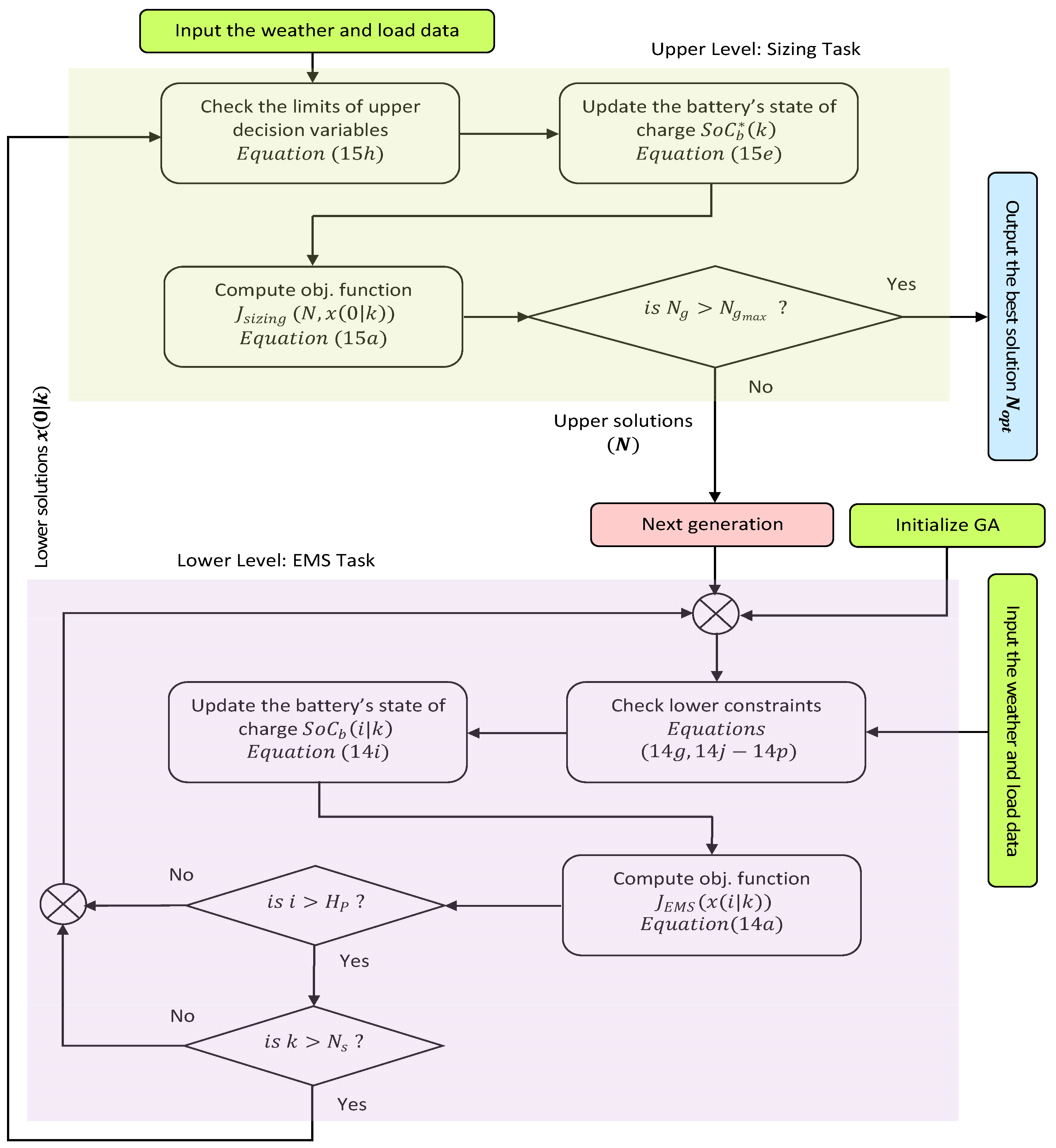
Here, $J_{inv}, J_{omf}, \mathrm{and} J_{op}$ represent the investment cost, fixed operation and maintenance cost, and the operating cost depending on EMS. ${CC}_j \mathrm{and} C_{{om}_j}$ are the capital and maintenance costs. ${LT}_s$ denotes the lifespan of the HRES. For diesel generators, $E_f$ is the emission factor, while $\mathrm{S}$ is the diesel fuel’s unit conversion factor. Figure 3 illustrates the solving procedure of both sub-problems as a bi-level optimization problem.

4. Results and Discussion

4.1. Input Data

The study is executed using the weekly weather-related and load datasets that are illustrated in Figure 4, Figure 5, Figure 6 and Figure 7. These datasets represent two distinct weeks, i.e., winter and summer weeks, during the year 2023 obtained from the open-access dataset [46]. The datasets are collected for a rural town located in the south of Jordan called Udhruh, which is shown in Figure 8. The load data characterize a benchmark residential building attained from an open database, the so-called OpenEI [47]. The description of the residential building is summarized in

Table A5. Technical description of load [47,48].

Type	Single-Family Detached House
Floor area	$355 {\mathrm{m}}^2$
Number of floors	$2$
Space heating method	Natural gas
Water heating method	Electric
Availability of air conditioning	Yes
Climate zone	Hot–humid
Maximum winter load	$\mathrm{28,999.5} \mathrm{W}$
Minimum winter load	$2828.9 \mathrm{W}$
Maximum summer load	$\mathrm{15,761.2} \mathrm{W}$
Minimum summer load	$3686.7 \mathrm{W}$
Load inverter efficiency (${\eta }_{inv}$)	$0.95$

[48]. The chosen weeks and related average values of the climatic and load data are revealed in

Table 1. The selected periods and related average statistics.

Week Sample	Winter	Summer
Period	1–7 February 2023	15–21 June 2023
Irradiance ($\mathrm{W}/{\mathrm{m}}^2$)	65.7	160.0
Wind Speed * ($\mathrm{m}/\mathrm{s}$)	8.9	6.0
Temperature ** ($\mathrm{K}$)	277.5	294.9
Load ($\mathrm{k}\mathrm{W}$)	15.1	9.1

* Wind speed is calculated at 36 m, i.e., hub height (wind shear exponent was taken as 0.15). ** Temperature is measured at 2 m height.

.

4.2. Problem Settings

In this investigation, the MATLAB environment is employed to run the BMINLP optimization problem and achieve the optimal solution. Accordingly, each level (sub-problem) entails a different solver based on the nature of the problem. MATLAB’s solver “intlinprg” is utilized to solve the optimization problem of the MILP type, which is the lower-level (EMS) sub-problem. This EMS is designed to run over the simulation period ($N_s$), which is 168 h. The prediction horizon ($H_P$) is set at six hours. This value was selected based on trial-and-error practices to achieve the best performance metrics. On the other hand, MATLAB’s solver “ga” is employed to implement the higher-level (sizing) sub-problem with the following settings: 5 generations ($N_g$) and 30 individuals in the population ($p$).

Table 2. The parameters of each sub-problem.

EMS Parameters
Problem type	Mixed-integer nonlinear programming (MINLP)
Solver	“ga” solver
Simulation period ($N_s$)	168 h
Prediction horizon ($H_P$)	6 h
Lower objectives’ weights ($w_1, w_2$)	0.5
Step time ($\mathsf{\Delta }\mathrm{t}$)	1 h
${\gamma }_{ls}$	1
${\gamma }_{rc,dg}$	2
${\gamma }_{bch,bdisch}$	0.1
Sizing Parameters
Problem type	Mixed-integer linear programming (MILP)
Solver	“intlinprog” solver
Population size ($p$)	30
Maximum number of generations ($N_g$)	5
Upper objectives’ weights ($W_1, W_2$)	0.5

lists all of the problem’s parameters.

4.3. Optimal Sizing

Table 3. Optimal sizing for proposed HRES.

Component	No. of Units
	Winter	Summer
PV module	14	7
Wind turbine	1	1
Battery	64	31
Diesel generator	14	8

presents the number of optimal units for each component constructing the proposed HRES across winter and summer periods. It can be observed from the table that the optimal system’s size based on winter operation is significantly larger than that resulting from summer operation.

The technical, economic, and environmental performance metrics are reported in

Table 4. Performance metrics of the proposed HRES.

	Winter	Summer
Battery degradation	0.003783	0.002603
Battery operating cost (USD)	8.1	5.3
Load shedding operating cost (USD)	0.0	0.0
Losses operating cost (USD)	4.7	2.7
DG operating cost (USD)	383.5	256.5
Operating cost (based on $N_s$) (USD)	396.3	264.5
Operating cost (scaled to one year) (USD)	20,664.2	13,791.8
Investment cost per year (USD)	14,297.1	8092.9
Fixed operation and maintenance cost per year (USD)	8094.6	4562.8
Total system cost (USD)	43,055.9	26,447.5
Emission (based on $N_s$)	1585.79 kg	958.10 kg

. From this table, it can be seen that the battery’s degradation value recorded in winter (0.0038) is greater than the summer-related value (0.0026). On the other side, the system costs USD 396.3 during the winter period, whereas it only costs USD 264.5 for the summer week’s operation. In more detail, the diesel generator makes the major contribution during both periods, with at least 96% of the overall cost. Interestingly, there is no load-shedding cost for the system in both weeks. A possible justification for this behavior of the system is that the diesel generator compensates for the shortage of the power supplied to the load continuously. Furthermore, the maximum investment and fixed operation and maintenance costs are attained in the winter period with USD 14,297.1 and USD 8094.6, respectively. These values are approximately twice the summer values (USD 8092.9 and USD 4562.8). Consequently, all of the above discussion is reflected in the total system costs, with USD 43,055.9 for winter and USD 26,447.5 for summer. From an environmental aspect, the diesel generator emits 1585.79 kg of CO₂, which is a considerably substantial amount compared to the summer value (958.10 kg).

The power profiles for both winter and summer weeks are shown in Figure 9 and Figure 10. A closer inspection of the figures demonstrates two scenarios of operation. These scenarios shed light on the management strategy followed to realize optimum operation.

In the first scenario, the load is greater than the renewable generation; therefore, the supplied power is deficient to the load. Initially, the EMS allows the DG to operate for compensating the power shortage, observing the sub-intervals of 120–150 h in the summer week of Figure 10. After that, when the DG reaches its maximum limits, the battery is permitted to intervene to cover the residual amount of power lack, observing the sub-intervals 50–60 h in winter week of Figure 9.

In the second scenario, the renewable generation is more than the load demand. In this case, the EMS is mainly invoked to curtail the generated power by the surplus power value, observing the sub-intervals 135–165 h in the winter week of Figure 9. In a few sub-intervals, the battery is allowed to charge the excess power unless the state of charge restrictions prevent its operation, observing the sub-intervals 80–90 h in the winter week of Figure 9. Figure 11 and Figure 12 illustrate the generated and demanded power distribution share for both winter and summer weeks. It is clear from these figures that the generated power by the wind turbine has the biggest amount, with around 50%, followed by the power produced by the DG, with nearly 45%, through both periods. In contrast, the other generative components (PV and battery discharging) do not produce more than 5% of the overall generated power. On the other hand, the power consumed by the load outperforms the other demanded components, with no less than 85% of the total power. Remarkably, the percentage values of the curtailed power are approximately 10% for winter and 13% for summer. On the contrary, the total percentage of power required in charging the battery through the period does not exceed 1% of the overall demanded power. To sum up, these findings confirm the EMS priority in operating the DG and battery.

A closer inspection of the results suggests some implications. Most significantly, the winter period had a significantly higher number of units than the summer period. This was due to the higher load requirement during the winter week. Moreover, this was reflected in the overall system cost and the number of CO₂ emissions. Compared to the summer period, the total system cost of winter was 63% greater, and the CO₂ emissions from operating the diesel generator were 65% higher. Additionally, the findings indicate that the EMS prioritizes operating the diesel generator ahead of turning on batteries, or implementing load-shedding steps in the scenario of a load shortage. This might be interpreted by stating that the operating cost required to produce one energy unit by the DG is significantly lower than the battery cost or the load-shedding cost. In detail, the diesel generator costs around USD 0.000173; however, the battery costs USD 0.000561. The operational cost required to shed one watt-hour is USD 0.0056, which is significantly higher than prior numbers.

4.4. Comparison with Nonoptimization Method

In order to highlight the impact of the proposed optimization method in this research study over the nonoptimization procedure, the system was tested during two distinct periods—a winter week and a summer week—and the results from both periods were compared. To support our claim, we propose an approach that determines the system size through simple and straightforward calculations (nonoptimization procedure). While the optimized algorithmic method focuses on identifying the optimal size based on minimizing total costs and CO₂ emissions, this simplified method aims to determine the number of units for each component solely based on meeting the maximum load demand. In detail, the proposed method can be summarized as follows:

• The minimum number of units required for each component to meet the maximum load is

  $$Component’s No. of units={\displaystyle \frac{Maximum Load}{Rated Capacity}}\times Safety Factor$$
• The components considered in this approach include PV panels, wind turbines, diesel generators, and batteries. A safety factor of 1.02, representing a 2% safety margin, is applied to ensure reliability in meeting the maximum load demand.
• The resulting system size was utilized to perform the energy management system (EMS) task, evaluate the system’s performance metrics, and present the findings in

  Table 5. Comparison between performance metrics of the proposed HRES based on optimization and nonoptimization methods.

  	With Optimization Method		Without Optimization Method
  	Winter	Summer	Winter	Summer
  No. of PV module units	14	7	30	17
  No. of wind turbine units	1	1	2	1
  No. of battery units	64	31	77	42
  No. of diesel generator units	14	8	15	9
  Battery degradation	0.003783	0.002603	0.005259	None *
  Battery operating cost (USD)	8.1	5.3	10.7	None *
  Load shedding operating cost (USD)	0.0	0.0	0.0	0.0
  Losses operating cost (USD)	4.7	2.7	9.5	2.9
  DG operating cost (USD)	383.5	256.5	336.9	251.4
  Operating cost (based on $N_s$) (USD)	396.3	264.5	357.1	254.3
  Operating cost (scaled to one year) (USD)	20,664.2	13,791.8	18,616.4	13,259.9
  Investment cost per year (USD)	14,297.1	8092.9	23,210	12,768.6
  Fixed operation and maintenance cost per year (USD)	8094.6	4562.8	10,828.7	5879.8
  Total system cost (USD)	43,055.9	26,447.5	52,655.1	31,908.3
  Emission (based on $N_s$) (USD)	1585.79 kg	958.10 kg	1549.1 kg	1008 kg

  * During the summer period, the battery remained inactive throughout the duration, resulting in no associated battery degradation or operating cost.

  .

As outlined in Table 5, it was observed that the number of units determined using the simple method was higher than those calculated by the optimization algorithmic method. Consequently, the total system cost increased by approximately 22% during the winter and 21% during the summer. However, there was a slight reduction in operating costs and CO₂ emissions, attributed to the reduced operating period of the diesel generator.

5. Conclusion and Policy Implications

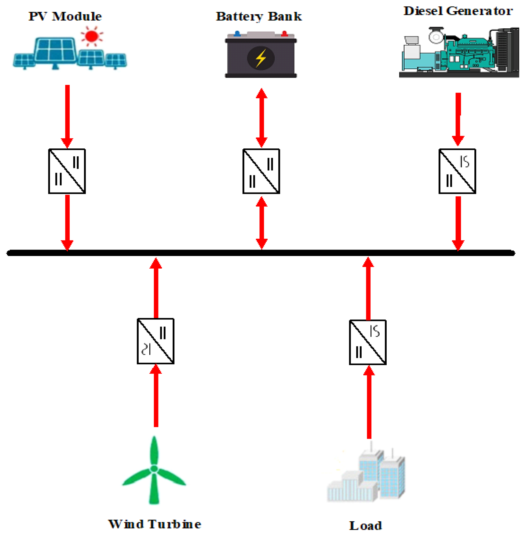
This study was undertaken to design a standalone HRES and run it efficiently. The proposed system combined wind turbines and PV modules as primary energy sources alongside diesel generators and battery banks as backup units. The HRES was intended to supply a residential load. A bi-level optimization problem was established to size the system and optimally manage the energy flow across it. The upper-level sub-problem expressed the sizing task to achieve an optimal economic and environmental performance, i.e., minimizing the total cost and CO₂ emissions. The EMS task was set up in the lower-level sub-problem for achieving the best technoeconomic objectives, i.e., minimizing operating cost and battery degradation. The MATLAB environment was utilized to implement the entire problem, formulated as BMINLP. Specifically, the “intlinprg” solver was used to solve the EMS task, whereas the global optimization solver “ga” was applied to carry out the sizing task.

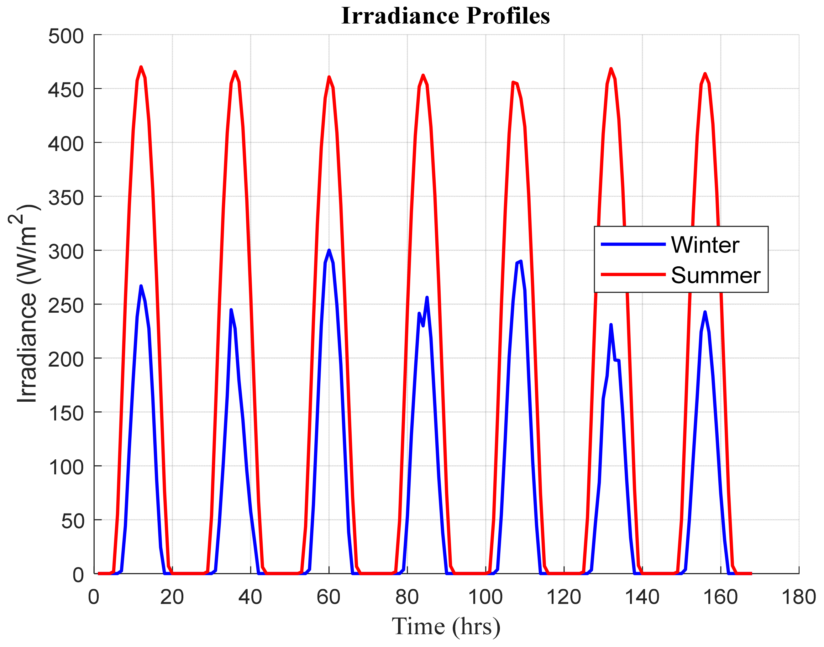
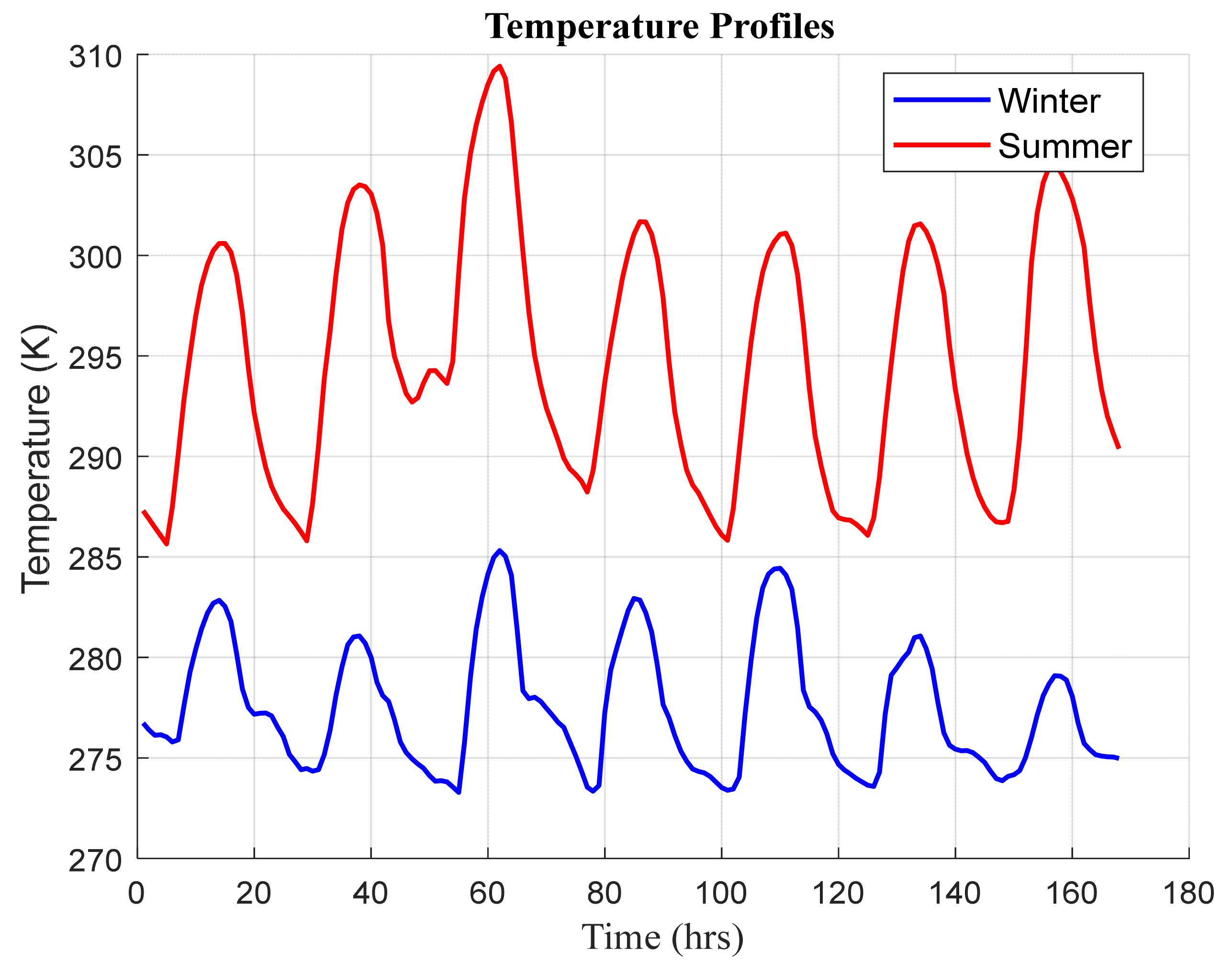
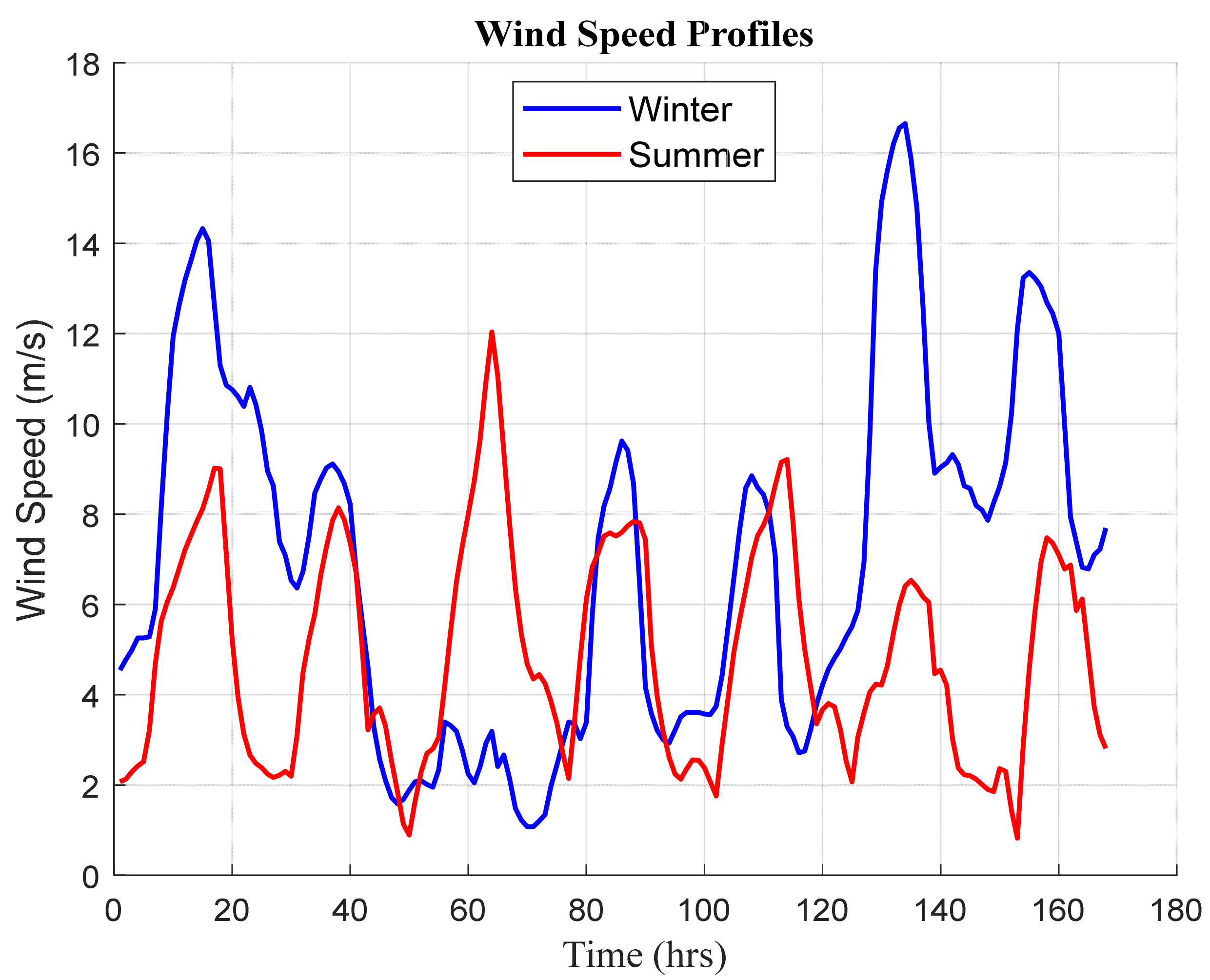
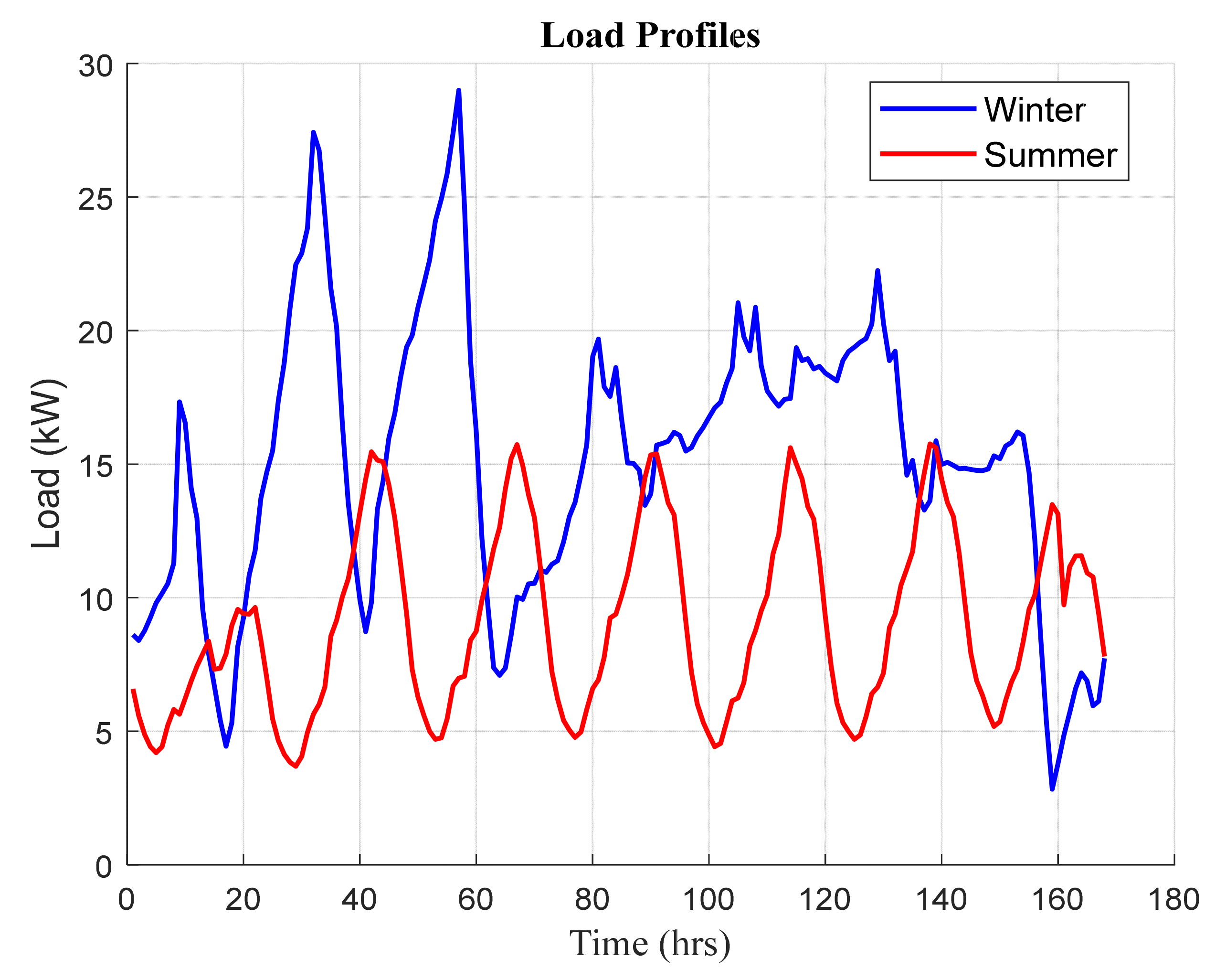
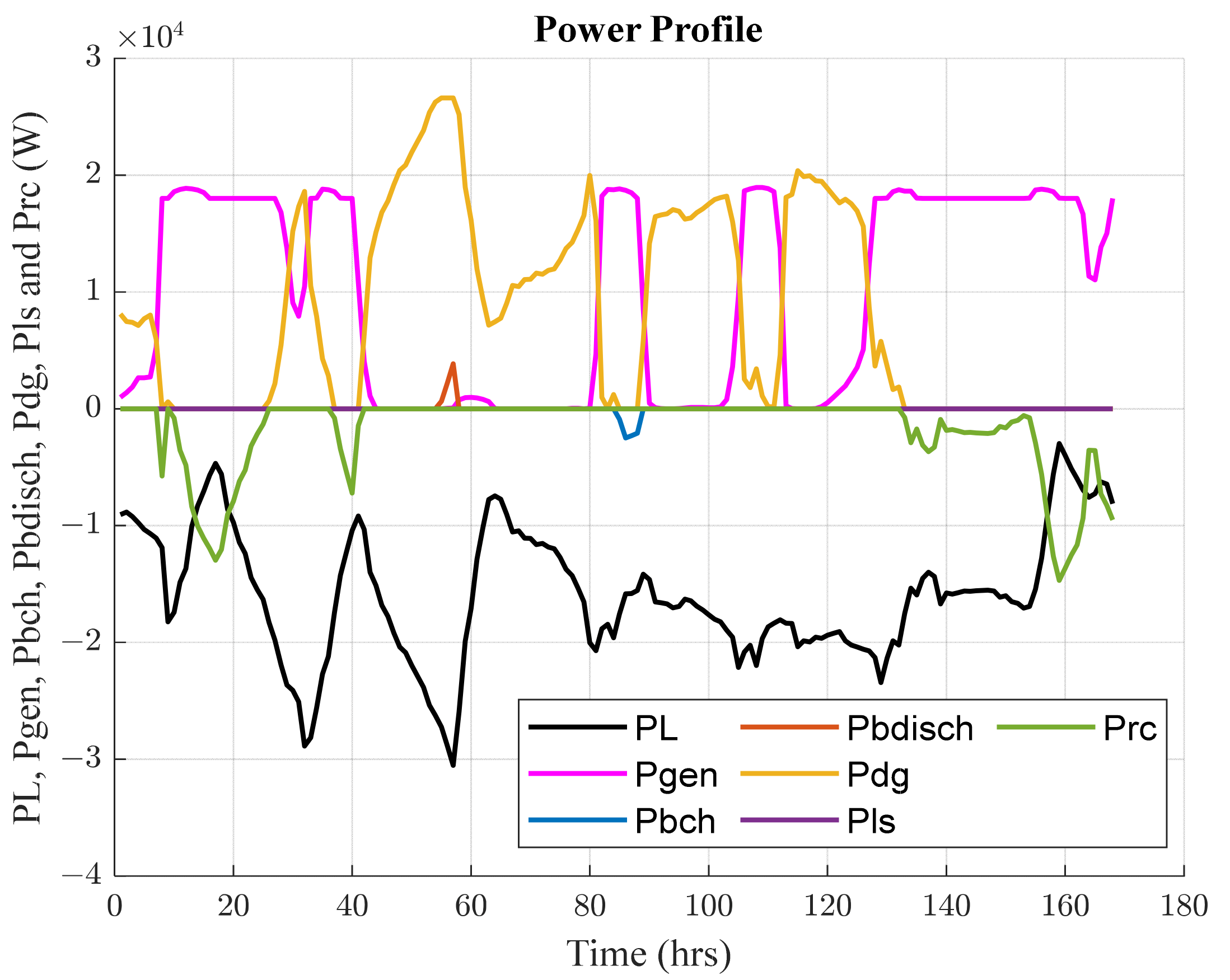
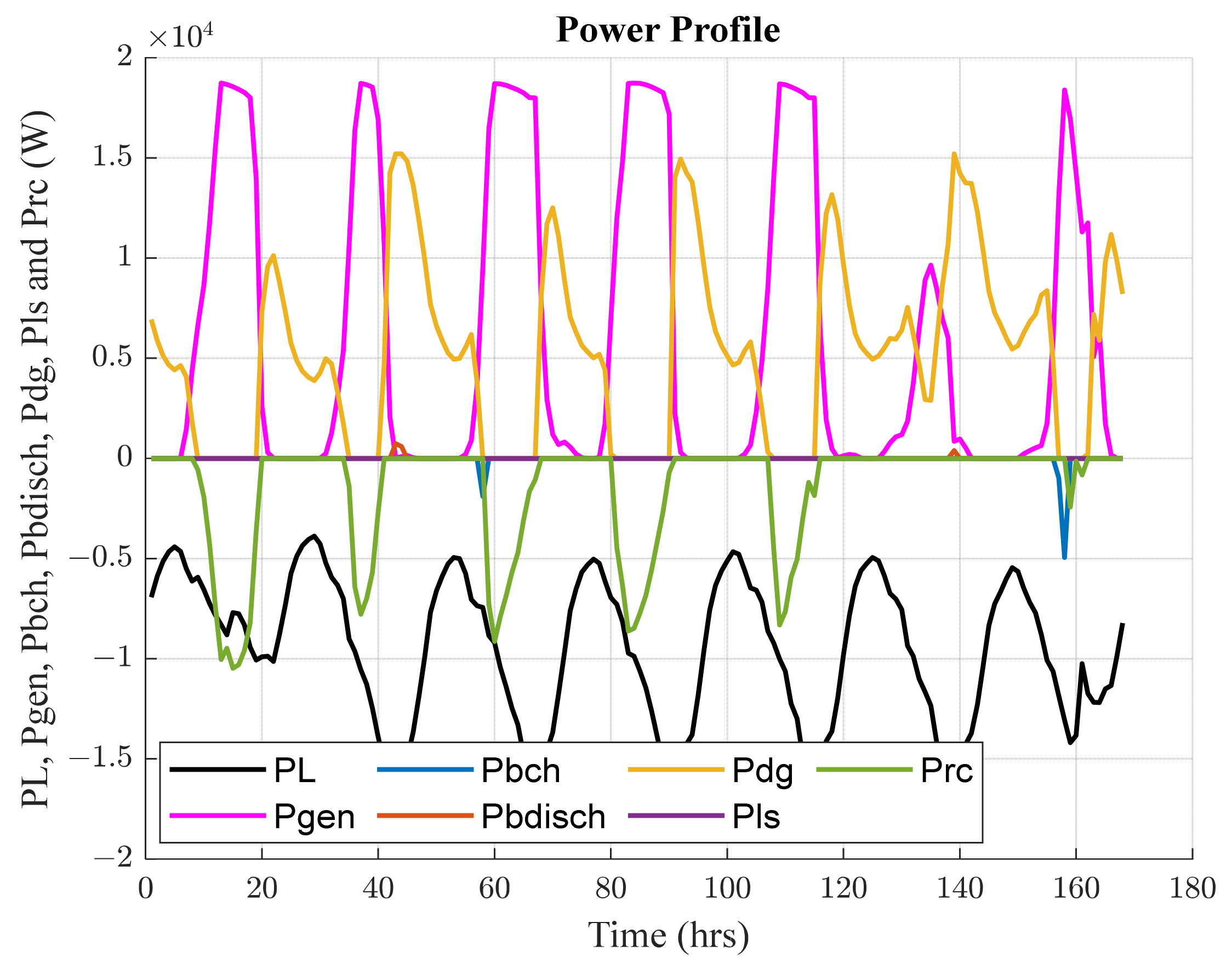
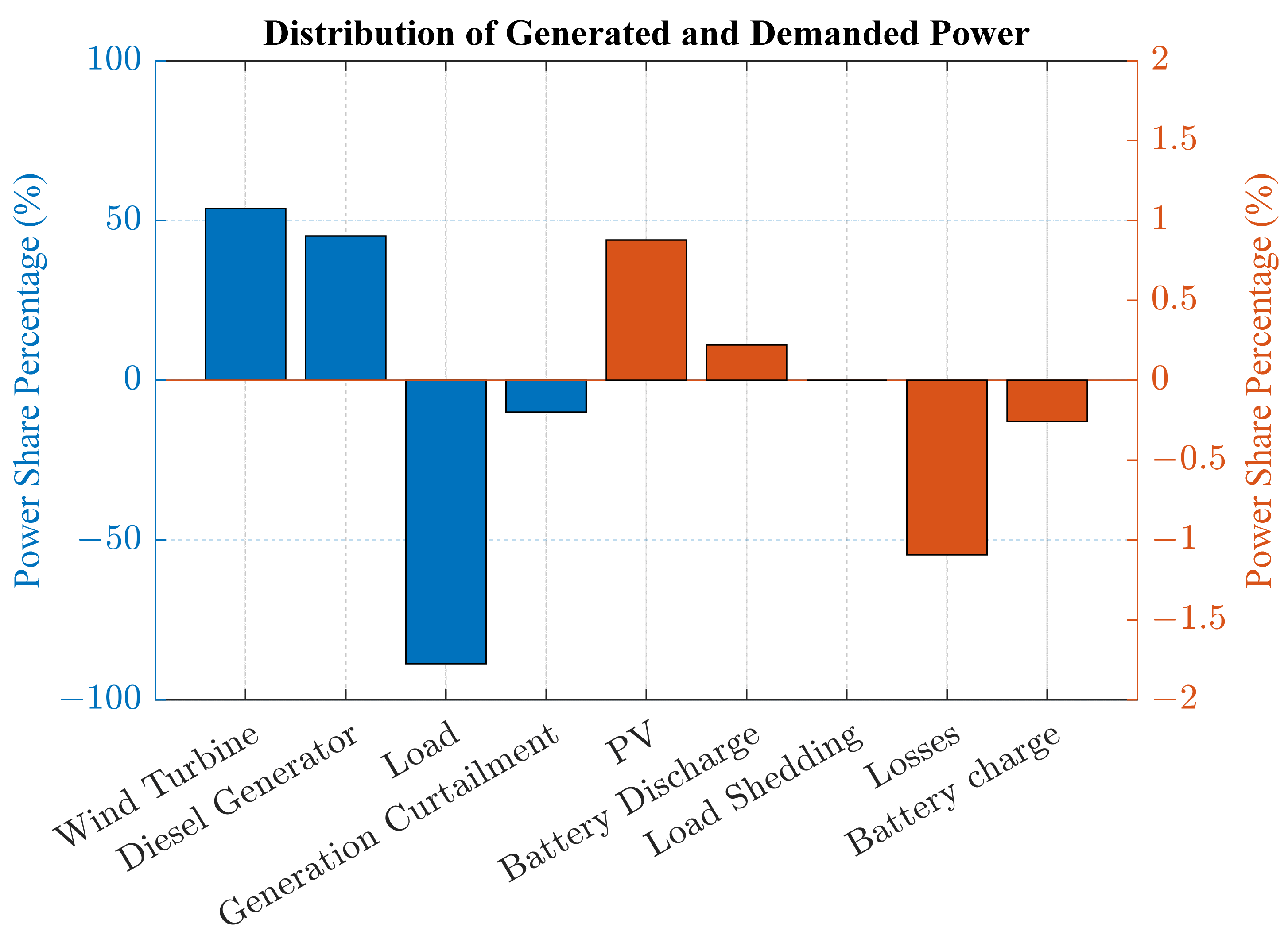
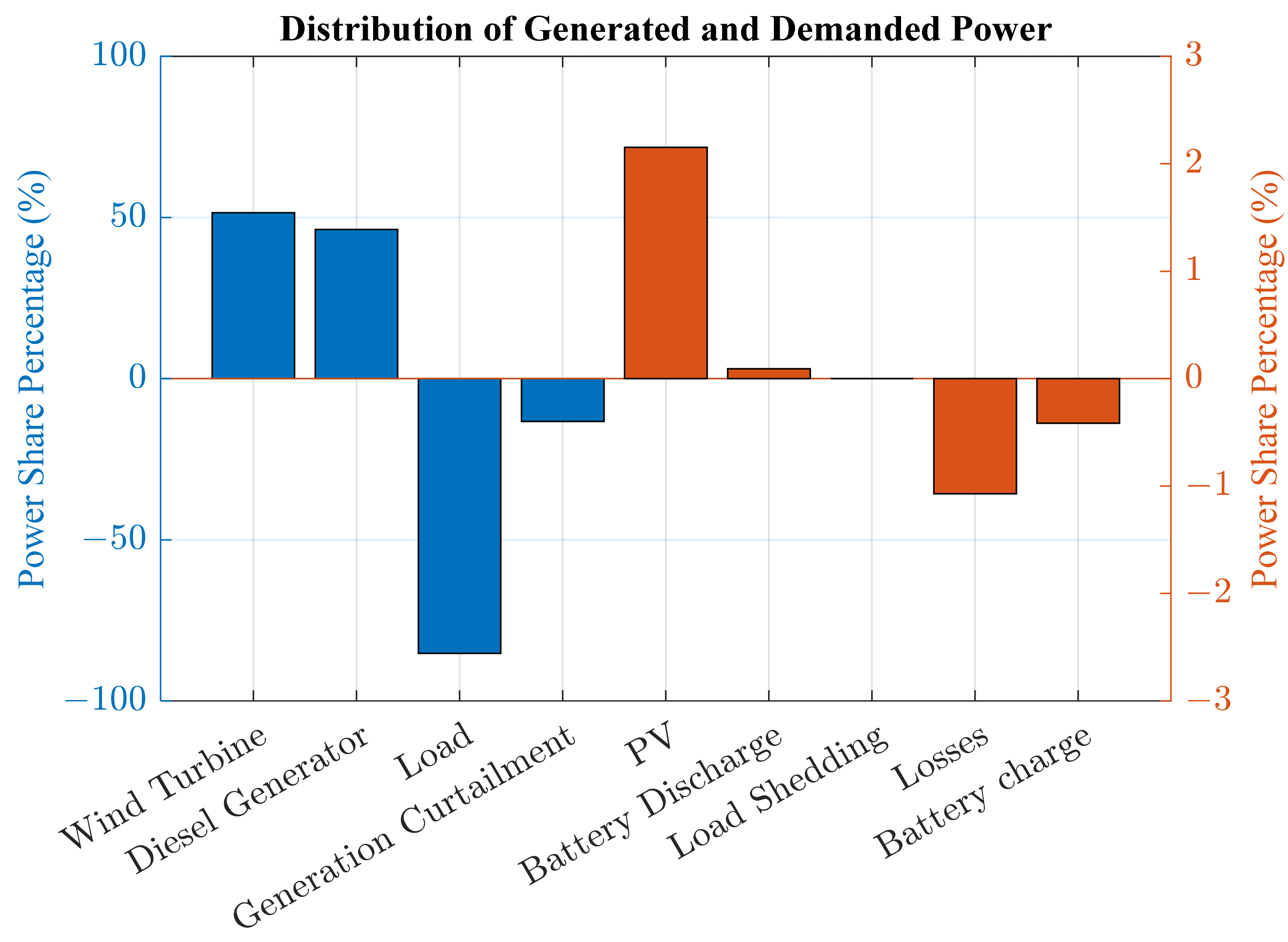
Typical winter and summer weeks were selected as testing periods in the present study. The results were extracted based on the evaluation of certain performance metrics. These metrics included the operating, maintenance, and investment costs, storage unit degradation, and CO₂ emissions. The results indicated that the proposed system attained the best performance during the summer period, compared to the winter period, according to all metrics. In detail, the total cost of the system and the CO₂ emissions recorded USD 26,447.5 and 958.1 kg during the summer week, while the system approximately recorded twice these values, with around USD 43,055.9 and 1585.79 kg during the winter period. Remarkably, the diesel generator was the most contributing component in the operating cost, with at least 96% for both periods. The aforementioned point explains that the system was not invoked to shed loads in case of low renewable generation. One of the most notable findings to emerge from this study was the appearance of two distinguished scenarios. The first one arose when the supplied power was deficient to the load. In such a case, the energy strategy gave priority to the DG to compensate for the shortage of power. Otherwise, the battery was intervened to tackle the issue when the DG reached its limits. On the other hand, the EMS was invoked to reduce the excess generation by a certain value (curtailed power $P_{rc}$), unless the state of charge restriction of the battery allowed it to absorb the surplus generated power.

References

1. Daneshvar, M.; Mohammadi-Ivatloo, B.; Zare, K. An innovative transactive energy architecture for community microgrids in modern multi-carrier energy networks: A Chicago case study. Sci. Rep. 2023, 13, 1529. [Google Scholar] [CrossRef] [PubMed]
2. Belboul, Z.; Toual, B.; Bensalem, A.; Ghenai, C.; Khan, B.; Kamel, S. Techno-economic optimization for isolated hybrid PV/wind/battery/diesel generator microgrid using improved salp swarm algorithm. Sci. Rep. 2024, 14, 2920. [Google Scholar] [CrossRef] [PubMed]
3. Kavadias, K.A.; Triantafyllou, P. Hybrid Renewable Energy Systems’ Optimisation: A Review and Extended Comparison of the Most-Used Software Tools. Energies 2021, 14, 8268. [Google Scholar] [CrossRef]
4. Madhlopa, A.; Sparks, D.; Keen, S.; Moorlach, M.; Krog, P.; Dlamini, T. Optimization of a PV–wind hybrid system under limited water resources. Renew. Sustain. Energy Rev. 2015, 47, 324–331. [Google Scholar] [CrossRef]
5. Walmsley, T.G.; Philipp, M.; Picón-Núñez, M.; Meschede, H.; Taylor, M.T.; Schlosser, F.; Atkins, M.J. Hybrid renewable energy utility systems for industrial sites: A review. Renew. Sustain. Energy Rev. 2023, 188, 113802. [Google Scholar] [CrossRef]
6. Garcia, A.V.M.; Sánchez-Romero, F.J.; López-Jiménez, P.A.; Pérez-Sánchez, M. A new optimization approach for the use of hybrid renewable systems in the search of the zero net energy consumption in water irrigation systems. Renew. Energy 2022, 195, 853–871. [Google Scholar] [CrossRef]
7. Padrón, I.; Avila, D.; Marichal, G.N.; Rodríguez, J.A. Assessment of Hybrid Renewable Energy Systems to supplied energy to Autonomous Desalination Systems in two islands of the Canary Archipelago. Renew. Sustain. Energy Rev. 2018, 101, 221–230. [Google Scholar] [CrossRef]
8. Bahgaat, N.K. Estimation of renewable energy systems for mobile network based on real measurements using HOMER software in Egypt. Sci. Rep. 2023, 13, 16713. [Google Scholar] [CrossRef]
9. Zhang, Z.; Wen, K.; Sun, W. Optimization and sustainability analysis of a hybrid diesel-solar-battery energy storage structure for zero energy buildings at various reliability conditions. Sustain. Energy Technol. Assess. 2023, 55, 102913. [Google Scholar] [CrossRef]
10. Kiptoo, M.K.; Lotfy, M.E.; Adewuyi, O.B.; Conteh, A.; Howlader, A.M.; Senjyu, T. Integrated approach for optimal techno-economic planning for high renewable energy-based isolated microgrid considering cost of energy storage and demand response strategies. Energy Convers. Manag. 2020, 215, 112917. [Google Scholar] [CrossRef]
11. Jiao, P.; Chen, J.; Peng, K.; Zhao, Y.; Xin, K. Multi-objective mean-semi-entropy model for optimal standalone micro-grid planning with uncertain renewable energy resources. Energy 2020, 191, 116497. [Google Scholar] [CrossRef]
12. Muskan; Channi, H.K. Optimal designing of PV-diesel generator-based system using HOMER software. Mater. Today Proc. 2023, 221. [Google Scholar] [CrossRef]
13. Iqbal, R.; Liu, Y.; Zeng, Y.; Zhang, Q.; Zeeshan, M. Comparative study based on techno-economics analysis of different shipboard microgrid systems comprising PV/wind/fuel cell/battery/diesel generator with two battery technologies: A step toward green maritime transportation. Renew. Energy 2024, 221, 119670. [Google Scholar] [CrossRef]
14. Sari, A.; Majdi, A.; Opulencia, M.J.C.; Timoshin, A.; Huy, D.T.N.; Trung, N.D.; Alsaikhan, F.; Hammid, A.T.; Akhmedov, A. New optimized configuration for a hybrid PV/diesel/battery system based on coyote optimization algorithm: A case study for Hotan county. Energy Rep. 2022, 8, 15480–15492. [Google Scholar] [CrossRef]
15. Maheri, A.; Unsal, I.; Mahian, O. Multiobjective optimisation of hybrid wind-PV-battery-fuel cell-electrolyser-diesel systems: An integrated configuration-size formulation approach. Energy 2021, 241, 122825. [Google Scholar] [CrossRef]
16. Bacha, B.; Ghodbane, H.; Dahmani, H.; Betka, A.; Toumi, A.; Chouder, A. Optimal sizing of a hybrid microgrid system using solar, wind, diesel, and battery energy storage to alleviate energy poverty in a rural area of Biskra, Algeria. J. Energy Storage 2024, 84, 110651. [Google Scholar] [CrossRef]
17. Al-Quraan, A.; Al-Mhairat, B. Sizing and energy management of standalone hybrid renewable energy systems based on economic predictive control. Energy Convers. Manag. 2024, 300, 117948. [Google Scholar] [CrossRef]
18. Liu, W.H.; Alwi, S.R.W.; Hashim, H.; Lim, J.S.; Rozali, N.E.M.; Ho, W.S. Sizing of Hybrid Power System with varying current type using numerical probabilistic approach. Appl. Energy 2016, 184, 1364–1373. [Google Scholar] [CrossRef]
19. Nogueira, C.E.C.; Vidotto, M.L.; Niedzialkoski, R.K.; de Souza, S.N.M.; Chaves, L.I.; Edwiges, T.; dos Santos, D.B.; Werncke, I. Sizing and simulation of a photovoltaic-wind energy system using batteries, applied for a small rural property located in the south of Brazil. Renew. Sustain. Energy Rev. 2014, 29, 151–157. [Google Scholar] [CrossRef]
20. Mahesh, A.; Sandhu, K.S. Hybrid Wind/Photovoltaic Energy System Developments: Critical Review and Findings. Renew. Sustain. Energy Rev. 2015, 52, 1135–1147. [Google Scholar] [CrossRef]
21. Ammari, C.; Belatrache, D.; Touhami, B.; Makhloufi, S. Sizing, optimization, control and energy management of hybrid renewable energy system—A review. Energy Built Environ. 2022, 3, 399–411. [Google Scholar] [CrossRef]
22. Rekioua, D.; Mokrani, Z.; Kakouche, K.; Rekioua, T.; Oubelaid, A.; Logerais, P.O.; Ali, E.; Bajaj, M.; Berhanu, M.; Ghoneim, S.S.M. Optimization and intelligent power management control for an autonomous hybrid wind turbine photovoltaic diesel generator with batteries. Sci. Rep. 2023, 13, 21830. [Google Scholar] [CrossRef] [PubMed]
23. Al-Quraan, A.; Athamnah, I. Economic tri-level control-based sizing and energy management optimization for efficiency maximization of stand-alone HRES. Energy Convers. Manag. 2024, 302, 118140. [Google Scholar] [CrossRef]
24. Al-Quraan, A.; Athamnah, I. Economic predictive tri-level control for efficiency maximization of stand-alone hybrid renewable energy system. J. Power Sources 2024, 596, 234098. [Google Scholar] [CrossRef]
25. Nair, S.P.; Sundari, S. Optimizing day-ahead energy management with demand response in a PV-diesel-battery system using a hybrid GOA-SNN strategy. J. Energy Storage 2024, 76, 109717. [Google Scholar] [CrossRef]
26. Alarcón, M.A.; Alarcón, R.G.; González, A.H.; Ferramosca, A. Economic model predictive control for energy management of a microgrid connected to the main electrical grid. J. Process. Control. 2022, 117, 40–51. [Google Scholar] [CrossRef]
27. Zou, B.; Peng, J.; Yin, R.; Luo, Z.; Song, J.; Ma, T.; Li, S.; Yang, H. Energy management of the grid-connected residential photovoltaic-battery system using model predictive control coupled with dynamic programming. Energy Build. 2023, 279, 112712. [Google Scholar] [CrossRef]
28. Manzano, J.; Salvador, J.; Romaine, J.; Alvarado-Barrios, L. Economic predictive control for isolated microgrids based on real world demand/renewable energy data and forecast errors. Renew. Energy 2022, 194, 647–658. [Google Scholar] [CrossRef]
29. Vand, B.; Ruusu, R.; Hasan, A.; Delgado, B.M. Optimal management of energy sharing in a community of buildings using a model predictive control. Energy Convers. Manag. 2021, 239, 114178. [Google Scholar] [CrossRef]
30. Liang, B.; Liu, W.; Sun, L.; He, Z.; Hou, B. Economic MPC-Based smart home scheduling with comprehensive load types, real-time tariffs, and intermittent DERs. IEEE Access 2020, 8, 194373–194383. [Google Scholar] [CrossRef]
31. Yu, Y.; Li, J.; Chen, D. Optimal dispatching method for integrated energy system based on robust economic model predictive control considering source–load power interval prediction. Glob. Energy Interconnect. 2022, 5, 564–578. [Google Scholar] [CrossRef]
32. Luo, X.; Liu, Y.; Liu, X. Bi-level multi-objective optimization of design and subsidies for standalone hybrid renewable energy systems: A novel approach based on artificial neural network. J. Build. Eng. 2021, 41, 102744. [Google Scholar] [CrossRef]
33. Wang, D.; Liu, Y.; Wang, Y.; Shi, X.; Song, X. Allocation of coal de-capacity quota among provinces in China: A bi-level multi-objective combinatorial optimization approach. Energy Econ. 2020, 87, 104709. [Google Scholar] [CrossRef]
34. Wu, C.; Gu, W.; Xu, Y.; Jiang, P.; Lu, S.; Zhao, B. Bi-level optimization model for integrated energy system considering the thermal comfort of heat customers. Appl. Energy 2018, 232, 607–616. [Google Scholar] [CrossRef]
35. The MathWorks Inc. Optimization Toolbox, Version 9.4 (R2022b); The MathWorks Inc.: Natick, MA, USA, 2022.
36. Solarypsi. August 2011. Available online: https://www.solarypsi.org/repository/documents/adamsschool/SunModule_Poly_240_Data_Sheet.pdf (accessed on 5 February 2024).
37. Masters, G.M. Renewable and Efficient Electric Power Systems; John Wiley & Sons, Inc.: Hoboken, NJ, USA, 2004. [Google Scholar]
38. Katsivelakis, M.; Bargiotas, D.; Daskalopulu, A.; Panapakidis, I.P.; Tsoukalas, L. Techno-Economic Analysis of a Stand-Alone Hybrid System: Application in Donoussa Island, Greece. Energies 2021, 14, 1868. [Google Scholar] [CrossRef]
39. Shi, Z.; Wang, R.; Zhang, T. Multi-objective optimal design of hybrid renewable energy systems using preference-inspired coevolutionary approach. Sol. Energy 2015, 118, 96–106. [Google Scholar] [CrossRef]
40. Technical Specification for Vented Lead-Acid Batteries (VLA). Available online: https://www.baebatteriesusa.com/wp-content/uploads/2018/12/BAE_PVS_Cell_en_2016.06-B.pdf (accessed on 5 February 2024).
41. Abbassi, M.; Chaabani, A.; Ben Said, L.; Absi, N. Bi-level multi-objective combinatorial optimization using reference approximation of the lower level reaction. Procedia Comput. Sci. 2020, 176, 2098–2107. [Google Scholar] [CrossRef]
42. Bui, L.T.; Alam, S. Multi-Objective Optimization in Computational Intelligence: Theory and Practice; IGI Global: Hershey, PA, USA, 2008. [Google Scholar]
43. García-Triviño, P.; Fernández-Ramírez, L.M.; Gil-Mena, A.J.; Llorens-Iborra, F.; García-Vázquez, C.A.; Jurado, F. Optimized operation combining costs, efficiency and lifetime of a hybrid renewable energy system with energy storage by battery and hydrogen in grid-connected applications. Int. J. Hydrogen Energy 2016, 41, 23132–23144. [Google Scholar] [CrossRef]
44. Zhao, J.; Yuan, X. Multi-objective optimization of stand-alone hybrid PV-wind-diesel-battery system using improved fruit fly optimization algorithm. Soft Comput. 2015, 20, 2841–2853. [Google Scholar] [CrossRef]
45. Garcia, R.S.; Weisser, D. A wind–diesel system with hydrogen storage: Joint optimisation of design and dispatch. Renew. Energy 2006, 31, 2296–2320. [Google Scholar] [CrossRef]
46. NASA. Prediction of Worldwide Energy Resources (POWER). Available online: https://power.larc.nasa.gov/ (accessed on 5 February 2024).
47. OpenEI. Open Energy Information Datasets. Available online: https://openei.org/datasets/files/961/pub/ (accessed on 5 February 2024).
48. Mayernik, J.; Office of Energy Efficiency & Renewable Energy (EERE). Buildings Energy Data Book; National Renewable Energy Laboratory: Golden, CO, USA, 2015. Available online: https://data.openei.org/submissions/144 (accessed on 5 February 2024).
49. Google Earth. Geographical Location of Udhruh, Southern Jordan. Available online: https://earth.google.com/web/search/%d8%a3%d8%b0%d8%b1%d8%ad/@30.33680815,35.59963306,1307.88644268a,8214.25246558d,35y,0h,0t,0r (accessed on 5 February 2024).
Figure 1. The basic illustration of the proposed BMINLP technique.
Sustainability 17 00725 g001
Figure 2. The graphic illustration of the suggested HRES.
Sustainability 17 00725 g002
Figure 3. The detailed steps of the methodology.
Sustainability 17 00725 g003
Figure 4. Irradiance profiles of the designated weeks.
Sustainability 17 00725 g004
Figure 5. Temperature profiles of the designated weeks.
Sustainability 17 00725 g005
Figure 6. Wind speed profiles of the designated weeks.
Sustainability 17 00725 g006
Figure 7. Load profiles of the designated weeks.
Sustainability 17 00725 g007
Figure 8. Topographical location of the selected site [49].
Sustainability 17 00725 g008
Figure 9. Power profiles of the winter week.
Sustainability 17 00725 g009
Figure 10. Power profiles of the summer week.
Sustainability 17 00725 g010
Figure 11. The share of power distribution for the winter week.
Sustainability 17 00725 g011
Figure 12. The share of power distribution for the summer week.
Sustainability 17 00725 g012