

Effectiveness of a Series of Road Humps on Home Zone Streets: A Case Study


Abstract
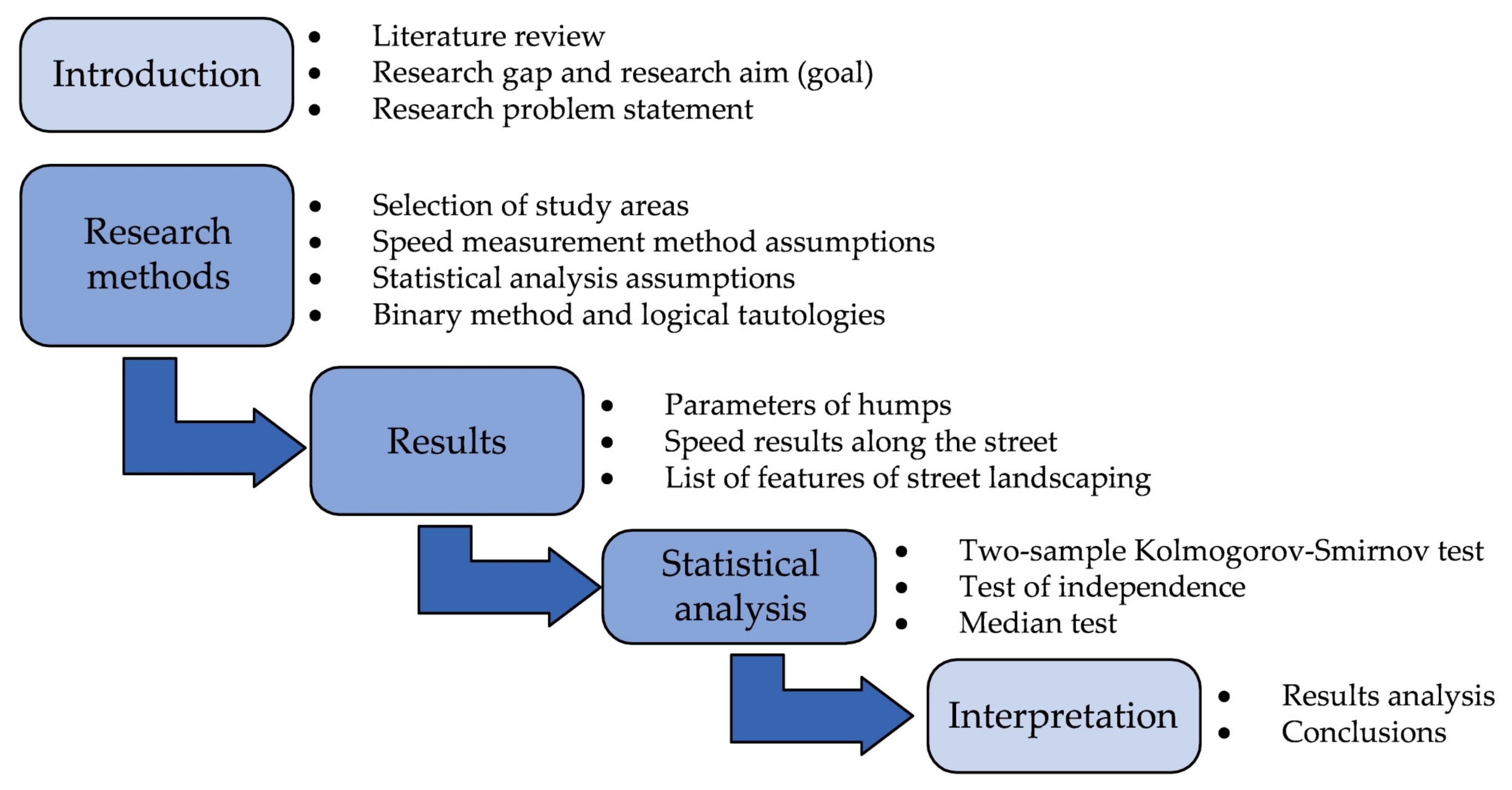
1. Introduction
- ①
- “Which hump type (ST or SH) is more effective in slowing down traffic in home zones?”
- ②
- “Is the direction of travel on a two-way roadway relevant to the speed on home zone streets with different longitudinal gradients?”
- ③
- “Are there any other factors related to street landscaping in home zones that may contribute to maintaining a slowing effect along the street?”
2. Research Assumptions and the Applied Methods
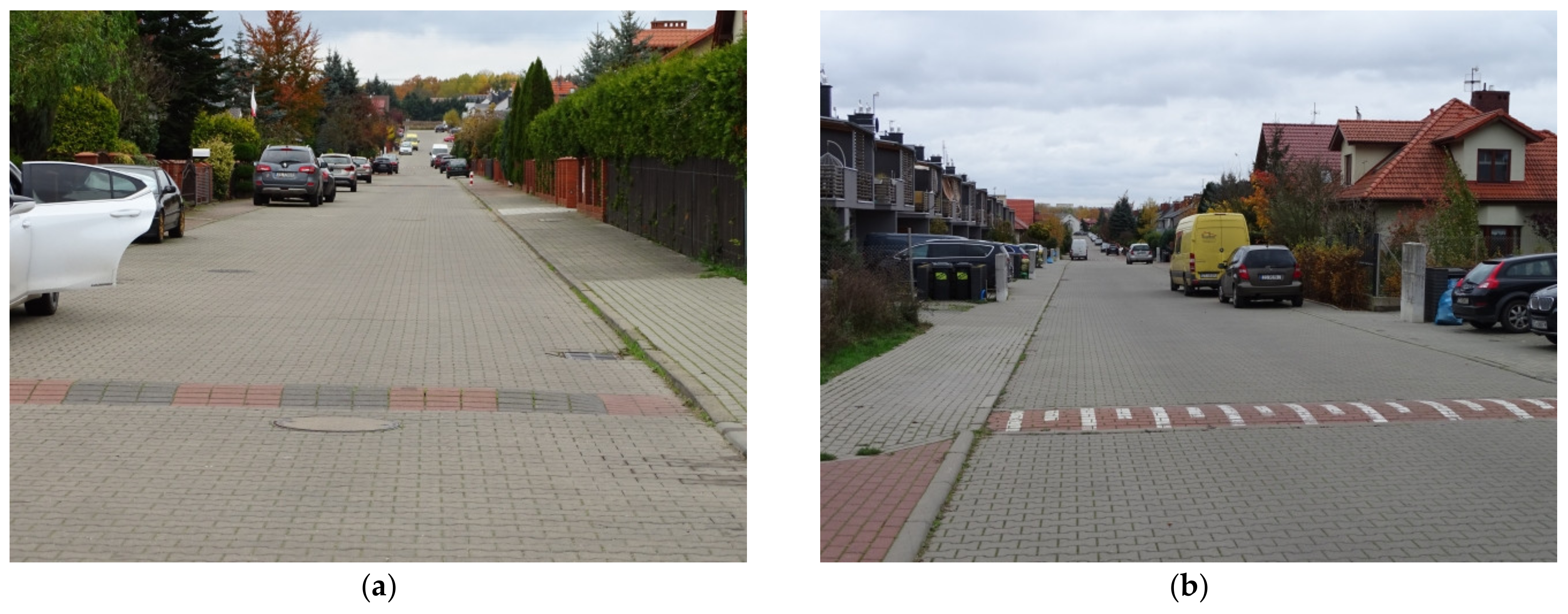
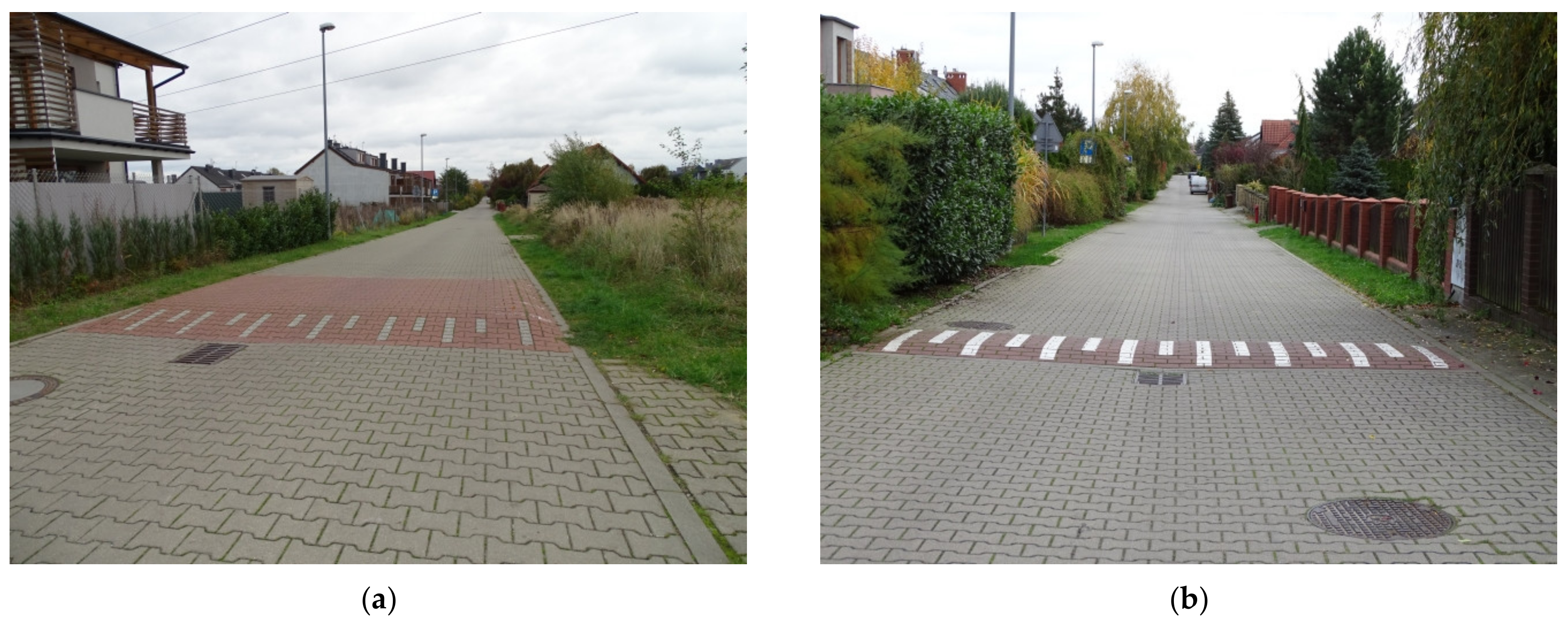
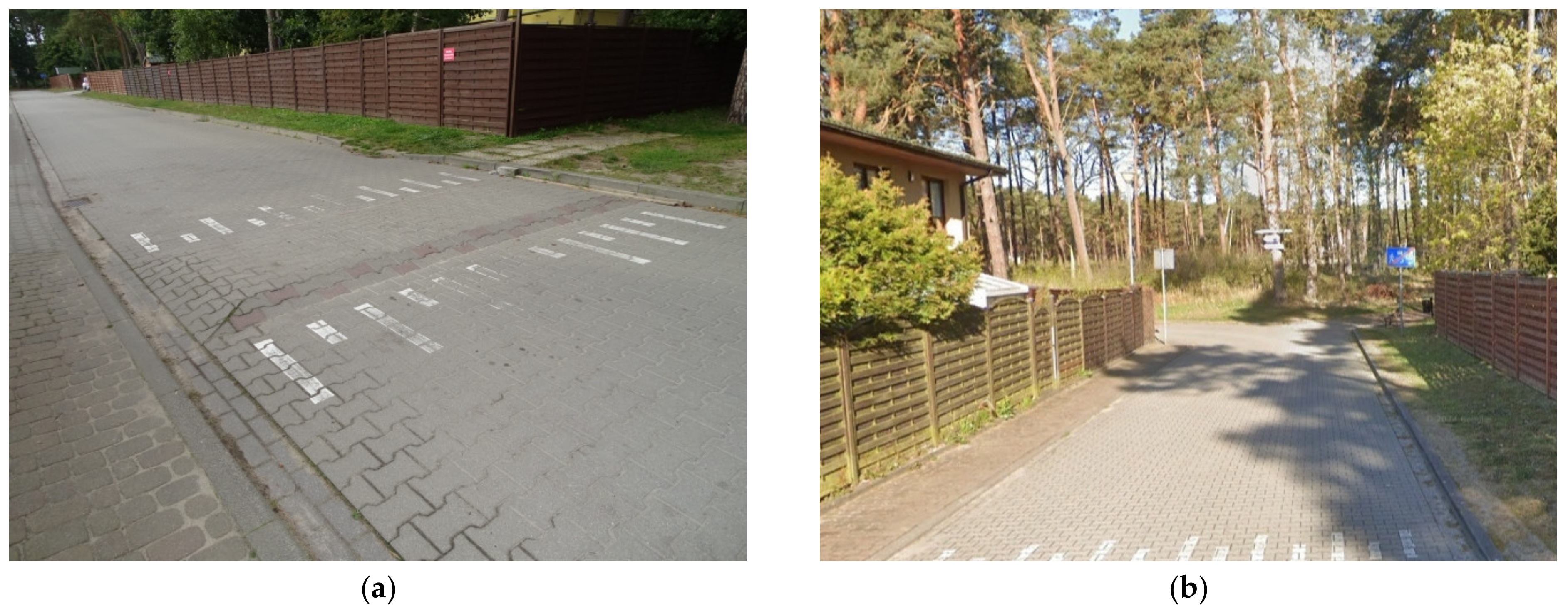
2.1. Study Areas Research Assumptions Applied in Study Area Selection
- –
- The street should be located in a home zone occupied by single-family buildings.
- –
- There should be home zone traffic signs placed at the beginning and end of the street.
- –
- Only two-way streets having roadways of similar widths will be considered.
- –
- The horizontal alignment should follow a straight line, and the vertical alignment should vary.
- –
- The street should include a few humps of different types placed at different spacing intervals, and their spacing should be very diverse.
- –
- There may or may not be a sidewalk running along the street, and it may be separated from properties using fences or hedgerows.
- –
- There must be parking facilities provided on the street on one or two sides, with the parking spaces situated parallel or at a right angle to the roadway axis.
- –
- Only passenger cars and municipal vehicles should be allowed to travel along the street.
2.2. Speed Survey Research Assumptions and Measurement Methods
2.3. Statistical Analysis Assumptions and Selection of Appropriate Statistical Tests
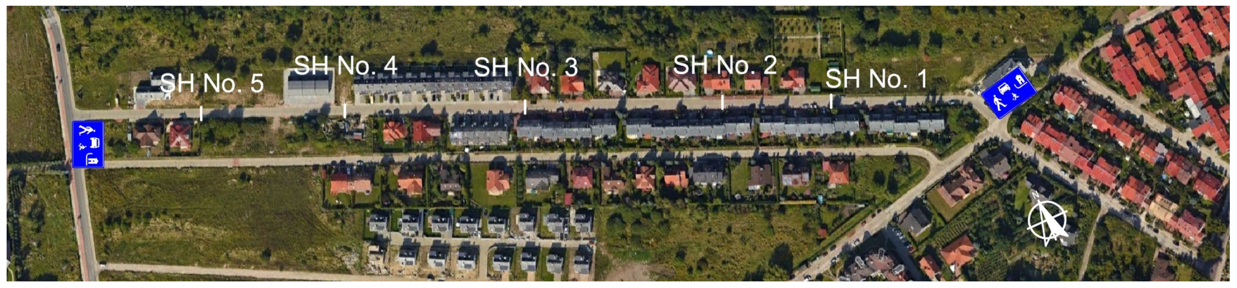
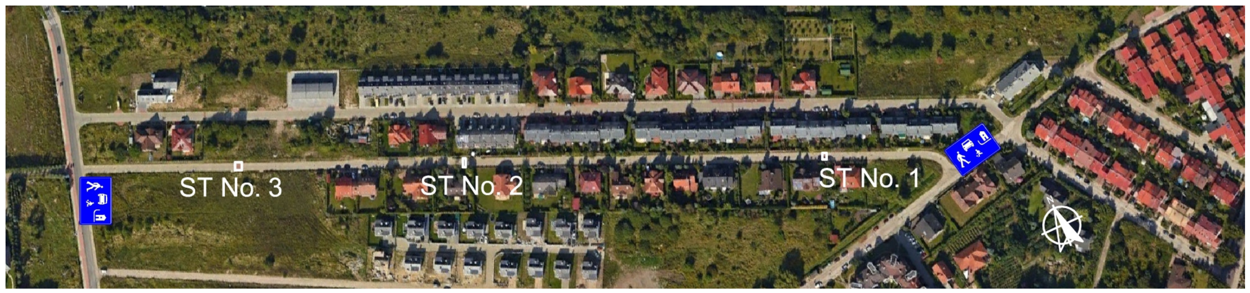
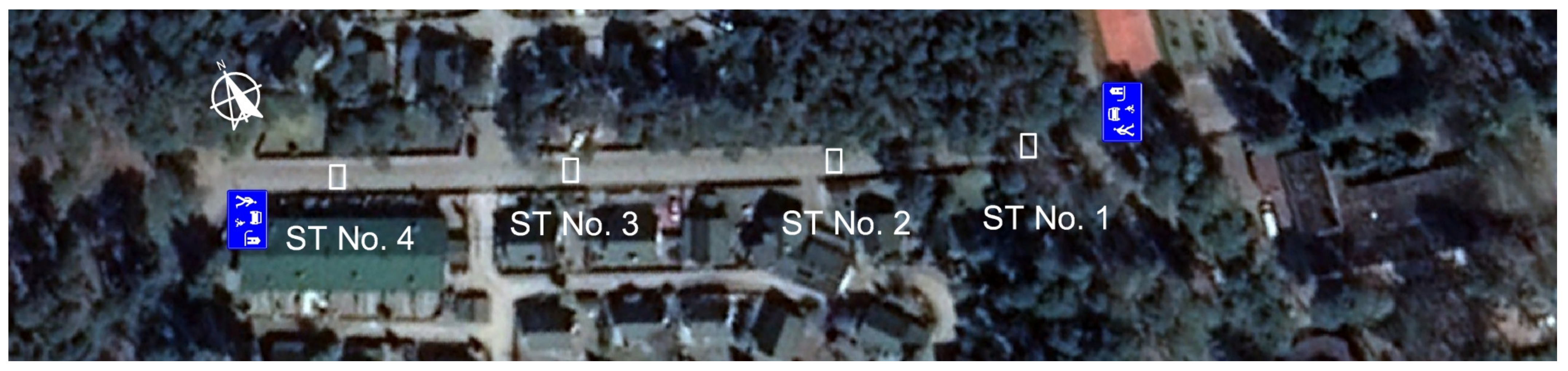
3. Chosen Study Areas

| Hump No. | Geometric Parameters | |||||||||||||
|---|---|---|---|---|---|---|---|---|---|---|---|---|---|---|
| ibefore | i1 | h1 | l1 | lg | lt | l2 | h2 | i2 | iafter | lentry | lexit | z | l3 | |
| Study area A | ||||||||||||||
| 1 | 0.40 | 21.0 | 8.4 | 0.40 | 0.20 | 1.00 | 0.40 | 6.1 | −15.25 | 0.40 | 70 | – | 96 | 0.2 |
| 2 | 0.25 | 21.0 | 8.0 | 0.40 | 0.20 | 1.00 | 0.40 | 7.0 | −17.5 | 0.25 | – | – | 135 | 0.2 |
| 3 | 1.10 | 12.2 | 6.1 | 0.50 | 0.20 | 1.44 | 0.50 | 5.2 | −10.4 | 2.10 | – | – | 129 | 0.2 |
| 4 | 3.50 | 17.0 | 6.8 | 0.40 | 0.20 | 1.44 | 0.60 | 5.0 | −8.3 | 3.10 | – | – | 93 | 0.2 |
| 5 | 4.75 | 23.9 | 9.8 | 0.41 | 0.16 | 0.93 | 0.36 | 6.4 | −17.8 | 2.60 | – | 93 | – | 0.2 |
| Study area B | ||||||||||||||
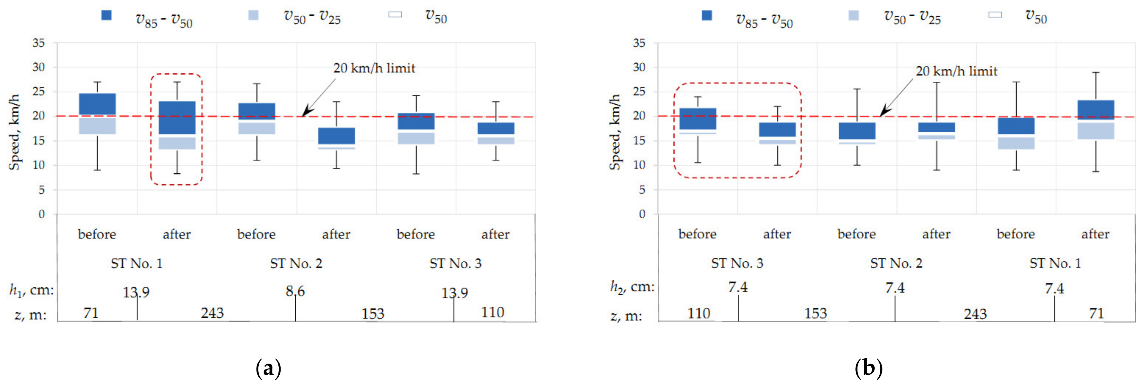
| 1 | 0.90 | 16.3 | 13.9 | 0.85 | 2.49 | 4.28 | 0.95 | 7.4 | −7.8 | 0.90 | 71 | – | 243 | 0.0 |
| 2 | 2.50 | 21.5 | 8.6 | 0.40 | 0.70 | 1.50 | 0.40 | 7.4 | −18.5 | 1.35 | – | – | 153 | 0.0 |
| 3 | 3.70 | 14.3 | 13.9 | 0.97 | 2.47 | 4.59 | 1.15 | 7.4 | −6.4 | 3.20 | – | 109 | – | 0.2 |
| Study area C | ||||||||||||||
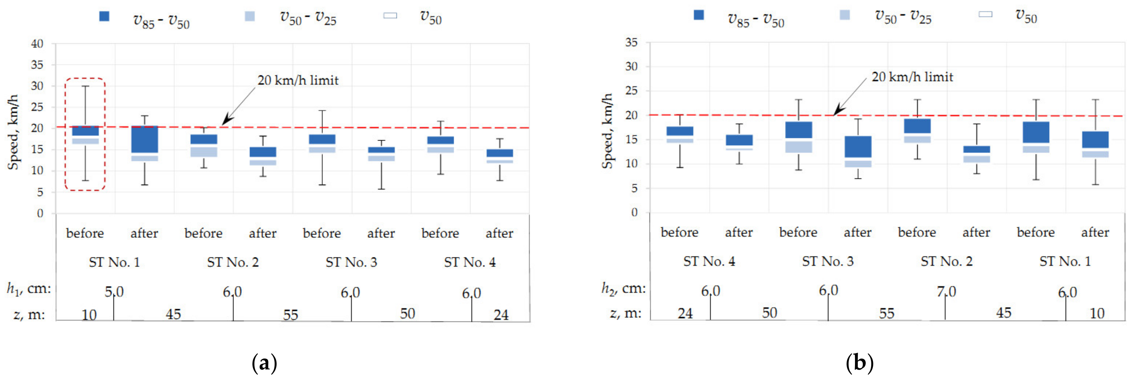
| 1 | 0.10 | 19.2 | 5.0 | 0.26 | 1.00 | 1.95 | 0.69 | 6.0 | −8.7 | 0.10 | 10 | – | 45 | 0.2 |
| 2 | −0.40 | 13.3 | 6.0 | 0.45 | 0.80 | 1.70 | 0.45 | 7.0 | −15.5 | −0.40 | – | – | 55 | 0.2 |
| 3 | −0.40 | 17.1 | 6.0 | 0.35 | 1.00 | 1.70 | 0.35 | 6.0 | −17.1 | −0.40 | – | – | 50 | 0.2 |
| 4 | −0.30 | 17.1 | 6.0 | 0.35 | 1.00 | 1.70 | 0.35 | 6.0 | −17.1 | −0.30 | – | 24 | – | 0.2 |
4. Result
4.1. Results Obtained in the Study Area A
4.2. Result Obtained in Study Area B
4.3. Result Obtained in Study Area C
4.4. Results of Other Statistical Tests
- –
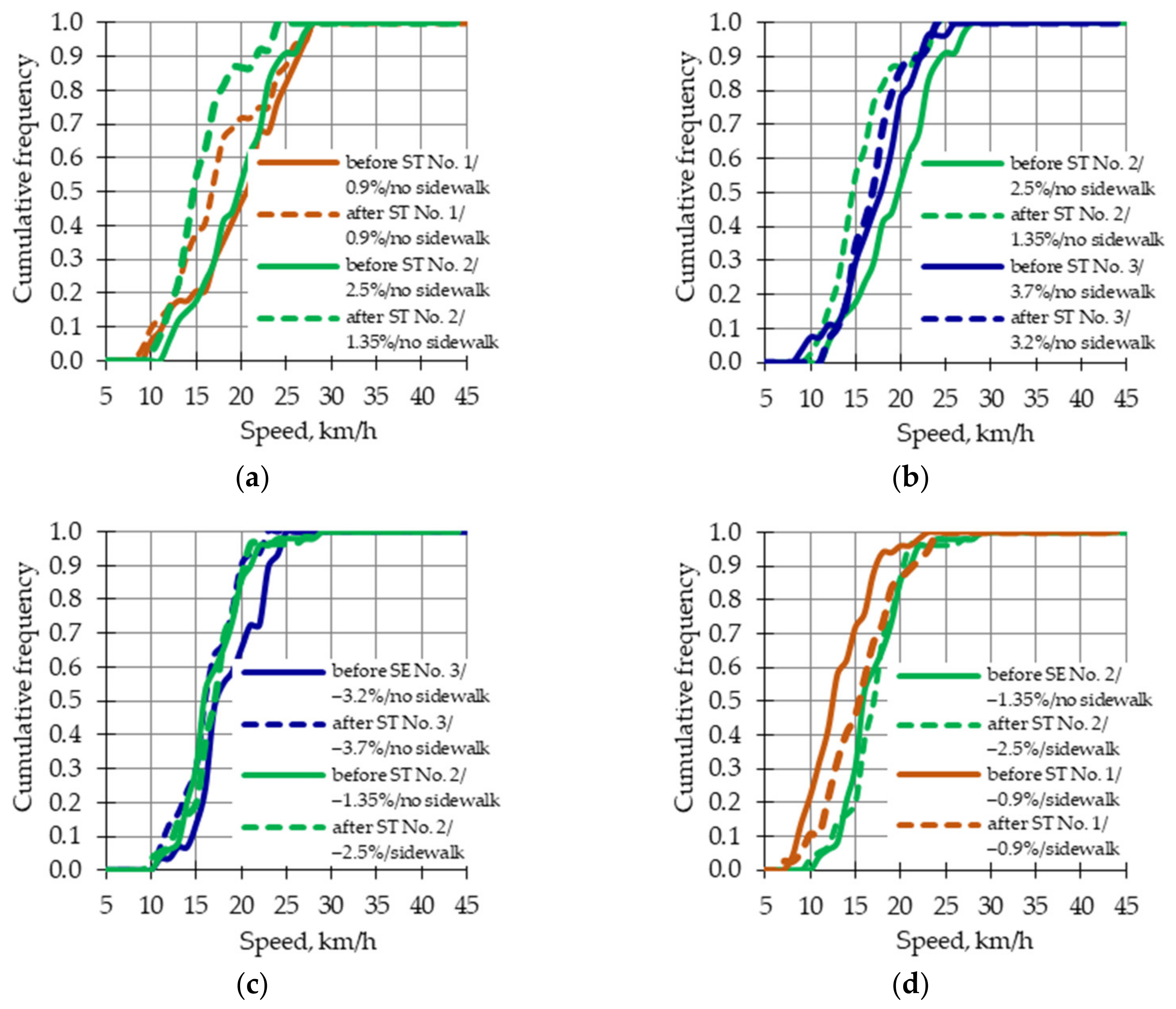
- Street longitudinal gradient (study area A—speed hump No. 1 ≈ 0.4% and speed hump No. 5: 4.75% and 2.6%; study area B—speed table No. 1 at 0.9% and speed table No. 3—3.7% and 3.2%; study area C—speed table No. 1 at 0.1% and speed table No. 4 at −0.3%);
- –
- Distance from the entry point to the first hump or distance from the last hump to the end of the street (study area A—speed hump No. 1 at 70 m and speed hump No. 5—93 m; study area B—speed table No. 1 at 71 m and speed table No. 3—109 m; study area C—speed table No. 1 at 10 m and speed table No. 4—24 m);
- –
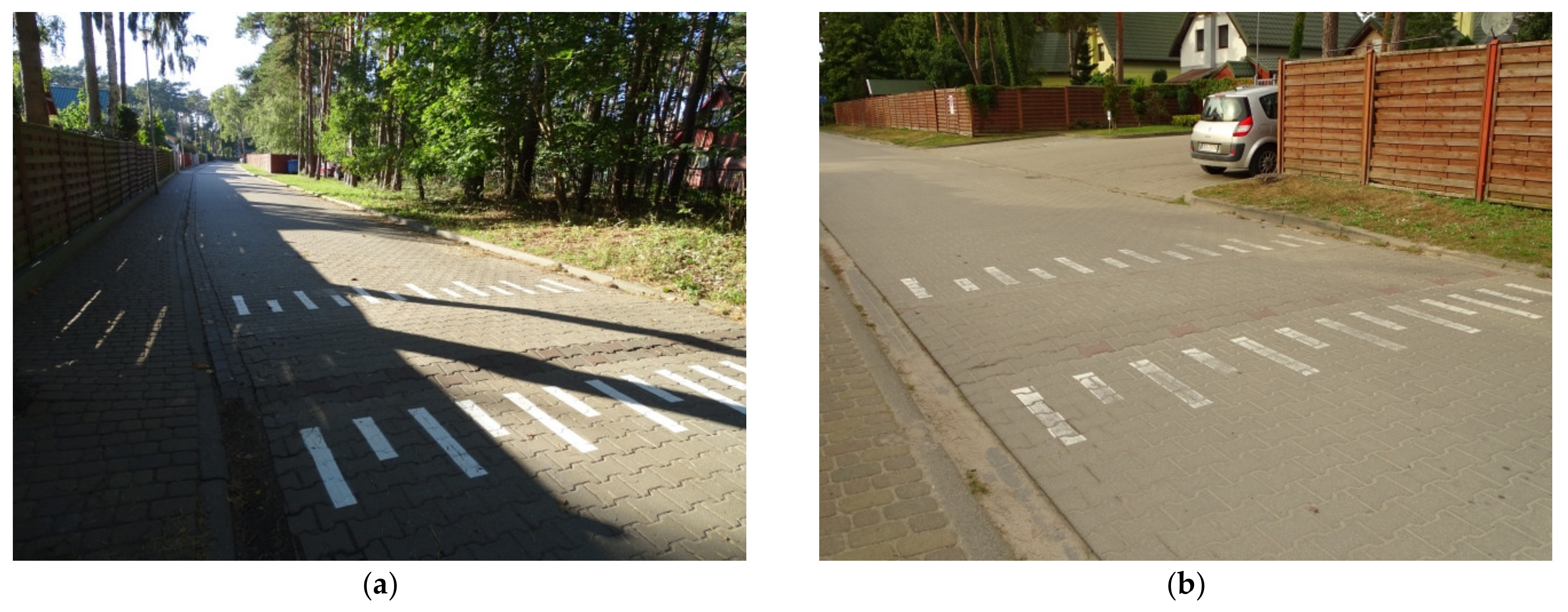
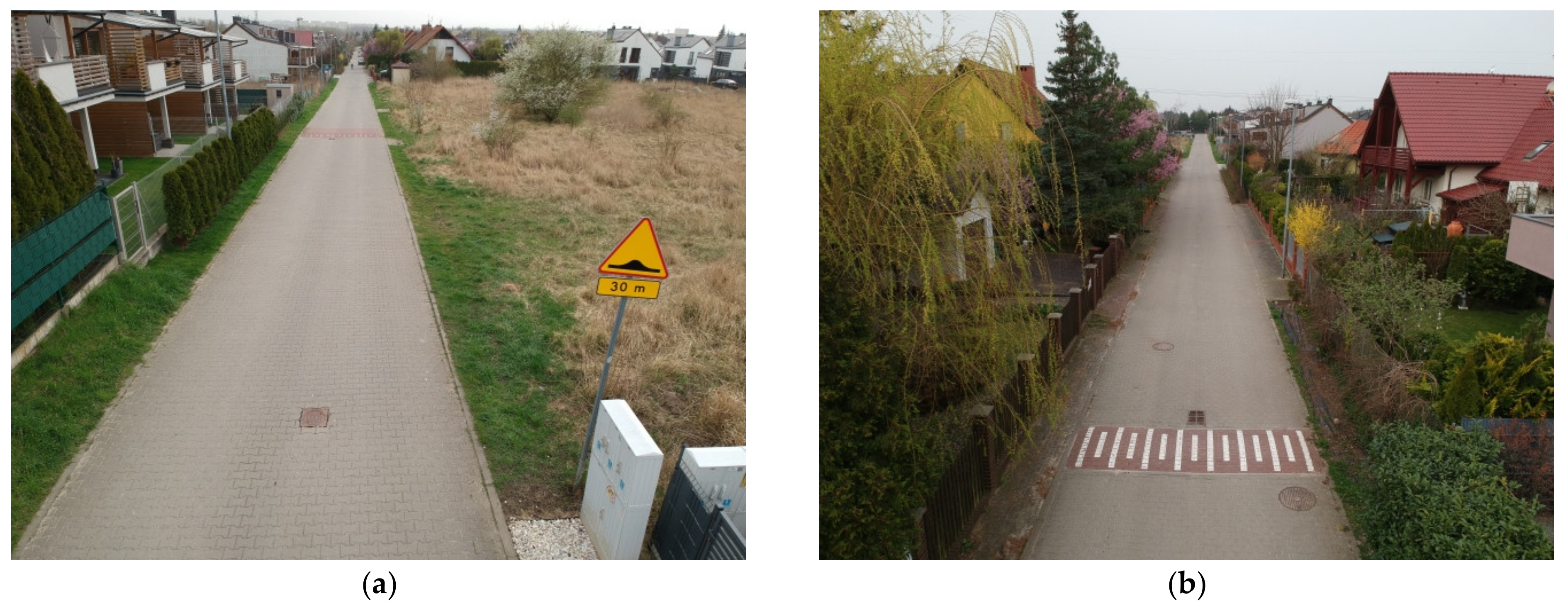
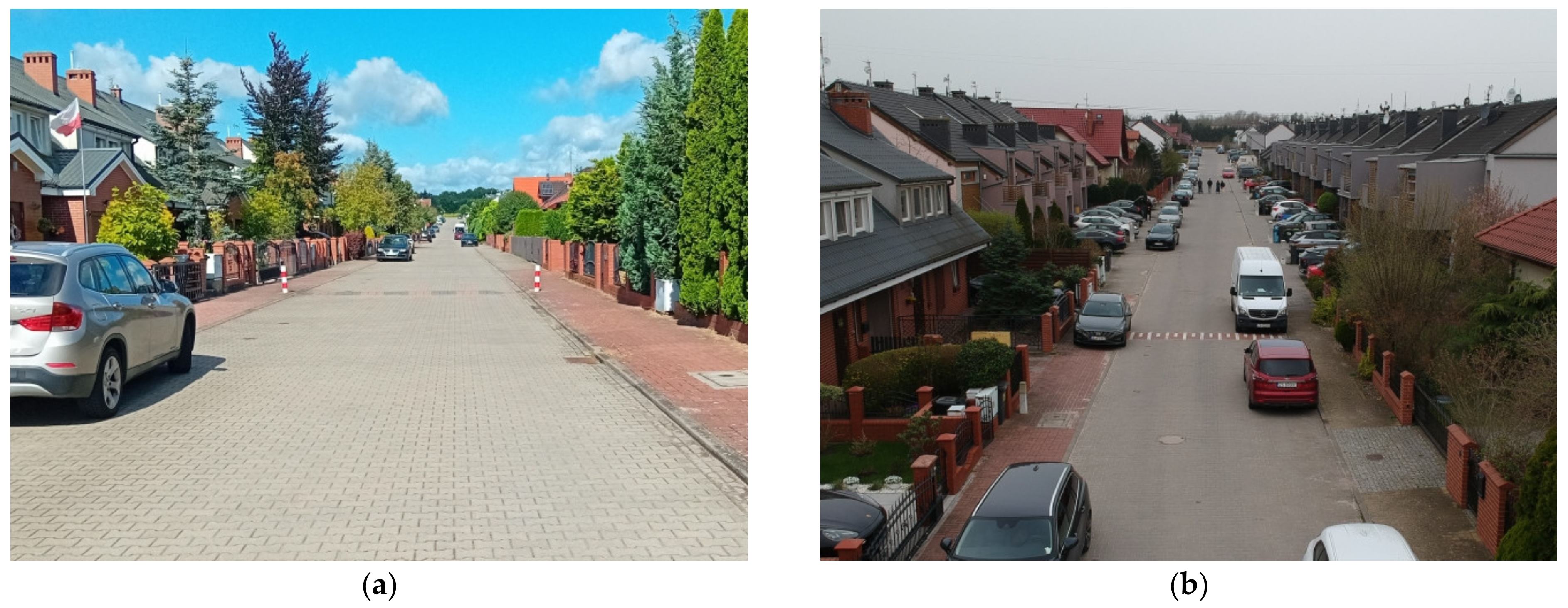
- Street surroundings on the approach to the home zone (houses on both or only one side of the street, presence of as yet empty building plots, and continuation with a paved street or unpaved forest road).
5. Selection of the Relevant Street Landscaping Characteristics Around the Analyzed Humps
- –
- Location of planned garages and private entryways;
- –
- Number of residents of a given single property, having determined the possible need for several parking spaces;
- –
- Planned front gardens or parking spaces in front of the house, perpendicular to the roadway axis (Figure 19b).
6. Discussion
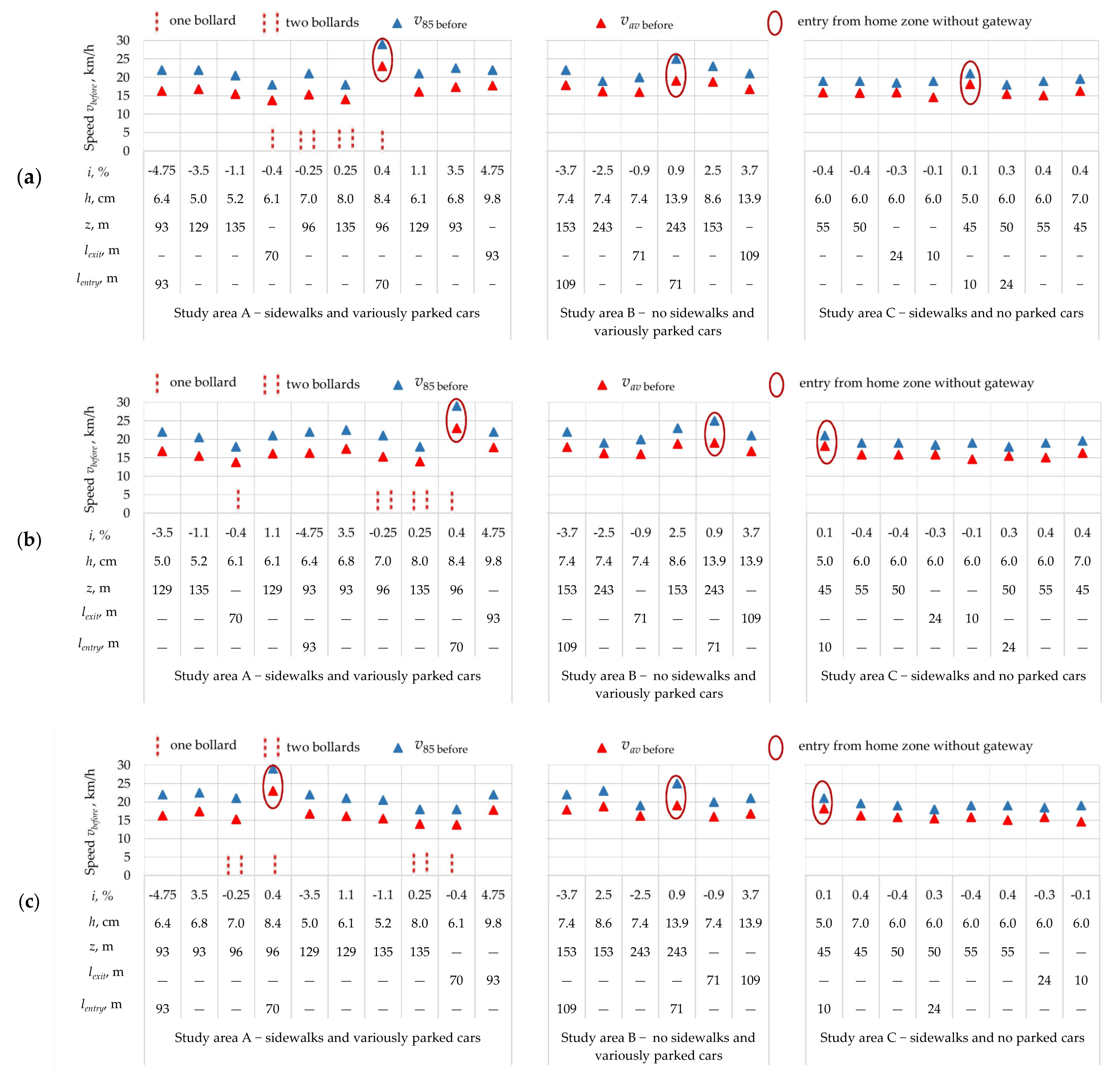
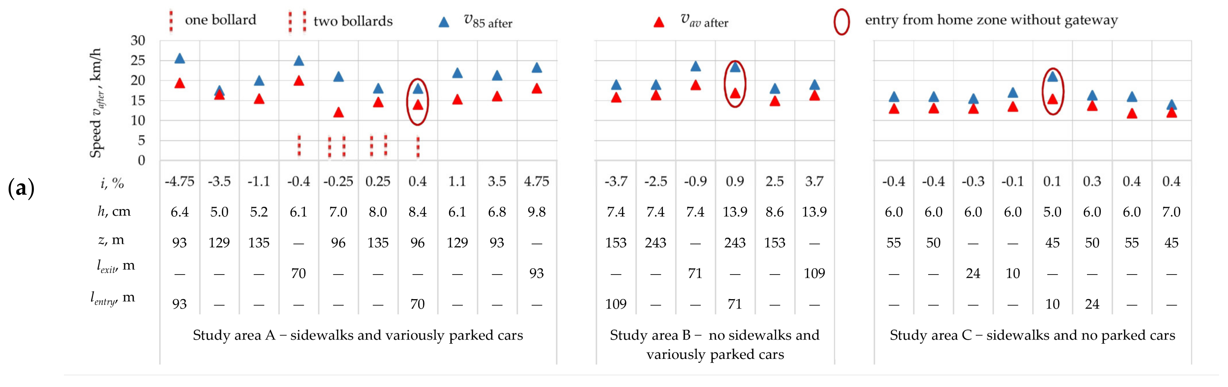
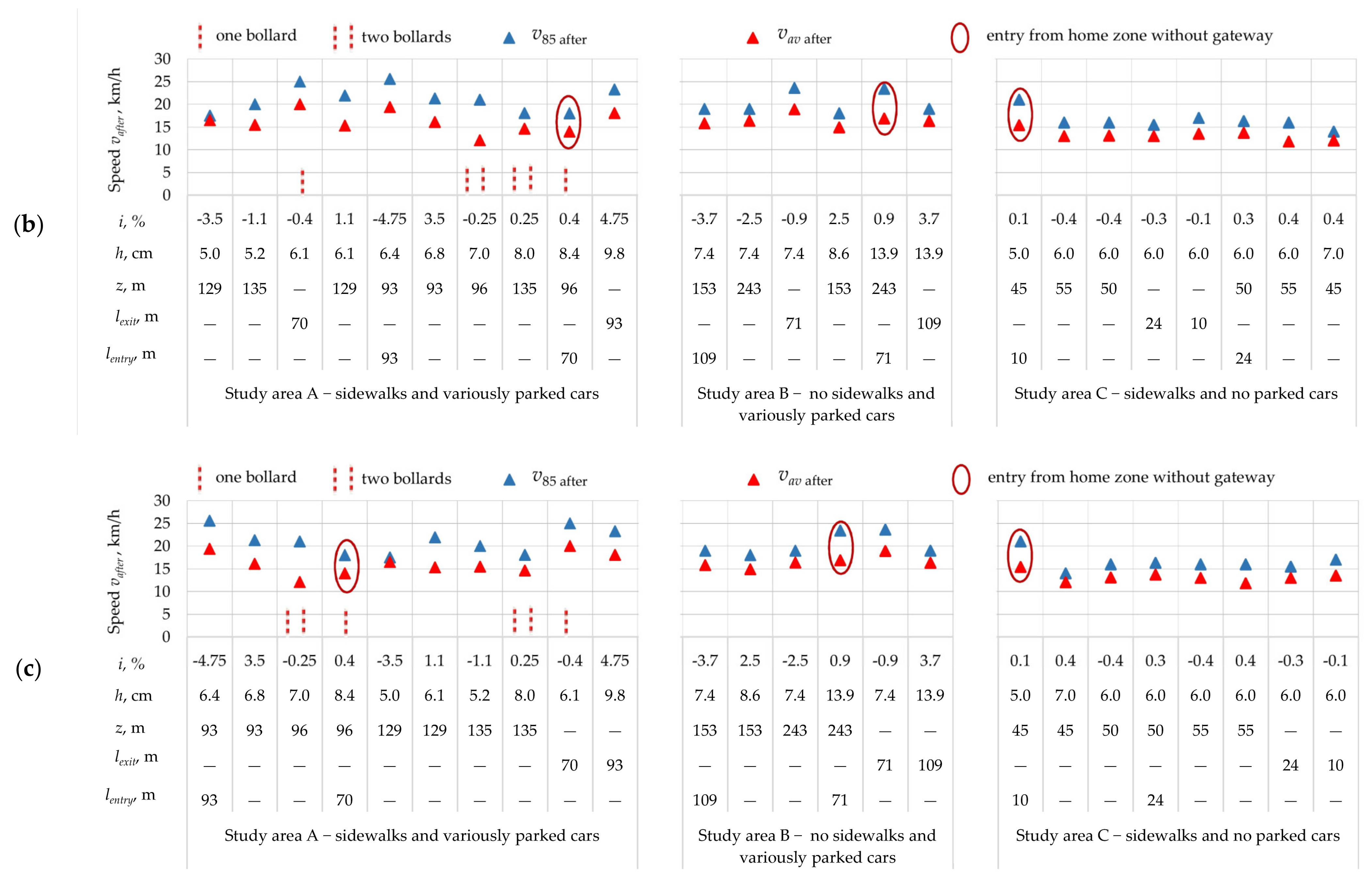
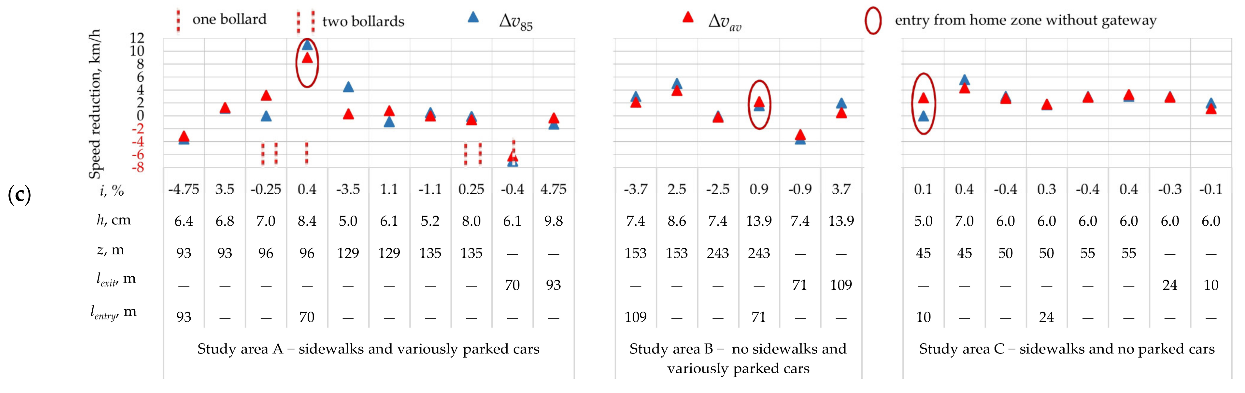
6.1. Analysis of the Influence of Selected Geometric Parameters of the Street and of the Humps Located Thereon on Speed
6.2. Analysis of the Effects of Other Factors
- –
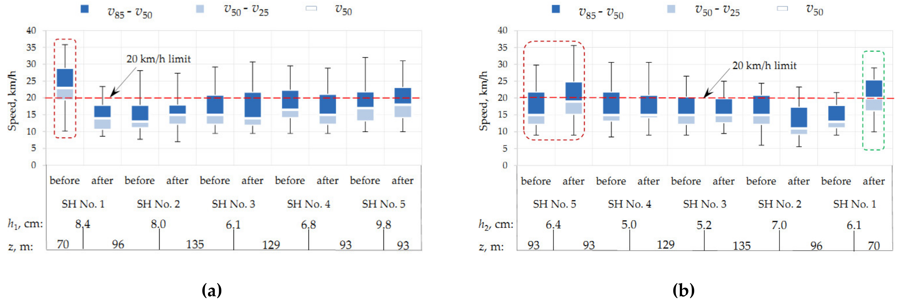
- In almost all study areas, “after” speeds were kept at about 20 km/h or less (Figure 22).
- –
- –
- In the traffic calming design process, particular attention should be paid to the first and the last road humps on a given street, and the right hump parameters should be chosen, taking into account the narrowing of the entrance and exit widths and the characteristics of street landscaping around them (Figure 21). We recommend using a gateway at the entrance and exit to/from the home zone.
- –
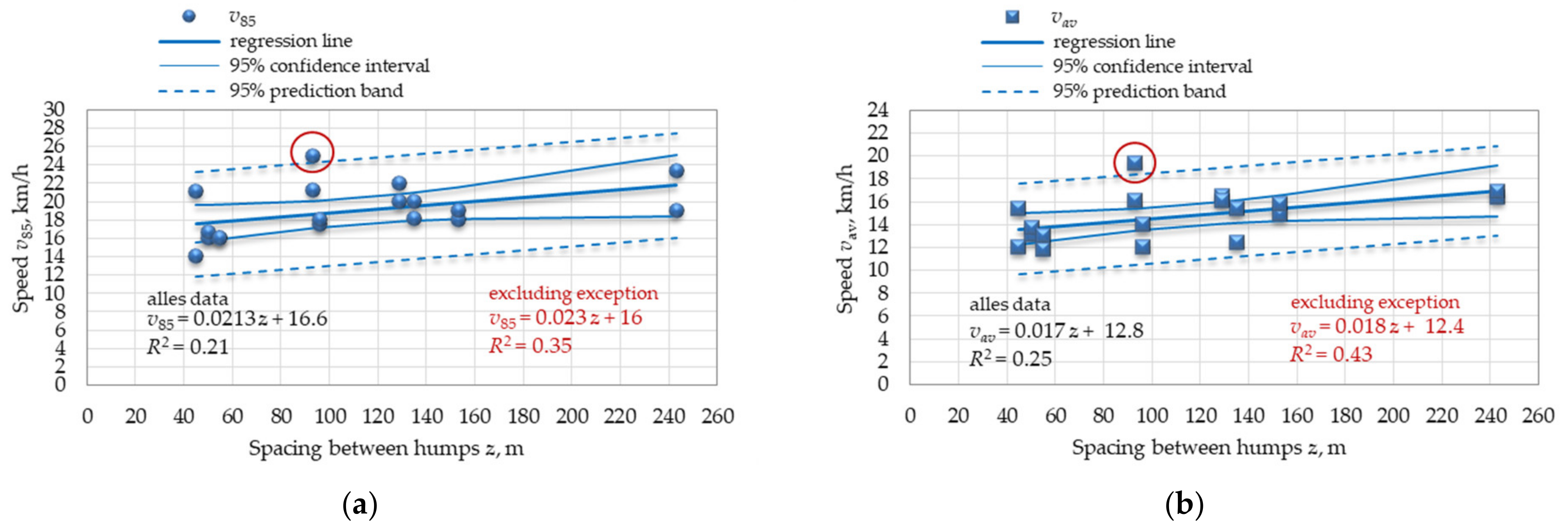
- “After” speeds depend not only on the hump height and hump spacing intervals but also on the street landscaping characteristics. The more these features are taken into account, the lower the v85 and vav speeds (Figure 22).
- –
7. Conclusions
- –
- The use of road humps in home zones is effective, and they contribute to keeping the speed limits by motorists, yet the slowing effect of the installed road humps depends on many factors.
- –
- The most effective in reducing traffic speeds are road humps with very steep ramps installed at 45 to 55 m spacing intervals.
- –
- The effectiveness of speed reductions on the sections between successive road humps depends primarily on the humps’ type(s), their geometric parameters and spacing interval(s), their location relative to the beginning or end of the street, and the direction of traffic, and last but not least, on the street gradient.
- –
- Other highly relevant factors include street landscaping features, i.e., sidewalks, hedges, bollards, and the parking arrangement in the vicinity of road humps. If there are no sidewalks, fences, hedges, and parked cars on the analyzed street located in a home zone, the effect of the installed road humps on the traffic speed may drop to a minimum, and this being so, the objective of road hump installations may not be achieved at all.
Author Contributions
Funding
Institutional Review Board Statement
Informed Consent Statement
Data Availability Statement
Conflicts of Interest
References
- Traffic Calming; Local Transport Note 1/07; Department for Regional Development (Northern Ireland), Scottish Executives, Welsh Assembly Government: London, UK, 2007.
- Richtlijn Verkeersdrempels. Publicatie 172; CROW: Ede, The Netherlands, 2002.
- Danish Road Directorate. Urban Traffic Areas—Part 7—Speed Reducers; Vejdirektoratet-Vejregeludvalget, Road Data Laboratory: Copenhagen, Denmark, 1991. [Google Scholar]
- Directives for the Design of Urban Roads; RASt 06; Road and Transportation Research Association: Köln, Germany, 2012.
- Ustawa—Prawo o ruchu drogowym, Dziennik Ustaw 1997 nr 98 poz. 602, z późn. zm. Available online: https://isap.sejm.gov.pl/isap.nsf/DocDetails.xsp?id=wdu19970980602 (accessed on 2 November 2024). (In Polish)
- Szczegółowe warunki techniczne dla znaków i sygnałów drogowych oraz urządzeń bezpieczeństwa ruchu drogowego i warunki ich umieszczania na drogach, Dziennik Ustaw 2021 poz. 2066. Available online: https://isap.sejm.gov.pl/isap.nsf/download.xsp/WDU20210002066/O/D20212066.pdf (accessed on 2 November 2024). (In Polish)
- Traffic Management Guidelines; Government Publications Sale Office, Sun Alliance House: Dublin, Ireland, 2014.
- Hummel, T.; Mackie, A.; Wells, P. Traffic Calming Measures in Built-Up Areas Literature Review PR/SE/622/02; Unpublished Project Report; Swedish National Road Administration: Borlänge, Sweden, 2002.
- Janssens, I.; Chalanton, I.; Bertrand, P.-J.; Caelen, E.; Broeckaert, M.; Dullaert, I.; Englebin, Y.; Houdmont, A.; Mathieu, V.; Temmerman, P.; et al. Het (Woon) Erf, Brochure ter Attentie van de Weg Beheerders; Belgisch Institut voor de Verkeersveiligheid BIVV: Brussel, Belgium, 2013. [Google Scholar]
- DDOT. Guidelines on Vertical Traffic Calming Implementation; District Departament of Transportation DDOT: Washington, DC, USA, 2022.
- Sayer, I.A.; Nicholls, D.A.; Layfield, R.E. Traffic Calming: Passenger and Rider Discomfort at Sinusoidal, Round-Top and Flat-Top Humps—a Track Trial at TRL, Report 417; Department of the Environment, Transport and the Regions: Crowthorne, UK, 1999.
- Webster, D.C.; Layfield, R.E. Traffic Calming—Road Hump Schemes Using 75 Mm High Humps, Report 186; Transport Research Laboratory: Crowthorne, UK, 1996. [Google Scholar]
- Watts, G.R. Road Humps for the Control of Vehicle Speeds; TRRL Laboratory Report 597; Transport Research Laboratory: Crowthorne, UK, 1973. [Google Scholar]
- Watts, G.R.; Harris, G.J. Traffic Calming: Vehicle Generated Ground-Borne Vibration Alongside Speed Control Cushions and Road Humps; TRL Report 235; Transport Research Laboratory: Crowthorne, UK, 1996. [Google Scholar]
- Webster, D.C. Road Humps for Controlling Vehicle Speeds; TRL Project Report 18; Transport Research Laboratory: Crowthorne, UK, 1993. [Google Scholar]
- Webster, D.C. The grounding of vehicles on road humps. Traffic Eng. Control. 1993, 34, 369–371. [Google Scholar]
- Webster, D.C. Speeds at ‘Thumps’ and Low Height Road Humps; TRL Project Report 101; Transport Research Laboratory: Crowthorne, UK, 1994. [Google Scholar]
- CROW Gerelateerde Verkeersdrempels &–Plateaus; Struyk Verwo–INFRA–Straatbepland: Ede, The Netherlands, 2002.
- Pau, M. Speed Bumps May Induce Improper Drivers’ Behavior: Case Study in Italy. J. Transp. Eng. 2002, 128, 472–478. [Google Scholar] [CrossRef]
- Pau, M.; Angius, S. Do speed bumps really decrease traffic speed? An Italian experience. Accid. Anal. Prev. 2001, 33, 585–597. [Google Scholar] [CrossRef] [PubMed]
- Benzaman, B.; Ward, N.J.; Schell, W.J. The Influence of Inferred Traffic Safety Culture on Traffic Safety Performance in U.S. States (1994–2014). J. Saf. Res. 2022, 80, 311–319. [Google Scholar] [CrossRef] [PubMed]
- Zaidel, D.; Hakkert, A.S.; Pistiner, A.H. The use of road humps for moderating speeds on urban streets. Accid. Anal. Prev. 1992, 24, 45–56. [Google Scholar] [CrossRef]
- Gitelman, V.; Carmel, R.; Pesahov, F.; Chen, S. Changes in road-user behaviors following the installation of raised pedestrian crosswalks combined with preceding speed humps, on urban arterials. Transp. Res. Part F Traffic Psychol. Behav. 2017, 46, 356–372. [Google Scholar] [CrossRef]
- Antić, B.; Pešić, D.; Vujanić, M.; Lipovac, K. The influence of speed bumps heights to the decrease of the vehicle speed—Belgrade experience. Saf. Sci. 2013, 57, 303–312. [Google Scholar] [CrossRef]
- Gedik, A.; Bilgin, E.; Lav, A.H.; Artan, R. An Investigation into the Effect of Parabolic Speed Hump Profiles on Ride Comfort and Driving Safety under Variable Vehicle Speeds: A Campus Experience. Sustain. Cities Soc. 2019, 45, 413–421. [Google Scholar] [CrossRef]
- Kassem, E.; Al-Nassar, Y. Dynamic Considerations of Speed Control Humps. Transp. Res. Part B Methodol. 1982, 16, 291–302. [Google Scholar] [CrossRef]
- Khorshid, E.; Alkalby, F.; Kamal, H. Measurement of whole-body vibration exposure from speed control humps. J. Sound Vib. 2007, 304, 640–659. [Google Scholar] [CrossRef]
- Loprencipe, G.; Moretti, L.; Pantuso, A.; Banfi, E. Raised Pedestrian Crossings: Analysis of Their Characteristics on a Road Network and Geometric Sizing Proposal. Appl. Sci. 2019, 9, 2844. [Google Scholar] [CrossRef]
- D’Apuzzo, M.; Evangelisti, A.; Santilli, D.; Nardoianni, S.; Cappelli, G.; Nicolosi, V. Towards a New Design Methodology for Vertical Traffic Calming Devices. Sustainability 2023, 15, 13381. [Google Scholar] [CrossRef]
- Majer, S.; Sołowczuk, A.; Kurnatowski, M. Design and Construction Aspects of Concrete Block Paved Vertical Traffic-Calming Devices Located in Home Zone Areas. Sustainability 2024, 16, 2982. [Google Scholar] [CrossRef]
- Jarvis, J.R.; Sweatman, P.F. The Loading of Pavements in the Vicinity of Road Humps. Aust. Road Res. 1982, 11, 45–55. [Google Scholar]
- Zakaria, M.H.; Al-Ayaat, A.H.; Shwaly, S.A. Impact of Road Humps on the Pavement Surface Condition. Civ. Eng. J. 2019, 5, 1314–1326. [Google Scholar] [CrossRef]
- Radhiah Bachok, K.S.; Kadar Hamsa, A.A.; Bin Mohamed, M.Z.; Ibrahim, M. A Theoretical Overview of Road Hump Effects on Traffic Noise in Improving Residential Well-Being. Transp. Res. Procedia 2017, 25, 3383–3397. [Google Scholar] [CrossRef]
- Wewalwala, S.; Sonnadara, U. Traffic Noise Enhancement Due to Speed Bumps. Sri Lankan J. Phys. 2012, 12, 1–6. [Google Scholar] [CrossRef]
- Rosli, N.S.; Hamsa, A.A.K. Evaluating the Effects of Road Hump on Traffic Volume and Noise Level at Taman Keramat Residential Area, Kuala Lumpur. J. East. Asia Soc. Transp. Stud. 2013, 10, 1171–1188. [Google Scholar] [CrossRef]
- Lee, G.; Joo, S.; Oh, C.; Choi, K. An evaluation framework for traffic calming measures in residential areas. Transp. Res. Part D Transp. Environ. 2013, 25, 68–76. [Google Scholar] [CrossRef]
- Gonzalo-Orden, H.; Pérez-Acebo, H.; Unamunzaga, A.L.; Arce, M.R. Effects of Traffic Calming Measures in Different Urban Areas. Transp. Res. Procedia 2018, 33, 83–90. [Google Scholar] [CrossRef]
- Yeo, I.; Baek, J.-G.; Choi, J.-W.; Kim, Y.S. The Optimal Spacing of Speed Humps in Traffic Calming Areas. J. Korean Soc. Road Eng. 2013, 15, 151–157. [Google Scholar] [CrossRef]
- Kveladze, I.; Agerholm, N. Visual Analysis of Speed Bumps Using Floating Car Dataset. J. Locat. Based Serv. 2018, 12, 119–139. [Google Scholar] [CrossRef]
- Vitronic. Speed Displays Traffic Detection, Radar, Detection, Software; Vitronic: Kędzierzyn Koźle, Poland, 2015. [Google Scholar]
- Majer, S.; Sołowczuk, A. Traffic Circle–An Example of Sustainable Home Zone Design. Sustainability 2023, 15, 16751. [Google Scholar] [CrossRef]


| ST No. | v85 before | v85 after | ∆v85 | vav before | vav after | ∆vav | Equation (1) | Equation (2) | |
|---|---|---|---|---|---|---|---|---|---|
| Before | After | ||||||||
| Direction of traffic—from east | |||||||||
| 1 | 29.0 | 18.0 | 11.0 | 23.0 | 14.0 | 9.0 | 0.33 | 0.92 | 4.27 (1) |
| 2 | 18.0 | 18.1 | −0.1 | 14.0 | 14.6 | −0.7 | 0.73 | 0.53 | 1.03 |
| 3 | 21.0 | 21.9 | −0.9 | 16.1 | 15.3 | 0.8 | 0.78 | 1.04 | 0.82 |
| 4 | 22.5 | 21.3 | 1.2 | 17.4 | 16.1 | 1.3 | 0.43 | 0.66 | 0.83 |
| 5 | 22.0 | 23.3 | −1.3 | 17.8 | 18.1 | −0.3 | 0.72 | 0.47 | 0.50 |
| Direction of traffic—from west | |||||||||
| 5 | 22.0 | 25.0 | −3.0 | 16.3 | 19.4 | −3.1 | 0.99 | 0.51 | 1.99 |
| 4 | 22.0 | 21.0 | 1.0 | 16.8 | 16.5 | 0.2 | 0.55 | 0.81 | 0.71 |
| 3 | 20.5 | 20.0 | 0.5 | 15.5 | 15.5 | 0.1 | 0.89 | 0.60 | 0.50 |
| 2 | 21.0 | 17.5 | 3.5 | 15.3 | 12.1 | 3.2 | 0.51 | 0.59 | 1.97 |
| 1 | 18.0 | 25.6 | −7.6 | 13.8 | 20.0 | −6.2 | 0.53 | 0.88 | 2.80 |
| ST No. | v85 before | v85 after | ∆v85 | vav before | vav after | ∆vav | Equation (1) | Equation (2) | |
|---|---|---|---|---|---|---|---|---|---|
| Before | After | ||||||||
| Direction of traffic—from east | |||||||||
| 1 | 25.0 | 23.4 | 1.6 | 19.1 | 16.9 | 2.2 | 0.40 | 0.37 | 1.20 |
| 2 | 23.0 | 18.0 | 5.0 | 18.8 | 14.9 | 3.9 | 0.64 | 1.06 | 0.72 |
| 3 | 21.0 | 19.0 | 2.0 | 16.8 | 16.3 | 0.5 | 0.79 | 0.58 | 0.99 |
| Direction of traffic—from west | |||||||||
| 3 | 22.0 | 19.0 | 3.0 | 17.9 | 15.8 | 2.1 | 0.54 | 0.36 | 0.64 |
| 2 | 19.0 | 19.0 | 0.0 | 16.2 | 16.4 | −0.2 | 0.66 | 0.63 | 1.99 (1) |
| 1 | 20.0 | 23.6 | −3.6 | 16.0 | 18.9 | −2.9 | 0.76 | 0.46 | 1.23 |
| ST No. | v85 before | v85 after | ∆v85 | vav before | vav after | ∆vav | Equation (1) | Equation (2) | |
|---|---|---|---|---|---|---|---|---|---|
| Before | After | ||||||||
| Direction of traffic—from east | |||||||||
| 1 | 21.0 | 21.0 | 0.0 | 18.2 | 15.4 | 2.8 | 1.17 | 1.35 | 2.01 (1) |
| 2 | 19.0 | 16.0 | 3.0 | 15.9 | 13.0 | 2.9 | 1.35 | 0.82 | 2.50 |
| 3 | 19.0 | 16.0 | 3.0 | 15.8 | 13.1 | 2.7 | 1.15 | 1.21 | 2.50 |
| 4 | 18.5 | 15.5 | 3.0 | 15.9 | 13.0 | 2.8 | 0.64 | 0.52 | 2.66 |
| Direction of traffic—from west | |||||||||
| 4 | 18.0 | 16.3 | 1.7 | 15.5 | 13.7 | 1.7 | 0.56 | 0.58 | 2.10 |
| 3 | 19.0 | 16.0 | 3.0 | 15.1 | 11.8 | 3.3 | 0.48 | 0.48 | 2.50 |
| 2 | 19.6 | 14.0 | 5.6 | 16.3 | 12.0 | 4.3 | 0.62 | 0.72 | 3.55 |
| 1 | 19.0 | 17.0 | 2.0 | 14.6 | 13.5 | 1.1 | 0.70 | 0.70 | 1.13 |
| SH No. | Two-Sample K–S Test | Test of Independence | Median Test | |||
|---|---|---|---|---|---|---|
| Before Hump | After Hump | Before Hump | After Hump | Before Hump | After Hump | |
| Equation (3a) | Equation (3b) | Equation (4a) | Equation (4b) | Equation (5a) | Equation (5b) | |
| Study area A | ||||||
| 1 | 3.56 (1) | 3.18 | 41.55 | 32.82 | 35.6 | 34.5 |
| 2 | 0.89 (2) | 1.91 | 3.05 | 0.67 | 5.5 | 5.5 |
| 3 | 0.34 | 0.82 | 0.16 (3) | 0.49 | 2.5 | 3.4 |
| 4 | 0.67 | 0.88 | 0.01 | 0.01 | 2.5 | 3.9 |
| 5 | 1.31 | 1.00 | 4.50 | 4.22 | 7.7 | 5.9 |
| Study area B | ||||||
| 1 | 1.58 | 1.04 | 12.87 | 0.15 | 22.6 | 11.3 |
| 2 | 1.47 | 1.65 | 9.29 | 2.84 | 19.3 | 7.4 |
| 3 | 0.62 | 0.45 | 0.64 | 0.26 | 15.8 | 15.2 |
| Study area C | ||||||
| 1 | 2.82 | 1.69 | 6.66 | 2.94 | 43.9 | 12.9 |
| 2 | 0.56 | 1.29 | 5.78 | – (4) | 0.80 | 9.13 |
| 3 | 1.05 | 2.26 | 0.00 | – | 9.36 | 22.9 |
| 4 | 0.40 | 0.64 | 3.74 | – | 0.2 | 0.9 |
| SHs Nos. i and i + 1 | Two-Sample K-S Test | Test of Independence | Median Test | |||
|---|---|---|---|---|---|---|
| Before Hump | After Hump | Before Hump | After Hump | Before Hump | After Hump | |
| Equation (6a) | Equation (6b) | Equation (7a) | Equation (7b) | Equation (8a) | Equation (8b) | |
| Study area A—from east | ||||||
| 1 & 2 | 4.47 (1) | 0.98 (2) | 64.44 | 0.89 | 76.9 | 0.88 |
| 2 & 3 | 1.21 | 0.80 | 4.01 | 1.56 | 7.71 | 3.43 |
| 3 & 4 | 0.97 | 0.72 | 0.13 (3) | 0.01 | 10.84 | 7.45 |
| 4 & 5 | 0.65 | 1.13 | 2.02 | 2.71 | 3.42 | 4.28 |
| Study area A—from west | ||||||
| 5 & 4 | 0.54 | 1.66 | 0.00 | 10.97 | 4.88 | 6.58 |
| 4 & 3 | 0.69 | 0.68 | 0.44 | 0.49 | 2.33 | 2.63 |
| 3 & 2 | 0.47 | 1.96 | 0.02 | 1.56 | 1.57 | 3.68 |
| 2 & 1 | 1.01 | 3.47 | 2.62 | 30.05 | 8.37 | 34.98 |
| Study area B—from east | ||||||
| 1 & 2 | 0.60 | 0.96 | 0.54 | 2.43 | 11.29 | 8.39 |
| 2 & 3 | 0.82 | 0.74 | 1.81 | 0.12 | 15.82 | 20.78 |
| Study area B—from west | ||||||
| 3 & 2 | 1.11 | 1.23 | 3.96 | 0.37 | 3.18 | 4.72 |
| 2 & 1 | 2.54 | 2.48 | 1.45 | 2.98 | 13.09 | 8.42 |
| Study area C—from east | ||||||
| 1 & 2 | 1.85 | 2.34 | 18.82 | 14.20 | 26.5 | 14.1 |
| 2 & 3 | 0.56 | 0.73 | 4.75 | – (4) | 1.74 | 0.51 |
| 3 & 4 | 0.40 | 0.73 | 0.08 | – | 0.55 | 0.12 |
| Study area C—from west | ||||||
| 4 & 3 | 0.89 | 2.42 | 4.75 | – | 0.35 | 19.57 |
| 3 & 2 | 1.21 | 0.97 | 0.07 | – | 1.32 | 1.36 |
| 2 & 1 | 1.37 | 1.21 | 0.07 | 6.24 | 9.13 | 4.85 |
| Hump No. | Street Landscaping Features Surrounding Humps | |||||
|---|---|---|---|---|---|---|
| a | b | c | d | e | f | |
| Study area A—from east | ||||||
| 1 | 1 | 0 | 0 | 0 | 1 | 1 |
| 2 | 1 | 1 | 0 | 0.25 | 1 | 1 |
| 3 | 1 | 1 | 0 | 0.5 | 1 | 0 |
| 4 | 1 | 1 | 0 | 1 | 0.25 | 0 |
| 5 | 1 | 0 | 0 | 0.5 | 0.25 | 0 |
| Study area A—from west | ||||||
| 5 | 1 | 0 | 0 | 1 | 0.25 | 0 |
| 4 | 1 | 1 | 0 | 1 | 0.25 | 0 |
| 3 | 1 | 1 | 0 | 0.25 | 1 | 0 |
| 2 | 1 | 1 | 0 | 0 | 1 | 1 |
| 1 | 1 | 0 | 0 | 0 | 0.25 | 1 |
| Study area B—from east | ||||||
| 1 | 0 | 0 | 0 | 0.25 | 0 | 0 |
| 2 | 1 | 1 | 0 | 0.5 | 0.5 | 0 |
| 3 | 0 | 0 | 1 | 1 | 0 | 0 |
| Study area B—from west | ||||||
| 3 | 0 | 0 | 1 | 1 | 0 | 0 |
| 2 | 1 | 1 | 0 | 0.5 | 0.5 | 0 |
| 1 | 0 | 0 | 0 | 0.25 | 0 | 0 |
| Study area C—from east | ||||||
| 1 | 0 | 0 | 0 | 0 | 0 | 0 |
| 2 | 0 | 1 | 1 | 0 | 0 | 0 |
| 3 | 1 | 1 | 0 | 0 | 0 | 0 |
| 4 | 0 | 0 | 1 | 0 | 0 | 0 |
| Study area C—from west | ||||||
| 4 | 1 | 0 | 0 | 0 | 0 | 0 |
| 3 | 1 | 1 | 0 | 0 | 0 | 0 |
| 2 | 0.25 | 1 | 0 | 0 | 0 | 0 |
| 1 | 0.25 | 0 | 1 | 0 | 0 | 0 |
| Speed Parameters, km/h | Street Parameters or Hump Geometric Parameters | ||||
|---|---|---|---|---|---|
| Spacing Between Humps | Approach Ramp Height | Longitudinal Gradient of the Street Before Hump | Longitudinal Gradient of the Street After Hump | Approach Ramp Gradient | |
| Study area A | |||||
| v85 after | 0.65 | 0.21 | –0.15 | 0.02 | –0.36 |
| vav after | 0.87 | –0.05 | –0.24 | –0.10 | –0.53 |
| ∆v85 | –0.87 | 0.22 | 0.34 | 0.24 | 0.46 |
| ∆vav | −0.69 | 0.23 | 0.27 | 0.19 | 0.49 |
| Study area B | |||||
| v85 after | –0.13 | –0.16 | 0.02 | –0.18 | –0.09 |
| vav after | –0.05 | –0.10 | –0.03 | –0.26 | –0.02 |
| ∆v85 | –0.34 | 0.29 | 0.06 | 0.15 | 0.20 |
| ∆vav | −0.34 | 0.33 | 0.18 | 0.28 | 0.21 |
| Study area C | |||||
| v85 after | 0.44 | –0.93 | –0.03 | –0.03 | 0.23 |
| vav after | 0.62 | –0.82 | –0.19 | –0.19 | 0.18 |
| ∆v85 | –0.54 | 0.95 | 0.12 | 0.12 | –0.17 |
| ∆vav | −0.83 | 0.41 | 0.27 | 0.27 | 0.47 |
Disclaimer/Publisher’s Note: The statements, opinions and data contained in all publications are solely those of the individual author(s) and contributor(s) and not of MDPI and/or the editor(s). MDPI and/or the editor(s) disclaim responsibility for any injury to people or property resulting from any ideas, methods, instructions or products referred to in the content. |
© 2025 by the authors. Licensee MDPI, Basel, Switzerland. This article is an open access article distributed under the terms and conditions of the Creative Commons Attribution (CC BY) license (https://creativecommons.org/licenses/by/4.0/).
Share and Cite
Majer, S.; Sołowczuk, A. Effectiveness of a Series of Road Humps on Home Zone Streets: A Case Study. Sustainability 2025, 17, 644. https://doi.org/10.3390/su17020644
Majer S, Sołowczuk A. Effectiveness of a Series of Road Humps on Home Zone Streets: A Case Study. Sustainability. 2025; 17(2):644. https://doi.org/10.3390/su17020644
Chicago/Turabian StyleMajer, Stanisław, and Alicja Sołowczuk. 2025. "Effectiveness of a Series of Road Humps on Home Zone Streets: A Case Study" Sustainability 17, no. 2: 644. https://doi.org/10.3390/su17020644
APA StyleMajer, S., & Sołowczuk, A. (2025). Effectiveness of a Series of Road Humps on Home Zone Streets: A Case Study. Sustainability, 17(2), 644. https://doi.org/10.3390/su17020644