
Computational Fluid Dynamics (CFD) Technology Methodology and Analysis of Waste Heat Recovery from High-Temperature Solid Granule: A Review

 ,
,  ,
, 

Abstract
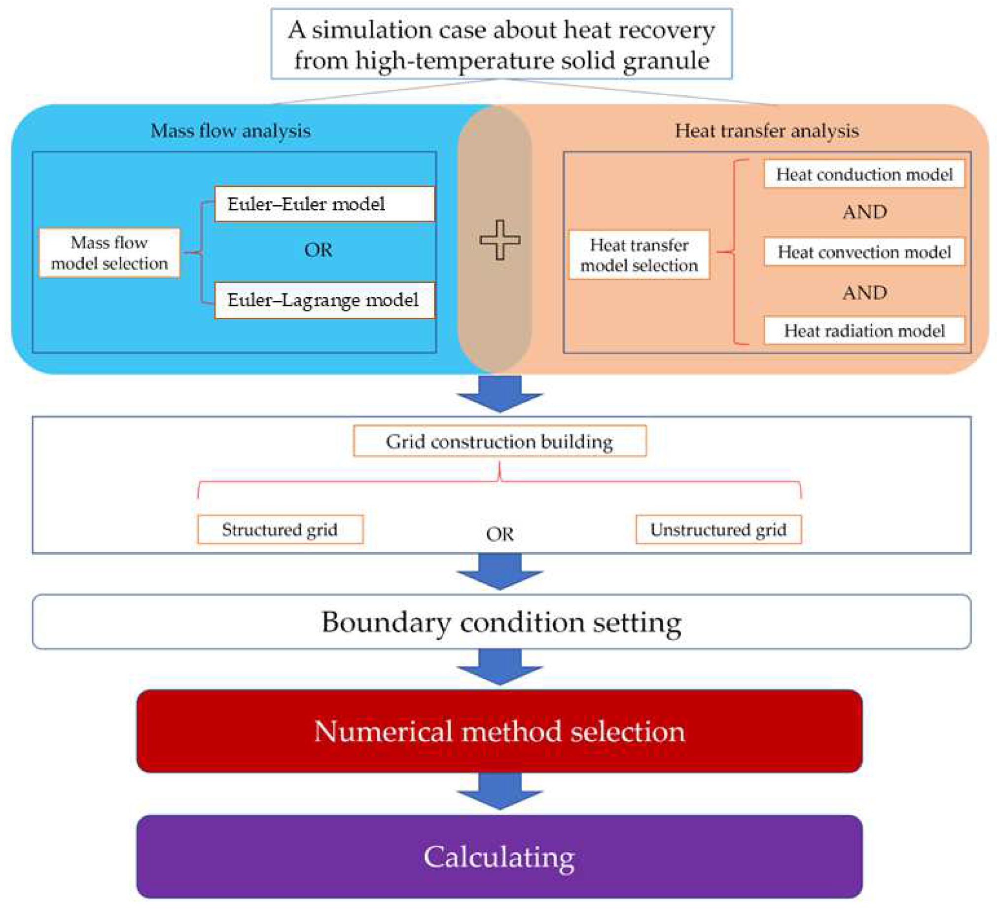
1. Introduction
2. Computer Fluid Dynamics (CFD) Method and CFD Coupling Method
3. Mass Flow Analysis
3.1. Solve Model Selecting
3.1.1. Two Fluids Method
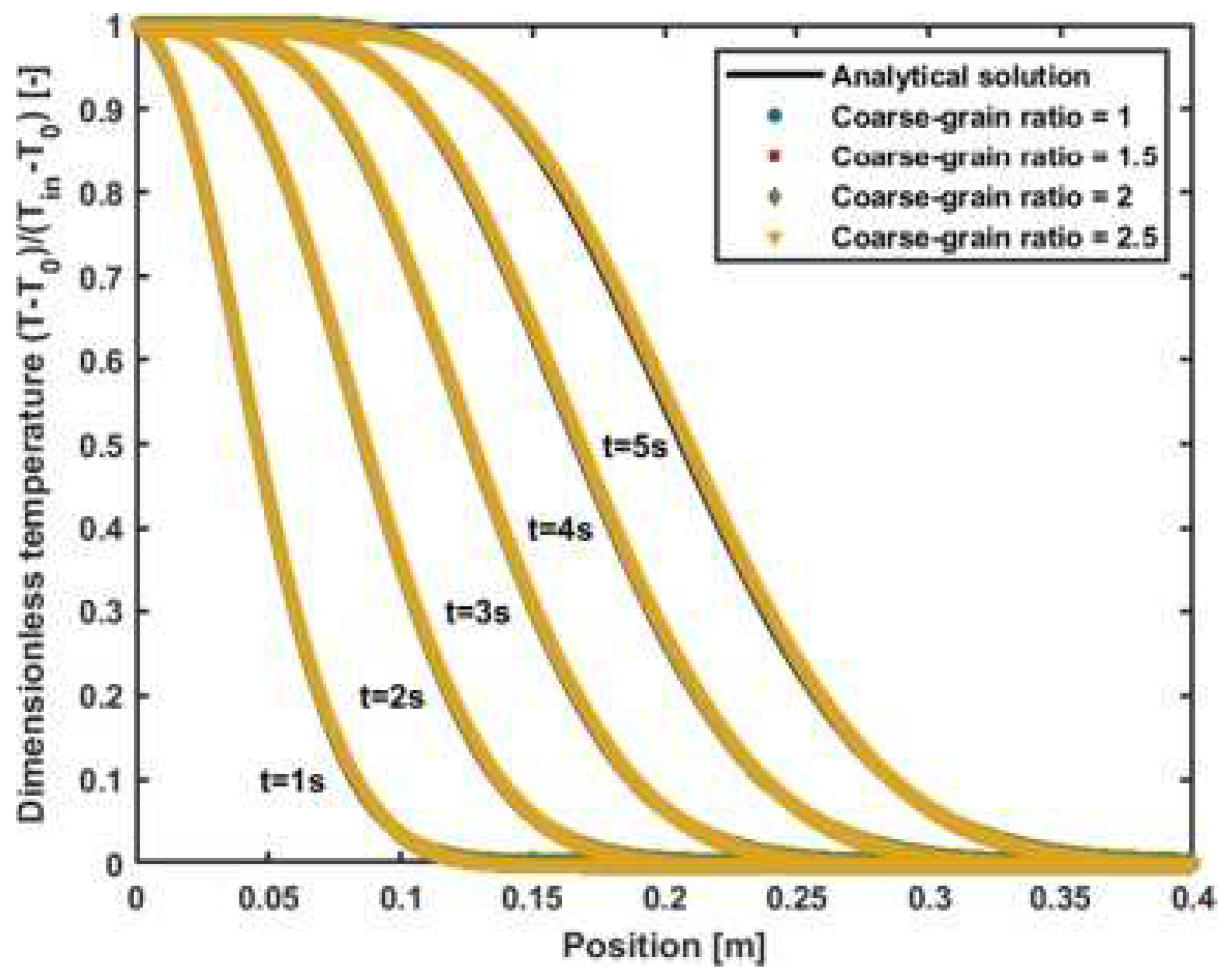
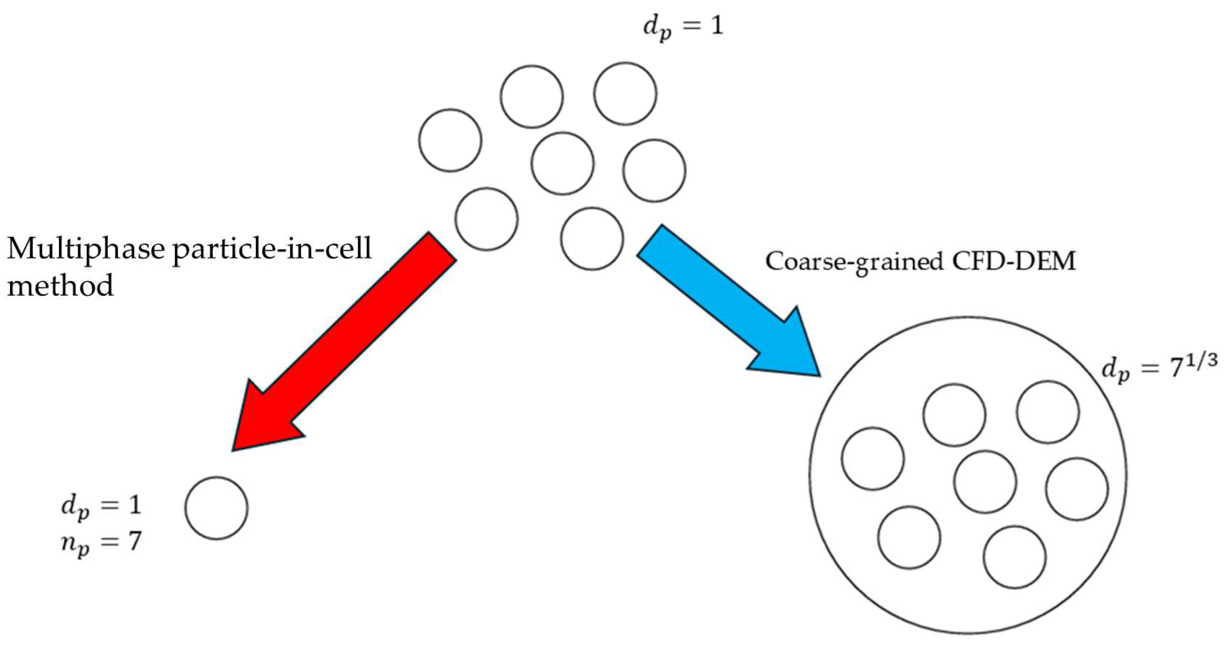
3.1.2. CFD–Discrete Element Method
3.1.3. Direct Numerical Simulation Method
3.1.4. Multiphase Particle-in-Cell Method
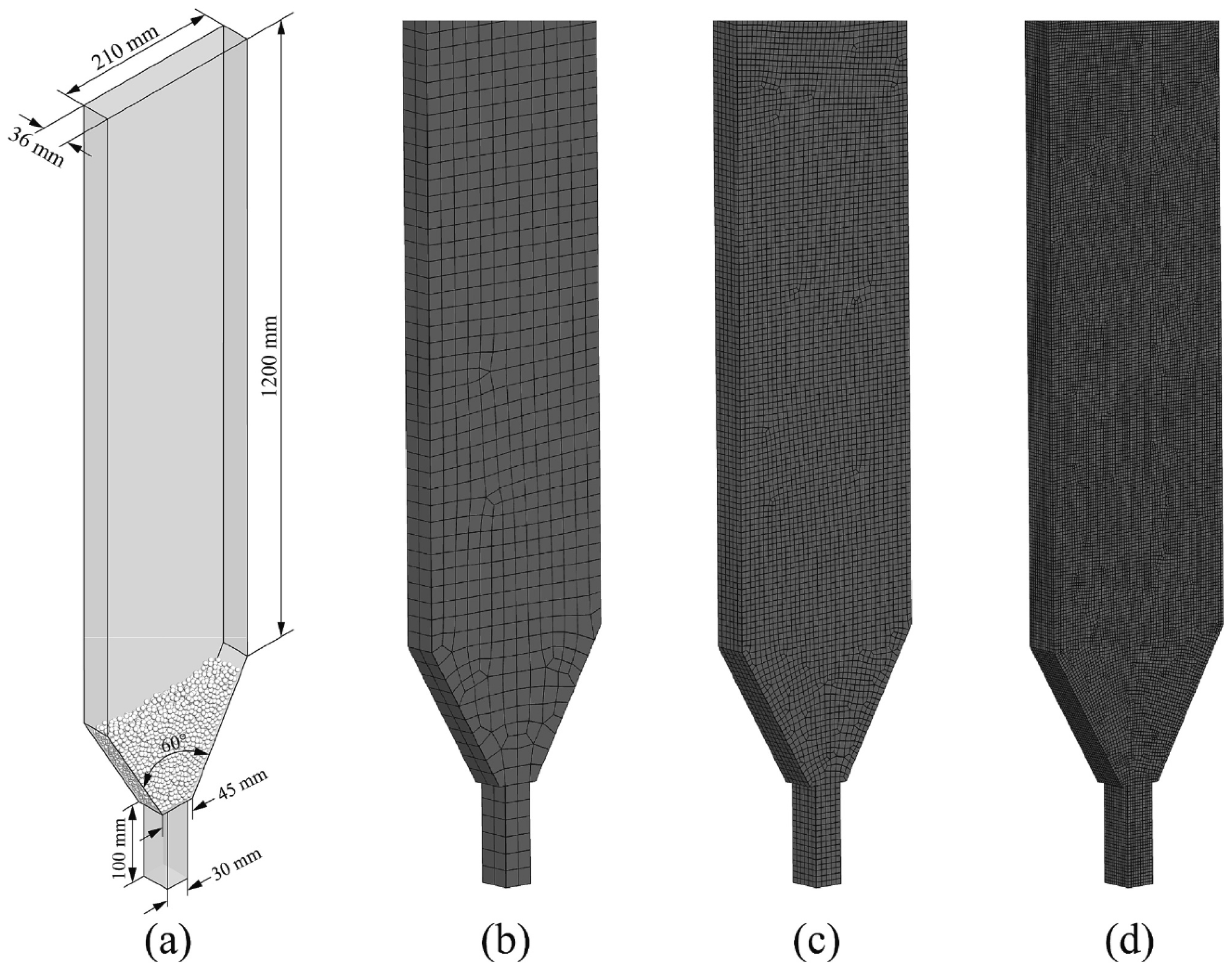
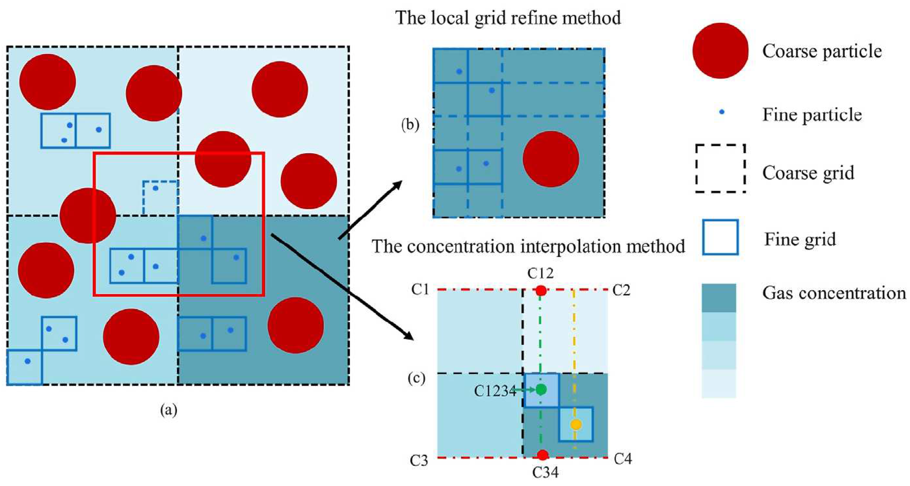
3.2. Grid (Mesh) Building
4. Heat Transfer Analysis
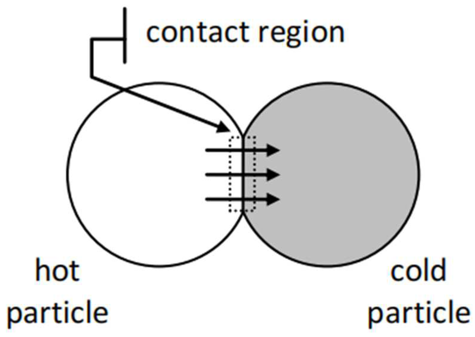
4.1. Particle-Scale Heat Conduction
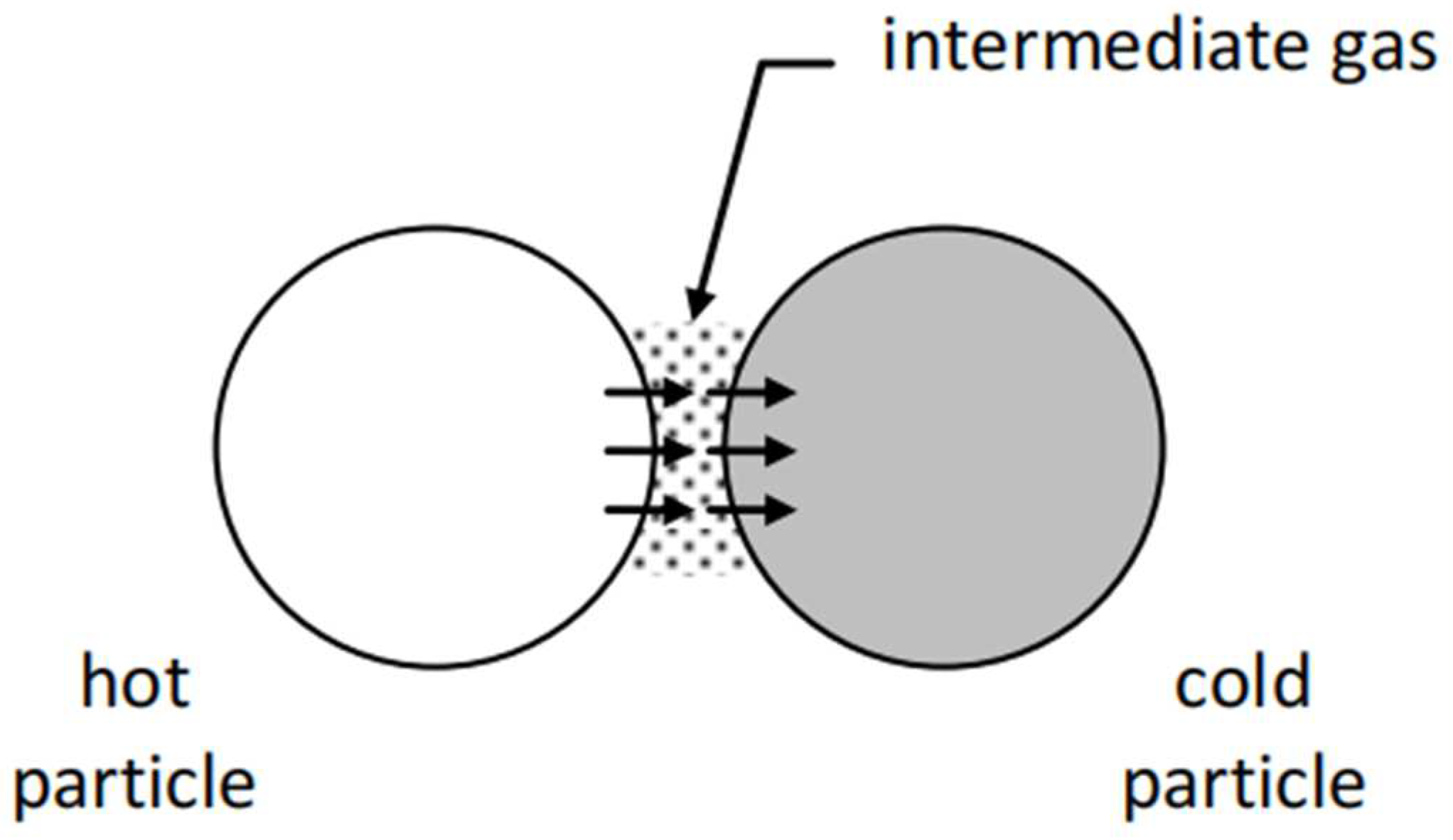
4.2. Particle-Scale Heat Convection
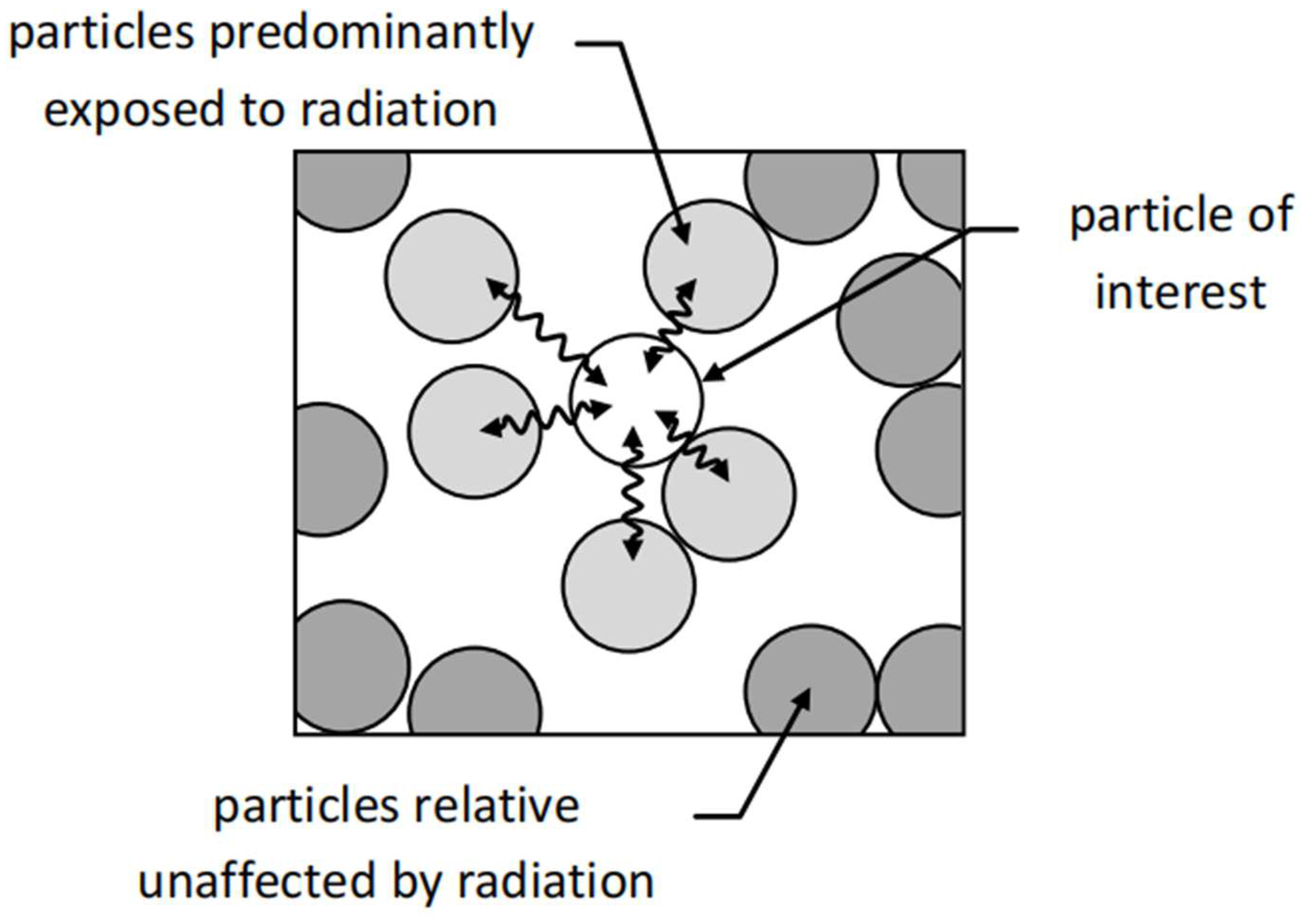
4.3. Particle-Scale Heat Radiation
5. Summary and Prospects
5.1. Summary
5.2. Prospects
5.2.1. More Precise Physical Model and Empirical Formula
5.2.2. More Suitable Grid Construction for Larger-Scale Simulation as Real Industrial Processes
5.2.3. More Diverse CFD Methods and CFD Coupling Methods for Solving the Problems
5.2.4. Other Advanced Technology Development Used in CFD Methods and CFD Coupling Methods
Author Contributions
Funding
Institutional Review Board Statement
Informed Consent Statement
Data Availability Statement
Conflicts of Interest
References
- Vizitiu Ștefănica, E.; Abid, C.; Burlacu, A.; Vizitiu, R. Ștefan; Balan, M.C. Strategic Optimization of Operational Parameters in a Low-Temperature Waste Heat Recovery System: A Numerical Approach. Sustainability 2024, 16, 7013. [Google Scholar] [CrossRef]
- Vizitiu, R.Ș.; Vizitiu Ștefănica, E.; Burlacu, A.; Abid, C.; Balan, M.C.; Kaba, N.E. Experimental Investigation of a Water–Air Heat Recovery System. Sustainability 2024, 16, 7686. [Google Scholar] [CrossRef]
- Zhang, H.; Wang, H.; Zhu, X.; Qiu, Y.J.; Li, K.; Chen, R.; Liao, Q. A Review of Waste Heat Recovery Technologies towards Molten Slag in Steel Industry. Appl. Energy 2013, 112, 956–966. [Google Scholar] [CrossRef]
- Available online: https://www.stats.gov.cn/sj/zxfb/202402/t20240228_1947915.html (accessed on 11 November 2024).
- Bisio, G.; Rubatto, G. Energy Saving and Some Environment Improvements in Coke-Oven Plants. Energy 2000, 25, 247–265. [Google Scholar] [CrossRef]
- Gao, H.; Liu, Y.; Zheng, B.; Sun, P.; Lu, M.; Yin, Q. Modeling of Fractal Heat Conduction of Semi-Coke Bed in Waste Heat Recovery Steam Generator for Hydrogen Production. Int. J. Hydrogen Energy 2019, 44, 25240–25247. [Google Scholar] [CrossRef]
- Liu, J.; Yu, Q.; Peng, J.; Hu, X.; Duan, W. Thermal Energy Recovery from High-Temperature Blast Furnace Slag Particles. Int. Commun. Heat. Mass. Transf. 2015, 69, 23–28. [Google Scholar] [CrossRef]
- Fitzgerald, B.M.; Stephens, G.; Memlwrsaime, P. 1 T. Warm Air Coking Sand Consolidation-FieldResults h Viscous Oil Sands. J. Pet. Technol. 1966, 18, 35–42. [Google Scholar] [CrossRef]
- Cheng, Z.; Tan, Z.; Guo, Z.; Yang, J.; Wang, Q. Technologies and Fundamentals of Waste Heat Recovery from High-Temperature Solid Granular Materials. Appl. Therm. Eng. 2020, 179, 115703. [Google Scholar] [CrossRef]
- Jiang, B.; Xia, D.; Guo, H.; Xiao, L.; Qu, H.; Liu, X. Efficient Waste Heat Recovery System for High-Temperature Solid Particles Based on Heat Transfer Enhancement. Appl. Therm. Eng. 2019, 155, 166–174. [Google Scholar] [CrossRef]
- Zhang, X.; Wang, S.; Zhao, J.; Ma, L.; Yu, P.; Wu, Z.; Jing, Z. Energy Saving from Furnace Slag: An Analysis of Free-Surface Film Flow Characteristics of Liquid Slag on the Rotary Cup. Energy Procedia 2019, 158, 4747–4752. [Google Scholar] [CrossRef]
- Santos, D.A.; Duarte, C.R.; Barrozo, M.A.S. Segregation Phenomenon in a Rotary Drum: Experimental Study and CFD Simulation. Powder Technol. 2016, 294, 1–10. [Google Scholar] [CrossRef]
- Barati, M.; Esfahani, S.; Utigard, T.A. Energy Recovery from High Temperature Slags. Energy 2011, 36, 5440–5449. [Google Scholar] [CrossRef]
- Deng, S.; Wen, Z.; Su, F.; Wang, Z.; Lou, G.; Liu, X.; Dou, R. Radial Mixing of Metallurgical Slag Particles and Steel Balls in a Horizontally Rotating Drum: A Discussion of Particle Size Distribution and Mixing Time. Powder Technol. 2021, 378, 441–454. [Google Scholar] [CrossRef]
- Ferziger, J.H.; Perić, M.; Street, R.L. Computational Methods for Fluid Dynamics; Springer: Berlin/Heidelberg, Germany, 2019. [Google Scholar]
- Norton, T.; Sun, D.W. Computational Fluid Dynamics (CFD)—An Effective and Efficient Design and Analysis Tool for the Food Industry: A Review. Trends Food Sci. Technol. 2006, 17, 600–620. [Google Scholar] [CrossRef]
- Al, M.; Marzuki, B.; Azlan, S.; Polytechnic, S.; Firdaus, M.; Azmi, M.; Arzo, M.; Bakar, A.; Sultan, P.; Shah, A. Vehicle Aerodynamics Analysis of a Multi Purpose Vehicle Using CFD. ARPN J. Eng. Appl. Sci. 2017, 12, 2345–2350. [Google Scholar]
- Hajdukiewicz, M.; González Gallero, F.J.; Mannion, P.; Loomans, M.G.L.C.; Keane, M.M. A Narrative Review to Credible Computational Fluid Dynamics Models of Naturally Ventilated Built Environments. Renew. Sustain. Energy Rev. 2024, 198, 114404. [Google Scholar] [CrossRef]
- Sasi, P.; Ranganathan, P. Investigations on Transport Behaviours of Rotating Packed Bed for CO2 Capture by Chemical Absorption Using CFD Simulation. Gas. Sci. Eng. 2024, 128, 205358. [Google Scholar] [CrossRef]
- Qing, N.K.C.; Samiran, N.A.; Rashid, R.A. CFD Simulation Analysis of Sub-Component in Municipal Solid Waste Gasification Using Plasma Downdraft Technique. CFD Lett. 2022, 14, 63–70. [Google Scholar] [CrossRef]
- Jiménez-Xamán, C.; Xamán, J.; Moraga, N.O.; Hernández-Pérez, I.; Zavala-Guillén, I.; Arce, J.; Jiménez, M.J. Solar Chimneys with a Phase Change Material for Buildings: An Overview Using CFD and Global Energy Balance. Energy Build. 2019, 186, 384–404. [Google Scholar] [CrossRef]
- Osborne, R. An Experimental Investigation of the Circumstances Which Determine Whether the Motion of Water Shall Be Direct or Sinuous, and of the Law of Resistance in Parallel Channels. Phil. Trans. R. Soc. 1883, 174, 935–982. [Google Scholar]
- Hussain, A.K.M.F.; Reynolds, W.C. Measurements in Fully Developed Turbulent Channel Flow. J. Fluids Eng. Dec. 1975, 97, 568–578. [Google Scholar] [CrossRef]
- Kim, J.; Moin, P.; Moser, R. Turbulence Statistics in Fully Developed Channel Flow at Low Reynolds Number. J. Fluid Mech. 1987, 177, 133–166. [Google Scholar] [CrossRef]
- Laufer, J. Investigation of Turbulent Flow Two-Dimensional Channel; National Advisory Committee for Aeronautics: Washington, DC, USA, 1946. [Google Scholar]
- Clark, J.A. A Study of Incompressible Turbulent Boundary Layers in Channel Flow. J. Basic Eng. Dec. 1968, 90, 455–467. [Google Scholar] [CrossRef]
- Antonia, R.A.; Teitel, M.; Kim, J.; Browne, L.W.B. Low-Reynolds-Number Effects in a Fully Developed Turbulent Channel Flow; Cambridge University Press: Cambridge, UK, 1992; Volume 236. [Google Scholar]
- Moghaddam, S.; Ghomshahi, S. CFD Simulation of Liquid Food Flow in a Coiled Tube UVC Reactor. Food Bioprod. Process. 2024, 146, 1–15. [Google Scholar] [CrossRef]
- Schirck, J.; Morris, A. Heat Transfer and Flow Analysis of a Novel Particle Heater Using CFD-DEM. Powder Technol. 2024, 442, 119858. [Google Scholar] [CrossRef]
- Fang, J.; Tano, M.; Saini, N.; Tomboulides, A.; Coppo-Leite, V.; Merzari, E.; Feng, B.; Shaver, D. CFD Simulations of Molten Salt Fast Reactor Core Cavity Flows. Nucl. Eng. Des. 2024, 424, 113294. [Google Scholar] [CrossRef]
- Ortner, B.; Schmidberger, C.; Prieler, R.; Mally, V.; Hochenauer, C. Analysis of the Shear-Driven Flow in a Scale Model of a Phase Separator: Validation of a Coupled CFD Approach Using Experimental Data from a Physical Model. Int. J. Multiph. Flow 2024, 177, 104852. [Google Scholar] [CrossRef]
- Becerra, D.; Zambrano, A.; Asuaje, M.; Ratkovich, N. Experimental and CFD Modeling of a Progressive Cavity Pump (PCP) Using Overset Unstructured Mesh Part 2: Two-Phase Flow. Geoenergy Sci. Eng. 2024, 233, 212602. [Google Scholar] [CrossRef]
- Van Wachem, B.G.M.; Schouten, J.C.; Van Den Bleek, C.M.; Krishna, R.; Sinclair, J.L. Comparative Analysis of CFD Models of Dense Gas-Solid Systems. AIChE J. 2001, 47, 1035–1051. [Google Scholar] [CrossRef]
- Altair. Altair EDEM 2021 User Manual; Altair: Troy, MI, USA, 2021. [Google Scholar]
- Rao, J.; Shang, X.; Yu, G.; Wang, K. Coupling RMC and CFD for Simulation of Transients in TREAT Reactor. Ann. Nucl. Energy 2019, 132, 249–257. [Google Scholar] [CrossRef]
- Xie, C.M.; Yang, J.C.; Sun, P.N.; Lyu, H.G.; Yu, J.; Ye, Y.L. An Accurate and Efficient HOS-Meshfree CFD Coupling Method for Simulating Strong Nonlinear Wave–Body Interactions. Ocean. Eng. 2023, 287, 115889. [Google Scholar] [CrossRef]
- Sayed, M.; Lutz, T.; Krämer, E.; Shayegan, S.; Wüchner, R. Aeroelastic Analysis of 10 MW Wind Turbine Using CFD–CSD Explicit FSI-Coupling Approach. J. Fluids Struct. 2019, 87, 354–377. [Google Scholar] [CrossRef]
- Zhou, J.; Zhou, X.; Cong, B.; Wang, W. Comparison of Different CFD-FEM Coupling Methods in Advanced Structural Fire Analysis. Int. J. Therm. Sci. 2023, 193, 108465. [Google Scholar] [CrossRef]
- Chen, T.; Li, H.; Wu, Y.; Che, J.; Fang, M.; Li, X. Analysis of Soot Deposition Effects on Exhaust Heat Exchanger for Waste Heat Recovery System. Energies 2024, 17, 4259. [Google Scholar] [CrossRef]
- Feng, Y.H.; Zhang, Z.; Qiu, L.; Zhang, X.X. Heat Recovery Process Modelling of Semi-Molten Blast Furnace Slag in a Moving Bed Using XDEM. Energy 2019, 186, 115876. [Google Scholar] [CrossRef]
- Lu, W.; Li, Z.; Tang, X.; Liu, D.; Ke, X.; Zhou, T. Simulation Study on Heat and Mass Transfer Characteristics within Tubular Moving Bed Heat Exchangers. Case Stud. Therm. Eng. 2024, 61, 105008. [Google Scholar] [CrossRef]
- Yang, S.; Wan, Z.; Wang, S.; Wang, H. Reactive MP-PIC Investigation of Heat and Mass Transfer Behaviors during the Biomass Pyrolysis in a Fluidized Bed Reactor. J. Environ. Chem. Eng. 2021, 9, 105047. [Google Scholar] [CrossRef]
- Feng, J.; Dong, H.; Gao, J.; Li, H.; Liu, J. Numerical Investigation of Gas-Solid Heat Transfer Process in Vertical Tank for Sinter Waste Heat Recovery. Appl. Therm. Eng. 2016, 107, 135–143. [Google Scholar] [CrossRef]
- Diba, M.F.; Karim, M.R.; Naser, J. Fluidized Bed CFD Using Simplified Solid-Phase Coupling. Powder Technol. 2020, 375, 161–173. [Google Scholar] [CrossRef]
- Lungu, M.; Siame, J.; Mukosha, L. Comparison of CFD-DEM and TFM Approaches for the Simulation of the Small Scale Challenge Problem 1. Powder Technol. 2021, 378, 85–103. [Google Scholar] [CrossRef]
- Ostermeier, P.; DeYoung, S.; Vandersickel, A.; Gleis, S.; Spliethoff, H. Comprehensive Investigation and Comparison of TFM, DenseDPM and CFD-DEM for Dense Fluidized Beds. Chem. Eng. Sci. 2019, 196, 291–309. [Google Scholar] [CrossRef]
- Wang, Y.; Zou, Z.; Li, H.; Zhu, Q. A New Drag Model for TFM Simulation of Gas-Solid Bubbling Fluidized Beds with Geldart-B Particles. Particuology 2014, 15, 151–159. [Google Scholar] [CrossRef]
- Song, F.; Wang, W.; Hong, K.; Li, J. Unification of EMMS and TFM: Structure-Dependent Analysis of Mass, Momentum and Energy Conservation. Chem. Eng. Sci. 2014, 120, 112–116. [Google Scholar] [CrossRef]
- Moliner, C.; Marchelli, F.; Ong, L.; Martinez-Felipe, A.; Van der A, D.; Arato, E. Sensitivity Analysis and Validation of a Two Fluid Method (TFM) Model for a Spouted Bed. Chem. Eng. Sci. 2019, 207, 39–53. [Google Scholar] [CrossRef]
- Ding, J.; Gidaspow, D. A Bubbling Fluidization Model Using Kinetic Theory of Granular Flow. AIChE J. 1990, 36, 523–538. [Google Scholar] [CrossRef]
- Gidaspow, D.; Ettehadieh, B. Fluidization in Two-Dimensional Beds with a Jet. 2. Hydrodynamic Modeling. Ind. Eng. Chem. Fundam. 1983, 22, 193–201. [Google Scholar] [CrossRef]
- Ogawa, S.; Umemura, A.; Oshima, N. On the Equations of Fully Fluidized Granular Materials. Z. Angew. Math. Phys. ZAM 1980, 31, 483–493. [Google Scholar] [CrossRef]
- Lun, C.K.K.; Savage, S.B. A Simple Kinetic Theory for Granular Flow of Rough, Inelastic, Spherical Particles. J. Appl. Mech. 1987, 54, 47–53. [Google Scholar] [CrossRef]
- Holloway, W.; Sundaresan, S. Filtered Models for Reacting Gas-Particle Flows. Chem. Eng. Sci. 2012, 82, 132–143. [Google Scholar] [CrossRef]
- Igci, Y.; Pannala, S.; Benyahia, S.; Sundaresan, S. Validation Studies on Filtered Model Equations for Gas-Particle Flows in Risers. Ind. Eng. Chem. Res. 2012, 51, 2094–2103. [Google Scholar] [CrossRef]
- Liu, X.; Shao, Y.; Zhong, W.; Grace, J.R.; Epstein, N.; Jin, B. Prediction of Minimum Spouting Velocity by CFD-TFM: Approach Development. Can. J. Chem. Eng. 2013, 91, 1800–1808. [Google Scholar] [CrossRef]
- Zhong, W.; Liu, X.; Grace, J.R.; Epstein, N.; Ren, B.; Jin, B. Prediction of Minimum Spouting Velocity of Spouted Bed by CFD-TFM: Scale-Up. Can. J. Chem. Eng. 2013, 91, 1809–1814. [Google Scholar] [CrossRef]
- Córcoles, J.I.; Acosta-Iborra, A.; Almendros-Ibáñez, J.A.; Sobrino, C. Numerical Simulation of a 3-D Gas-Solid Fluidized Bed: Comparison of TFM and CPFD Numerical Approaches and Experimental Validation. Adv. Powder Technol. 2021, 32, 3689–3705. [Google Scholar] [CrossRef]
- Askaripour, H.; Molaei Dehkordi, A. Simulation of 3D Freely Bubbling Gas-Solid Fluidized Beds Using Various Drag Models: TFM Approach. Chem. Eng. Res. Des. 2015, 100, 377–390. [Google Scholar] [CrossRef]
- Sharma, S.L.; Buchanan, J.R.; de Bertodano, M.A.L. Density Wave Instability Verification of CFD Two-Fluid Model. Nucl. Sci. Eng. 2020, 194, 665–675. [Google Scholar] [CrossRef]
- Zhang, H.; Luo, K.; Haugen, N.E.L.; Mao, C.; Fan, J. Drag Force for a Burning Particle. Combust. Flame 2020, 217, 188–199. [Google Scholar] [CrossRef]
- Li, X.; Ouyang, J.; Wang, X.; Chu, P. A Drag Force Formula for Heterogeneous Granular Flow Systems Based on Finite Average Statistical Method. Particuology 2021, 55, 94–107. [Google Scholar] [CrossRef]
- Gera, D.; Gautam, M.H.; Tsuji, Y.; Kawaguchi, T.; Tanaka, T. Computer Simulation of Bubbles in Large-Particle Fluidized Beds. Powder Technol. 1998, 98, 38–47. [Google Scholar] [CrossRef]
- Goossens, W.R.A. Review of the Empirical Correlations for the Drag Coefficient of Rigid Spheres. Powder Technol. 2019, 352, 350–359. [Google Scholar] [CrossRef]
- Uwitonze, H.; Kim, A.; Kim, H.; Brigljević, B.; Vu Ly, H.; Kim, S.-S.; Upadhyay, M.; Lim, H. CFD Simulation of Hydrodynamics and Heat Transfer Characteristics in Gas–Solid Circulating Fluidized Bed Riser under Fast Pyrolysis Flow Condition. Appl. Therm. Eng. 2022, 212, 118555. [Google Scholar] [CrossRef]
- Lu, B.; Zhang, N.; Wang, W.; Li, J.; Chiu, J.H.; Kang, S.G. 3-D Full-Loop Simulation of an Industrial-Scale Circulating Fluidized-Bed Boiler. AIChE J. 2013, 59, 1108–1117. [Google Scholar] [CrossRef]
- Shah, S.; Myohanen, K.; Kallio, S.; Ritvanen, J.; Hyppanen, T. CFD Modeling of Gas-Solids Flow in a Large Scale Circulating Fluidized Bed Furnace. Powder Technol. 2015, 274, 239–249. [Google Scholar] [CrossRef]
- Zhou, L. Two-Fluid Turbulence Modeling of Swirling Gas-Particle Flows—A Review. Powder Technol. 2017, 314, 253–263. [Google Scholar] [CrossRef]
- Giauque, A.; Giguet, C.; Vadrot, A.; Corre, C. A Priori Test of Large-Eddy Simulation Models for the Sub-Grid Scale Turbulent Stress Tensor in Perfect and Transcritical Compressible Real Gas Homogeneous Isotropic Turbulence. Comput. Fluids 2024, 268, 106091. [Google Scholar] [CrossRef]
- Hu, C.; Di, H.; Liu, X.; Wang, C.; Lu, J.; Zheng, H. Large Eddy Simulation Investigation of the Effect of Radiative Heat Transfer on the Ignition Progress in a Model Combustor. Int. J. Heat. Mass. Transf. 2024, 231, 125822. [Google Scholar] [CrossRef]
- Hashim, M.Y.; Charanandeh, A.; Kasbi, M.K.; Lee, J. Analysis of the Local Equivalence Ratio under Fuel-Feeding Excitations in a Lean Gas Turbine Model Combustor: Large Eddy Simulation Approach. Appl. Therm. Eng. 2024, 240, 122258. [Google Scholar] [CrossRef]
- Cundall, P.A.; Strack, O.D.L. A Discrete Numerical Model for Granular Assemblies. Géotechnique 1979, 29, 47–65. [Google Scholar] [CrossRef]
- Hertz, H. Ueber Die Berührung Fester Elastischer Körper. Crll 1882, 1882, 156–171. [Google Scholar] [CrossRef]
- Deresiewicz, H. Mechanics of granular matter. Adv. Appl. Mech. 1958, 5, 233–306. [Google Scholar]
- Mindlin, R.D.; Deresiewicz, H. Elastic Spheres in Contact Under Varying Oblique Forces. J. Appl. Mech. 1953, 20, 327–344. [Google Scholar] [CrossRef]
- Mindlin, R.D. Compliance of Elastic Bodies in Contact. J. Appl. Mech. 1949, 16, 259–268. [Google Scholar] [CrossRef]
- Johnson, K.L.; Kendall, K.; Roberts, A.D. Surface Energy and the Contact of Elastic Solids. Proc. R. Soc. London. A Math. Phys. Sci. 1971, 324, 301–313. [Google Scholar] [CrossRef]
- Goniva, C.; Hager, A.; Amberger, S.; Pirker, S. Models, Algorithms and Validation for Opensource DEM and CFD-DEM. Prog. Comput. Fluid Dyn. 2012, 12, 140–152. [Google Scholar]
- Oda, M.; Iwashita, K. Study on Couple Stress and Shear Band Development in Granular Media Based on Numerical Simulation Analyses. Int. J. Eng. Sci. 2000, 38, 1713–1740. [Google Scholar] [CrossRef]
- Di Renzo, A.; Napolitano, E.S.; Di Maio, F.P. Coarse-Grain Dem Modelling in Fluidized Bed Simulation: A Review. Processes 2021, 9, 279. [Google Scholar] [CrossRef]
- Wang, S.; Shen, Y. Coarse-Grained CFD-DEM Modelling of Dense Gas-Solid Reacting Flow. Int. J. Heat Mass Transf. 2022, 184, 122302. [Google Scholar] [CrossRef]
- Chu, K.; Chen, J.; Yu, A. Applicability of a Coarse-Grained CFD–DEM Model on Dense Medium Cyclone. Miner. Eng. 2016, 90, 43–54. [Google Scholar] [CrossRef]
- Chu, K.; Chen, Y.; Ji, L.; Zhou, Z.; Yu, A.; Chen, J. Coarse-Grained CFD-DEM Study of Gas-Solid Flow in Gas Cyclone. Chem. Eng. Sci. 2022, 260, 117906. [Google Scholar] [CrossRef]
- Aziz, H.; Sansare, S.; Duran, T.; Gao, Y.; Chaudhuri, B. On the Applicability of the Coarse Grained Coupled CFD-DEM Model to Predict the Heat Transfer During the Fluidized Bed Drying of Pharmaceutical Granules. Pharm. Res. 2022, 39, 1991–2003. [Google Scholar] [CrossRef]
- de Munck, M.J.A.; Peters, E.A.J.F.; Kuipers, J.A.M. Fluidized Bed Gas-Solid Heat Transfer Using a CFD-DEM Coarse-Graining Technique. Chem. Eng. Sci. 2023, 280, 119048. [Google Scholar] [CrossRef]
- Almohammed, N.; Alobaid, F.; Breuer, M.; Epple, B. A Comparative Study on the Influence of the Gas Flow Rate on the Hydrodynamics of a Gas-Solid Spouted Fluidized Bed Using Euler-Euler and Euler-Lagrange/DEM Models. Powder Technol. 2014, 264, 343–364. [Google Scholar] [CrossRef]
- Chiesa, M.; Mathiesen, V.; Melheim, J.A.; Halvorsen, B. Numerical Simulation of Particulate Flow by the Eulerian-Lagrangian and the Eulerian-Eulerian Approach with Application to a Fluidized Bed. Comput. Chem. Eng. 2005, 29, 291–304. [Google Scholar] [CrossRef]
- Goldschmidt, M.J.V.; Beetstra, R.; Kuipers, J.A.M. Hydrodynamic Modelling of Dense Gas-Fluidised Beds: Comparison and Validation of 3D Discrete Particle and Continuum Models. Powder Technol. 2004, 142, 23–47. [Google Scholar] [CrossRef]
- Lan, B.; Zhao, P.; Xu, J.; Zhao, B.; Zhai, M.; Wang, J. The Critical Role of Scale Resolution in CFD Simulation of Gas-Solid Flows: A Heat Transfer Study Using CFD-DEM-IBM Method. Chem. Eng. Sci. 2023, 266, 118268. [Google Scholar] [CrossRef]
- Zhao, P.; Xu, J.; Chang, Q.; Ge, W.; Wang, J. Euler-Lagrange Simulation of Dense Gas-Solid Flow with Local Grid Refinement. Powder Technol. 2022, 399, 117199. [Google Scholar] [CrossRef]
- Tenneti, S.; Subramaniam, S. Particle-Resolved Direct Numerical Simulation for Gas-Solid Flow Model Development. Annu. Rev. Fluid. Mech. 2014, 46, 199–230. [Google Scholar] [CrossRef]
- Höfler, K.; Schwarzer, S. The structure of bidisperse suspensions at low Reynolds numbers. In Multifield Problems: State of the Art; Springer: Berlin/Heidelberg, Germany, 2000. [Google Scholar] [CrossRef]
- Yin, X.; Koch, D.L. Hindered settling velocity and microstructure in suspensions of solid spheres with moderate Reynolds numbers. Phys. Fluids 2007, 19, 093302. [Google Scholar] [CrossRef]
- Yin, X.; Sundaresan, S. Drag law for bidisperse gas-solid suspensions containing equally sized spheres. Ind. Eng. Chem. Res. 2009, 48, 227–241. [Google Scholar] [CrossRef]
- Jin, S.; Minev, P.; Nandakumar, K. A scalable parallel algorithm for the direct numerical simulation of three-dimensional incompressible particulate flow. Int. J. Comput. Fluid Dyn. 2009, 23, 427–437. [Google Scholar] [CrossRef]
- Pan, Y.; Tanaka, T.; Tsuji, Y. Direct numerical simulation of particle-laden rotating turbulent channel flow. Phys. Fluids 2001, 13, 2320–2337. [Google Scholar] [CrossRef]
- Tang, Y.; Kriebitzsch, S.H.L.; Peters, E.A.J.F.; van der Hoef, M.A.; Kuipers, J.A.M. A Methodology for Highly Accurate Results of Direct Numerical Simulations: Drag Force in Dense Gas-Solid Flows at Intermediate Reynolds Number. Int. J. Multiph. Flow 2014, 62, 73–86. [Google Scholar] [CrossRef]
- Tang, Y.; Lau, Y.M.; Deen, N.G.; Peters, E.A.J.F.; Kuipers, J.A.M. Direct Numerical Simulations and Experiments of a Pseudo-2D Gas-Fluidized Bed. Chem. Eng. Sci. 2016, 143, 166–180. [Google Scholar] [CrossRef]
- Deen, N.G.; Kriebitzsch, S.H.L.; van der Hoef, M.A.; Kuipers, J.A.M. Direct Numerical Simulation of Flow and Heat Transfer in Dense Fluid-Particle Systems. Chem. Eng. Sci. 2012, 81, 329–344. [Google Scholar] [CrossRef]
- Yu, Z.; Shao, X.; Wachs, A. A Fictitious Domain Method for Particulate Flows with Heat Transfer. J. Comput. Phys. 2006, 217, 424–452. [Google Scholar] [CrossRef]
- Dan, C.; Wachs, A. Direct Numerical Simulation of Particulate Flow with Heat Transfer. Int. J. Heat. Fluid. Flow. 2010, 31, 1050–1057. [Google Scholar] [CrossRef]
- Huang, Z.; Wang, L.; Li, Y.; Zhou, Q. Direct Numerical Simulation of Flow and Heat Transfer in Bidisperse Gas-Solid Systems. Chem. Eng. Sci. 2021, 239, 29–37. [Google Scholar] [CrossRef]
- Chadil, M.A.; Vincent, S.; Estivalèzes, J.L. Gas-Solid Heat Transfer Computation from Particle-Resolved Direct Numerical Simulations. Fluids 2021, 7, 15. [Google Scholar] [CrossRef]
- Chadil, M.-A.; Vincent, S.; Estivalèzes, J.-L. Improvement of the Viscous Penalty Method for Particle-Resolved Simulations. Open J. Fluid Dyn. 2019, 9, 168–192. [Google Scholar] [CrossRef]
- Ren, J. Direct Numerical Simulation and Machine Learning Modeling of Turbulent Stratified Combustion. Ph.D. Thesis, Zhejiang University, Hangzhou, China, 2024. [Google Scholar]
- Chen, X.; Wang, J. A Comparison of Two-Fluid Model, Dense Discrete Particle Model and CFD-DEM Method for Modeling Impinging Gas-Solid Flows. Powder Technol. 2014, 254, 94–102. [Google Scholar] [CrossRef]
- Andrews, M.J.; O’rourke, P.J. The multiphase particle-in-cell (mp-pic) method for dense particulate flows. Int. J. Multiph. Flow 1996, 22, 379–402. [Google Scholar] [CrossRef]
- Snider, D.M. An Incompressible Three-Dimensional Multiphase Particle-in-Cell Model for Dense Particle Flows. J. Comput. Phys. 2001, 170, 523–549. [Google Scholar] [CrossRef]
- Harlow, F.H. The Particle-in-Cell Method for Numerical Solution of Problems in Fluid Dynamics; Los Alamos National Laboratory (LANL): Los Alamos, NM, USA, 1962. [Google Scholar]
- Lun, C.K.K.; Savage, S.B.; Jeffrey A N, D.J. Kinetic Theories for Granular Flow: Inelastic Particles in Couette Flow and Slightly Inelastic Particles in a General Flowfield. J. Fluid Mech. 1984, 140, 223–256. [Google Scholar] [CrossRef]
- Harris A N, S.E.; Crighton, D.D.G. Solitons, Solitary Waves, and Voidage Disturbances in Gas-Fluidized Beds. J. Fluid Mech. 1994, 266, 243–276. [Google Scholar] [CrossRef]
- Li, F.; Song, F.; Benyahia, S.; Wang, W.; Li, J. MP-PIC Simulation of CFB Riser with EMMS-Based Drag Model. Chem. Eng. Sci. 2012, 82, 104–113. [Google Scholar] [CrossRef]
- Shen, X.; Jia, L.; Wang, Y.; Guo, B.; Fan, H.; Qiao, X.; Zhang, M.; Jin, Y. Study on Dynamic Characteristics of Residual Char of CFB Boiler Based on CPFD Method. Energies 2020, 13, 5883. [Google Scholar] [CrossRef]
- Cui, Y.; Zhong, W.; Liu, X.; Xiang, J. Gas-Solid Hydrodynamics and Combustion Characteristics in a 600 MW Annular CFB Boiler for Supercritical CO2Cycles. Ind. Eng. Chem. Res. 2020, 59, 21617–21629. [Google Scholar] [CrossRef]
- Yan, J.; Lu, X.; Xue, R.; Lu, J.; Zheng, Y.; Zhang, Y.; Liu, Z. Validation and Application of CPFD Model in Simulating Gas-Solid Flow and Combustion of a Supercritical CFB Boiler with Improved Inlet Boundary Conditions. Fuel Process. Technol. 2020, 208, 106512. [Google Scholar] [CrossRef]
- Kraft, S.; Kirnbauer, F.; Hofbauer, H. CPFD Simulations of an Industrial-Sized Dual Fluidized Bed Steam Gasification System of Biomass with 8 MW Fuel Input. Appl. Energy 2017, 190, 408–420. [Google Scholar] [CrossRef]
- Li, C.; Eri, Q. Comparison between Two Eulerian-Lagrangian Methods: CFD-DEM and MPPIC on the Biomass Gasification in a Fluidized Bed. Biomass Convers. Biorefinery 2023, 13, 3819–3836. [Google Scholar] [CrossRef]
- Qiu, X. EMMS-Based Simplified Two-Fluid Model and Its Application in Simulations of Gas-Solid Flows. Ph.D. Thesis, University of Chinese Academy of Sciences, Beijing, China, 2017. [Google Scholar]
- Cao, Y.; Tamura, T. Large-Eddy Simulations of Flow Past a Square Cylinder Using Structured and Unstructured Grids. Comput. Fluids 2016, 137, 36–54. [Google Scholar] [CrossRef]
- Heinemann, Z.E.; Leoben, M.; Gerken, G.; Von Hantelmann, G. SPE Using Local Grid Refinement in a Multiple-Application Reservoir Simulator. In Proceedings of the SPE Reservoir Simulation Symposium, San Francisco, CA, USA, 15–18 November 1983. [Google Scholar]
- Blterge, M.B. Development and Testing of a Static/Dynamic Local Grid-Refinement Technique. J. Pet. Technol. 1992, 44, 487–495. [Google Scholar] [CrossRef]
- Qiu, M.; Jiang, L.; Liu, R.; Tang, Y.; Liu, M. CFD-DEM Simulation of Fluorination Reaction in Fluidized Beds with Local Grid and Time Refinement Method. Particuology 2024, 84, 145–157. [Google Scholar] [CrossRef]
- Yang, Q.; Cheng, K.; Wang, Y.; Ahmad, M. Improvement of Semi-Resolved CFD-DEM Model for Seepage-Induced Fine-Particle Migration: Eliminate Limitation on Mesh Refinement. Comput. Geotech. 2019, 110, 1–18. [Google Scholar] [CrossRef]
- Hanna, B.N.; Dinh, N.T.; Youngblood, R.W.; Bolotnov, I.A. Machine-Learning Based Error Prediction Approach for Coarse-Grid Computational Fluid Dynamics (CG-CFD). Prog. Nucl. Energy 2020, 118, 103140. [Google Scholar] [CrossRef]
- Wackers, J.; Visonneau, M.; Serani, A.; Pellegrini, R.; Broglia, R.; Diez, M. Multi-Fidelity Machine Learning from Adaptive-and Multi-Grid RANS Simulations. In Proceedings of the 33rd Symposium on Naval Hydrodynamics, Osaka, Japan, 23 October 2020. [Google Scholar]
- Hirche, D.; Hinrichsen, O. Implementation and Evaluation of a Three-Level Grid Method for CFD-DEM Simulations of Dense Gas–Solid Flows. Chem. Eng. J. Adv. 2020, 4, 100048. [Google Scholar] [CrossRef]
- Sezen, S.; Atlar, M. An Alternative Vorticity Based Adaptive Mesh Refinement (V-AMR) Technique for Tip Vortex Cavitation Modelling of Propellers Using CFD Methods. Ship Technol. Res. 2022, 69, 1–21. [Google Scholar] [CrossRef]
- Feng, Y.; Guo, S.; Jacob, J.; Sagaut, P. Grid Refinement in the Three-Dimensional Hybrid Recursive Regularized Lattice Boltzmann Method for Compressible Aerodynamics. Phys. Rev. E 2020, 101, 063302. [Google Scholar] [CrossRef]
- Cant, R.S.; Ahmed, U.; Fang, J.; Chakarborty, N.; Nivarti, G.; Moulinec, C.; Emerson, D.R. An Unstructured Adaptive Mesh Refinement Approach for Computational Fluid Dynamics of Reacting Flows. J. Comput. Phys. 2022, 468, 111480. [Google Scholar] [CrossRef]
- He, L.; Liu, Z.; Zhao, Y. Study on a Semi-Resolved CFD-DEM Method for Rod-like Particles in a Gas-Solid Fluidized Bed. Particuology 2024, 87, 20–36. [Google Scholar] [CrossRef]
- Nguyen, G.T.; Chan, E.L.; Tsuji, T.; Tanaka, T.; Washino, K. Resolved CFD–DEM Coupling Simulation Using Volume Penalisation Method. Adv. Powder Technol. 2021, 32, 225–236. [Google Scholar] [CrossRef]
- Mao, J.; Zhao, L.; Di, Y.; Liu, X.; Xu, W. A Resolved CFD–DEM Approach for the Simulation of Landslides and Impulse Waves. Comput. Methods Appl. Mech. Eng. 2020, 359, 112750. [Google Scholar] [CrossRef]
- Hwang, S.; Pan, J.; Fan, L.S. A Machine Learning-Based Interaction Force Model for Non-Spherical and Irregular Particles in Low Reynolds Number Incompressible Flows. Powder Technol. 2021, 392, 632–638. [Google Scholar] [CrossRef]
- Zhong, W.; Yu, A.; Liu, X.; Tong, Z.; Zhang, H. DEM/CFD-DEM Modelling of Non-Spherical Particulate Systems: Theoretical Developments and Applications. Powder Technol. 2016, 302, 108–152. [Google Scholar] [CrossRef]
- Sun, R.; Xiao, H. Diffusion-Based Coarse Graining in Hybrid Continuum-Discrete Solvers: Theoretical Formulation and a Priori Tests. Int. J. Multiph. Flow 2015, 77, 142–157. [Google Scholar] [CrossRef]
- Beetstra, R.; van der Hoef, M.A.; Kuipers, J.A.M. Numerical Study of Segregation Using a New Drag Force Correlation for Polydisperse Systems Derived from Lattice-Boltzmann Simulations. Chem. Eng. Sci. 2007, 62, 246–255. [Google Scholar] [CrossRef]
- Zhou, L.; Li, T.; Ma, H.; Liu, Z.; Dong, Y.; Zhao, Y. Development and Verification of an Unresolved CFD-DEM Method Applicable to Different-Sized Grids. Powder Technol. 2024, 432, 119127. [Google Scholar] [CrossRef]
- Xiao, F.; Luo, M.; Huang, F.; Zhou, M.; An, J.; Kuang, S.; Yu, A. CFD–DEM Investigation of Gas-Solid Flow and Wall Erosion of Vortex Elbows Conveying Coarse Particles. Powder Technol. 2023, 424, 118524. [Google Scholar] [CrossRef]
- Abdulkadir, M.; Hernandez-Perez, V.; Lo, S.; Lowndes, I.S. Azzopardi Comparison of Experimental and Computational Fluid Dynamics (CFD) Studies of Slug Flow in a Vertical 90 o Bend. Exp. Therm. Fluid Sci. 2015, 68, 468–483. [Google Scholar] [CrossRef]
- Tarodiya, R.; Khullar, S.; Gandhi, B.K. CFD Modeling of Multi-Sized Particulate Slurry Flow through Pipe Bend. J. Appl. Fluid Mech. 2020, 13, 1311–1321. [Google Scholar] [CrossRef]
- Benyahia, S.; Syamlal, M.; O’Brien, T.J. Evaluation of Boundary Conditions Used to Model Dilute, Turbulent Gas/Solids Flows in a Pipe. Powder Technol. 2005, 156, 62–72. [Google Scholar] [CrossRef]
- Jenkins, J.T.; Louge, M.Y. On the Flux of Fluctuation Energy in a Collisional Grain Flow at a Flat, Frictional Wall. Phys. Fluids 1997, 9, 2835–2840. [Google Scholar] [CrossRef]
- Martins, N.M.C.; Carriço, N.J.G.; Ramos, H.M.; Covas, D.I.C. Velocity-Distribution in Pressurized Pipe Flow Using CFD: Accuracy and Mesh Analysis. Comput. Fluids 2014, 105, 218–230. [Google Scholar] [CrossRef]
- Chu, K.W.; Wang, B.; Xu, D.L.; Chen, Y.X.; Yu, A.B. CFD-DEM Simulation of the Gas-Solid Flow in a Cyclone Separator. Chem. Eng. Sci. 2011, 66, 834–847. [Google Scholar] [CrossRef]
- Upadhyay, M.; Seo, M.W.; Naren, P.R.; Park, J.H.; Nguyen, T.D.B.; Rashid, K.; Lim, H. Experiment and Multiphase CFD Simulation of Gas-Solid Flow in a CFB Reactor at Various Operating Conditions: Assessing the Performance of 2D and 3D Simulations. Korean J. Chem. Eng. 2020, 37, 2094–2103. [Google Scholar] [CrossRef]
- Weston, S.J.; Wood, N.B.; Tabor, G.; Gosman, A.D.; Firmin, D.N. Combined MRI and CFD Analysis of Fully Developed Steady and Pulsatile Laminar Flow through a Bend. J. Magn. Reson. Imaging 1998, 8, 1158–1171. [Google Scholar] [CrossRef]
- Cadence Design Systems, Inc. Guide of Candence Fidelity CFD 2023; Cadence Design Systems, Inc.: San Jose, CA, USA, 2023. [Google Scholar]
- Peng, Z.; Doroodchi, E.; Moghtaderi, B. Heat Transfer Modelling in Discrete Element Method (DEM)-Based Simulations of Thermal Processes: Theory and Model Development. Prog. Energy Combust. Sci. 2020, 79, 100847. [Google Scholar] [CrossRef]
- Fei, W.; Narsilio, G.A.; Disfani, M.M. Impact of Three-Dimensional Sphericity and Roundness on Heat Transfer in Granular Materials. Powder Technol. 2019, 355, 770–781. [Google Scholar] [CrossRef]
- Chaudhuri, B.; Muzzio, F.J.; Tomassone, M.S. Experimentally Validated Computations of Heat Transfer in Granular Materials in Rotary Calciners. Powder Technol. 2010, 198, 6–15. [Google Scholar] [CrossRef]
- Fei, W.; Narsilio, G.A.; van der Linden, J.H.; Disfani, M.M. Quantifying the Impact of Rigid Interparticle Structures on Heat Transfer in Granular Materials Using Networks. Int. J. Heat Mass Transf. 2019, 143, 118514. [Google Scholar] [CrossRef]
- Zheng, N.; Liu, H.; Fang, J.; Wei, J. Numerical Investigation of Bed-to-Tube Heat Transfer in a Shallow Fluidized Bed Containing Mixed-Size Particles. Int. J. Heat Mass Transf. 2023, 211, 124252. [Google Scholar] [CrossRef]
- Lichtenegger, T. Fast Eulerian-Lagrangian Simulations of Moving Particle Beds under Pseudo-Steady-State Conditions. Powder Technol. 2020, 362, 474–485. [Google Scholar] [CrossRef]
- Xiao, P.H.; Li, B.W.; Wang, S.B. A Coupled DEM-FTSM Approach with a New Cost-Effective Searching Algorithm of Particles for Gas-Solid Flow with Heat Transfer. Int. J. Therm. Sci. 2019, 143, 52–63. [Google Scholar] [CrossRef]
- Zhou, R.R.; Li, B.W.; Sun, Y.S. Predicting Radiative Heat Transfer in Axisymmetric Cylindrical Enclosures Using the Collocation Spectral Method. Int. Commun. Heat Mass Transf. 2020, 117, 104789. [Google Scholar] [CrossRef]
- Liang, X.; Liu, X.J.; Xia, D. Lagrangian Simulation and Exergy Analysis for Waste Heat Recovery from High-Temperature Particles Using Countercurrent Moving Beds. Appl. Therm. Eng. 2019, 160, 114115. [Google Scholar] [CrossRef]
- Wu, W.Y.; Liu, X.J.; Liang, X.; Xia, D.H. Operation Characteristics of Waste Heat Recovery from High-Temperature Particles under Varying Temperatures and Flow Rates. Int. J. Therm. Sci. 2022, 172, 107283. [Google Scholar] [CrossRef]
- Yovanovich, M.M. Thermal Contact Resistance across Elastically Deformed Spheres. J. Spacecr. Rocket. 1967, 4, 119–122. [Google Scholar] [CrossRef]
- Bu, C.S.; Liu, D.Y.; Chen, X.P.; Liang, C.; Duan, Y.F.; Duan, L.B. Modeling and Coupling Particle Scale Heat Transfer with DEM through Heat Transfer Mechanisms. Numeri. Heat Transf. A Appl. 2013, 64, 56–71. [Google Scholar] [CrossRef]
- Tian, X.; Yang, J.; Guo, Z.; Wang, Q.; Sunden, B. Numerical Study of Heat Transfer in Gravity-Driven Dense Particle Flow around a Hexagonal Tube. Powder Technol. 2020, 367, 285–295. [Google Scholar] [CrossRef]
- Guo, Z.; Yang, J.; Zhang, S.; Tan, Z.; Tian, X.; Wang, Q. Numerical Calibration for Thermal Resistance in Discrete Element Method by Finite Volume Method. Powder Technol. 2021, 383, 584–597. [Google Scholar] [CrossRef]
- Guo, Z.; Zhang, S.; Tian, X.; Yang, J.; Wang, Q. Numerical Investigation of Tube Oscillation in Gravity-Driven Granular Flow with Heat Transfer by Discrete Element Method. Energy 2020, 207, 118203. [Google Scholar] [CrossRef]
- Chaudhuri, B.; Muzzio, F.J.; Tomassone, M.S. Modeling of Heat Transfer in Granular Flow in Rotating Vessels. Chem. Eng. Sci. 2006, 61, 6348–6360. [Google Scholar] [CrossRef]
- Johnson, E.F.; Tarı, İ.; Baker, D. Modeling Heat Exchangers with an Open Source DEM-Based Code for Granular Flows. Solar Energy 2021, 228, 374–386. [Google Scholar] [CrossRef]
- Zhang, J.; Tian, X.; Guo, Z.; Yang, J.; Wang, Q. Numerical Study of Heat Transfer for Gravity-Driven Binary Size Particle Flow around Circular Tube. Powder Technol. 2023, 413, 118070. [Google Scholar] [CrossRef]
- Batchelor, G.K.; O’brien, R.W. Thermal or Electrical Conduction through a Granular Material. Proc. R. Soc. London. A Math. Phys. Sci. 1977, 355, 313–333. [Google Scholar] [CrossRef]
- Musser, J.M.H. Modeling of Heat Transfer and Reactive Chemistry for Particles in Gas-Solid Flow Utilizing Continuum-Discrete Methodology (CDM). Ph.D. Thesis, West Virginia University, Morgantown, WV, USA, 2011. [Google Scholar] [CrossRef]
- Chen, R.; Guo, K.; Zhang, Y.; Tian, W.; Qiu, S.; Su, G.H. Numerical Analysis of the Granular Flow and Heat Transfer in the ADS Granular Spallation Target. Nucl. Eng. Des. 2018, 330, 59–71. [Google Scholar] [CrossRef]
- Lu, W.; Ma, C.; Liu, D.; Zhao, Y.; Ke, X.; Zhou, T. A Comprehensive Heat Transfer Prediction Model for Tubular Moving Bed Heat Exchangers Using CFD-DEM: Validation and Sensitivity Analysis. Appl. Therm. Eng. 2024, 247, 123072. [Google Scholar] [CrossRef]
- Wittig, K.; Nikrityuk, P.; Richter, A. Drag Coefficient and Nusselt Number for Porous Particles under Laminar Flow Conditions. Int. J. Heat Mass Transf. 2017, 112, 1005–1016. [Google Scholar] [CrossRef]
- Campo, A. Correlation Equation for Laminar and Turbulent Natural Convection from Spheres. Wärme Stoffübertragung 1980, 13, 93–96. [Google Scholar] [CrossRef]
- Kiwitt, T.; Fröhlich, K.; Meinke, M.; Schröder, W. Nusselt Correlation for Ellipsoidal Particles. Int. J. Multiph. Flow 2022, 149, 103941. [Google Scholar] [CrossRef]
- Liu, S.; Ahmadi-Senichault, A.; Levet, C.; Lachaud, J. Development and Validation of a Local Thermal Non-Equilibrium Model for High-Temperature Thermal Energy Storage in Packed Beds. J. Energy Storage 2024, 78, 109957. [Google Scholar] [CrossRef]
- Galloway, T.R.; Sage, B.H. A Model of the Mechanism of Transport in Packed, Distended, and Fluidized Beds. Chem. Eng. Sci. 1970, 25, 495–516. [Google Scholar] [CrossRef]
- Ranz, W.; Marshall, W. Evaporation from Droplets: Part I and II. Chem. Eng. Prog. 1952, 48, 141–173. [Google Scholar]
- Aissa, A.; Abdelouahab, M.; Noureddine, A.; Elganaoui, M.; Pateyron, B. Ranz and Marshall Correlations Limits on Heat Flow between a Sphere and Its Surrounding Gas at High Temperature. Therm. Sci. 2015, 19, 1521–1528. [Google Scholar] [CrossRef]
- Qiao, Z.; Wang, Z.; Zhang, C.; Yuan, S.; Zhu, Y.; Wang, J. Particle Scale Study of Heat Transfer in Packed and Bubbling Fluidized Beds. AIChE J. 2012, 59, 215–228. [Google Scholar] [CrossRef]
- Wu, H.; Gui, N.; Yang, X.; Tu, J.; Jiang, S. Numerical Simulation of Heat Transfer in Packed Pebble Beds: CFD-DEM Coupled with Particle Thermal Radiation. Int. J. Heat Mass Transf. 2017, 110, 393–405. [Google Scholar] [CrossRef]
- Felske, J.D. Approximate Radiation Shape Factors between Two Spheres. J. Heat Transf. 1978, 100, 547–548. [Google Scholar] [CrossRef]
- Guo, Z.; Yang, J.; Tan, Z.; Tian, X.; Wang, Q. Numerical Study on Gravity-Driven Granular Flow around Tube out-Wall: Effect of Tube Inclination on the Heat Transfer. Int. J. Heat Mass Transf. 2021, 174, 121296. [Google Scholar] [CrossRef]
- Van Antwerpen, W.; Rousseau, P.G.; Du Toit, C.G. Multi-Sphere Unit Cell Model to Calculate the Effective Thermal Conductivity in Packed Pebble Beds of Mono-Sized Spheres. Nucl. Eng. Des. 2012, 247, 183–201. [Google Scholar] [CrossRef]
- Johnson, E.; Tarı, İ.; Baker, D. A Monte Carlo Method to Solve for Radiative Effective Thermal Conductivity for Particle Beds of Various Solid Fractions and Emissivities. J. Quant. Spectrosc. Radiat. Transf. 2020, 250, 107014. [Google Scholar] [CrossRef]
- Liu, B.; Zhao, J.; Liu, L.; Gusarov, A.V. Analytical Relation of Radiation Distribution Function in Random Particulate Systems. Int. Commun. Heat Mass Transf. 2023, 141, 106555. [Google Scholar] [CrossRef]
- Asakuma, Y.; Kanazawa, Y.; Yamamoto, T. Thermal Radiation Analysis of Packed Bed by a Homogenization Method. Int. J. Heat Mass Transf. 2014, 73, 97–102. [Google Scholar] [CrossRef]
- Wu, H.; Gui, N.; Yang, X.; Tu, J.; Jiang, S. Parameter Analysis and Wall Effect of Radiative Heat Transfer for CFD-DEM Simulation in Nuclear Packed Pebble Bed. Exp. Comput. Multiph. Flow 2021, 3, 250–257. [Google Scholar] [CrossRef]
- Johnson, E.; Baker, D.; Tari, I. Development of View Factor Correlations for Modeling Thermal Radiation in Solid Particle Solar Receivers Using CFD-DEM. In Proceedings of the AIP Conference Proceedings, Casablanca, Morocco, 2–5 October 2018; American Institute of Physics Inc.: Melville, NY, USA, 2019; Volume 2126. [Google Scholar]


| Researchers | Quantity of Particles |
|---|---|
| Höfler and Schwarzer (2000) [92] | 10,000 |
| Yin and Koch (2007) [93] | 8000 |
| Yin and Sundaresan (2009) [94] | 5208 |
| Jin et al. (2009) [95] | 21,336 |
| Pan et al. (2001) [96] | 1000 |
| Simulation Method | Advantages | Disadvantages | Recommend Application Region |
|---|---|---|---|
| TFM | Lowest computational power cost. Treats the whole solid phase as a fluid phase. | Ignores the interaction of solid granules inside the phase. Most cases need two grid constructions to satisfy the accurate requirement. | The large-scale gas–solid two-phase systems without the need to study the interactions between particles, for example, circulating fluidized bed. |
| CFD-DEM | The interaction information of particles is calculated by the selected contact force model. Higher calculation accuracy of the same case than the TFM. | Significantly bigger computational cost than the TFM in calculating the same case (can be optimistic by new technology such as the CG CFD-DEM). | Mostly a laboratory-scale or proportionally reduced model. Sometimes also used in large-scale systems, but not as frequently as the TFM due to high computational power cost. |
| DNS | Highest computational accuracy. Can customize boundary conditions without being constrained by existing models. | Highest computational cost due to the extremely high quantity of grid. | Little-scale gas–solid two-phase flow with a very limited number of particles. |
| MP-PIC | Uses the particle-in-cell method to significantly reduce the computational cost with a satisfied accuracy. | Only approximate particle interaction data due to the ignoration of the characteristics of individual particles. | Suitable for larger systems with a bigger quantity of granules than CFD-DEM model. |
Disclaimer/Publisher’s Note: The statements, opinions and data contained in all publications are solely those of the individual author(s) and contributor(s) and not of MDPI and/or the editor(s). MDPI and/or the editor(s) disclaim responsibility for any injury to people or property resulting from any ideas, methods, instructions or products referred to in the content. |
© 2025 by the authors. Licensee MDPI, Basel, Switzerland. This article is an open access article distributed under the terms and conditions of the Creative Commons Attribution (CC BY) license (https://creativecommons.org/licenses/by/4.0/).
Share and Cite
Li, Z.; Zhou, T.; Lu, W.; Yang, H.; Li, Y.; Liu, Y.; Zhang, M. Computational Fluid Dynamics (CFD) Technology Methodology and Analysis of Waste Heat Recovery from High-Temperature Solid Granule: A Review. Sustainability 2025, 17, 480. https://doi.org/10.3390/su17020480
Li Z, Zhou T, Lu W, Yang H, Li Y, Liu Y, Zhang M. Computational Fluid Dynamics (CFD) Technology Methodology and Analysis of Waste Heat Recovery from High-Temperature Solid Granule: A Review. Sustainability. 2025; 17(2):480. https://doi.org/10.3390/su17020480
Chicago/Turabian StyleLi, Zhihan, Tuo Zhou, Weiqin Lu, Hairui Yang, Yanfeng Li, Yongqi Liu, and Man Zhang. 2025. "Computational Fluid Dynamics (CFD) Technology Methodology and Analysis of Waste Heat Recovery from High-Temperature Solid Granule: A Review" Sustainability 17, no. 2: 480. https://doi.org/10.3390/su17020480
APA StyleLi, Z., Zhou, T., Lu, W., Yang, H., Li, Y., Liu, Y., & Zhang, M. (2025). Computational Fluid Dynamics (CFD) Technology Methodology and Analysis of Waste Heat Recovery from High-Temperature Solid Granule: A Review. Sustainability, 17(2), 480. https://doi.org/10.3390/su17020480