Article

Multi-Objective GWO with Opposition-Based Learning for Optimal Wind Turbine DG Allocation Considering Uncertainty and Seasonal Variability

1
School of Engineering, Lancaster University, Lancaster LA1 4YR, UK
2
Department of Electrical Engineering, College of Engineering, Majmaah University, Al-Majmaah 11952, Saudi Arabia
*
Author to whom correspondence should be addressed.
Sustainability 2025, 17(19), 8819; https://doi.org/10.3390/su17198819
Submission received: 11 August 2025 / Revised: 27 September 2025 / Accepted: 29 September 2025 / Published: 1 October 2025
(This article belongs to the Special Issue Sustainable Renewable Energy: Smart Grid and Electric Power System)

Abstract

Optimally positioning renewable-based distributed generation (DG) units is vital for mitigating technical challenges in active distribution networks (ADNs). With the goal of achieving technical goals such as reduced losses and mitigated unstable voltage, two available optimization methods have been combined for positioning wind-energy DGs: grey wolf optimization (GWO) and opposition-based learning (OBL), which tries out opposite possibilities for each assessed population, thus addressing GWO’s susceptibility to becoming stuck in local optima. This new fusion technique enhances the algorithm’s scrutiny of each area under consideration and reduces the likelihood of premature convergence. Results show that, compared with standard GWO, the proposed OBL-GWO reduced active power losses by up to 95.16%, improved total voltage deviation (TVD) by 99.7%, and increased the minimum bus voltage from 0.907 p.u. to 0.994 p.u. In addition, the voltage stability index (VSI) was also enhanced by nearly 30%. The proposed methodology outperformed both standard GWO on the IEEE 33-bus test system and comparable techniques reported in the literature consistently. By accounting for the uncertainty in wind generation, load demand, and future growth, this framework offers a more reliable and practical planning approach that better reflects real operating conditions.

1. Introduction

Integration of renewable energy sources (RESs) into distribution networks (DNs) are usually associated with several operational challenges, including increased power losses, voltage fluctuations, grid congestion, and reduced flexibility in meeting variable demand [1,2,3,4,5]. These challenges are made more complex by the inherent variability of renewable generation, since changes in wind speed and solar irradiance can cause voltage instability and further losses. To maintain reliable and efficient operation, it is crucial to determine the optimal size and placement of distributed generation (DG) units, as their allocation strongly influences power losses, voltage stability, and overall system performance. Two factors are vital for meeting technical goals that address grid conditions while causing the least power loss: strong planning strategies plus full consideration of the effects of uncertainty and increased loads. These factors translate into elevated grid stress due to additional forms of energy consumption, larger populations and urban areas, and burgeoning electric vehicle uptake.
Prior studies related to distribution network (DN) allocation/sizing of RESs and/or electric vehicle charging stations (EVCSs) have introduced various techniques for establishing the most effective solutions [1]. Objective functions employed in most technically focused efforts have targeted decreased voltage instability and network losses by emphasizing enhanced VSIs and diminished TVD [2]. Some researchers have employed evolutionary algorithms: genetic algorithms (GAs) in conjunction with a novel holomorphic embedding load-flow method (HELM) [3]; a new algorithm called chaotic student psychology based optimization (CSPBO) [4]; and particle swarm optimization (PSO) applied for DG and EVCS location and sizing [5]. In attempts to mitigate detrimental effects on peak loads, power losses, voltage deviations, and thermal limit violations arising from EVCS incorporation into a DN, others have targeted the enhancement of EVCS planning by developing coordinated charging schemes and techniques for optimizing EVCS positioning [6]. The following subsections present details about and published reports related to DGs and optimization methods.
Small-scale sources of electrical power with direct consumer-side DN linkage close to load centers are known collectively as “distributed generation.” DGs can be either renewable (wind and solar) or non-renewable, with their labeling reflecting how they are connected and the level of their voltage. DN-side interfaces can be low voltage (LV) or medium voltage (MV), but consumer-side links are usually just low voltage (LV). Bidirectional power flow resulting from substantial DG integration transforms passive distribution networks (DNs) into active distribution networks (ADNs). DGs provide numerous advantages: voltage reinforcement, decreased system losses, enhanced power quality, elevated maximum capacity, balanced load distribution across DN sections, stronger grids, and improved system stability. However, the stochastic nature of renewable energy generation (REG) and nonlinear EV fleets necessitates additional study with respect to voltage support, loss reduction, costly reinforcement postponements, and curtailment of greenhouse gas (GHG) emissions [7,8]. Enhanced ADN planning and sizing must address the role of EV loads and energy storage systems in grid stability factors such as changeable demand and load shaving. Complicated choices related to decision variables for siting and sizing time-shifting EV loads involve multiple divergent objectives. Operators who assess objectives/criteria across planning horizons need to be mindful of updated distribution parameters and future needs [9].
Metaheuristics are an often-used category of optimization techniques based on adaptable, smart algorithms that mirror nature to discover near-optimal solutions for complex problems whose solutions are unobtainable using conventional computation. Taking less processing time [10], these algorithms excel at unraveling optimization problems characterized by nonlinearity, multimodality, and combinatoric constituents: in short, ideal for optimal DG [11] and EVCS [12] placement. Metaheuristic methods engender superior solutions due to their double focus on exploration and exploitation of the solution space. The literature reports on a broad spectrum of metaheuristics [13]. Most notably efficient and flexible are GAs, derived from natural selection, with crossover and mutation operators to produce evolved solutions in later generations [14]; PSO, which mimics birds’ swarming and information-sharing activities [15]; and grey wolf optimization (GWO) [16].
GWO copies gray wolves’ leadership ranking and collaborative hunting tactics [17]. This strong metaheuristic optimizer, with its simpler, more flexible approach involving fewer control parameters also has the most rapidly expanding acceptance rate. The design derives from a wolf pack’s social hierarchy: alpha (α) wolves lead hunting operations, beta (β) and delta (δ) wolves help with decisions, and omega (ω) wolves follow along. This organization creates a dynamic equilibrium between the two GWO processes: exploration (encircling prey), and exploitation (hunting or attacking prey). During exploration, the wolves surround possible prey by trying out different search configurations. The ranking of the alpha, beta, and delta wolves provides a crucial governing structure, with the alpha wolf denoting the best solution. In the exploitation phase, the wolves converge on the prey by modifying their locations with respect to alpha, beta, and delta wolves. An analysis of GWO versus common heuristics, such as PSO, a gravitational search algorithm (GSA), differential evolution (DE), expectation propagation (EP), and an envelope strategy (ES), revealed that GWO generated comparable outcomes [17]. Relative to other methods, GWO needs fewer parameters, is suitable for both continuous and discrete scenarios, and is a top metaheuristic for exploring complicated multi-objective search spaces. GWO’s scalability makes it a superb choice for dealing with the diverse sizes and dimensions of complex power system problems [18], particularly the optimization of DG [19] and EVCS [20] positioning since the scale or complexity can vary according to grid dimensions, number of DGs, and multi-dimensionality frequently renders the solution space hard to navigate. The study reported in [21] was the first to suggest GWO for locating and sizing multiple DGs in a distributed system, based on multiple objectives: reactive power loss ( Q l o s s ) minimization and voltage profile enhancement, all without violation of system limits. On the IEEE 69-bus test system, GWO outclassed a GSA and a bat algorithm (BA). Another researcher [22] evaluated GWO against four metaheuristics in regard to determining ideal DG placement: PSO, GWO, a whale optimization algorithm (WOA), and a backtracking search algorithm (BSA). Six IEEE 33-bus distribution system scenarios were tested, with GWO most often surpassing other techniques. For the work presented here, we chose GWO as the starting optimal allocation approach due to its formidable balancing of exploration and exploitation search phases.
Although highly effective, GWO is also subject to deficiencies: sluggish or early convergence plus sensitivity to the starting population. For multi-modal functions, standard GWO is susceptible to becoming stuck in local optima, considerably slowing the convergence rate in subsequent evolution stages [23]. GWO searches favor exploitation because every wolf (candidate solution) is attracted to the α, β, and δ wolves, thus accelerating convergence toward these wolves and impairing the range and variety of the search so that it might not cover the complete solution space. These drawbacks have led to the creation of a number of GWO variants: an evolutionary population dynamics (EPD) operator [24]; a Lévy flight operator for enhancing exploration [25]; a PSO-derived nonlinear control parameter with an improved position-updating equation for optimizing balanced exploration/exploitation [23]; a fuzzy hierarchical operator for mimicking hunting [26]; refraction learning for dealing with global optimization issues [27]; astrophysics principles for directing GWO handling of numerical and engineering optimization [28]; a chaotic logistic map, OBL, DE, and a disruption operator (DO) for maximizing global optimization [29]; exploration-enhanced GWO (EEGWO), with an adjusted position-updating equation [30]; and a random walk strategy for elevating global searches [31].
Opposition-based learning (OBL) is an inventive machine learning methodology inspired by diametrically opposed interrelationships among elements. The basic idea is for each possibility (guess) under consideration to be assessed at the same time as its corresponding opposite in order to expedite the discovery of the best solution. OBL accelerates the convergence of a metaheuristic algorithm because the opposite location for each entity in the population is computed both as a starting determinant during the first algorithm stage and also for every iteration. Opposite possibilities are estimated for each population solution and are then merged with the initial suggested solutions. From the entire population, the top solutions whose size equals that of the population are chosen.
Since OBL can elevate the GWO search process, it appears in newly developed techniques, such as opposition-based GWO (OGWO) [32], which combines OBL and a jumping rate to facilitate the algorithm’s exit from a local optimum with no added computation intricacy. A nonlinear function also progressively modifies parameter a for exploration/exploitation congruence relative to varied restrictions and objectives. In [33], the researchers employed an explorative equation, which established capacity of OBL for improving the convergence precision and global search efficacy of GWO. The authors of [34] tackled feature choice and global optimization by introducing a hybrid method based on merging a harmony search (HS) algorithm with GWO coupled with OBL. A further concept was to adjust parameter vector “C’’ in the exploration phase to harmonize GWO exploration and exploitation while integrating an innovative random OPL methodology in order to assist the population in escaping from local optima [35]. Studies were conducted using 23 popular disparate benchmark test functions and 30 benchmark problems: results indicated that the proposed technique enhanced global optimization outcomes. OBL has thus demonstrated potential for alleviating the stagnation in local optima that undermines GWO efficacy. For this DG positioning study, we selected OBL to enhance GWO due to its verified power to boost algorithm execution [33,36].
Recent research continues to point out the difficulties in building models that stay reliable when operating conditions change. For instance, the limitations of conventional methods have been emphasized by the reliability studies when confronted with uncertain environments and system complexity [37,38]. Similarly, work on intelligent fault diagnosis demonstrates how domain shifts caused by changing operating states can undermine the generalization of data-driven approaches, necessitating adaptive transfer learning strategies [39,40]. While these studies originate from fields such as machinery diagnostics, acoustics, and reliability engineering, the underlying research gaps of uncertainty, robustness, and adaptability to real-world variability are directly relevant to ADN. These gaps form the motivation for the present work, which tackles them by applying OBL-GWO to achieve optimal DG allocation under seasonal and stochastic conditions.
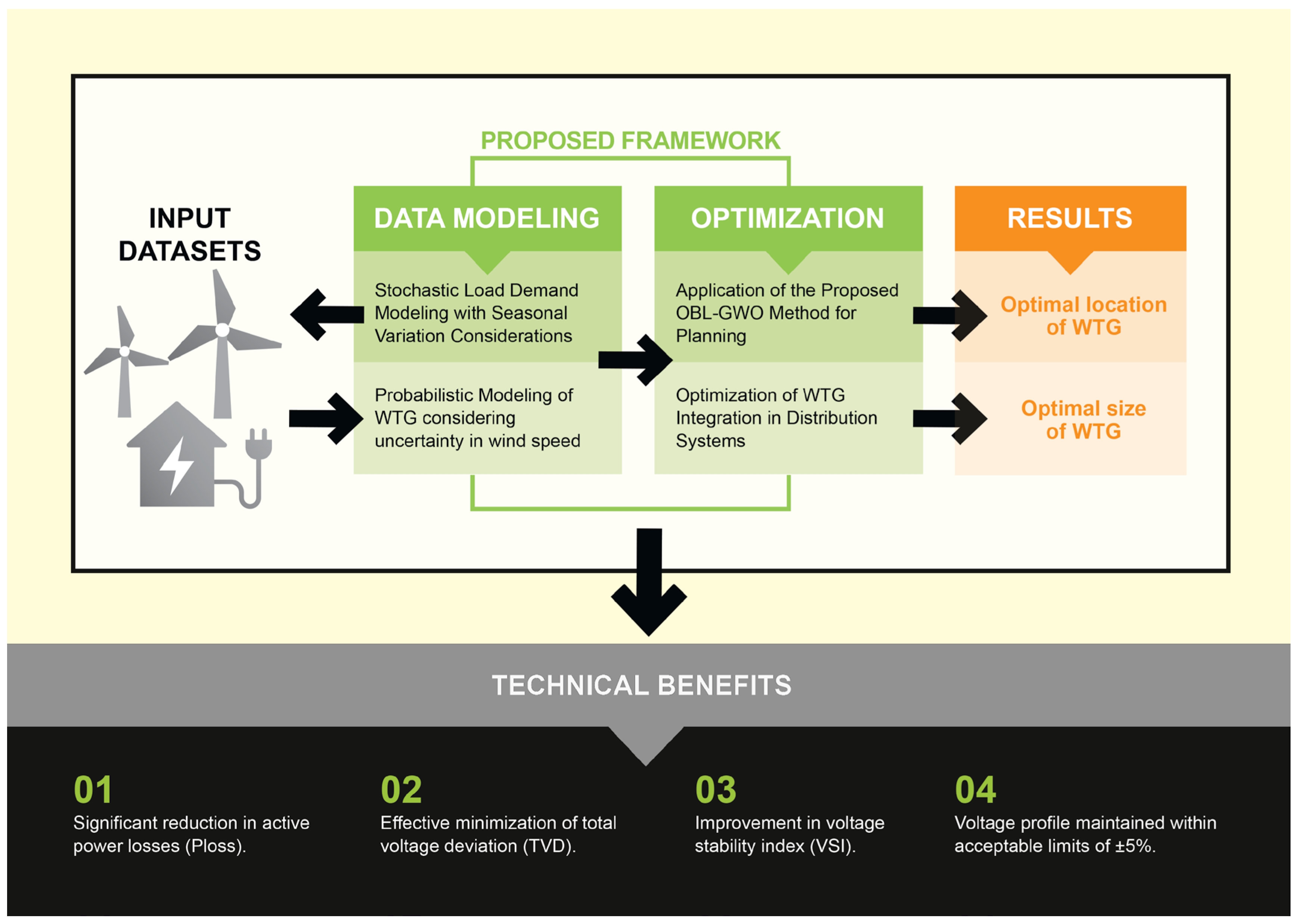
The above scrutiny of published work identifies gaps in previously reported research for tackling the distribution of DG sizes and locations in DNs. The metaheuristic techniques that predominate in most explorations of DG placement issues exhibit the deficiencies described for GWO. While OBL-GWO has proven effective in allocating PV-DGs, wind-based DGs involve distinct technical and stochastic characteristics. This study evaluates the adaptability and performance of OBL-GWO for optimal wind DG allocation under probabilistic and seasonal conditions. The proposed augmentation of GWO with OBL for wind turbine generation (WTG) positioning addressed the main research gap. While not ensuring a global optimum solution, the developed methodology generates outcomes superior to reported results obtained from recognized optimization methods. An additional notable gap was uncovered: lack of real-world weather or demand data included in prior modeling, which failed to encapsulate important dimensions related to seasonal variability, a factor that should be examined in analyzing the stochasticity and uncertainty associated with both generation and demand. The aim was to fill these gaps by optimizing multiple technical objectives: minimized power losses ( P l o s s ) and TVD, improved VSI, and voltage profiles kept within ±5% of allowable limits. Figure 1 outlines the primary stages of the developed framework and optimization methodology. Real-world operational variations often cause domain shifts that reduce the performance of data-driven diagnostic or optimization models, highlighting the need for adaptive techniques under uncertain conditions [40].
Unlike prior OBL-GWO variants that evaluate on deterministic benchmark functions or generic engineering tests, this work is the first to deploy OBL-GWO for WT siting/sizing in a radial ADN under seasonal stochasticity and multi-year growth. As summarized in Table 1, we build a 5-year Riyadh wind-and-load database, model seasonal wind via Weibull and stochastic load noise, incorporate demand growth (5.48%/yr over 20 years) into the planning baseline, and validate it on IEEE-33 with multi-objective technical metrics (Ploss, TVD, VSI, and V m i n ). Furthermore, the proposed approach has been benchmarked against the standard GWO as well as several widely recognized metaheuristic techniques reported in the literature. The combination of OBL-GWO using real seasonal data and considering load growth in the planning of ADN is, to our knowledge, absent from prior OBL-GWO literature.
The work presented in this paper offers several key contributions, including:
  • Execution of the OBL-GWO method for optimal allocation of WTG-based DGs in a radial distribution network, achieving up to 95.16% reduction in active power losses compared with the base case and 79.7–95.16% reduction compared with standard GWO across different scenarios.
  • Improvement in TVD by 96–99.7% and enhancement of the VSI by nearly 30%, with the minimum bus voltage raised from 0.907 p.u. (base case) to 0.994 p.u. under the proposed method.
  • Development and use of a five-year database of actual measurements of wind speed and load profile for Riyadh, Saudi Arabia to capture seasonal variability and stochasticity of both demand and generation for more realistic modeling.
  • Performance benchmarking and validation of the proposed methodology against benchmark techniques published in the literature using the IEEE 33-bus system across multiple WTG-DG penetration scenarios, confirming superior performance in terms of loss reduction and voltage profile improvement.

2. Modeling REG and Demand Uncertainty

Planning for and generating anticipated power can be markedly undermined by the stochastic nature and rapid variations in wind speed. This study explored probabilistic load modeling that mimics the unpredictability of generation vis-à-vis demand by factoring in random seasonal changeability, thereby improving the accuracy of planning strategies.

2.1. Wind Turbine Generation Modeling

Simulation criteria for determining appropriate WTG locations included notable seasonal fluctuations in wind patterns and significant differences between summer and winter wind speeds. Based on these criteria, Riyadh, Saudi Arabia, was chosen as the study location.

2.1.1. Wind Speed Modeling

Riyadh’s desert environment features enormous seasonal wind speed fluctuations, caused primarily by substantial seasonal differences in temperature and atmospheric pressure. Precise, strategic REG project planning calls for incorporation of these kinds of variations into wind energy modeling. Accurate and realistic WTG modeling that produces more realistic results that align with very low or very high speeds is therefore critical and requires consideration of the impact of seasonal wind speed changes on energy generation, economic viability, and system stability. One of the most effective and commonly used published methodologies for modeling these stochastic wind speeds is a Weibull function. Weibull modeling of wind speed data entails the following steps:
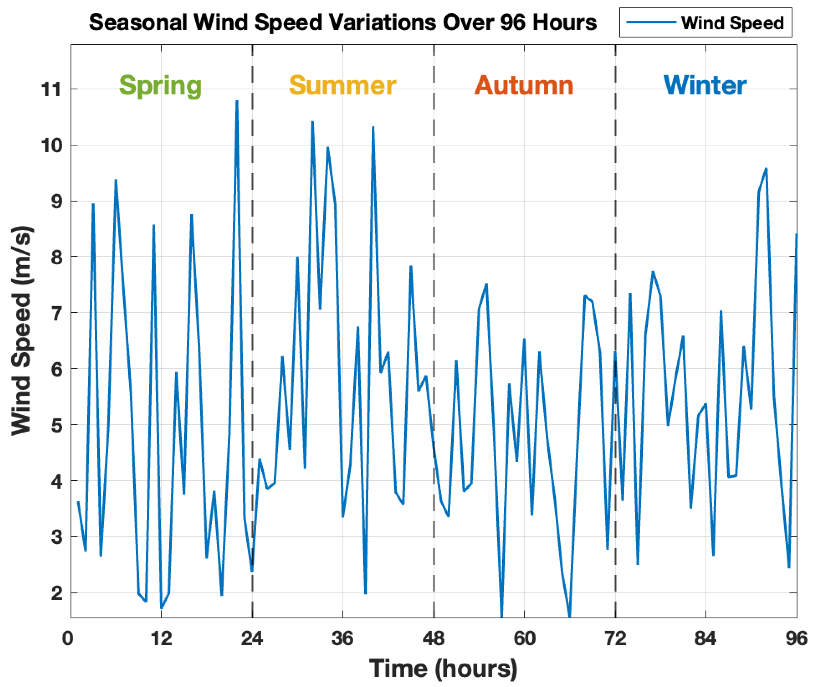
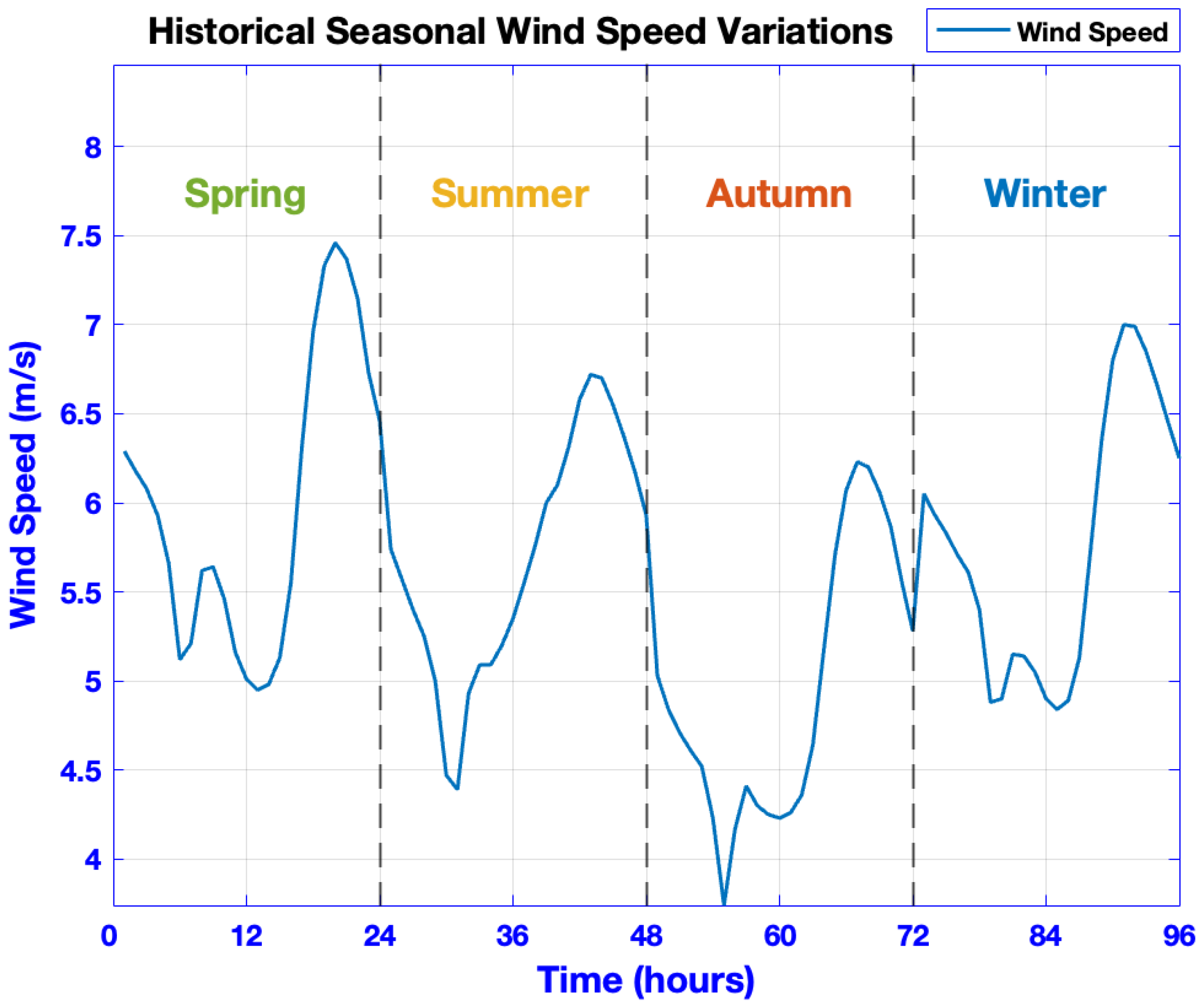
  • Step 1: To provide enhanced five years of historical wind speed data for Riyadh at 100 m height (the mean hub height of most wind turbines) were collected from [41]. The data were averaged so that each 24 h profile represents a typical day for a specific season, resulting in 96 hourly profiles across the four seasons. Figure 2 illustrates the five-year averaged seasonal variations in wind speed over 96 h.
  • Step 2: Use the five years of historical data to calculate hourly means for each season. Table 2 presents the results, which reveal seasonal variations in wind speed averages. For each season, compute hourly averaged mean and standard deviations and also record those values in the table for use in modeling the Weibull function parameters.
  • Step 3: Apply the seasonal mean and standard deviation values from Table 2, along with Equations (1) and (2), to estimate the Weibull function parameters k and c , respectively, for each season [42].
    k = σ v 1.086 ,
    c = v Γ 1 + 1 k ,
    where k is the distribution’s shape parameter, c is the distribution’s scale parameter, and Γ is the Gamma function that extends the factorial function to non-integer numbers.
    The Weibull function parameters k and c were defined for each season:
    For spring: k spring and c spring .
    For summer: k summer and c summer .
    For autumn: k autumn and c autumn .
    For winter: k winter and c winter .
  • Step 4: Using a Weibull PDF, apply the previously defined Weibull distribution parameters for generating random wind speed data for each season, with the parameters substituted into the Weibull PDF equation as given in Equation (3) [42]:
    f ( v ) = k c v c k 1 e v c k ,
    where v represents the input random wind speed variable ( v 0 ).
Table 2. Averaged wind speeds across four seasons.
HourSpringSummerAutumnWinter
0.006.295.745.036.05
1.006.185.574.845.93
2.006.085.404.715.83
3.005.935.254.615.71
4.005.665.004.525.61
5.005.124.474.235.40
6.005.214.393.744.88
7.005.624.934.174.90
8.005.645.094.415.15
9.005.465.094.305.14
10.005.165.204.255.05
11.005.015.354.234.90
12.004.955.554.264.84
13.004.985.764.364.89
14.005.136.004.645.13
15.005.556.105.185.73
16.006.326.315.716.35
17.006.966.586.076.80
18.007.336.726.237.00
19.007.466.706.206.99
20.007.376.556.066.85
21.007.156.375.876.66
22.006.736.175.566.45
23.006.465.935.286.25
Mean5.995.674.945.77
Std   dev   ( σ )2.522.412.122.28
Figure 3 displays the Weibull distribution functions that represent wind speed variations across four seasons. Observable fluctuations and sharp spikes in wind speed data reflect actual wind speed variations during a typical day. Spring and summer clearly exhibit the greatest wind speed peaks and variations due to their higher means and standard deviations: wind speeds reach between 10 m/s and 11 m/s. In contrast, the lower means and standard deviations of autumn and winter translate into slower wind speeds and less variation, with peak levels between 7 m/s and 8 m/s, except for occasional winter spikes.
The corresponding Weibull distribution parameters have been estimated to capture the statistical nature of wind variability. Table 3 shows the final shape and scale parameter ( k & c ) for each season, along with their 95% confidence intervals. These results show that the Weibull model provides a consistent and reliable fit across all seasons, with the parameter changes clearly reflecting seasonal shifts in wind behavior. Including the confidence intervals adds robustness to the modeling, ensuring that the estimated parameters account for uncertainty in the wind data and provide a solid foundation for the subsequent WTG allocation analysis.

2.1.2. WTG Modeling

In this study, the wind turbine is modeled using a standard piecewise linear power curve that represents the behavior of modern Doubly-Fed Induction Generators (DFIGs), it has been implemented using Equation (4) to model the WTG [43]. Specifically, the GE 1.5sle unit was adopted, with cut-in, rated, and cut-out wind speeds of 3 m/s, 12 m/s, and 25 m/s, respectively, and a rated power of 1.5 MW [44]. This turbine was chosen because its operating range aligns closely with the measured wind statistics in Riyadh, where most seasonal wind speeds fall within the 3–12 m/s band. This makes it suitable for reliable energy capture while remaining compatible with distribution system operational limits.
P w g ( v ) = 0   for   v < v w i & v > v w o P w r v v w i v w r v w i   for   v w i v v w r P w r   for   v w r < v v w o ,
where P w g ( v ) = output power, P w r = rated power, v w i = cut-in speed, v w o = cut-out speed, and v w r = rated speed.

2.2. Load Modeling

Since Riyadh’s climate features intense heat and since temperature alters electricity usage, power demand and load profiles are heavily impacted by seasonal shifts [45], including by extended or shortened daylight hours that can affect day-to-day load timing. To obtain a precise reflection of actual conditions, load modeling must therefore include consideration of seasonal changeability.

Computation of the Base Load

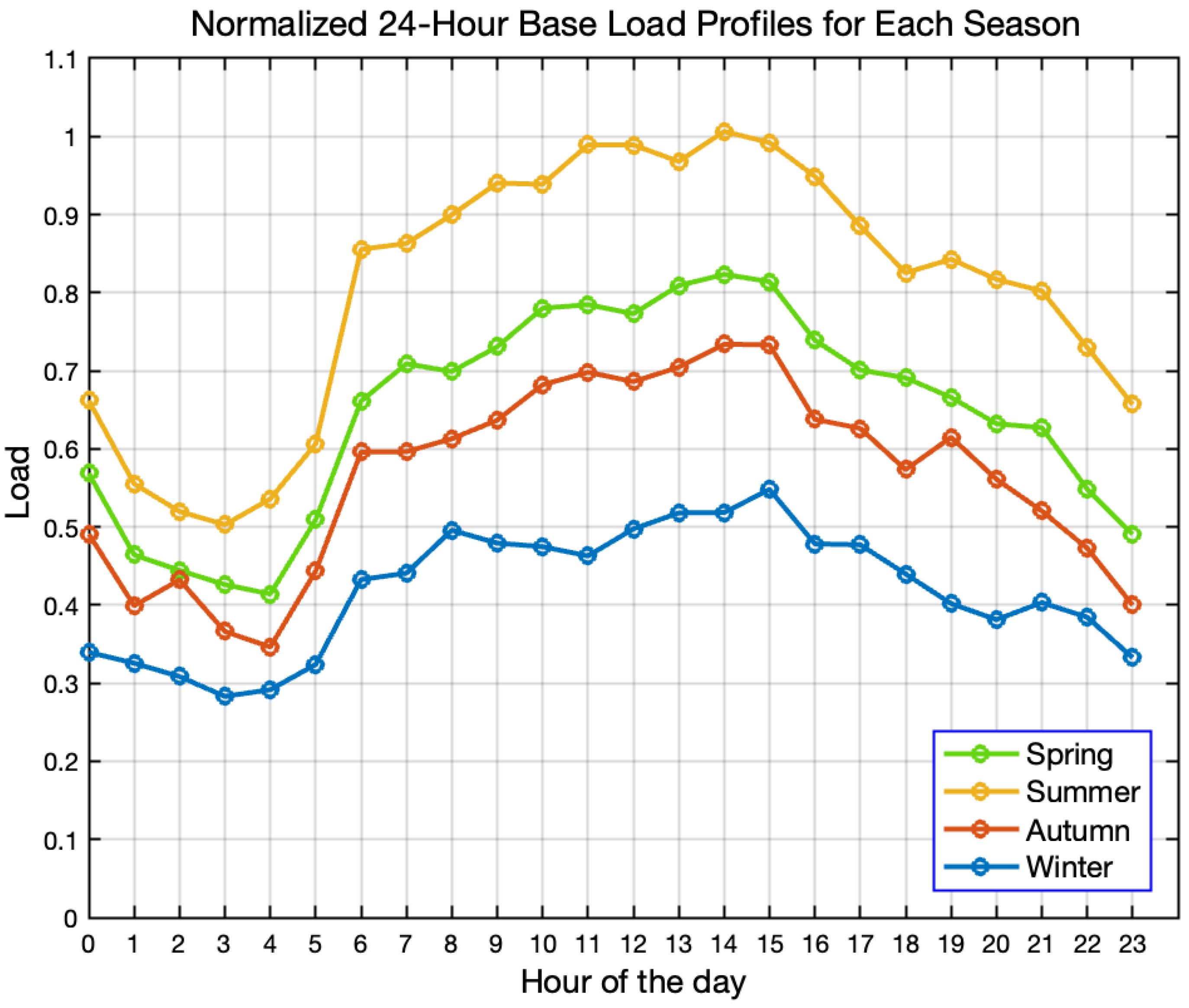
The most recent two years’ worth of hourly use statistics for Riyadh were obtained, analyzed, and cleaned. The hourly electricity consumption data for Riyadh were obtained in collaboration with the Saudi Electricity Company (SEC) and cannot be shared publicly due to confidentiality agreements. Appropriate corresponding time stamps were assigned, and the data were sorted: spring (March, April, May), summer (June, July, August), autumn (September, October, November), and winter (December, January, February). Employing Equation (5), seasonal hourly usage statistics were normalized to the absolute hourly peak load value. The resultant scaled seasonal usage was then mapped as shown in Figure 4.
N o r m a l i z e d   L o a d   P r o f i l e   ( t )   =   a v e r a g e   l o a d   p r o f i l e   ( t ) P e a k   L o a d ,
Conversion of these normalized base load profiles into real-life values that mirror the 24 h IEEE 33-bus test system demand was followed by the scaling of each profile to be in line with the peak load of the IEEE 33-bus system (3.715 MW).

2.3. Yearly Load Increases

Yearly load increases constitute a critical factor in power system design that has nonetheless been overlooked in most literature reports [46]. Any modeling that exclusively features fixed loads throughout the system life fails to accord with actual conditions. Prior design investigations such as [46] have been targeted at examining multi-year load expansion. Because electricity projects are expected to last longer than 20 years, taking yearly increases in demand into account is vital for guaranteeing long-term reliability and sufficiency. Historical Riyadh data had already been analyzed to reveal the approximate yearly demand growth: 5.48% [45]. For this study, the subsequent modeling phase was to apply the basic load growth equation to establish the growth factor for multiplication by the seasonal base load. This baseline is projected over a 20-year planning horizon using Equation (6).
T o t a l   g r o w t h   f a c t o r = ( 1 + a n n u a l   g r o w t h   r a t e ) years = ( 1 + 0.0548 ) 20 = 2.91 ,

2.4. Modeling Seasonal Patterns and Stochasticity

For spring, summer, autumn, and winter, we generated a noise with a normal (Gaussian) distribution. To replicate random changes in demand, the historical data were used for computing a discrete mean and standard deviation for each season’s noise. To discover how noise varies across seasons when seasonal elements are taken out, each hourly time stamp was compared against the average seasonal load profile, and the results were applied to compute the average hourly mean and standard deviation of each season’s noise, as expressed in Equation (7):
Noise t = H i s t o r i c a l   L o a d   ( t )   Seasonal   Average   Load   ( h ) ,
Simulation of the stochasticity of the seasonal data was achieved through two steps: deriving a Gaussian noise from the computed mean and standard deviation of the noise PDF, followed by producing a Gaussian noise with a normal distribution using Equation (8) [47]:
f n ( l ) = 1 σ n 2 π e x p ( l μ n ) 2 2 σ n 2 ,
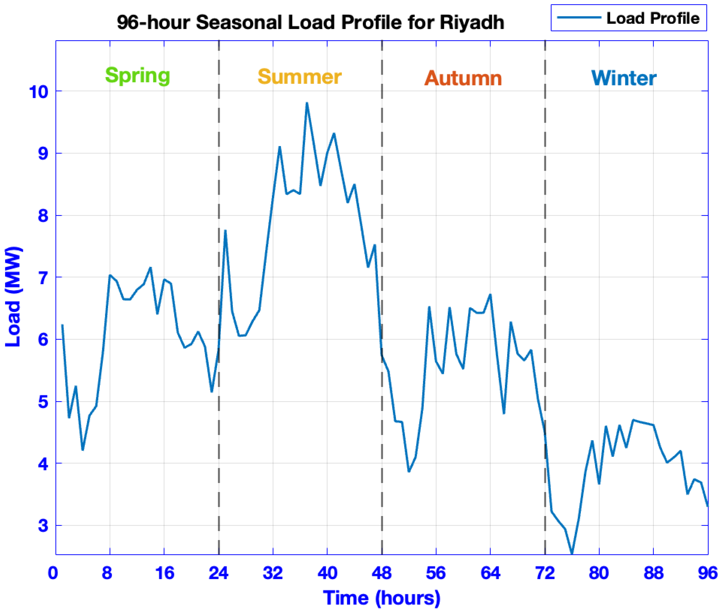
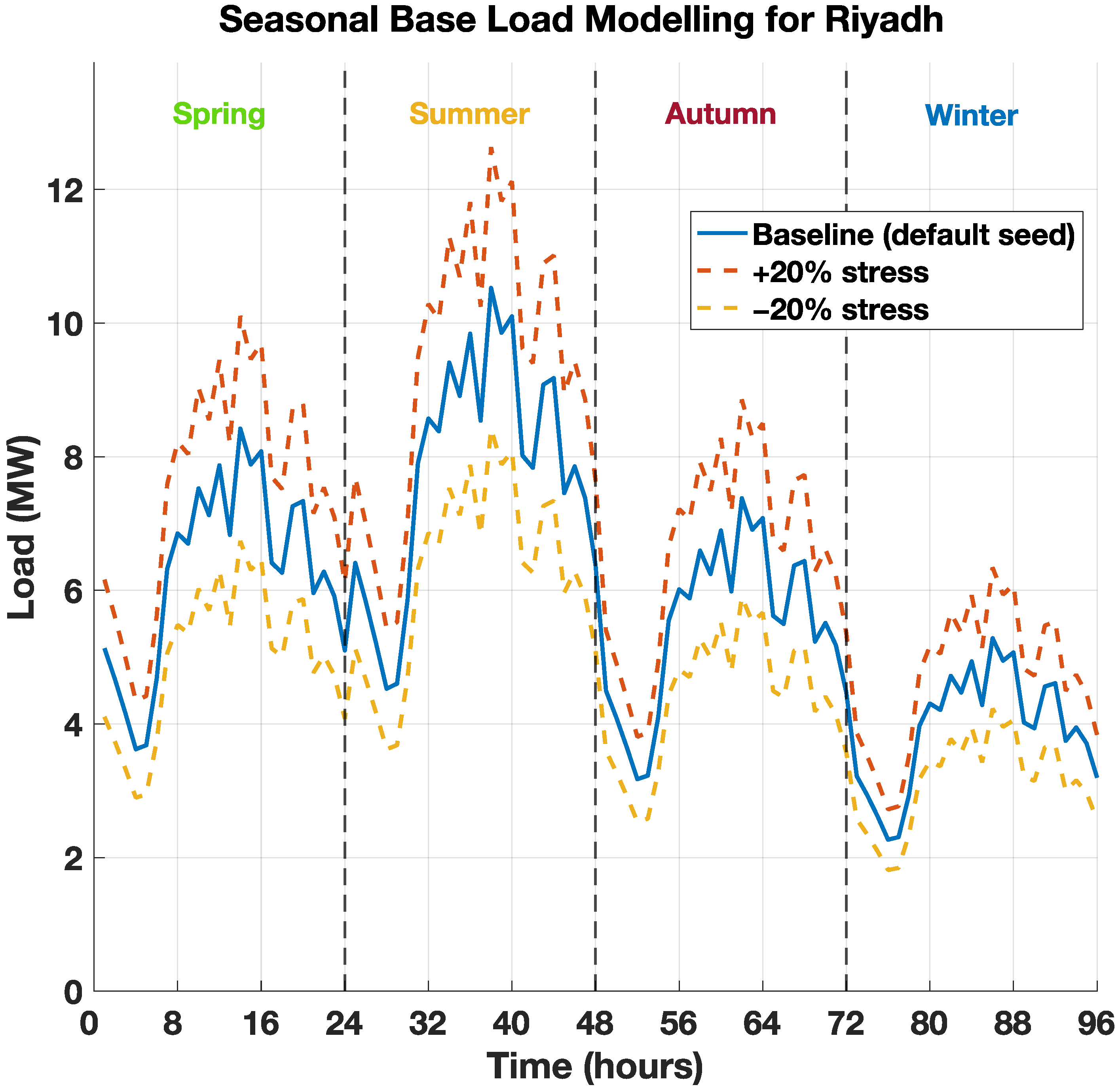
where f n ( l ) denotes the value of the noise PDF; l indicates the load, which stands for a random variable; μ n signifies the average noise distribution mean; σ n is the sum of the noise distribution standard deviations; and σ n 2 represents the distribution noise variance. As Figure 5 indicates, the modeling of the Riyadh seasonal profile was organized in the following order: spring covers the first 24 h and summer stands for the second 24 h (24th to 48th hours), followed by the third and fourth 24 h, which, respectively, denote autumn and winter.
The seasonal load baseline was obtained from normalized 24 h profiles of the IEEE-33 bus system, scaled by the system peak demand (3.715 MW) and projected over a 20-year horizon using a 5.48% annual growth rate. For clarity, the 96 h block was constructed sequentially: hours 1–24 represent Spring, hours 25–48 represent Summer, hours 49–72 represent Autumn, and hours 73–96 represent Winter. Gaussian noise with independent random seeds was applied to each 24 h segment. To represent short-term stochastic variability, zero-mean Gaussian noise was superimposed on the baseline profile, with the standard deviation set to 6% of the hourly load and values clipped at ±3σ to prevent unrealistic extremes; all loads were constrained to be non-negative. To confirm robustness, the seasonal profiles were regenerated under five independent random seeds (1, 11, 21, 31, 41). Across these runs, both peak demand and total energy showed very small variations (coefficients of variation < 2%), confirming stability with respect to random initialization. Stress tests were conducted by uniformly scaling the entire stochastic profile by ±20% to represent typical rare operating conditions which has been discussed further in stability analysis Section 7.5.
The seasonal load profile was implemented as a 96 h dataset, obtained by linking four representative 24 h blocks (Spring, Summer, Autumn, Winter). This inevitably introduces artificial discontinuities at the seasonal boundaries; however, these do not influence the results, since each hour is simulated as an independent steady-state operating point in the load-flow analysis. The purpose of 96 h linking is to captures seasonal variability while reducing framework complexity and computational cost, compared to simulating a full year of hourly data.

3. Problem Formulations

To improve system performance, effective DG positioning in an ADN necessitates analysis of multiple objectives: minimized power losses, viable voltage regulation, adherence to system restrictions, and attention to randomness. The following subsections discuss the problem formulation.

3.1. Objective Functions

The principal aim of the framework proposed for this research was to satisfy four primary technical objective functions, for which equations were implemented in MATLAB code, as detailed in this section: reduced P l o s s and Q l o s s , minimized TVD, and improved VSI.

3.1.1. Active Power Loss Reduction ( P L o s s )

Real power losses attributable to distribution losses and inferior system efficiency are indicated by the R P L measure computed according to Equation (9). The calculation of the objective function for minimizing reactive power loss is set out in Equation (10) [48]:
R P L = k = 1 N b r P L ( k , k + 1 ) ,
O F 1 = m i n   P L o s s ,
where k represents the bus number, and N b r denotes the total number of branches.

3.1.2. Reactive Power Loss Reduction ( Q L o s s )

In Equation (11), Q P L stands for the dissipated reactive power, and the objective function for minimizing reactive power loss is expressed in Equation (12) [48]:
Q P L = k = 1 N b r Q L k , k + 1 ,
O F 2 = m i n   Q L o s s ,

3.1.3. TVD Minimization

A measure of the amount by which each load bus deviates from the others, the TVD points to voltage level fluctuations and departures from the preferred norm, which can undermine performance [49]. Minimizing the TVD safeguards voltage supply quality. Equation (13) spells out the TVD calculations, and Equation (14) presents the objective function for TVD minimization [50]:
T V D = a = 1 n V a V r e f 2 ,
O F 3 = min   V D ,
where V a indicates the actual voltage, V r e f is set at 1.0 p.u., a denotes the bus number, and n specifies the number of buses.

3.1.4. VSI Enhancement

When bus voltages cannot be determined with surety, the results destabilize voltages and create havoc in DNs. As a pivotal indicator of stability, the VSI acts as a vital barometer of network security, and curbing VSI values for all buses can forestall instability. Determining the most effective DN positions for DG units promotes a healthy VSI, thus keeping appropriate voltage levels at each bus. For this study, Equation (15) was used for computing the VSI at each bus. A near-zero value means imminent collapse of a bus voltage. The goal is to optimize the minimum VSI by making sure that V S I k + 1 stays as close to 1 as possible, thereby improving voltage stability and total performance. Equation (16) sets out the objective function for maximizing the VSI for each branch k to (k + 1) [50]. In Equation (17), the VSI objective was reformulated as minimizing 1 / m i n   ( V S I ) . This is mathematically equivalent to maximizing the weakest bus VSI. Since the values of VSI remain strictly positive for all feasible power flow solutions, numerical instability near VSI → 0 does not occur. Moreover, collapse states with near-zero VSI are inherently prevented by the voltage magnitude and current constraints already embedded in the optimization, ensuring bounded and consistent evaluations across runs.
V S I k , k + 1 = V k 4 4 P k + 1 R k , k + 1 + Q k + 1 X k , k + 1 × V k 2 4 P k + 1 X k , k + 1 Q k + 1 R k , k + 1
O F 4 = max   min ( V S I k , k + 1 )   ,
O F 4 = min   1 min   ( V S I k , k + 1 )   ,

4. Multi-Objective Function Formulation

Optimizing the technical benefits of WTG placement in ADNs involved four technical parameters: P l o s s , Q l o s s , TVD, and the VSI. These factors are evaluated simultaneously, alongside compliance with relevant operational constraints, as outlined in the following subsection. The mathematical formulation of the multi-objective function (MOF) is defined in Equation (18) with each factor normalized using the Weighted Sum Method (WSM). Each parameter is divided by its base value for harmonious and viable optimization that enables technical factors to be compared at identical scales, with equal weights assigned, and with balanced compromises among objective functions. This process also keeps the algorithm from being dominated by objectives with higher absolute values.
O F T = w 1 O F 1 P L no DG + w 2 O F 2 Q L no DG + w 3 O F 3 T V D no DG + w 4 O F 4 V S I no DG ,
where O F T stands for the MOF, and w 1 , w 2 , w 3 , and w 4 are weighting coefficients for each optimization factor such that the sum of the absolute coefficient values equals 1. Most verification and standardization research has involved WSM in which the weighting coefficients are divided equally. The four weights were thus fixed at 0.25 each, to be later modified according to decision-maker or planner preferences. To verify robustness, we have tested additional weight samples, such as (0.40, 0.40, 0.10, 0.10) and (0.10, 0.10, 0.40, 0.40) to emphasize loss reduction and voltage stability, respectively. As shown in Table 4, varying the weights did not change the scenario ranking or optimal locations. It only shows marginal shifts in objective values, confirming robustness of the default equal weighting.
The set values P L no DG , Q L no DG , T V D no DG , and V S I no DG designate the system performance metrics of the IEEE 33-bus base case. O F 1 , O F 2 , O F 3 , and O F 4 respectively denote the objective functions for P l o s s ,   Q l o s s , TVD, and VSI, which are detailed below.
Results showed that only marginal shifts in optimal locations and sizes, with all cases preserving the same ranking of scenarios and significant improvements over the base case. This indicates that the chosen equal weighting does not bias the conclusions. It should be noted that weighted-sum formulations automatically turn multiple objectives into a single scalar value. This can make it difficult to see the whole Pareto front and miss out on trade-off solutions. However, in this study the objectives were found to be largely aligned, making the equal-weight WSM formulation adequate for practical ADN planning.

4.1. System Constraints

For the best DN operation and planning, several constraints must be in force to guarantee that the system provides reliability and stability within physical and operational limits. These restrictions are essential for specifying the feasible solution space for optimization problems, especially for DG positioning and sizing. The main system constraints examined in this study are detailed below: power balance, voltage, current, DG capacity, DG location, and DG power factor. The methodology for confirming the system’s operational viability through power flow calculations is also described.

4.1.1. Power Balance Constraint

Power flow analysis requires that a mandatory equality constraint termed power balance be fulfilled as a means of ascertaining that demand power plus power losses equate to total generation. This balance must be satisfied for both active and reactive power elements, as detailed in Equation (19) and Equation (20), respectively, [51]:
P G + k = 1 N D G P D G , k = i = 1 N B   P D e m a n d ,   i b = 1 N B R   P L o s s ,   i   ;       k = 1 N D G ,
Q G + k = 1 N D G Q D G , k = i = 1 N B   Q D e m a n d ,   i b = 1 N B R   Q L o s s ,   i ;       k = 1 N D G ,
where k denotes the number of DGs; i and b represent bus and branch numbers; Q G and P G indicate the respective reactive and active power injected by the main substation; and Q D G , k and P D G , k stand for the reactive and active power, respectively, produced by the k t h DG.

4.1.2. Voltage Constraints

The purpose of voltage constraints is to verify that voltage magnitude V i at any bus i is within ± 5 % of the RDN rated voltage. As set out in Equation (21), in per unit calculations, this figure falls between a V m i n value of 0.95 p.u. and a V m a x value of 1.05 p.u.; Voltage deviations outside 0.95–1.05 p.u. are penalized using a quadratic penalty function. A soft violation within 0.90–0.95 or 1.05–1.10 p.u. incurs a moderate penalty (102), while violations beyond 0.90–1.10 p.u. incur a large penalty (104), effectively restoring feasibility.
V m i n V i , i + 1 V m a x ,

4.1.3. Branch Current Constraints

Line overloads were penalized proportionally to the overload percentage. Exceeding the thermal limit by 1% incurred a linear penalty scaled by 103, which grows with the severity of the violation. To fulfill current or thermal limits, the branch current I i , j   between nodes i and j cannot be greater than that branch’s maximum capacity   I i , j m a x , as stipulated in Equation (22):
I i , j       I i , j m a x ,

4.1.4. DG Capacity Constraints

Starting DG capacity is specified according to explicit minimum and maximum active and reactive power output capacities, respectively, as detailed in Equations (23) and (24) [38]. The minimum–maximum generation bounds for each DG were defined such that the total installed DG capacity does not exceed 100% of the IEEE 33-bus system base capacity, corresponding to an upper limit of 3.715 MVA. Solutions proposing DG capacities outside the specified min–max bounds were discarded by assigning a fixed penalty (105), ensuring only feasible DG sizes remained. The achieved total DG capacities per scenario are reported in the results tables and show that the optimal solutions did not reach this upper bound. This ensures penetration remains realistic without artificially limiting the feasible search space.
P D G , i m i n P D G , i P D G , i m a x ,
Q D G , i m i n   Q D G , i Q D G , i m a x ,

4.1.5. DG Location Constraints

The limit expressed in Equation (25) prevents a DG unit from being installed at the slack bus (bus #1) since it serves as the slack bus. Equation (26) allows no more than a single DG to be placed at any individual bus, all while still adhering to the restriction on the maximum number of buses:
2 L D G i ,
L D G i L D G j N b u s ,
where L D G i and L D G j indicate the position of the i th and j th DG, N b u s is the number of buses.

4.1.6. DG Power Factor Constraints

When the optimal DG power factor must be established, to make certain that DG units are operating productively, the power factor is restricted to an upper limit of 1 and a lower limit of 0.9, as defined in Equation (27). Further, we have assumed that DGs are constrained to operate within 0.9 ≤ PF ≤ 1.0, indicating unity to lagging operation. This assumption ensures that DGs are primarily expected to inject active power while providing limited reactive power support (Q > 0). Leading PF operation (absorbing reactive power) was not included. The PF was assumed to be fixed during optimization rather than dynamically scheduled on an hourly basis. Moreover, power factor violations below 0.9 were penalized linearly with a weight of 103, ensuring that the optimizer always converged to feasible PF values within the 0.9–1.0 range.
0.9   Power   Factor   1 ,
To enforce these operational limits during optimization, a penalty-based constraint handling mechanism was adopted. For any candidate solution, violations of voltage, branch current, DG capacity, DG location, or DG power factor constraints were translated into additive penalty terms. Equation (28) represents the overall penalized objective function:
O F p e n = O F T + α v   ( Δ V ) 2 + α I   ( Δ I ) 2 + α P F   ( Δ P F ) 2 + α l o c N v i o l
where O F T is our main multi-objective function, ΔV, ΔI, and ΔPF denote the respective violations, N v i o l   is the number of location violations, and α values ( 10 2 10 6 ) are empirically tuned penalty coefficients (with α = 102 for voltage, α = 103 for current, and α = 105 for DG penetration in the reported runs). This formulation used to ensure that infeasible solutions are assigned sufficiently large penalties to restore feasibility while preserving search efficiency.
5. Power Flow Computation

Contrary to a transmission system, a RDN normally features a substantial reactance/resistance (R/X) ratio and unbalanced loads, so that conventional power flow techniques, e.g., the Gauss-Seidel method and Newton Raphson method (NRM), take an extremely long time or cannot converge. For this reason, with RDNs, numerous researchers opt for power flow analysis (PFA) approaches derived from Kirchhoff’s laws, e.g., the backward/forward sweep (BFS) power flow algorithm introduced in [6], the common choice for RDNs. Results of other work [52,53] demonstrated the utility of forward/backward sweeps in RDNs, but iterative approximations prove more suitable in meshed networks. Which PFA type is preferable is reliant on the design of the RDN. The iterative BFS method proceeds to the point of the bus voltage converging to a stable solution so that bus voltage shifts between repeated attempts drop below a stipulated tolerance. Initial bus voltages are first matched to that of the reference bus (typically 1 p.u.), and the starting branch currents are set to zero. Every iteration comprises two primary phases: a backward sweep and a forward sweep. The backward version entails recomputing branch currents from the end buses (leaves) in the direction of the root bus (source) according to the power mismatch: the difference between injected and load power. On the other hand, a forward sweep means that voltages are updated at each bus, from the slack bus through to the end buses. The fall in voltage over each branch is then computed based on branch currents and impedance. Figure 6 depicts an RDN scheme, with active and reactive power flows identified and with k denoting the bus number at the iteration under scrutiny.

5.1. Test System

The commonly used IEEE 33-bus test configuration was chosen for assessment purposes. All per-unit quantities in this study are referenced to a base of 3.715 MVA and 12.66 kV, consistent with the IEEE 33-bus system. Because it features in most reported work, evaluating the efficacy of new methodologies is more straightforward since fresh research results can be verified against those from prior studies. Figure 7 provides a circuit drawing of the IEEE 33-bus radial test topology.

5.2. Mathematical Formulation

Figure 8 is a line drawing of the DN radial topology. Equations (29) and (30), respectively, specify the formulation of the active ( P k ) and reactive ( Q k ) p o w e r .
P k = P k + 1 + P L D , k + 1 + R k , k + 1 ( P k + 1 2 + Q k + 1 2 | V k + 1 | 2 ) ,
Q k = Q k + 1 + Q L D , k + 1 + X k , k + 1 P k + 1 2 + Q k + 1 2 | V k + 1 | 2 ,
where k denotes the sending bus number, and k + 1 identifies the receiving bus number. P k and Q k   were computed in the backward direction-based Equation (31), and the receiving bus voltage ( V k + 1 ), in the forward direction from the square root of Equation (31).
V k + 1   2 = V k 2 2 R k , k + 1 P k + X k , k + 1 Q k     + R k , k + 1 2 + X k , k + 1 2 P k 2 + Q k 2 | V k | 2 ,
Equations (32) and (33) were applied for calculating the real ( R P L ) and reactive ( Q P L ) power losses, respectively, between the sending bus k and the receiving bus k + 1 [48]:
R P L k , k + 1 = R k , k + 1 P k 2 +   Q k 2 | V k | 2 ,
Q P L k , k + 1 = X k , k + 1 P k 2 + Q k 2 | V k | 2 ,

6. Optimization Methodology

The following subsections describe the approach applied for creating the new framework.

6.1. Overview of Grey Wolf Optimizer (GWO)

In the model presented here, GWO was executed for determining the best DG positioning. Unimodal and multimodal benchmark functions are usually employed for investigations of the exploration and exploitation efficacy of an optimization algorithm. Unimodal functions are suitable for exploitation benchmarking due to their single global optimum [17], but for assessing exploration, multimodal functions are preferable: multiplying at an enormously fast rate based on dimension, their numerous local optima enable them to evaluate an algorithm’s capacity for competently scrutinizing the search space while evading local optima. The GWO mathematical modeling required two phases involving separate core equations for each: encircling the prey and subsequently hunting and attacking the prey.

6.1.1. Encircling the Prey

Algorithm exploration, which in GWO is called encircling the prey, means computing how far apart the wolves and prey are. Equations (34) and (35) governed the modeling of this stage [17]:
X ( t + 1 ) = X p ( t ) A D ,
D = C X p ( t ) X ( t ) ,
where X ( t ) and X ( t + 1 ) give the locations of a gray wolf at iterations t and t + 1 , respectively, and X p ( t ) designates the position vector of the prey at iteration t . Vectors A and C , computed from Equations (36) and (37), respectively, dictate wolf moves and are vital for seeking good solutions in the search space. Vector C can be viewed as stemming from natural hindrances that prevent wolves from quickly and easily approaching the prey. The values of a and A are adjusted to even out exploration and exploitation. When |A| > 1, gray wolves must separate from the prey to discover superior solutions, but the reverse is true for |A| < 1: wolves have to move together in the direction of (i.e., attack) the prey [17].
A = 2 a r 1 a ,
C = 2 r 2 ,
where r 1 and r 2 represent random vectors within the range [0, 1], and a is a factor that decreases linearly from 2 to 0 over the course of the iterations, according to Equation (38).
a = 2 1 t / T ,
where t signifies the current iteration, and T stands for the maximum number of iterations.

6.1.2. Hunting and Attacking the Prey

A pivotal feature of GWO is the hunting mechanism, or exploitation. Alpha wolves α can recognize and pinpoint prey, which makes them capable directors of search space movements. Next best in executing this job are beta ( β ) and delta ( δ ) wolves. Each time the top three solutions are determined at any time in the search, the wolves must alter their locations according to preferable positions, as established by their closeness to the prey. Equations (39) and (40) are the mathematical equations that control this procedure [17]:
X 1 = X α A 1 D α , X 2 = X β A 2 D β , X 3 = X δ A 3 D δ ,
D α = C 1 X α X , D β = C 2 X β X , D δ = C 3 X δ X ,
The last of these tasks is to use Equation (41) to average the three best wolf positions in order to establish a revised gray wolf location [17]:
X t + 1 = X 1 + X 2 + X 3 3 ,
where X 1 = X α indicates the position of the alpha wolf (the best solution yet discovered), X 2 = X β signifies the position of the beta wolf (second-best solution), and X 3 = X δ represents the position of the delta wolf (third-best solution).
Based on Equations (39) and (40), the gray wolves (search agents) continue to revise their locations at each iteration until they have determined the optimal position yet discovered. Hunting ends with the wolves attacking the prey (converging to the optimal location).

6.1.3. Proposed GWO with OBL Augmentation (OBL-GWO)

Since GWO is susceptible to stagnation in local optima, it was augmented with OBL due to prior success with OBL in this context: it facilitates diverseness; helps the algorithm break free of local optima; and enhances learning, searching, and optimizing.
OBL features two primary techniques for establishing an opposite solution; which one is selected is reliant on the spatial extent of the search area for the particular problem [35]:
  • Opposite number method: This version of OBL involves an examination of the opposite of a real number x within the range [ a , b ] , where a and b are the lower and upper bounds of the solution space in the set of R. The inverse of the number x where x [ a , b ] is designated x ¯ and is computed according to Equation (42):
    x ¯ = a + b x ,
    The opposite number x ¯ is replaced by its matching solution x based on the fitness function. If x ¯ dominates x , then x = x ¯ .
  • Opposite point method: This method extends the opposition concept to encompass multidimensional points. X can be expressed as the vector X = x 1 , x 1 , , x n , where each x j is situated within its particular bounds a j , b j , and its correlated opposite point is designated X ¯ = x ¯ 1 , x ¯ 2 , , x ¯ n , to be computed as in Equation (43):
    x ¯ j = a j + b j x j ,
    where   j = 1 ,   2 ,   ,   n .
With this method, the opposite vector X ¯ is swapped for its matching solution X based on the fitness function. If X ¯ dominates X , then X = X ¯ .
In this study, the standard Grey Wolf Optimizer (GWO) has been enhanced by integrating the opposite point mechanism of Opposition-Based Learning (OBL), as formulated in Equation (43). This enhancement is particularly suitable for addressing the high-dimensional nature of the optimization problem, which involves a diverse set of decision variables, including discrete variables (bus locations) and continuous variables (active and reactive power ratings of distributed generators). Furthermore, the problem is governed by multiple operational constraints and objective functions. Consequently, each search agent or wolf in the algorithm represents a multi-dimensional solution vector rather than a single scalar value, with each dimension corresponding to a specific decision variable.

7. Results and Discussion

For the work presented here, conventional GWO was applied but with the inclusion of the new OBL-GWO algorithm for finding ideal WTG-type DG locations in RDNs. In this study, the new approach was assessed with respect to WTG integration only. Four placement scenarios were examined for both standard GWO alone and the new OBL-GWO variant:
  • Base Case: Normal network operation with no DGs;
  • Scenario 1: One WTG unit with an optimal power factor (OPF);
  • Scenario 2: Two WTG units with an OPF;
  • Scenario 3: Three WTG units with an OPF.
An OPF is assumed in all cases so that study findings can be compared to published outcomes since most related reports suggest the use of an OPF in WTG modeling.

7.1. Assessment of the Base Case

Implementing a base case, in which the IEEE 33-bus test system was analyzed and simulated alone with no DGs, facilitated comparison with other DG penetration configurations. Table 5 lists the test system specifications: total number of buses ( N b u s ) and branches ( N b r ) , nominal voltage, base power, and total system load (MVA).
MATLAB base case simulations involving no added DG units generated the base performance output shown in Table 6. Total active and reactive power losses were 210.07 kW and 142.43 kVAr, respectively, and the TVD came to 0.1328. The simulation results align with reported findings, with close to a ± 5 % error margin [51,54,55].
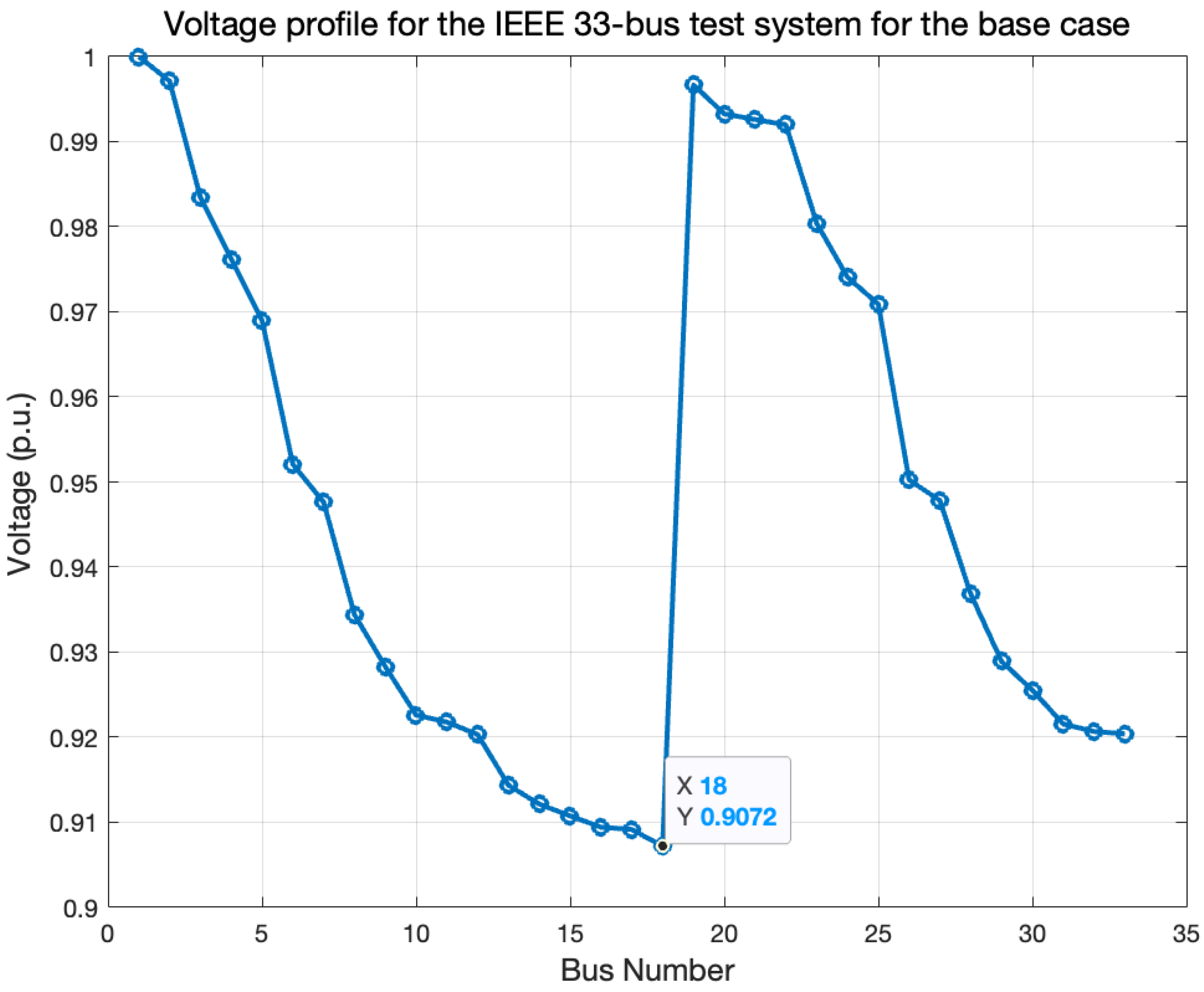
The power flow findings illustrated in Figure 9 reveal the voltage measurements across buses. Clearly visible in the voltage profile is a marked voltage drop located away from the substation along the RDN, especially at buses 18 and 33, where the voltage falls to minimum levels, with the lowest value of 0.9072 p.u. at bus 18.

7.2. Multi-Objective Optimization

Further testing involved implementing identical predefined configurations but with varied amounts of WTG integration, first with standard GWO and then with the developed OBL-GWO technique. For each approach, the results of the four scenarios were compared with respect to ideal locations, optimal DG sizing, P l o s s , and TVD and VSI findings. Standard GWO simulation was performed using MATLAB R2022a on a MacBook equipped with an Apple M1 Pro processor and 16.0 GB of RAM, running macOS Sonoma (version 14.5). The OBL-GWO simulation features the same predefined, different WTG integration scenarios, modeling input datasets and algorithm criteria as for standard GWO. Table 7 shows the specifications for both the GWO and OBL-GWO simulations.
The final reported runs correspond to random seeds {1, 11, 21, 31, 41}, with a stopping criterion of 200 iterations. Subject to the same predefined specifications, simulations using both conventional GWO and OBL-GWO generated the detailed results listed in Table 8.
Examining base case results against those for other scenarios (Table 8) makes it very clear that incorporating DGs can substantially decrease power losses and enhance the voltage profile. Detailed GWO and OBL-GWO findings are discussed in the next subsections. To ensure statistical rigor, for both GWO and OBL-GWO methods, 30 independent runs have been executed. Results show mean ± std, best, and worst values for Ploss, TVD, V m i n , and VSI. These are now presented in Table 9, and the findings confirm that OBL-GWO consistently delivers superior and more stable performance.

7.2.1. Conventional GWO Results

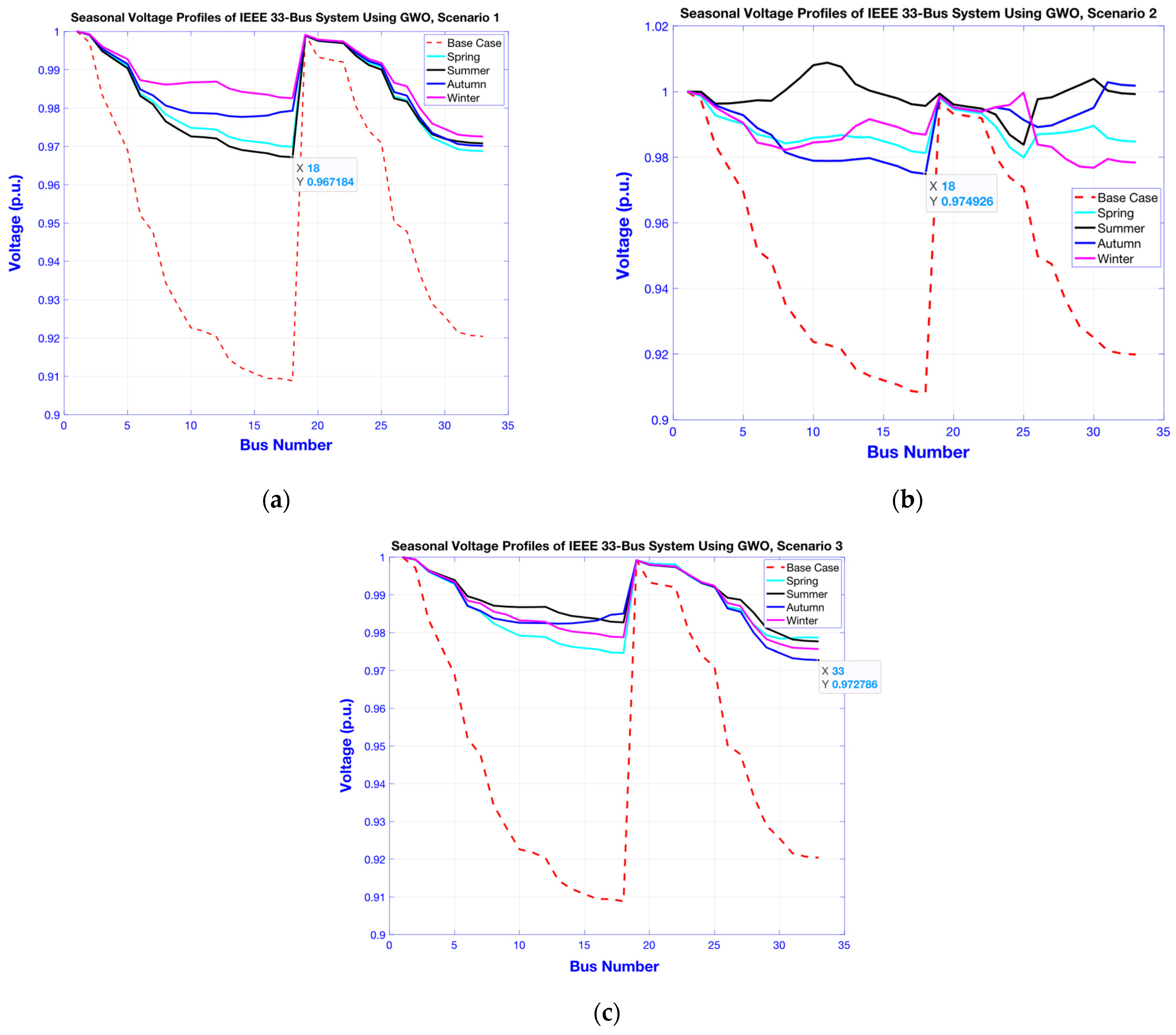
For the Scenario 1 simulation that entailed the use of standard GWO with 71.3% WTG integration, power losses decreased by 72.15%, the TVD was enhanced by 93.52%, and the VSI rose by close to 7% compared to the base case. With Scenario 2, despite the DG penetration being 9% lower compared to Scenario 1, the added WTG units that were optimally positioned in two ideally sized buses made the TVD substantially better by 98.72% and reduced the real power loss by 81.56% relative to the base case. With Scenario 3’s three WTG units incorporated at the best placements (bus 31, bus 25, and bus 32) and sizable WTG integration of about 81.16% of system capacity, further appreciable improvements vis-s-vis the base case was apparent with respect to real power loss (91.17%) and TVD (99.56%). Scenario findings were then mapped by season. Figure 10a–c display seasonal bus voltage profiles for GWO scenarios 1, 2, and 3, respectively, with the divergent base case graphing lines shown in each case. Vertical axes indicate per unit voltage quantities and horizontal axes note bus numbers. Due to the reduced wind speeds during the summer and autumn seasons, the minimum voltage was observed during these seasons at bus 18 for Scenarios 1 and 2, and at bus 33 for Scenario 3, with values of 0.967 p.u., 0.974 p.u., and 0.9727 p.u., respectively. This level is under the soft voltage limit of 0.95 p.u. (−5%) while still fulfilling the hard constraint of 0.9 p.u. (−10%) as the minimum permissible voltage.

7.2.2. Outcomes with OBL-GWO

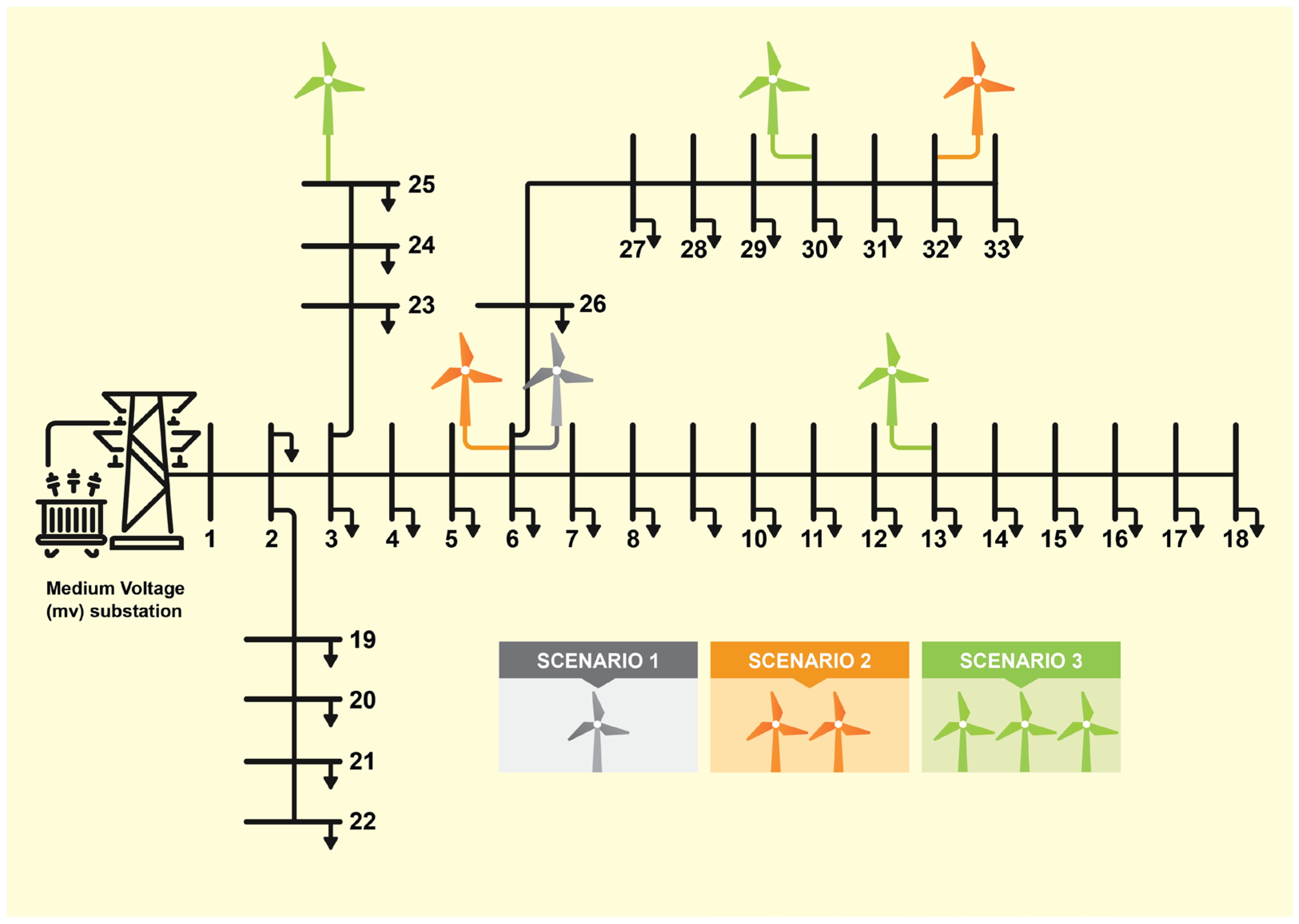
Figure 11 displays the IEEE 33-bus RDN scheme, with DGs embedded according to three predefined scenarios established according to the OBL-GWO technique. The designated network starting point is the medium-voltage (MV) substation. To highlight which buses were allocated DGs, the scenarios were given contrasting colors, with DG positions marked by color-coded wind turbine images. To enhance grid performance and achieve the study goals, the scenarios were chosen to improve network performance and accomplish the research objectives.
Table 7 shows that, for every DG penetration level, the new OBL-GWO technique unquestionably outperformed the base case in terms of power losses and voltage profiles. Scenario 1’s 68.9% WTG penetration reduced power losses by 79.7%, markedly enhanced TVD (by 96.39%), and raised the VSI by nearly 29.5%. The 16% step up in WTG integration under Scenario 2, featuring WTG units optimally located at two separate buses, resulted in a 98.27% healthier TVD and a 89.29% decrease in power losses. Scenario 3, with close to 92% WTG penetration from installations at buses 30, 13, and 25, produced an 95.16% decrease in power losses and a 99.7% improved voltage profile relative to the base case.
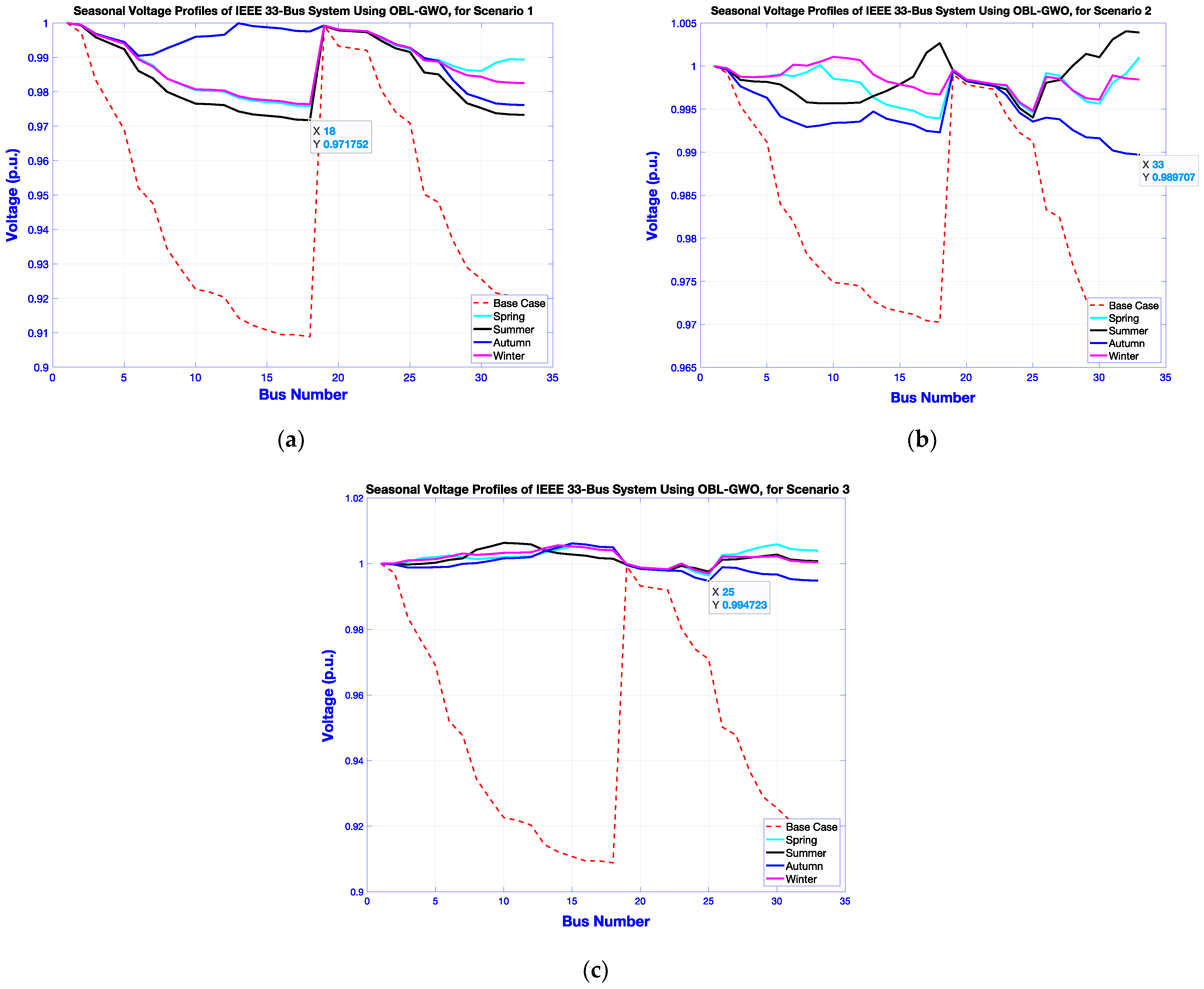
The OBL-GWO findings from the three scenarios were summarized as the seasonal voltage profile graphs displayed in Figure 12a–c. Profiles for every bus are included for each scenario and each season. Vertical axes designate voltage measurements (p.u.) and horizontal axes give the bus numbers. The OBL-GWO results revealed seasonal variations, with the lowest voltages recorded at bus 18, bus 33, and bus 25 at approximately 0.971 p.u., 0.989 p.u., and 0.994 p.u. for Scenarios 1, 2, and 3, respectively. These voltage drops are attributed to the reduced wind speeds during the summer and autumn seasons across all scenarios. However, levels were still within ±5% of permitted thresholds and were considerably better than test system operating parameters under the base case. In fact, the optimal voltage profiles for every scenario were those for spring, which are characterized by normal loads and moderate wind speed.
Overall, due to local load compensation resulting from DG integration, increasing the level of WTG penetration clearly leads to corresponding improvements in power loss P l o s s and voltage profile, particularly at lower penetration levels.

7.2.3. Comparative Evaluation of Standard GWO and Proposed OBL-GWO

To provide a complete overview, Table 10 summarizes the final performance metrics (Ploss, TVD, VSI, and V m i n ) for the no-DG baseline and Scenarios 1–3 under both GWO and OBL-GWO. The table shows the further improvements of both methods relative to the base case. It also shows the additional improvements achieved by OBL-GWO in comparison with the standard GWO. The results highlight that OBL-GWO consistently achieves greater reductions in losses and voltage deviations, while further enhancing VSI compared to both the baseline and standard GWO across all scenarios.
Before optimization, the base case exhibited a minimum bus voltage of 0.907 p.u. (at bus 18) and occasional branch overloads beyond rated limits. After optimization, in all OBL-GWO and GWO scenarios, the final converged solutions were strictly feasible where all bus voltages remained within 0.95–1.05 p.u. and no line overloads were observed. Therefore, the penalty terms were inactive in the final solutions, confirming that the reported results correspond to strictly feasible operating points.

7.3. Convergence Behavior

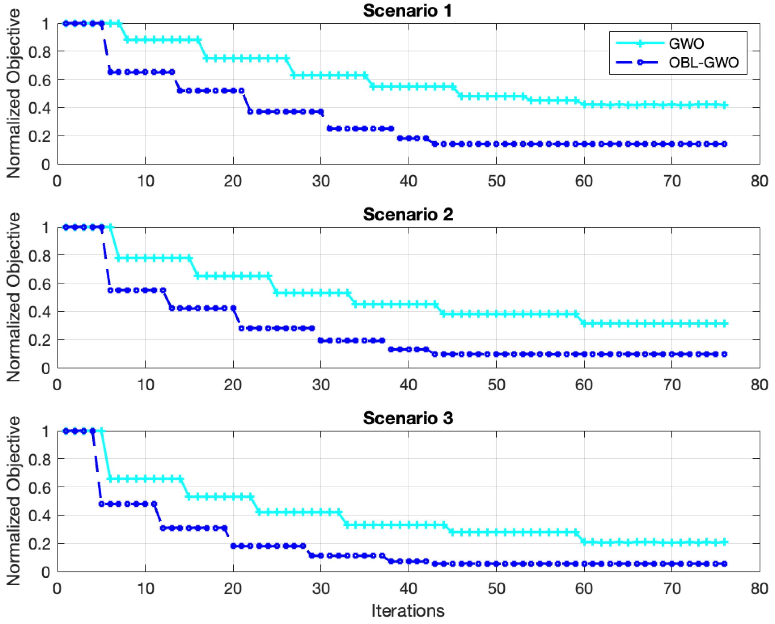
To compare the performance of the standard GWO and the proposed OBL-GWO algorithm further, Figure 13 presents the convergence curves across all scenarios that clearly demonstrate the superior performance of the OBL-GWO method. In each scenario, OBL-GWO converges faster and reaches a lower normalized objective value compared to the standard GWO. In Scenario 1, OBL-GWO converges to a value near 0.14, whereas the GWO settles around 0.42. In Scenario 2, OBL-GWO again outperforms at approximately 0.1, compared to GWO’s lowest value of about 0.31. Moreover, the performance further improves in Scenario 3, where the OBL-GWO achieves a normalized objective value of approximately 0.05, and GWO levels off at 0.2. The improvement is particularly evident during the early iterations. OBL-GWO rapidly approaches optimal solutions, while GWO converges more slowly and often settles at higher objective values. The performance gap between the two methods becomes significant as the number of WTGs increases. This indicates that OBL-GWO handles increased problem complexity more effectively. Additionally, the stability of the OBL-GWO results in the flat convergence curves after early iterations, suggesting that the algorithm avoids premature convergence and maintains robustness throughout the optimization process.
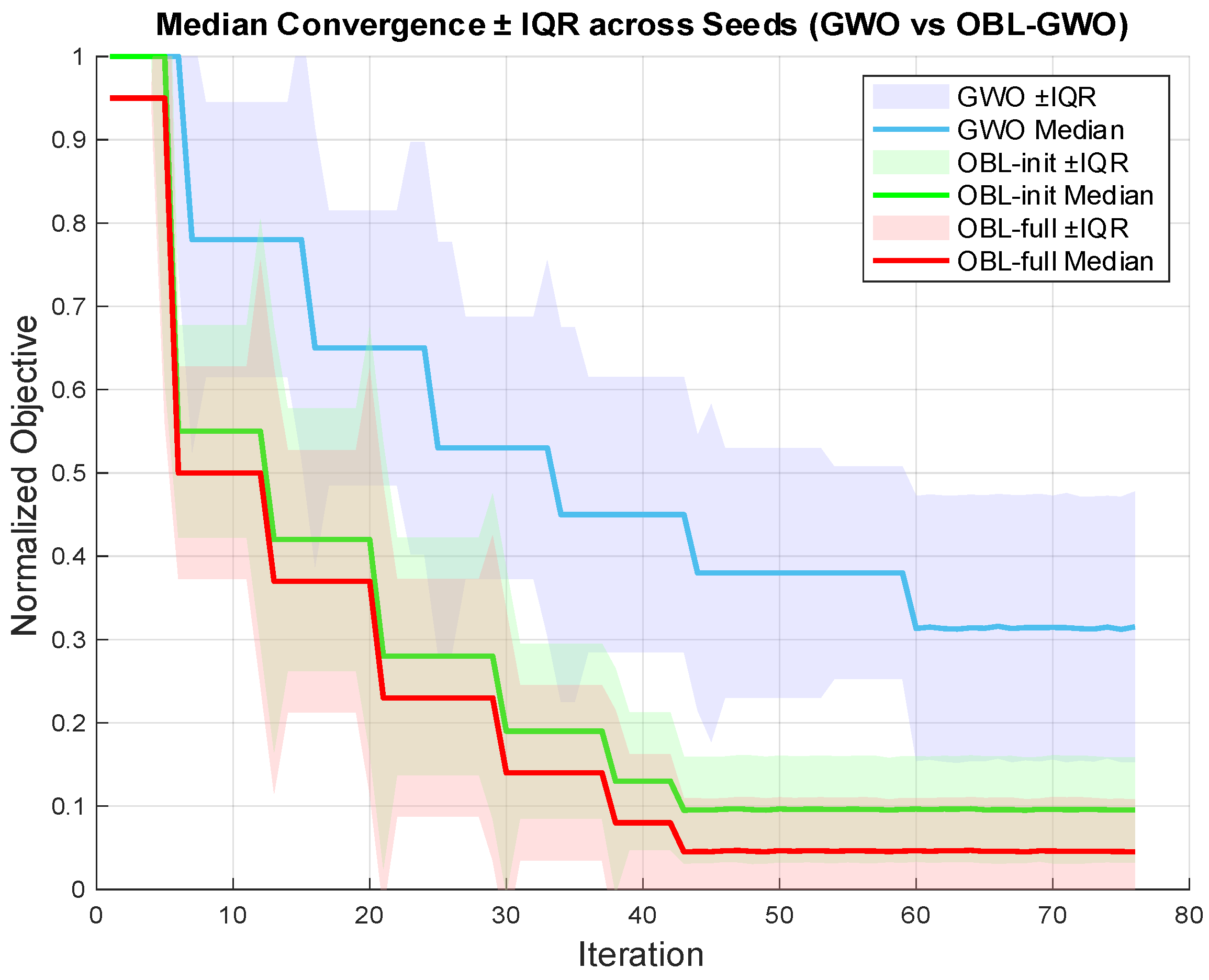
To strengthen the convergence analysis, both GWO and OBL-GWO were executed for 30 independent runs for scenario 2, and median convergence curves with interquartile ranges (IQR) were plotted with shaded interquartile (25th–75th percentile) bands (Figure 14). The results confirm that OBL-GWO converges more rapidly and with lower variance compared to GWO. Furthermore, an ablation study was conducted to isolate the contribution of opposition-based learning (OBL). When OBL was applied only during initialization, the improvement over standard GWO was marginal, whereas applying OBL at every iteration produced substantially better convergence and final objective values. This demonstrates that the continuous injection of opposite solutions is critical to the enhanced performance of the proposed OBL-GWO.

7.4. Comparison with Techniques Published in the Literature

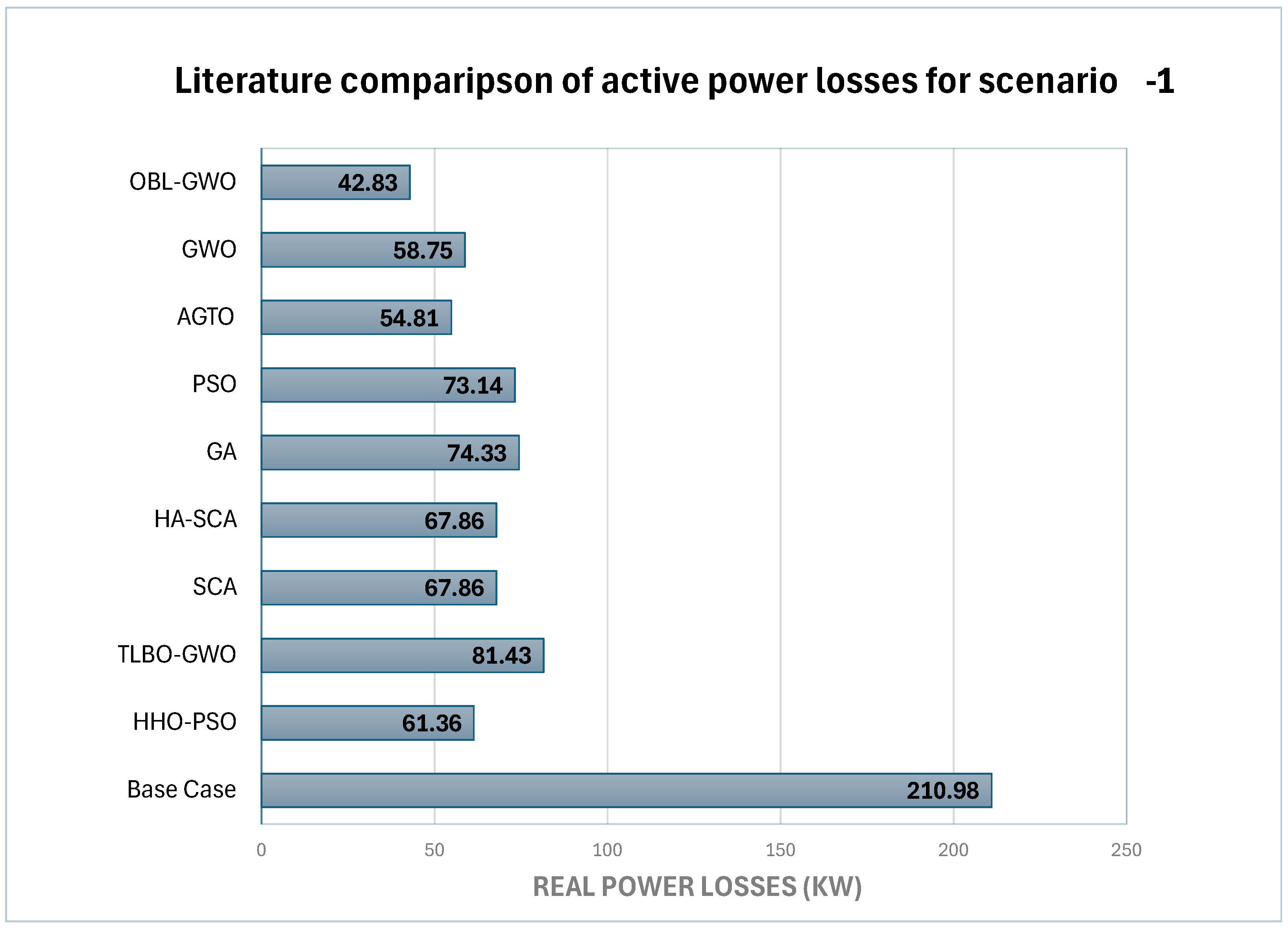
Because the OBL-augmented GWO maintains variety in the search process and prevents premature algorithm convergence, with respect to optimal DG allocation, the proposed OBL-GWO approach also outperformed other methods reported in published studies conducted under similar conditions. For Scenario 1, the OBL-GWO algorithm significantly improved the voltage profile and reduced total power losses on the IEEE 33-bus test system by involving a single WTG unit injecting active and reactive power at the optimal power factor (OPF), as shown in Table 11 and Figure 15. Although TVD and VSI values are not included due to a lack of reference data in the literature, the results clearly show that OBL-GWO outperformed conventional and advanced metaheuristic techniques such as GA, PSO, and SCA. Across all scenarios, the proposed method consistently achieved better technical performance, confirming its robustness and effectiveness in solving complex multi-objective optimization problems in active distribution networks. The accompanying tables and figures offer detailed numerical and visual comparisons with benchmark methods from the literature.

7.5. Stability Analysis Under Random Seeds and Extreme Conditions

To confirm robustness, the optimization was repeated with several random seeds affecting both load noise (with zero-mean variability) and algorithm initialization. The main results (power losses, voltage profiles, and VSI values) showed only small variations, and the ranking of scenarios remained unchanged. In addition, stress tests with ±20% to cover rare extreme demand scenarios were performed. In all cases, the algorithm converged successfully, and the improvements in loss reduction, voltage stability, and VSI were consistent, confirming that the conclusions are stable under different seeds and operating extremes. Figure 16 depicts the seasonal load profiles with different seeds, ±20% stress test cases, and zero-mean variability.
It should be noted that this study has several limitations. The power factor was modeled as fixed rather than time-varying, which could affect dynamic dispatch realism. In addition, only one turbine model (GE 1.5sle) and a single test feeder (IEEE 33-bus) were used for validation. Future work could extend the framework to time-varying PF schedules, alternative turbine technologies, and larger or meshed distribution networks. Furthermore, this study is limited to specific technical objectives, whereas other important aspects such as economic costs, social acceptance, and environmental impacts are equally crucial for comprehensive planning.

8. Conclusions

Successful planning must consider stochastic weather-contingent REG and seasonal demand. A useful, newly developed five-year database provides actual wind speed and load consumption statistics. Three scenarios with varied WTG integration were tested on the IEEE 33-bus system to obtain exploration and premature convergence results under both conventional GWO and OBL-augmented GWO. Optimal OBL-GWO DG placements led to decreased P l o s s and TVD. While only nominally enhanced, VSI and V m i n were invariably unrivaled under very different parameters and DG installations. The proposed approach also surpassed other methods across the board with respect to Ploss, TVD, VSI, and V m i n . The findings testify to the contribution of the new technique as significant progress in vital efforts to incorporate green REG into today’s networks. The framework promotes resilient, cost-effective, sustainable electricity networks that can meet burgeoning demand, safeguard grid stability, and manifest soundness and practicality in unraveling complicated optimization challenges. OBL-GWO could also assist with co-optimizing WTG-based DGs and EVCSs, incorporating unpredictable EV charging profiles into probabilistic load frameworks and evaluating the collective effect on power losses and voltage stability for large-scale DNs.

Author Contributions

Conceptualization, A.A. and A.D.; methodology, A.A.; software, A.A.; validation, A.A. and A.D.; formal analysis, A.A.; investigation, A.A.; resources, A.A. and A.D.; data curation, A.A.; writing—original draft preparation, A.A. and A.D.; writing—review and editing, A.A. and A.D.; visualization, A.A.; supervision, A.D.; project administration, A.D.; funding acquisition, A.D. All authors have read and agreed to the published version of the manuscript.

Funding

This research received no external funding.

Institutional Review Board Statement

Not applicable.

Informed Consent Statement

Not applicable.

Data Availability Statement

The IEEE 33-bus test system data are publicly available. The processed load demand data were obtained in collaboration with the Saudi Electricity Company (SEC) and cannot be shared publicly due to confidentiality agreements. The wind speed datasets used in this study were obtained from the Meteoblue website (https://www.meteoblue.com) and are available from the corresponding author upon reasonable request.

Conflicts of Interest

The authors declare no conflicts of interest.

Abbreviations

ACSAnt Colony System
ANDActive Distribution Network
AHPAnalytic Hierarchy Process
BESBattery Energy Storage
BESSBattery Energy Storage Systems
CBCapacitor Banks
DEDifferential Evolution
DGDistributed Generations
DNDistribution Networks
DRDemand Response
EPExpectation Propagation
ESEnvelope Strategy
GAGenetic Algorithms
GISGeographic Information System
GSAGravitational Search Algorithm
GWOGrey Wolf Optimization
NRNetwork Reconfiguration
OBLOpposition-Based Learning
RDNRadial Distribution Network
REGRenewable Energy Generation
RESRenewable Energy Sources
SASimulated Annealing
TVDTotal Voltage Deviation
VVOVolt-Var Optimization
VSIVoltage Stability Index
WTGWind Turbine Generator

References

  1. Yuvaraj, T.; Devabalaji, K.R.; Thanikanti, S.B.; Aljafari, B.; Nwulu, N. Minimizing the Electric Vehicle Charging Stations Impact in the Distribution Networks by Simultaneous Allocation of DG and DSTATCOM with Considering Uncertainty in Load. Energy Rep. 2023, 10, 1796–1817. [Google Scholar] [CrossRef]
  2. Dharavat, N.; Sudabattula, S.K.; Velamuri, S.; Mishra, S.; Sharma, N.K.; Bajaj, M.; Elgamli, E.; Shouran, M.; Kamel, S. Optimal Allocation of Renewable Distributed Generators and Electric Vehicles in a Distribution System Using the Political Optimization Algorithm. Energies 2022, 15, 6698. [Google Scholar] [CrossRef]
  3. Gao, H.; Diao, R.; Zhong, Y.; Zeng, R.; Wu, Q.; Jin, S. Optimal Allocation of Distributed Generation in Active Distribution Power Network Considering HELM-Based Stability Index. Int. J. Electr. Power Energy Syst. 2024, 155, 109508. [Google Scholar] [CrossRef]
  4. Balu, K.; Mukherjee, V. Optimal Allocation of Electric Vehicle Charging Stations and Renewable Distributed Generation with Battery Energy Storage in Radial Distribution System Considering Time Sequence Characteristics of Generation and Load Demand. J. Energy Storage 2023, 59, 106533. [Google Scholar] [CrossRef]
  5. Suresh, M.P.; Yuvaraj, T.; Thanikanti, S.B.; Nwulu, N. Optimizing Smart Microgrid Performance: Integrating Solar Generation and Static VAR Compensator for EV Charging Impact, Emphasizing SCOPE Index. Energy Rep. 2024, 11, 3224–3244. [Google Scholar] [CrossRef]
  6. Zeb, M.Z.; Imran, K.; Khattak, A.; Janjua, A.K.; Pal, A.; Nadeem, M.; Zhang, J.; Khan, S. Optimal Placement of Electric Vehicle Charging Stations in the Active Distribution Network. IEEE Access 2020, 8, 68124–68134. [Google Scholar] [CrossRef]
  7. Casella, V.; Fernandez Valderrama, D.; Ferro, G.; Minciardi, R.; Paolucci, M.; Parodi, L.; Robba, M. Towards the Integration of Sustainable Transportation and Smart Grids: A Review on Electric Vehicles’ Management. Energies 2022, 15, 4020. [Google Scholar] [CrossRef]
  8. Yu, H.; Niu, S.; Shang, Y.; Shao, Z.; Jia, Y.; Jian, L. Electric Vehicles Integration and Vehicle-to-Grid Operation in Active Distribution Grids: A Comprehensive Review on Power Architectures, Grid Connection Standards and Typical Applications. Renew. Sustain. Energy Rev. 2022, 168, 112812. [Google Scholar] [CrossRef]
  9. Hai, T.; Zhou, J.; Alazzawi, A.K.; Muranaka, T. Management of Renewable-Based Multi-Energy Microgrids with Energy Storage and Integrated Electric Vehicles Considering Uncertainties. J. Energy Storage 2023, 60, 106582. [Google Scholar] [CrossRef]
  10. Chakraborty, A.; Ray, S. Optimal Allocation of Distribution Generation Sources with Sustainable Energy Management in Radial Distribution Networks Using Metaheuristic Algorithm. Comput. Electr. Eng. 2024, 116, 109142. [Google Scholar] [CrossRef]
  11. Tercan, S.M.; Demirci, A.; Unutmaz, Y.E.; Elma, O.; Yumurtaci, R. A Comprehensive Review of Recent Advances in Optimal Allocation Methods for Distributed Renewable Generation. IET Renew Power Gen. 2023, 17, 3133–3150. [Google Scholar] [CrossRef]
  12. Yuvaraj, T.; Devabalaji, K.R.; Kumar, J.A.; Thanikanti, S.B.; Nwulu, N.I. A Comprehensive Review and Analysis of the Allocation of Electric Vehicle Charging Stations in Distribution Networks. IEEE Access 2024, 12, 5404–5461. [Google Scholar] [CrossRef]
  13. Sharma, P.; Raju, S. Metaheuristic Optimization Algorithms: A Comprehensive Overview and Classification of Benchmark Test Functions. Soft Comput. 2024, 28, 3123–3186. [Google Scholar] [CrossRef]
  14. Madhusudhan, M.; Kumar, N.; Pradeepa, H. Optimal Location and Capacity of DG Systems in Distribution Network Using Genetic Algorithm. Int. J. Inf. Tecnol. 2021, 13, 155–162. [Google Scholar] [CrossRef]
  15. Ahmad, F.; Bilal, M. Allocation of Plug-in Electric Vehicle Charging Station with Integrated Solar Powered Distributed Generation Using an Adaptive Particle Swarm Optimization. Electr. Eng. 2024, 106, 2595–2608. [Google Scholar] [CrossRef]
  16. Ahmadi, B.; Younesi, S.; Ceylan, O.; Ozdemir, A. An Advanced Grey Wolf Optimization Algorithm and Its Application to Planning Problem in Smart Grids. Soft Comput. 2022, 26, 3789–3808. [Google Scholar] [CrossRef]
  17. Mirjalili, S.; Mirjalili, S.M.; Lewis, A. Grey Wolf Optimizer. Adv. Eng. Softw. 2014, 69, 46–61. [Google Scholar] [CrossRef]
  18. Wang, Z.; Dai, D.; Zeng, Z.; He, D.; Chan, S. Multi-Strategy Enhanced Grey Wolf Optimizer for Global Optimization and Real World Problems. Clust. Comput. 2024, 27, 10671–10715. [Google Scholar] [CrossRef]
  19. Ansari, M.M.; Guo, C.; Shaikh, M.S.; Chopra, N.; Haq, I.; Shen, L. Planning for Distribution System with Grey Wolf Optimization Method. J. Electr. Eng. Technol. 2020, 15, 1485–1499. [Google Scholar] [CrossRef]
  20. Ahmad, F.; Iqbal, A.; Ashraf, I.; Marzband, M.; Khan, I. Placement of Electric Vehicle Fast Charging Stations Using Grey Wolf Optimization in Electrical Distribution Network. In Proceedings of the 2022 IEEE International Conference on Power Electronics, Smart Grid, and Renewable Energy (PESGRE), Trivandrum, India, 2 January 2022; pp. 1–6. [Google Scholar]
  21. Sultana, U.; Khairuddin, A.B.; Mokhtar, A.S.; Zareen, N.; Sultana, B. Grey Wolf Optimizer Based Placement and Sizing of Multiple Distributed Generation in the Distribution System. Energy 2016, 111, 525–536. [Google Scholar] [CrossRef]
  22. Jordehi ARezaee, D.G. Allocation and Reconfiguration in Distribution Systems by Metaheuristic Optimisation Algorithms: A Comparative Analysis. In Proceedings of the 2018 IEEE PES Innovative Smart Grid Technologies Conference Europe (ISGT-Europe), Sarajevo, Bosnia and Herzegovina, 21–25 October 2018; pp. 1–6. [Google Scholar]
  23. Long, W.; Jiao, J.; Liang, X.; Tang, M. Inspired Grey Wolf Optimizer for Solving Large-Scale Function Optimization Problems. Appl. Math. Model. 2018, 60, 112–126. [Google Scholar] [CrossRef]
  24. Saremi, S.; Mirjalili, S.Z.; Mirjalili, S.M. Evolutionary Population Dynamics and Grey Wolf Optimizer. Neural Comput. Appl. 2015, 26, 1257–1263. [Google Scholar] [CrossRef]
  25. Heidari, A.A.; Pahlavani, P. An Efficient Modified Grey Wolf Optimizer with Lévy Flight for Optimization Tasks. Appl. Soft Comput. 2017, 60, 115–134. [Google Scholar] [CrossRef]
  26. Rodríguez, L.; Castillo, O.; Soria, J.; Melin, P.; Valdez, F.; Gonzalez, C.I.; Martinez, G.E.; Soto, J. A Fuzzy Hierarchical Operator in the Grey Wolf Optimizer Algorithm. Appl. Soft Comput. 2017, 57, 315–328. [Google Scholar] [CrossRef]
  27. Long, W.; Wu, T.; Cai, S.; Liang, X.; Jiao, J.; Xu, M. A Novel Grey Wolf Optimizer Algorithm with Refraction Learning. IEEE Access 2019, 7, 57805–57819. [Google Scholar] [CrossRef]
  28. Kumar, V.; Kumar, D. An Astrophysics-Inspired Grey Wolf Algorithm for Numerical Optimization and Its Application to Engineering Design Problems. Adv. Eng. Softw. 2017, 112, 231–254. [Google Scholar] [CrossRef]
  29. Ibrahim, R.A.; Elaziz, M.A.; Lu, S. Chaotic Opposition-Based Grey-Wolf Optimization Algorithm Based on Differential Evolution and Disruption Operator for Global Optimization. Expert. Syst. Appl. 2018, 108, 1–27. [Google Scholar] [CrossRef]
  30. Long, W.; Jiao, J.; Liang, X.; Tang, M. An Exploration-Enhanced Grey Wolf Optimizer to Solve High-Dimensional Numerical Optimization. Eng. Appl. Artif. Intell. 2018, 68, 63–80. [Google Scholar] [CrossRef]
  31. Gupta, S.; Deep, K. A Novel Random Walk Grey Wolf Optimizer. Swarm Evol. Comput. 2019, 44, 101–112. [Google Scholar] [CrossRef]
  32. Yu, X.; Xu, W.; Li, C. Opposition-Based Learning Grey Wolf Optimizer for Global Optimization. Knowl. Based Syst. 2021, 226, 107139. [Google Scholar] [CrossRef]
  33. Bansal, J.C.; Singh, S. A Better Exploration Strategy in Grey Wolf Optimizer. J. Ambient. Intell. Hum. Comput. 2021, 12, 1099–1118. [Google Scholar] [CrossRef]
  34. Alomoush, A.A.; Alsewari, A.A.; Alamri, H.S.; Aloufi, K.; Zamli, K.Z. Hybrid Harmony Search Algorithm with Grey Wolf Optimizer and Modified Opposition-Based Learning. IEEE Access 2019, 7, 68764–68785. [Google Scholar] [CrossRef]
  35. Long, W.; Jiao, J.; Liang, X.; Cai, S.; Xu, M. A Random Opposition-Based Learning Grey Wolf Optimizer. IEEE Access 2019, 7, 113810–113825. [Google Scholar] [CrossRef]
  36. Chandran, V.; Mohapatra, P. Enhanced Opposition-Based Grey Wolf Optimizer for Global Optimization and Engineering Design Problems. Alex. Eng. J. 2023, 76, 429–467. [Google Scholar] [CrossRef]
  37. Li, X.; Yu, T.; Zhang, F.; Huang, J.; He, D.; Chu, F. Mixed Style Network Based: A Novel Rotating Machinery Fault Diagnosis Method through Batch Spectral Penalization. Reliab. Eng. Syst. Saf. 2025, 255, 110667. [Google Scholar] [CrossRef]
  38. Li, X.; Xiao, S.; Li, Q.; Zhu, L.; Wang, T.; Chu, F. The Bearing Multi-Sensor Fault Diagnosis Method Based on a Multi-Branch Parallel Perception Network and Feature Fusion Strategy. Reliab. Eng. Syst. Saf. 2025, 261, 111122. [Google Scholar] [CrossRef]
  39. Zhi, S.; Su, K.; Yu, J.; Li, X.; Shen, H. An Unsupervised Transfer Learning Bearing Fault Diagnosis Method Based on Multi-Channel Calibrated Transformer with Shiftable Window. Struct. Health Monit. 2025. [Google Scholar] [CrossRef]
  40. Li, X.; Yu, T.; Wang, X.; Li, D.; Xie, Z.; Kong, X. Fusing Joint Distribution and Adversarial Networks: A New Transfer Learning Method for Intelligent Fault Diagnosis. Appl. Acoust. 2024, 216, 109767. [Google Scholar] [CrossRef]
  41. Historical Weather Data Download. Available online: https://www.meteoblue.com/en/weather/archive/export (accessed on 28 September 2024).
  42. Manwell, J.F. Wind Energy Explained: Theory, Design and Application; Wiley: Hoboken, NJ, USA, 2009. [Google Scholar]
  43. Gao, F.; Yuan, C.; Li, Z.; Zhuang, S. Multi-Objective Optimal Allocation of Distributed Generation Considering the Spatiotemporal Correlation of Wind-Photovoltaic-Load. Electr. Power Syst. Res. 2023, 214, 108914. [Google Scholar] [CrossRef]
  44. Sharaf, A.M.; El-Gammal, A.A.A. A Novel PSO-Based Hybrid PV-FC-Diesel-Battery Electric PID-Controller Drive System for Electric Vehicle Traction. In Proceedings of the 2010 IEEE Electrical Power & Energy Conference, Halifax, NS, Canada, 25–27 August 2010; pp. 1–6. [Google Scholar]
  45. Hasan, S.; Alaqeel, T.; Peerbocus, N. Saudi Arabia’s Unfolding Power Sector Reform: Features, Challenges and Opportunities for Market Integration; King Abdullah Petroleum Studies and Research Center: Riyadh, Saudi Arabia, 2020. [Google Scholar]
  46. Fioriti, D.; Poli, D.; Duenas-Martinez, P.; Perez-Arriaga, I. Multi-Year Stochastic Planning of off-Grid Microgrids Subject to Significant Load Growth Uncertainty: Overcoming Single-Year Methodologies. Electr. Power Syst. Res. 2021, 194, 107053. [Google Scholar] [CrossRef]
  47. Oda, E.S.; Abd El Hamed, A.M.; Ali, A.; Elbaset, A.A.; Abd El Sattar, M.; Ebeed, M. Stochastic Optimal Planning of Distribution System Considering Integrated Photovoltaic-Based DG and DSTATCOM Under Uncertainties of Loads and Solar Irradiance. IEEE Access 2021, 9, 26541–26555. [Google Scholar] [CrossRef]
  48. Ehsan, A.; Yang, Q. Optimal Integration and Planning of Renewable Distributed Generation in the Power Distribution Networks: A Review of Analytical Techniques. Appl. Energy 2018, 210, 44–59. [Google Scholar] [CrossRef]
  49. Ouafa, H.; Linda, S.; Tarek, B. Multi-Objective Optimal Power Flow Considering the Fuel Cost, Emission, Voltage Deviation and Power Losses Using Multi-Objective Dragonfly Algorithm. In Proceedings of the International Conference on Recent Advances in Electrical Systems, Hammamet, Tunisia, 22–24 December 2017. [Google Scholar]
  50. Venkatesan, C.; Kannadasan, R.; Alsharif, M.H.; Kim, M.-K.; Nebhen, J. A Novel Multiobjective Hybrid Technique for Siting and Sizing of Distributed Generation and Capacitor Banks in Radial Distribution Systems. Sustainability 2021, 13, 3308. [Google Scholar] [CrossRef]
  51. Elkadeem, M.R.; Abd Elaziz, M.; Ullah, Z.; Wang, S.; Sharshir, S.W. Optimal Planning of Renewable Energy-Integrated Distribution System Considering Uncertainties. IEEE Access 2019, 7, 164887–164907. [Google Scholar] [CrossRef]
  52. Garces, A. On the Convergence of Newton’s Method in Power Flow Studies for DC Microgrids. IEEE Trans. Power Syst. 2018, 33, 5770–5777. [Google Scholar] [CrossRef]
  53. Grisales-Noreña, L.F.; Montoya, O.D.; Gil-González, W.J.; Perea-Moreno, A.-J.; Perea-Moreno, M.-A. A Comparative Study on Power Flow Methods for Direct-Current Networks Considering Processing Time and Numerical Convergence Errors. Electronics 2020, 9, 2062. [Google Scholar] [CrossRef]
  54. Akbar, M.I.; Kazmi, S.A.A.; Alrumayh, O.; Khan, Z.A.; Altamimi, A.; Malik, M.M. A Novel Hybrid Optimization-Based Algorithm for the Single and Multi-Objective Achievement with Optimal DG Allocations in Distribution Networks. IEEE Access 2022, 10, 25669–25687. [Google Scholar] [CrossRef]
  55. Bilal, M.; Rizwan, M.; Alsaidan, I.; Almasoudi, F.M. AI-Based Approach for Optimal Placement of EVCS and DG With Reliability Analysis. IEEE Access 2021, 9, 154204–154224. [Google Scholar] [CrossRef]
  56. Arabi Nowdeh, S.; Davoudkhani, I.F.; Hadidian Moghaddam, M.J.; Najmi, E.S.; Abdelaziz, A.Y.; Ahmadi, A.; Razavi, S.E.; Gandoman, F.H. Fuzzy Multi-Objective Placement of Renewable Energy Sources in Distribution System with Objective of Loss Reduction and Reliability Improvement Using a Novel Hybrid Method. Appl. Soft Comput. 2019, 77, 761–779. [Google Scholar] [CrossRef]
  57. Selim, A.; Kamel, S.; Mohamed, A.A.; Elattar, E.E. Optimal Allocation of Multiple Types of Distributed Generations in Radial Distribution Systems Using a Hybrid Technique. Sustainability 2021, 13, 6644. [Google Scholar] [CrossRef]
  58. Tiwari, V.; Dubey, H.M.; Pandit, M. Assessment of Optimal Size and Location of DG/CB in Distribution Systems Using Coulomb–Franklin’s Algorithm. J. Inst. Eng. India Ser. B 2022, 103, 1885–1908. [Google Scholar] [CrossRef]
  59. Roy, K.; Bansal, S.K.; Bansal, R.C. Performance Enhancement of Radial Distribution System with Optimal DG Allocation. Int. J. Model. Simul. 2025, 45, 245–263. [Google Scholar] [CrossRef]
Figure 1. Stages of the developed framework and resultant benefits.
Sustainability 17 08819 g001
Figure 2. Historical variations in seasonal wind speeds across four seasons.
Sustainability 17 08819 g002
Figure 3. Modeling results indicating wind speed variations across four seasons.
Sustainability 17 08819 g003
Figure 4. Normalized hourly demand profiles for a sample day in each season.
Sustainability 17 08819 g004
Figure 5. Post-modeling 96 h Riyadh seasonal load profile.
Sustainability 17 08819 g005
Figure 6. Schematic of an RDN.
Sustainability 17 08819 g006
Figure 7. IEEE 33-bus test system schematic.
Sustainability 17 08819 g007
Figure 8. DN radial system schematic.
Sustainability 17 08819 g008
Figure 9. Base case voltages at each bus in the test system.
Sustainability 17 08819 g009
Figure 10. Seasonal voltage profiles with GWO applied for varied numbers of DGs embedded in the IEEE 33-bus test system shown in per-unit on a base of 3.715 MVA and 12.66 kV: (a) Scenario 1: one WTG unit; (b) Scenario 2: two WTG units; (c) Scenario 3: three WTG units.
Sustainability 17 08819 g010
Figure 11. DN scheme for use with the OBL-GWO approach.
Sustainability 17 08819 g011
Figure 12. IEEE-33 test system voltage profiles for each season obtained with the OBL-GWO method shown in per-unit on a base of 3.715 MVA and 12.66 kV: (a) Scenario 1 (one WTG unit); (b) Scenario 2 (two WTG units); (c) Scenario 3, (three WTG units).
Sustainability 17 08819 g012
Figure 13. Convergence curves of the conventional GWO and the proposed OBL-GWO algorithm for all scenarios.
Sustainability 17 08819 g013
Figure 14. Convergence curves (median ± IQR over 30 independent runs) for GWO and OBL-GWO in Scenario 2.
Sustainability 17 08819 g014
Figure 15. Literature comparison of active power losses for Scenario 1. Results of the proposed methods (OBL-GWO and GWO) are compared with other approaches reported in the literature, including AGTO [59], PSO [58], GA [58], HA-SCA [57], SCA [57], TLBO-GWO [56], and HHO-PSO [51].
Sustainability 17 08819 g015
Figure 16. Seasonal base load modeling with stability analysis used for validation.
Sustainability 17 08819 g016
Table 1. Comparison of this study with related OBL-GWO variants in the literature.
Reference/YearDomainUncertainty ModelingLoad-Growth ConsideredDatasetPerformance MetricsBaseline MethodsKey Contribution/Limitation
[35]/2019Global optimization and engineering testsNoneN/A23–30 benchmark problemsbest/mean/stdDiverse metaheuristicsAdds random OBL to improve exploration; no DN modeling.
[34]/2019Feature selection/global optimizationNoneN/ABenchmark setsaccuracy/fitnessHS, GWO variantsHybrid HS + GWO with OBL; outside DG/ADN context.
[32]/2021Generic global optimization (benchmarks)Only deterministic functionsN/AStandard test functionsbest/mean/std, convergencePSO/DE/GSA etc.Introduces OGWO with OBL; not power-system specific.
[36]/2023Global optimization and engineering designNoneN/AEngineering design setsbest/mean/stdMany heuristicsPerformance-enhanced OBL-GWO; not DN/uncertainty focused.
[P]/2025WTG-DG siting and sizing in an ADN (IEEE-33)Seasonal stochasticity for wind (Weibull) + stochastic load noise; 5-year real dataYes: multi-year demand growth (5.48%/yr over 20 y)5-year measured wind and load (for Riyadh), seasonal 96 h blocks P loss ,   TVD ,   VSI ,   V m i n ; convergenceStandard GWO; plus, GA/PSO/SCA, etc., from literatureApplies OBL-GWO to WTG-DG allocation under real seasonal variability + growth; validates on IEEE-33 and benchmarks against published methods.
[P]—the proposed method presented in this study.
Table 3. Seasonal Weibull parameters for wind speed modeling.
Seasonk (Shape)95% CI (k) c (Scale) 95 %   CI (c)
Spring1.8764[1.3757–2.5591]5.4763[4.3689–6.8643]
Summer2.7687[2.0379–3.7614]6.654[5.7101–7.7539]
Autumn3.0124[2.1682–4.1854]5.3766[4.6765–6.1816]
Winter3.1054[2.2651–4.2573]6.3097[5.5078–7.2284]
Table 4. Tested weight sets for the multi-objective function.
Weight Set(Ploss, Qloss, TVD, VSI)Main Observation
Equal (default)(0.25, 0.25, 0.25, 0.25)Balanced trade-off; used in all main results
Loss-focused(0.40, 0.40, 0.10, 0.10)Slightly lower losses, but same optimal buses
Stability-focused(0.10, 0.10, 0.40, 0.40)Slightly higher VSI, but unchanged scenario ranking
Table 5. IEEE 33-bus test system parameters.
System ParameterValue
Number   of   buses   ( N b u s ) 33
Number   of   branches   ( N b r ) 32
Nominal   voltage   ( kV ) 12.66
MVA base 100
S l o a d (MVA) 3.715 + j 2.300
Table 6. Base case simulation outcomes (no DG).
Performance MetricSimulated Value
P l o s s (kW) 210.07
Q l o s s (kVAr) 142.43
TVD (p.u.) 0.1328
VSI (p.u.) 0.705
V m i n (p.u.) 0.9072
Table 7. Optimization setup and reproducibility parameters.
ParameterValue/Description
Maximum iterations200
Population size100 search agents
Randomization policy30 independent runs with different random seeds
Stopping criteriaMaximum iterations
OBL injection policyApplied every iteration (100% rate)
DG size limits (kVA)0 ≤ S_DG ≤ 3000
DG power factor limits0.9 ≤ PF ≤ 1.0
Simulation environmentMATLAB R2022a, Apple M1 Pro, 16 GB RAM, macOS Sonoma 14.5
Table 8. Multi-objective GWO and OBL-GWO outcomes for all scenarios.
MethodScenarioOptimal LocationsOptimal Sizing%DG PenetrationPower LossesTVDVSI V m i n
P (kW)Q (kvar)Ploss (kW)p.u.p.u.p.u.
-Base Case----210.070.13280.7050.9072 (18)
GWOScenario 1821451534.5071.6%58.750.00860.87810.9671 (18)
Scenario 213850789.3375.2%38.90.00230.91720.9749 (18)
301300979.50
Scenario 3311200462.7895.4%18.630.000590.96770.9727 (33)
25821504.73
32940893.39
OBL-GWOScenario 1623171923.4081.4%42.830.00480.91350.9717 (18)
Scenario 23218201210.2799.2%22.590.00170.96730.9897 (33)
61250864.23
Scenario 330923.12513.2394.1%10.220.000310.99820.9947 (25)
131378.23620.23
25115.24913.56
Table 9. Statistical performance over 30 independent runs of GWO and OBL-GWO.
MethodMetricBestWorstMean ± Std
GWO P l o s s (kW)36.841.238.9 ± 1.5
TVD (p.u.)0.00160.00190.0017 ± 0.0001
VSI (p.u.)0.9130.9210.9172 ± 0.003
V m i n (p.u.)0.97250.97650.9749 ± 0.0015
OBL-GWO P l o s s (kW)21.923.522.6 ± 0.6
TVD (p.u.)0.00220.00240.0023 ± 0.0001
VSI (p.u.)0.9650.970.9673 ± 0.002
V m i n (p.u.)0.9880.9910.9897 ± 0.0015
Table 10. Performance metrics comparisons for base case, GWO, and OBL-GWO under Scenarios 1–3.
ScenarioMethod/ImprovementsPloss (kW)TVD (p.u.)VSI (p.u.) V m i n (p.u.)
Base Case-210.070.13280.7050.9072
Scenario 1GWO58.750.00860.87810.9671
Improvements vs. Base72.03%93.52%+24.55%+6.60%
OBL-GWO42.830.00480.91350.9717
Improvements vs. Base79.61%96.39%+29.57%7.11%
Improvements vs. GWO27.1%44.19%+4.03%+0.48%
Scenario 2GWO38.90.00230.91720.9749
Improvements vs. Base81.48%98.27%+30.10%+7.46%
OBL-GWO22.590.00170.96730.9897
Improvements vs. Base89.25%98.72%+37.21%+9.09%
Improvements vs. GWO41.93%26.09%+5.46%1.52%
Scenario 3GWO18.630.000590.96770.9727
Improvements vs. Base91.13%99.56%+37.26%+7.22%
OBL-GWO10.220.000310.99820.9947
Improvements vs. Base95.13%99.77%+41.59%+9.65%
Improvements vs. GWO45.14%47.46%+3.15%+2.26%
Table 11. Results using the proposed approach compared with those produced by existing methods for Scenario 1 1.
Method/ReferenceYearOptimal LocationsOptimal SizingReal Power LossesOPF V m i n (p.u.)
P (kW)Q (var)Ploss (kW)Qloss (kvar)
Base Case----210.98-0.820.9038 (18)
HHO-PSO [51]2019630882155.4361.36-0.800.9557 (18)
TLBO-GWO [56]2019301000750.0081.43-0.820.9558 (18)
SCA [57]202162546.81777.6867.86-0.820.9510 (18)
HA-SCA [57]202162546.7151777.6267.86-0.84-
GA [58]202263025.11954.0074.3355.940.830.9424 (18)
PSO [58]202262888.11940.8073.1454.860.840.9424 (18)
AGTO [59]202562541.71775.267.8754.810.820.9580 (18)
GWO [P]202582420.31534.5058.7558.750.860.9671 (18)
OBL_GWO [P]202563250.71923.4042.8342.830.820.9717 (18)
1 Table Abbreviations: HHO-PSO: Harris Hawks Optimizer–Particle Swarm Optimization; TLBO-GWO: Teaching–Learning-Based Optimization–Grey Wolf Optimizer; SCA: Sine Cosine Algorithm; HA-SCA: Hybrid Analytical Sine Cosine Algorithm; GA: Genetic Algorithm; PSO: Particle Swarm Optimization; AGTO: Artificial Gorilla Troops Optimizer. [P]—the proposed method presented in this study.
Disclaimer/Publisher’s Note: The statements, opinions and data contained in all publications are solely those of the individual author(s) and contributor(s) and not of MDPI and/or the editor(s). MDPI and/or the editor(s) disclaim responsibility for any injury to people or property resulting from any ideas, methods, instructions or products referred to in the content.