Article

Spatial–Environmental Coupling and Sustainable Planning of Traditional Tibetan Villages: A Case Study of Four Villages in Suopo Township

by
Zhe Lei
,
Weiran Han
and
Junhuan Li
*
School of Architecture, Xi’an University of Architecture and Technology, Yanta Street, Xi’an 710055, China
*
Author to whom correspondence should be addressed.
Sustainability 2025, 17(19), 8766; https://doi.org/10.3390/su17198766
Submission received: 22 July 2025 / Revised: 11 September 2025 / Accepted: 24 September 2025 / Published: 30 September 2025
(This article belongs to the Section Sustainable Urban and Rural Development)

Abstract

Mountain settlements represent culturally rich but environmentally fragile landscapes, shaped by enduring processes of ecological adaptation and human resilience. In western Sichuan, Jiarong Tibetan villages, with their distinctive integration of defensive stone towers and settlements, embody this coupling of culture and the environment. We hypothesize that settlement cores in these villages were shaped by natural environmental factors, with subsequent expansion reinforced by the cultural significance of towers. To test this, we applied a micro-scale spatial–environmental framework to four sample villages in Suopo Township, Danba County. High-resolution World Imagery (Esri, 0.5–1 m, 2022–2023) was classified via a Random Forest algorithm to generate detailed land-use maps, and a 100 × 100 m fishnet grid extracted topographic metrics (elevation, slope, aspect) and accessibility measures (distances to streams, roads, towers). Geographically weighted regression (GWR) was then used to examine how slope, elevation, aspect, proximity to water and roads, and tower distribution affect settlement patterns. The results show built-up density peaks on southeast-facing slopes of 15–30°, at altitudes of 2600–2800 m, and within 50–500 m of streams, co-locating with historic watchtower sites. Based on these findings, we propose four zoning strategies—a Core Protected Zone, a Construction And Development Zone, an Ecological Conservation Zone, and an Industry Development Zone—to balance preservation with growth. The resulting policy recommendations offer actionable guidance for sustaining traditional settlements in complex mountain environments.

1. Introduction

Mountain regions have emerged as critical frontiers for sustainable development in the face of environmental change and cultural transformation [1,2]. High-altitude settlements provide essential ecosystem services and support diverse cultural practices. However, these settlements are particularly susceptible to environmental disturbances [3,4].
In the mountainous regions of western Sichuan, Jiarong Tibetan villages are renowned for their distinctive cultural landscapes, reflecting UNESCO’s “combined works of nature and man” and forming important components of global heritage [5,6,7]. Shaped by the Hengduan Mountains’ high-altitude valleys and Bon religious culture, these villages follow a layout “backed by holy peaks, with watchtowers interwoven among dwellings”. Geographically, most of these villages lie in fragile ecosystems with limited arable land, exposed to extreme plateau climates and natural hazards [8]. Over the centuries, Jiarong Tibetan communities developed adaptive livelihood strategies—blending nomadic pastoralism with farming under communal and religious guidance—to sustainably manage these harsh environments [8].
However, today these unique villages confront mounting pressures from rapid urbanization and tourism industries [9]. This accelerated development has intensified competition for scarce land resources, exacerbating ecological vulnerabilities and compromising essential environmental services [9]. Furthermore, demographic shifts, characterized by the population exodus towards urban centers, coupled with the proliferation of modern lifestyles, have disrupted the traditional spatial cohesion of these settlements [6,10]. As a result, the intricate and historically evolved landscape inheritance chains are becoming fragmented, threatening the continuity of local heritage. This combination of ecological fragility and cultural erosion underscores the urgency and complexity of pursuing sustainable development within Tibetan villages in western Sichuan. Effective solutions require combining ecological restoration with cultural preservation to ensure both a healthy ecosystem and the continuation of traditions.
A central challenge is unraveling spatial–environmental coupling—the dynamic link between the village form and the surrounding landscape. In these communities, settlement patterns mirror environmental factors such as topography, climate, water sources, and natural resources [11]. Studies show that distinct topography, climate, and resource endowments produce unique “natural textures” for rural habitation, which in turn shape how villages grow and how their cultural landscapes are maintained [12]. In essence, the spatial organization of these heritage settlements reflects centuries of co-evolution between human communities and their environment—an inseparable blend of the cultural landscape and ecology [13,14]. It is recognized that this synergy is essential for preserving village authenticity and for designing planning measures that honor both ecological integrity and cultural legacy [15]. Recently, researchers have advanced studies on rural–environment interactions and developed sustainable-development frameworks for these villages.
Research has examined both natural (topography, geomorphology, hydrology, ecology) and human (socio-economic, cultural, policy) drivers of settlement patterns. Topography and hydrology dominate: Xu et al. link slope and altitude to village layout [4]; Li et al. highlight economic, climatic, and multi-factor influences in Jiarong Tibetan areas [10]; Liu et al. reveal that the relief degree of surface limits population clustering [16]; Li et al. explain the relationship between topographic variation and settlement patterns [17]. Additionally, water distribution and ecosystem services shape settlement structure [18,19]. Urbanization and rural revitalization policies also strongly drive the spatial reorganization of settlements [20,21]. At the same time, Peng et al. and Wang et al. proposed that cultural factors such as traditional feng shui theories and clan beliefs can profoundly impact traditional settlement site selection and layout [22,23].
Spatial statistical approaches like kernel density estimation, Ripley’s K-function, and the nearest-neighbor index are commonly used to analyze how rural settlements cluster and relate to environmental factors [3,4,17]. Measures like Moran’s I often reveal how settlement patterns correlate with environmental factors such as slope, elevation, and road density [4,24]. To examine local heterogeneity, regression approaches—such as binary logistic regression and geographically weighted regression (GWR)—are employed to quantify the influence of environmental and socio-economic factors on spatial patterns [25,26]. Multiscale Geographically Weighted Regression (MGWR) has also been adopted to reveal differentiated driving forces across spatial scales [27]. In addition, GeoDetector is now widely used to assess how individual environmental factors shape settlement distributions [28,29], often combined with AHP for more robust spatial-suitability analyses [29]. Advances in remote sensing and spatial data have enabled Random Forest classification to map settlement patches and model environmental impacts on rural land change [30,31]. Scenario models like CA-Markov and CLUE-S simulate future settlement landscapes under varied policy and ecological scenarios [25]. Together, these tools provide a layered methodology for both broad-scale forecasting and detailed, local insights into settlement–environment interactions.
Despite these advances, most studies focus on macro-scales or meso-scales, offering national or regional assessments. For instance, macro-scale studies usually examine provincial to national areas using data such as remote sensing imagery, population statistics, and land-use records, though these datasets have a fairly coarse spatial resolution [17,32,33,34]. Meso-scale research focuses on counties or cities, using detailed data—high-resolution satellite imagery, land surveys, and village-level socioeconomic statistics—to support local planning and management [35,36,37]. However, studies often pay little attention to the villages at the micro level [38]. And village studies often separate environmental and cultural aspects, examining architecture or land use instead of the coupled socio-environmental system. The recent literature emphasizes the need for more comprehensive frameworks. Jia et al. call for assessment tools that balance heritage conservation with rural revitalization [39], while Wu et al. (2025) urge the integration of resilience and cultural values into landscape evaluations [5]. In high-altitude heritage contexts, complex terrain and data scarcity further hinder fine-grained analysis, and few studies examine how settlement clusters adapt to extreme conditions [40].
Comparative research on sustainable development planning for mountainous rural areas beyond China shows a range of approaches. In Turkey’s Bursa region, Zeybek et al. used the Global Ecovillage Network Community Sustainability Assessment to evaluate the potential transformation of traditional villages, highlighting infrastructural and ecological challenges [41]. In Ethiopia’s Konso cultural landscape, studies show how climate variability interacts with terracing and indigenous institutions to sustain soil–water conservation and community resilience [42]. In the European Alps, Stotten et al. compared two villages and found that historical “lock-in” effects restrict adaptation, while more diversified communities are more resilient—emphasizing the need to consider path dependency in mountain planning [43]. In the Himalayas, Chaudhary et al. created a risk-based land-use planning framework that integrates topography and accessibility to map eco-environmental risks for high-mountain settlements in Nepal, demonstrating its value for areas facing farmland abandonment [44]. Zeballos-Velarde et al. examined the Colca Valley in Peru and showed how ancestral practices function as social capital that strengthens disaster resilience, underscoring the role of cultural traditions in mountain risk management [45]. Although these studies focus mainly on governance, risk management, or tourism, few link high-resolution spatial–environmental coupling directly to village-scale zoning, which underscores the contribution of this paper.
The contribution of this study lies less in the statistical method itself than in applying a data-driven spatial–environmental framework to fragile cultural landscapes and linking the results directly to zoning strategies for sustainable planning. In this way, the work responds to calls for more systematic analysis of village spatial organization that integrates both ecological and cultural dimensions into planning models [5,40]. While constrained by limited socio-economic data, the findings from Suopo offer an illustrative case that may inform sustainable development and conservation practices in Tibetan villages and other mountain settlements.
This study is guided by the hypothesis that the historical cores of settlement development in Suopo Township were shaped by natural environmental factors and that subsequent expansion has remained influenced by these conditions. Cultural heritage features, particularly the distribution of defensive stone towers, are also expected to reinforce these spatial patterns. To examine this, we introduce a high-resolution, micro-village perspective into settlement–environment coupling research. Using satellite-derived land-cover classification with field validation and a 100 m grid-based spatial framework, we analyze four traditional Tibetan villages in Suopo Township, Danba County. By integrating natural factors (elevation, slope, hydrology) with cultural elements (stone tower distribution) into a GWR model, we identify localized drivers of settlement distribution and form. While GWR has been widely applied to study spatial heterogeneity in urban and regional contexts, its use at the micro-scale of individual villages—particularly in remote, heritage-sensitive Tibetan mountain settings—remains relatively uncommon.
The objectives of this study are twofold. First, we aim to develop a micro-scale analytical framework that is capable of identifying how environmental and cultural variables shape settlement distribution in Tibetan villages. Second, we aim to link these findings to planning recommendations that balance conservation with appropriate development, through the delineation of four functional zones: Core Protection, Construction and Development, Ecological Conservation, and Industry Development. By situating micro-scale analysis within a broader planning discourse, this research seeks to advance the understanding of settlement–environment interactions while providing practical guidance for heritage conservation and rural revitalization in mountain regions.

2. Materials and Methods

2.1. Materials

Suopo Township lies in eastern Danba County, Garze Tibetan Autonomous Prefecture, Sichuan, nestled between the Dadu River Valley and snow-capped peaks at 1800–3200 m (Figure 1). Its distinct vertical climate zones exemplify the high-mountain gorges of the Hengduan Mountains. In Tibetan, “Suopo” means “Mongols”, recalling the Mongolian herders who once grazed here. During the Tang Dynasty, this region formed the heartland of the “Eastern Women’s Kingdom,” traces of which still endure. Today, Suopo preserves 172 ancient watchtowers—the densest concentration in China and beyond—listed as national key cultural relics in 2006 and attracting sustained government and academic attention.
Villages in Suopo cling to the Dadu Valley’s steep slopes, backed by mountains and fronting the river—terrain that is both arable and defensible. Winding roads follow natural contours, while houses and watchtowers interlock in staggered patterns, giving the settlement an organic growth form. Traditional dwellings are three- to four-story stone-and--wood structures, with livestock pens and storage on the ground floor and living and drying spaces above, reflecting a mixed farming and pastoral lifestyle. This study focuses on four contiguous villages—Xiala, Zegong, Zezhou, and Songda—on the west bank of the Dadu River within Suopo Township. Their settlement patterns closely mirror those of other high-altitude canyon villages in Danba County, making them exemplary case studies. Although they are officially four separate villages, these settlements have merged organically and now form a contiguous unit. Accordingly, this study treats them as a single entity, using their combined administrative boundaries as the analysis area. We perform a micro-level spatial–environmental coupling analysis—examining slope gradients, slope aspects, water systems, roads, and farmland—to uncover how these factors shape settlement siting and layout. This approach yields precise spatial controls and indicators to guide sustainable development planning.

2.2. Methods

This study employed a four-step framework. First, high-resolution imagery, DEM, OSM road and hydrology data, and UAV/GPS surveys were collected. Land-use types were classified using a Random Forest algorithm, reclassified, and validated. Second, a 100 × 100 m fishnet grid was used to quantify built-up and cropland areas, topographic factors (elevation, slope, aspect), and accessibility to water, roads, and towers. Third, spatial patterns were analyzed using Moran’s I, kernel density estimation, and convex mapping. Finally, OLS and GWR models identified the main driving factors, providing the basis for planning strategies (Figure 2).
The processing of high-resolution satellite imagery in mountainous, high-altitude regions poses several significant challenges. First, extensive cloud cover, especially persistent, thick clouds and snow cover, limits the availability of usable data. Second, image classification typically requires repeated training and calibration of models like Random Forest to achieve acceptable accuracy, including efforts to mitigate terrain shadowing and misclassifications. Third, to generate reliable, high-resolution land-cover maps, the output must undergo substantial post-processing, including the removal of misclassified and invalid grid cells, and conversion from raster to vector formats for spatial aggregation and analysis. Lastly, the need to harmonize multiple datasets—each with varying levels of resolution and positional accuracy—adds complexity to the workflow and demands meticulous geospatial integration. Data sources for the study area are shown in Table 1.

2.2.1. Land-Cover Classification

Training and Classification
The study began with a land-cover classification to define the major land-use categories in the study area. The data source was the 2024 World Imagery (Esri) high-resolution imagery (available through the Global Mapper API). We defined five land-cover categories based on their relevance to the ecology of the settlement: (1) buildings, (2) farmland, (3) water, (4) vegetation, and (5) wasteland. We use the Random Forest (RF) algorithm, an ensemble decision-tree classifier, for supervised classification. RF was chosen because of its robust performance in remote sensing applications; for example, it has been shown to outperform traditional classifiers (e.g., maximum likelihood) by more than 10%, achieving the highest accuracy in many land-cover mapping scenarios [46,47]. In Google Earth Engine (GEE), we trained an RF classifier using representative training samples for each land-cover class, and then used the classifier to generate raster land-cover maps for the study area. We evaluated the classification accuracy using retained test samples and derived a confusion matrix with overall accuracy and the kappa statistic to ensure the reliability of the results.
Post-Processing
The generated land-cover raster data were post-processed for spatial pattern analysis. The classified raster data were converted into a vector format, retaining the class IDs to delineate adjacent pixel patches of the same category. Small fragments and misclassified pixels were removed. This vectorization process provides the foundation for subsequent spatial metrics analysis.

2.2.2. Fishnet Grid Generation and Zonal Metrics

To standardize all spatial analyses, a uniform 100 × 100 m fishnet grid was placed over the entire study area. Each grid cell was then assigned a center of mass for point-based calculations. We used these centers of mass to derive the number of patch centers per cell—specifically, the number of building and farmland patches within each cell—and calculated the total patch area for each category using the Area Statistics table. To characterize the environmental context of each unit, we extracted the mean elevation, mean slope, and mean slope direction directly from the 30 m DEM. Finally, we measured the Euclidean distance from the center of mass of each fishnet to the nearest body of water, the nearest road line, and the nearest point of a tower by using the nearest neighbor tool, thus providing each cell with density, topography, and accessibility covariates for modeling.

2.2.3. Settlement Morphology Analysis

Based on the previously established fishnet, the study quantified the morphology and aggregation of clusters using three spatial metrics: Global Moran’s I, kernel density estimation (KDE), and a convex map.
Global Moran’s I: We apply Global Moran’s I to assess the overall spatial autocorrelation of settlement attributes, such as building density or patch area, across the study region. Moran’s I is defined as a weighted cross-product of deviations from the mean, and the specific Equation (1) is as follows:
I = n i j w i j i j w i j ( x i x ¯ ) ( x j x ¯ ) i ( x i x ¯ ) 2 ,
where n is the number of settlements, x i the attribute value at location i , x ¯ is its global mean, and w i j   is the spatial weight between locations i and j . A Moran’s I significantly greater than 0 indicates positive autocorrelation (similar values cluster), I ≈ 0 indicates spatial randomness, and I < 0 suggests negative autocorrelation (dissimilar values cluster, implying dispersion). We compute the Global Moran’s I for our settlement dataset using a distance-based weight matrix, then derive a z-score and p-value via permutation testing to evaluate whether the observed spatial pattern deviates significantly from randomness. This analysis reveals whether high- or low-density settlements tend to be spatially aggregated or evenly spread across the landscape.
Kernel density estimation (KDE): We estimate settlement intensity using kernel density estimation (KDE), which creates a smooth density surface from discrete point locations. In two dimensions, the KDE at location x is given by Equation (2):
f ^ ( x ) = 1 n h 2 i = 1 n K ( x x i h ) ,
where n is the number of settlement points, x i are their coordinates, h is the bandwidth (here, a 200 m search radius), and K is a kernel function (we used a Gaussian kernel). Applying KDE to our settlement centroids produced a continuous raster in which “hot” (high-density) areas reveal village cores or agglomerations, and “cold” (low-density) areas show a sparse or absent settlement. These density maps facilitate intuitive visualization of spatial clustering, making it easier to pinpoint densely populated zones that may benefit from focused planning interventions.
Convex map: We applied the minimal geometric boundary method, first creating convex hulls to define the smallest enclosing polygons for all settlement buildings (Settlement Hull) and all tower buildings (Towers Hull).

2.2.4. Regression Analysis: OLS and GWR

To examine the impact of topographic and infrastructural factors on the spatial arrangement of settlements, we employed a two-stage regression framework that combined global ordinary least squares (OLS) with local geographically weighted regression (GWR). First, an OLS model was calibrated using settlement density derived from the 100 × 100 m fishnet grid as the dependent variable. The predictor variables included continuous terrain metrics (slope and elevation from a 30-m digital elevation model [DEM]) and proximity measures (Euclidean distance to the nearest perennial watercourse or lake and to the primary road network). All covariates were screened for multicollinearity using variance inflation factors (VIF < 5) and standardized them into z-scores to make the coefficients comparable. The OLS model provided global parameter estimates, R2 statistics, and diagnostics to evaluate homoscedasticity, normality, and spatially independent residuals.
Recognizing that environmental–settlement relationships may vary across the landscape, we then fitted a GWR model with an adaptive bi-square kernel to capture local heterogeneity [48]. Bandwidth selection was optimized by minimizing the corrected Akaike information criterion (AICc) through iterative cross-validation. GWR can produce location-specific coefficients and local R2 values, revealing spatial nonstationarity in factor effects. We mapped the spatial distribution of each local coefficient and its t-statistic to identify regions where environmental constraints most strongly govern settlement intensity.

3. Results

3.1. Land Classification

The accuracy assessment indicated an overall accuracy of 88.36% with a Kappa coefficient of 0.76, demonstrating substantial classification reliability (Figure 3). User accuracy for water bodies (100%) and wasteland (98.27%) was notably high, indicating that these land-use categories were effectively classified. Built-up areas showed high producer accuracy (100%) but lower user accuracy (40%), indicating a tendency toward confusion between built-up areas and wasteland, likely due to spectral similarity or mixed-pixel effects. Cropland had moderate user accuracy (63.73%), reflecting some confusion with wasteland. Vegetation classification was relatively accurate (user accuracy of 86.60%), indicating reliable separability from other classes. While minor confusions between built-up areas, cropland, and wasteland are noted, the achieved overall accuracy (88.36%) and Kappa coefficient (0.76) confirm sufficient reliability for analyzing spatial morphology and ecological adaptability at the township and village scales. However, caution is recommended when interpreting built-up area boundaries at finer scales.
The classified raster data were converted into a vector format, retaining the class IDs to delineate adjacent pixel patches of the same category. Fragments smaller than 0.003 hectares and misclassified pixels (e.g., areas where wasteland was mistaken for buildings) were removed. The data were then clipped based on the administrative boundaries of the four villages, resulting in the final land classification maps (Figure 4).

3.2. Fishnet Data Export and Analysis

Using a 100 × 100 m fishnet, 1768 cells yielded a built-up area (BSUM; m2 per cell) from 0 to 419 (mean 10.5; present in 10.2% of cells) and a cropland area (CSUM; m2 per cell) from 0 to 1366 (mean 46.5; present in 21.1%). Cells spanned a mean elevation (ME; m) of 1827–3924 (mean 2775), a mean slope (MS; °) of 0–63° (mean 29°), and a mean aspect (MA; °) of 0–348° (mean 79°). Accessibility variables show that the average distance from each grid cell to the nearest water body (WND) is about 154 m, and the average distance from each grid cell to the nearest road (RND) is about 565 m. The distance to the nearest historic tower (TND) was calculated specifically for built-up cells (BSUM > 0), with values ranging from 0 to 1402 m.
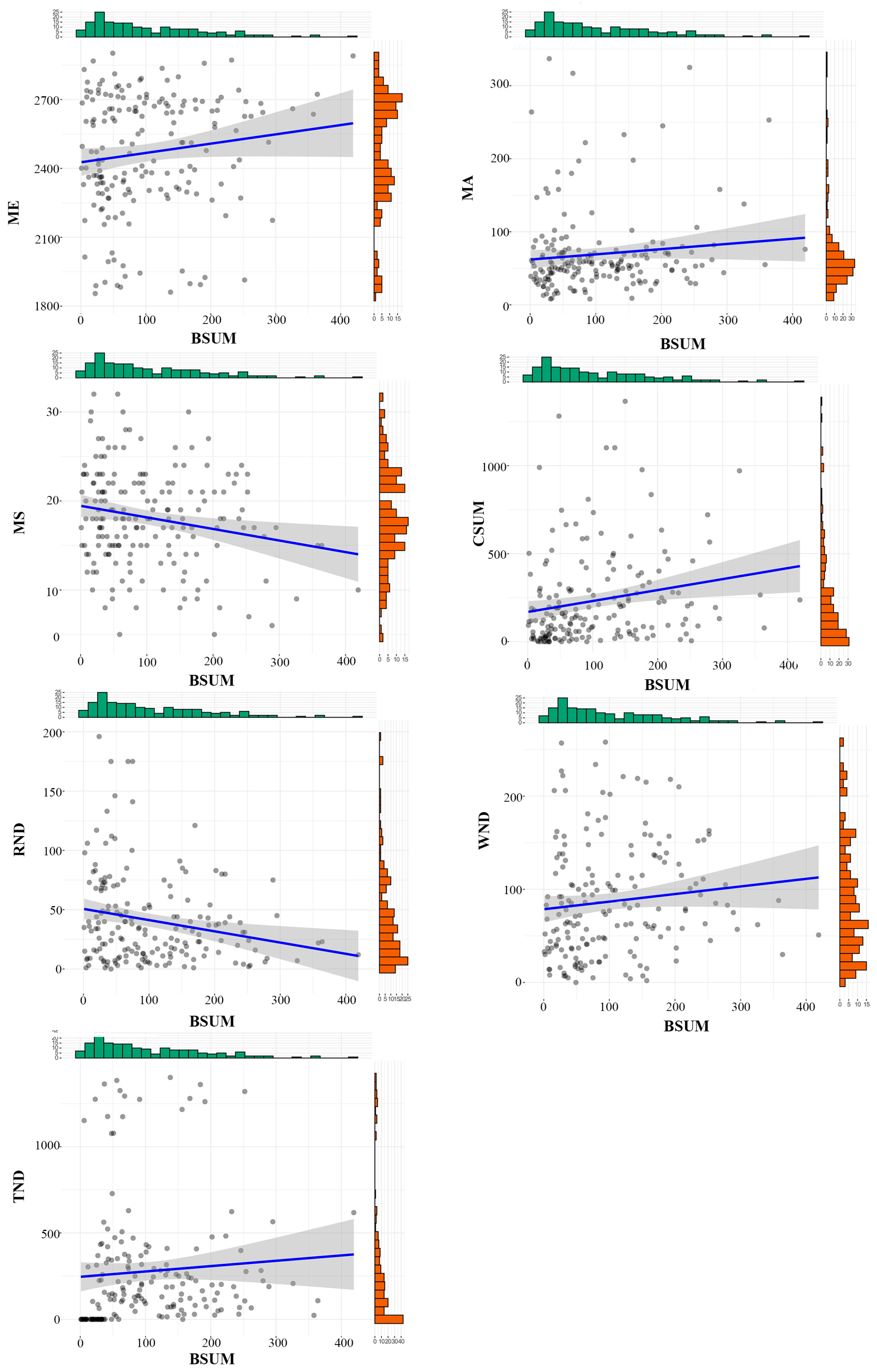
To illustrate the relationship between built-up area (BSUM) and the influencing factors, we created scatterplot matrix. BSUM shows positive associations with ME, MA, CSUM, WND, and TND, suggesting that larger built-up areas are generally found at higher altitudes, near farmland, and close to cultural landmarks and water sources. By contrast, BSUM is negatively associated with MS and RND, indicating that steep terrain and distance to major roads constrain the expansion of built-up land. These scatterplots highlight the heterogeneity of settlement distribution and different influencing factors (Figure 5).

3.2.1. Elevation and Settlement

Most settlements lie between 1890 m and 2902 m, with 38% of occupied cells clustered at 2600–2800 m. Another 27% fall at 2200–2400 m and 17% fall at 2400–2600 m, while only 8% sit below 2000 m and under 5% sit above 2800 m. Low areas face flood risk and make poor farmland; high elevations are too steep, cold, and thin-soiled. Thus, the 2600–2800 m zone—with its moderate slopes, mild climate, and good agricultural potential—is ideal for village development (Figure 6).

3.2.2. Slope and Settlement

About 75% of dense building cells sit on moderate slopes (15–30°), peaking around 20–25° where foundations are stable and terracing is easiest (mean = 23°, median = 22°). Steeper slopes over 30° see far fewer buildings because of landslide risk, soil instability, and infrastructure challenges. Very gentle slopes under 10° also have lower densities, likely because they lie near floodplains or suffer from poor drainage. In short, moderate slopes offer the best balance of stability, farming potential, and construction conditions for traditional settlements (Figure 6).

3.2.3. Aspect and Settlement

About 60% of dense settlements lie on east-to-southeast slopes (90–150°), which receive more sun and are sheltered from cold northwestern winds, improving both crop growth and living comfort. North-facing (315–360° and 0–45°) and west-facing (225–315°) slopes have far fewer buildings because they receive less sunlight and harsher, cooler winds. This pattern reflects traditional site choices aimed at maximizing warmth and agricultural productivity (Figure 6).

3.2.4. Road and Settlement

Most buildings sit within 10 m of paved village roads or provincial highways. From 10 to 50 m out, density drops to about 20%, where homes and farm buildings strike a balance between access and privacy. Beyond 50 m (up to 100 m), under 5% of buildings appear, scattered across fields and open land (Figure 6).

3.2.5. Water and Settlement

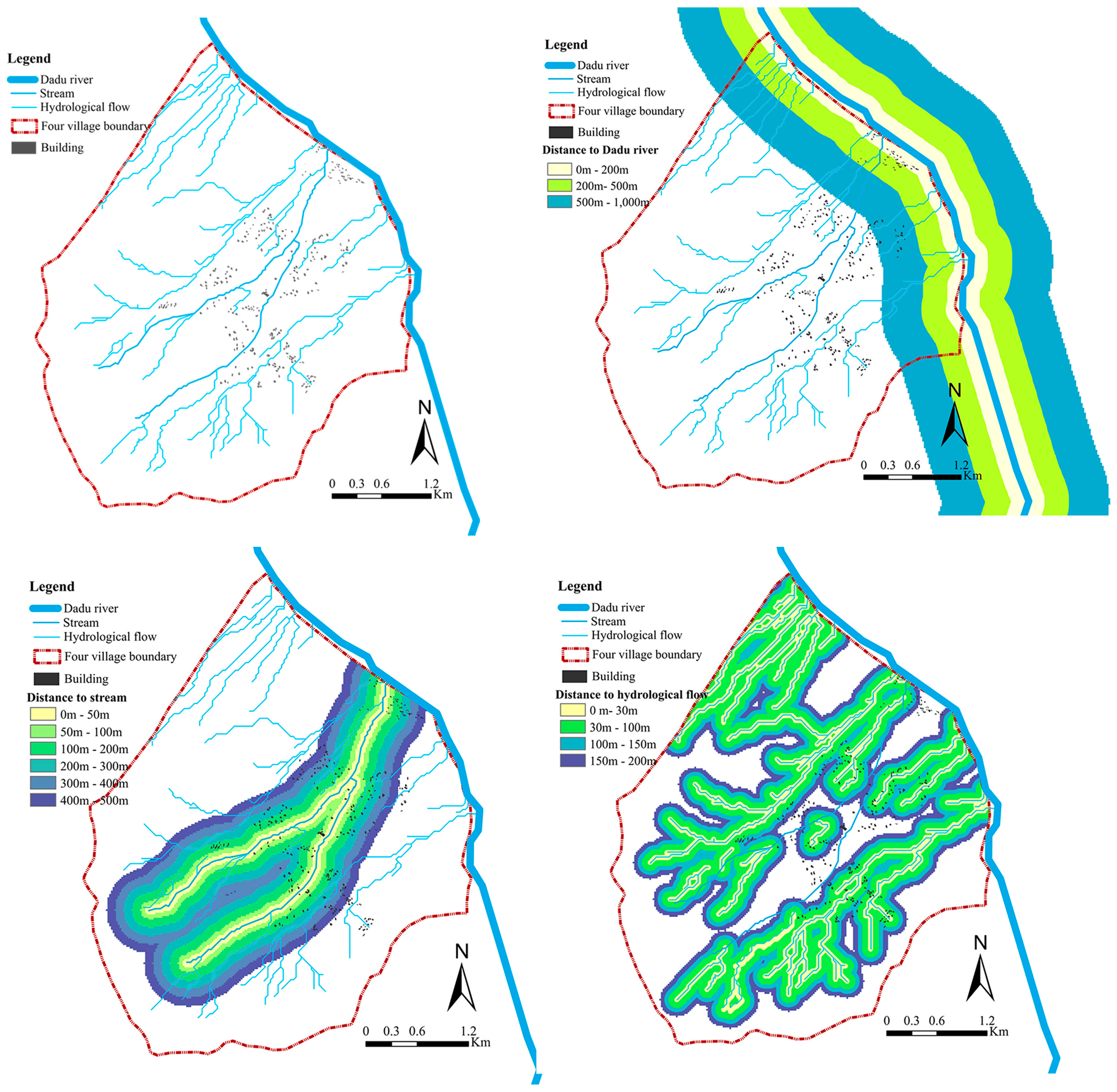
Settlements follow the water network’s tiers. Along the 80 m wide Dadu River, no homes sit within 100 m to prevent flooding; 14.3% lie 100–500 m away, and beyond 500 m, terraced fields and small villages fill the slopes. For two smaller streams, 82.5% of buildings stand 50–500 m back—keeping out of the 50 m flood buffer while ensuring easy irrigation. On the hills, most houses cluster within 200 m of runoff channels—set back about 30 m—to use natural drainage for irrigation, cut construction costs, and avoid landslide risk (Figure 7).

3.2.6. Towers and Settlement

The Euclidean distances between built-up grid cells and the nearest tower range from 0 m (indicating direct overlap) up to 1401.6 m. The mean distance is 278.1 m, while half of all cells lie within roughly 28.7 m (25th percentile) to 345.2 m (75th percentile) of a tower, and the median distance is 156.4 m. The large standard deviation (358.1 m) and long upper tail reflect a right-skewed distribution, with most building clusters concentrated within a few hundred meters of towers but a smaller number occurring over 1 km away.

3.3. Settlement Morphology

3.3.1. Global Moran’s I

The Global Moran’s I for the 100 × 100 m building–density grid is 0.3387 (expected under randomness = −0.0006). A z-score of 17.10 and p < 0.001 show that this clustering is highly significant, meaning dense and sparse areas form clusters rather than being randomly scattered. We used Euclidean distance with a 100 m threshold to define each neighborhood, and the low variance (0.000394) confirms that the pattern is not by chance. These findings reveal that settlement buildings cluster in response to factors like terrain, roads, and cropland.

3.3.2. Kernel Density Estimation (KDE)

The kernel density map highlights four main high-density cores (dark blue). The first is 100–300 m east of the main road on the Dadu River’s right bank at about 1900–2100 m of elevation; here, tightly packed, newer buildings suggest growth along the thoroughfare. In the southeast, two adjacent cores at 2600–2800 m sit on gentle slopes with broad farmland and older buildings—including historic towers—likely marking the original settlement. The fourth core in the northwest, around 2350 m, also lies on mild terrain but consists of more recent structures. Between these cores, secondary belts (light blue to yellow) about 200–300 m wide show density fading outward. In contrast, ridges above 2900 m and steep cliffs have almost no buildings, creating clear blank zones (Figure 8).

3.3.3. Convex Map

We used convex hulls to draw the smallest enclosing polygons for all settlement buildings (blue Settlement Hull) and all tower buildings (yellow Towers Hull) (Figure 9). The Settlement Hull wraps around every housing cluster on gentle terraces between about 2300 m and 2800 m of elevation. The Towers Hull cuts a concave shape around towers sitting at 2600–2700 m on subtle ridges, slicing inward by up to 150 m on the eastern slope to overlook both the village below and the upland approach. Where these hulls overlap—around the 2450 m–2940 m terrace—homes and towers intermingle, forming a compact core where daily life and defense work together. Outside this shared zone, the tower boundary pulls back toward the ridge crest, leaving some homes inside the Settlement Hull but beyond the towers’ reach. These patterns show how defensive geometry shaped the village’s form.

3.4. Regression Analysis

The dependent variable is built-up area (BSUM). Independent variables include the mean slope (MS), mean elevation (ME), mean aspect (MA), the distance to the nearest water (WND), the distance to the nearest road (RND), the distance to the nearest historic tower (TND), and cropland area (CSUM) (Table 2).

3.4.1. OLS

OLS regression explains about 36.4% of the variation in (BSUM (Multiple R2 = 0.364; Adjusted R2 = 0.362). MShas the strongest effect (|β| = 0.4269), followed by TND (|β| = 0.124) and CSUM (|β| = 0.0693). RND (|β| = 0.0128) and WND; |β| = 0.0088) have modest negative and positive effects, while (ME; (|β| = 0.0070) has the smallest impact. However, tests show the data are not normally distributed and residuals exhibit heteroskedasticity (Koenker BP p < 0.001). Despite low multicollinearity (all VIFs < 7.5), the modest adjusted R2 means that the global model captures only about a third of the observed variability. These results reveal spatial variation and local differences that one global model cannot capture. Geographically weighted regression (GWR) addresses this by allowing coefficients to vary by location, exposing place-specific effects—such as stronger slope constraints on ridge-top hamlets versus valleys, or different influences of farmland area and water distance in upland versus lowland villages. In short, heteroskedasticity, non-normal residuals, and weak global explanatory power all underscore the need for GWR to uncover the nuanced, localized drivers of village development.

3.4.2. GWR

The GWR model, using an adaptive bi-square bandwidth of 511 neighbors, fits the data much better than the global OLS. Its local R2 jumps to 0.5506 (adjusted R2 = 0.5328), the AICc drops by about 521 points to 16,865.85, and the residual sum of squares falls by 559,941 to 1,352,319. The error standard deviation shrinks to 28.20, and the cross-validation score improves from 1105.81 to 873.27. An ANOVA test confirms that these gains are highly significant (F ≈ 11.87, p ≪ 0.01), showing that allowing coefficients to vary by location captures important local variations in built-up density that the global model misses. Table 3 summarizes each predictor’s GWR statistics: Mean indicates the overall average effect; Std. Dev. captures spatial variability; Min/Max shows the range of local coefficient values; and % Sig (|t| ≥ 1.96) reports the proportion of grid cells where the effect is statistically significant at the 95% level, reflecting the factor’s widespread influence (Table 3).
  • Intercept
The GWR local intercept shows the baseline built-up area (BSUM) when all predictors are zero. Its mean is −1.85 (SD 47.90), ranging from −153.67 to +219.02, revealing large spatial variation in settlement density. Only 25.5% of grid cells have a significant intercept (|t| ≥ 1.96), meaning that in about three-quarters of the area, elevation, slope, road distance, and crop density together explain the built-up area. Positive intercept “hotspots” match terraced bench cores, while steep conservation zones along the gorge show significantly negative intercepts.
2.
Cropland Area (CSUM)
Cropland-area coefficients average at 0.0730 (SD 0.0652; range from −0.0005 to 0.2634) and are significant in 75% of cells. The strongest positive effects occur around village road peripheries—especially at main intersections and spur routes—where each unit of crop density greatly boosts settlement growth (up to +0.2634). In contrast, mid-slope settlement cores have coefficients near zero or that are slightly negative, showing that network centrality drives edge growth but has little effect in the village heart (Figure 10).
3.
Mean Elevation (ME)
The local elevation coefficient averages at 0.0072 (SD 0.0207; range from −0.0705 to 0.0800) and is significant in 60% of cells. It peaks on mid-slope terraces and gentle valley rims (up to +0.0800), where slight elevation gains provide stable ground, better drainage, and a mild microclimate. Ridge tops and steep uplands have coefficients near zero or down to −0.0705, reflecting harsher, exposed conditions. Thus, elevation aids building on moderate slopes but limits expansion in the highest, most exposed zones (Figure 10).
4.
Mean Aspect (MA)
Aspect coefficients average at 0.0035 (SD 0.0409; range from −0.0893 to 0.1442) and are significant in 40% of cells. The most positive effects appear on south- and southeast-facing slopes, which receive more sun and stay warmer, slightly boosting construction. North- and northeast-facing slopes show the strongest negative values, as cooler, shaded conditions restrict building (Figure 10).
5.
Mean Slope (MS)
Slope is the main physical limiter. The slope coefficient averages at −0.4046 (SD 0.4752; range form −2.1251 to 0.0018) and is significant in 70% of cells. Very steep areas (up to 35° near the gorge) have strong negative values, reflecting erosion risks and high infrastructure costs. Moderate slopes (10–20°) on terraces have coefficients near zero, showing little effect. This highlights slope gradient as a key barrier in steep relief but not on flat or gently rolling land (Figure 10).
6.
Distance to Water (WND)
The water-distance coefficient averages at 0.0279 (SD 0.0412; range from −0.0024 to 0.1960) and is significant in 50% of cells. It peaks on mid-slope terraces and plateau ridges (up to +0.1960), where moderate distance from main channels lowers flood risk while keeping water access. Valley bottoms and narrow riparian strips show coefficients that are near zero or slightly negative (down to −0.0024), since flood susceptibility and stream proximity limit building. This underscores that water access is essential but being too close to streams deters settlement (Figure 10).
7.
Distance to Road (RND)
The road-distance coefficient averages at −0.0226 (SD 0.0352; range from −0.1977 to 0.0241) and is significant in 48.9% of cells. The strongest negative effects (down to −0.1977) occur along valley bottoms and main transport corridors, showing that each extra meter from a road hinders development. Small positive effects (up to +0.0241) appear on upslope terraces and in the historic core, suggesting that some sites were set back from roads for defensive reasons (Figure 10).
8.
Towers Near Dist (TND)
The TND coefficient, which measures how proximity to defense towers affects built-up area, has a mean of 0.3130, a standard deviation of 0.2534, and ranges from 0.0489 to 1.6338. In 99% of grid cells, this effect is statistically significant (|t| ≥ 1.96), underscoring towers as focal points for settlement clustering. Near the village core—where towers historically provided protection and social order—each meter closer sharply increases building density, reflecting their protective and cultural draw. On the valley floor and at the settlement edges, however, this positive effect weakens, marking the outer limits of tower influence on where people build (Figure 10).

4. Discussion

4.1. Relationship Between Major Environmental Elements and Cultural Elements

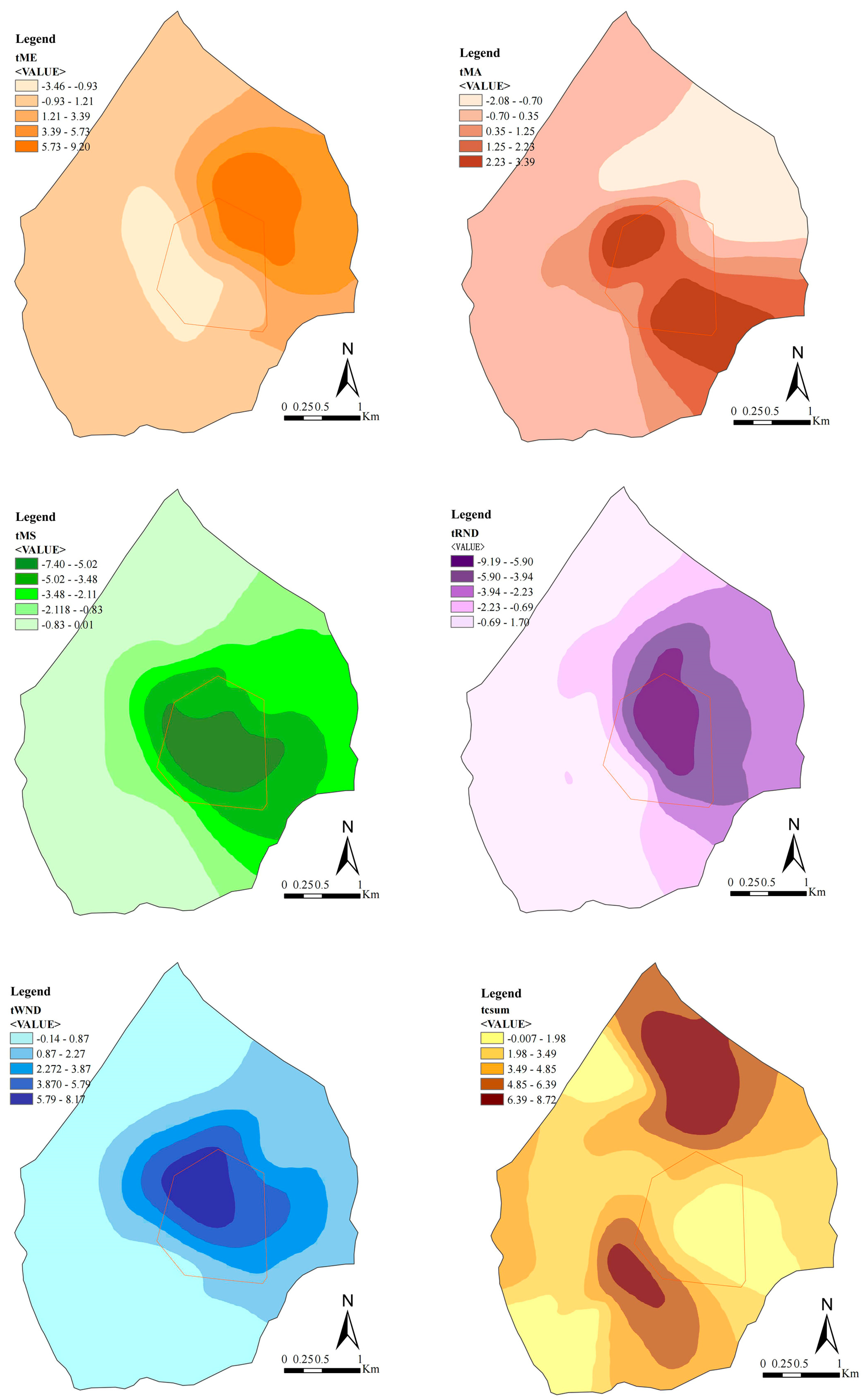
To explore how the culture and environment shaped building locations, we overlaid the tower heritage zone on maps of local regression t-values and found that all peaks lie within this area (Figure 9): the gentlest slopes (tMS = −7.40 to −5.02) cluster at the core, southeast-facing terraces (tMA = 2.23 to 3.39) sit just inside the boundary, the strongest water links (tWND = 5.79 to 8.17) and the most deliberate road setbacks (tRND = −9.19 to −5.90) fall within the wireframe, while farmland variation (tCSUM = 4.85 to 6.39) and elevation (tME) are uniformly distributed and thus do not explain building clusters. This overlap shows that Tibetans in Sopo Township, Damba County, balanced fertile land, manageable terrain, sunny exposures, water access, and transport links to form a compact settlement core. Lacking wider regional data, the tower zone likely marks the village’s original heart—a view confirmed by 2019 finds of Neolithic sites in Ze Chow village within that same polygon [49].

4.2. Strategies for Sustainable Development

4.2.1. Core Protected Zone

Based on the GWR analysis, the strongest positive influence on settlement density originates from proximity to the traditional stone tower clusters. Accordingly, the Core Protected Zone is suggested to encompass an area that is defined by the outer boundary of the tower cluster and surrounding traditional residences (approximately a 200-m radius) (Figure 11). Within this zone, new construction should be avoided, and any changes kept minimal to protect the traditional character [50]. Repairs are recommended to follow the original form, scale, and materials, with rooflines kept within about 1 m of the historic profile and building dimensions left unchanged. And restoration should use local stone, timber, and clay, as traditionally applied in Danba’s houses, while modern materials such as concrete or ceramic tile are best avoided [51]. The street grid, courtyards, and open spaces should remain intact, ensuring that the traditional layout and sightlines of the towers and houses are preserved.
Finally, in the Core Protected Zone, cultural activities should stay low-impact and temporary—such as walking tours, small displays, or seasonal festivals—while avoiding large events or heavy infrastructure. In Danba, this means favoring gentle experiences like craft demonstrations, traditional music, or village museums in existing courtyards. Such uses help preserve historic buildings and landscapes while allowing visitors to appreciate the living heritage.

4.2.2. Construction and Development Zone

Our research found that south- and southeast-facing slopes with gradients of 10–15°, situated within 100 m of roads and 50–100 m from streams, offer the best conditions for modest village expansion. These areas, which are just beyond the Core Protected Zone but still within service range, are called the Construction and Development Zone (Figure 11). New buildings here should follow the local building envelope formed by the three-to-four-story stone-and-timber dwellings that are common in the area. This ensures that expansion continues the traditional village form [52].
To improve the infrastructure in this area, three things will be done: minor road widening will be carried out through improvements to existing roadways, discreet drainage will use stone-lined swales and shallow subsurface drains that lead into vegetated trenches, and pedestrian paths will be laid out along natural contours. These methods, which have already been used in Tibetan villages like Jiaju in Danba, improve services while reducing ecological disturbance and maintaining cultural traditions [9]. Focusing on growth in these areas that have been shown to work allows villages to meet housing and service needs without damaging the landscape or sensitive environments. At the same time, improved housing and services in this zone can enhance well-being and education, helping to retain youth and sustain community vitality [53].

4.2.3. Ecological Conservation Zone

Our analysis shows that ecological risks arise both from steep slopes and from close proximity to rivers and streams. To address these issues, the Ecological Conservation Zone is subdivided into three complementary components. First, the Slope Stabilization Ecological Forest Zone encompasses slopes steeper than 25° and areas of original forest cover, where development is prohibited and restoration forestry is encouraged to reduce landslide and erosion risks [54,55] (Figure 11).
Second, Hydro-Ecological Corridors are designated along waterways, with no-build buffers of 50 m on main streams and 30 m on surface runoff channels, to protect riparian stability and mitigate soil and water loss (Figure 11). Within these corridors, measures such as planting poplars and willows to stabilize riverbanks, introducing nitrogen-fixing Sichuan alder, and reinforcing slopes with sea buckthorn or alpine meadow grasses are recommended [56,57]. Terraces should be maintained with dry-stone walls and vegetated staking, while contour drains and filter strips help manage runoff. Finally, the Ecological Rehabilitation Zone targets upper mountain areas that have been ecologically damaged, including sites of ruined towers, where habitat recovery, native species reintroduction, and cultural landscape rehabilitation are emphasized (Figure 11).
The Ecological Conservation Zone focuses on keeping the land healthy and making the village landscape stronger. These measures emphasize ecological safety as the foundation for long-term cultural and economic vitality.

4.2.4. Industry Development Zone

In the GWR analysis, cropland area (CSUM) showed a strong positive effect on the development of peripheral road network node settlements (β highest neighbor = 0.26, 75% of units significant), indicating strong potential for agri-tourism development where farmland and road access coincide (Figure 11). Chinese planning and land-use guidelines emphasize that tourism infrastructure in rural villages should remain a small, controlled fraction of land use. The central government action plan for rural tourism (2018–2020) instructs that township land-use plans may reserve at most 5% of their construction land quota for “scattered, single-site rural tourism facilities”. In Jiaju Village, for example, more than 98% of land remains farmland or forest, with only 1.5% used for tourism facilities. Based on this, orchards, tea gardens, and farm-experience areas can be developed at the edge of the Core Protected Zone, with the total scale kept within 5% of arable land, while supporting facilities (picking gardens, farmhouse restaurants) are best placed along main roads and linked by pedestrian paths. Industry development here should follow a community-led model. According to China Tourism News, Danba has developed a homestay alliance model with standardized criteria, unified management, and centralized marketing. This model has raised service quality and ensure more equitable benefit-sharing [58].
For long-term sustainability, the zone should apply carrying-capacity controls (visitor quotas, booking systems), require on-site wastewater treatment, and adopt permeable paving with vegetated buffers. These measures are consistent with the Ganzi Prefecture Rural Road Network Plan (2021–2035), which integrates boutique homestays and tourism into transport nodes, and the Sichuan Provincial 14th Five-Year Culture and Tourism Plan, which promotes “agriculture + tourism,” boutique rural stays, and seasonal festivals. Paired with cultural and environmental education, industry development can foster knowledge transfer, sustain traditions, and improve long-term quality of life [53].

4.3. Limitations and Challenges

While this study highlights the potential of micro-scale spatial–environmental analysis, several limitations remain. The work relied primarily on satellite imagery, digital elevation models, and limited field validation. These datasets enabled detailed modeling of environmental drivers but did not capture the humanistic and socio-economic dimensions of settlement development. Household structures, livelihood strategies, cultural practices, and governance arrangements were not systematically included, mainly due to time constraints in field surveys and the difficulty of obtaining consistent, fine-grained socio-economic data in remote areas. Consequently, the analysis emphasizes environmental influences while underrepresenting cultural and social processes.
In addition, high-resolution satellite imagery from World Imagery Wayback is available for the study area only after 2014. Since little land-use change occurred during this period, the study was restricted to a cross-sectional perspective and could not examine temporal dynamics.
Future research should address these gaps through comprehensive village-level surveys documenting livelihoods, cultural practices, and community perceptions. Incorporating such humanistic dimensions alongside spatial data would yield a more holistic understanding of settlement resilience and support planning strategies that reflect both ecological suitability and the lived realities of local communities.

5. Conclusions

This study employed a micro-scale spatial–environmental coupling framework, integrating land classification, settlement morphology, and geographically weighted regression (GWR) to investigate the drivers of traditional Tibetan village development in Suopo Township. The results demonstrate that settlement distribution is shaped by the combined influence of slope, elevation, aspect, proximity to roads and streams, cropland patterns, and the cultural presence of defensive towers. These findings were translated into four functional zoning strategies: Core Protection, Construction and Development, Ecological Conservation, and Industry Development. These strategies offer a practical framework for reconciling heritage preservation with sustainable growth.
Moreover, the methodology has broader applicability for master planning in mountainous heritage regions. By providing fine-grained spatial diagnostics, the framework enables planners to identify zones of ecological risk, cultural significance, and expansion suitability. This facilitates decision-making that is both evidence-based and culturally responsive, particularly in contexts where topographic constraints and heritage values must be balanced against modernization pressures. Applied at township or county scales, these micro-analyses can complement existing master plans by adding local specificity, thereby informing zoning regulations, infrastructure improvements, and tourism development strategies.
Several limitations must be acknowledged. The analysis relied primarily on environmental data and high-resolution imagery, with limited integration of socio-economic or cultural dimensions. As a result, factors such as household livelihoods, governance systems, and community aspirations remain underrepresented. In addition, the cross-sectional design, shaped by data availability, restricts the exploration of temporal dynamics in settlement evolution. Future research should therefore combine longitudinal imagery with village-level socio-cultural surveys to more fully capture both environmental adaptation and community agency.
Across international case studies, there are few examples where high-resolution environmental drivers are directly coupled with village-scale spatial morphology, or where such coupling frameworks are explicitly applied to specific village planning. This methodological emphasis highlights both the originality and the transferability of our approach. In conclusion, this research underscores the value of linking micro-scale spatial analysis with planning-oriented zoning strategies to safeguard cultural landscapes while supporting sustainable rural development. By integrating statistical modeling with practical planning tools, it offers a replicable pathway for balancing ecological integrity, cultural continuity, and rural revitalization in fragile mountain environments.

Author Contributions

Conceptualization, Z.L., W.H. and J.L.; methodology, Z.L.; software Z.L. and W.H.; validation, Z.L. and W.H.; formal analysis, Z.L. and W.H.; investigation, Z.L.; resources, Z.L. and W.H.; data curation, Z.L.; writing—original draft preparation, Z.L.; writing—review and editing, Z.L. and W.H.; visualization, Z.L. and W.H.; supervision, J.L.; project administration, J.L.; funding acquisition, J.L. All authors have read and agreed to the published version of the manuscript.

Funding

This research was funded by the Planning Fund Research Projects of Humanities and Social Sciences of the Ministry of Education (Grant No. 24XJA760003).

Institutional Review Board Statement

Not applicable.

Informed Consent Statement

Not applicable.

Data Availability Statement

The data presented in this study are available from the corresponding author upon reasonable request.

Acknowledgments

We thank the other professors and students of the Vernacular Architecture Research Team for their support. We also extend our gratitude to the Editor and each reviewer for their patience and valuable feedback, which greatly contributed to the improvement of this study.

Conflicts of Interest

The authors declare no conflicts of interest.

References

  1. Klein, J.A.; Tucker, C.M.; Nolin, A.W.; Hopping, K.A.; Reid, R.S.; Steger, C.; Grêt-Regamey, A.; Lavorel, S.; Müller, B.; Yeh, E.T.; et al. Catalyzing Transformations to Sustainability in the World’s Mountains. Earths Future 2019, 7, 547–557. [Google Scholar] [CrossRef]
  2. Yang, E.; Yao, Q.; Long, B.; An, N.; Liu, Y. Progress in the Research of Features and Characteristics of Mountainous Rural Settlements: Distribution, Issues, and Trends. Sustainability 2024, 16, 4410. [Google Scholar] [CrossRef]
  3. Xi, C.; Qian, T.; Chi, Y.; Chen, J.; Wang, J. Relationship between Settlements and Topographical Factors: An Example from Sichuan Province, China. J. Mt. Sci. 2018, 15, 2043–2054. [Google Scholar] [CrossRef]
  4. Xu, J.; Li, Z.; Ma, R.; Han, T. Correlation between Distribution of Rural Settlements and Topography in Plateau-Mountain Area: A Study of Yunnan Province, China. Sustainability 2023, 15, 3458. [Google Scholar] [CrossRef]
  5. Wu, C.; Yang, M.; Wei, H.; Gong, L.; Tan, G. Spatial Variability of Cultural Landscape Vulnerability and Influential Factors in Ethnic Villages of Southeast Guizhou. Sci. Rep. 2025, 15, 1491. [Google Scholar] [CrossRef]
  6. Fan, D.; Maliki, N.Z.B.; He, C.; Bi, Y.; Yu, S. Cultural Gene Characterization and Mapping of Traditional Tibetan Village Landscapes in Western Sichuan, China. npj Herit. Sci. 2025, 13, 317. [Google Scholar] [CrossRef]
  7. Li, J.H.; Liu, N. Ecological Wisdom and Renewal of Jiarong Tibetan Residence in Zhonglu West Sichuan Province. Adv. Mater. Res. 2012, 450–451, 1493–1497. [Google Scholar] [CrossRef]
  8. Assessment of Resilience and Key Drivers of Tibetan Villages in Western Sichuan—PMC. Available online: https://pmc.ncbi.nlm.nih.gov/articles/PMC12214665/ (accessed on 20 July 2025).
  9. Meng, Q.; Wang, C.; Xu, T.; Pi, H.; Wei, Y. Evaluation of the Sustainable Development of Traditional Ethnic Village Tourist Destinations: A Case Study of Jiaju Tibetan Village in Danba County, China. Land 2022, 11, 1008. [Google Scholar] [CrossRef]
  10. Li, Y.; Fan, W.; Yuan, X.; Li, J. Spatial Distribution Characteristics and Influencing Factors of Traditional Villages Based on Geodetector: Jiarong Tibetan in Western Sichuan, China. Sci. Rep. 2024, 14, 11700. [Google Scholar] [CrossRef] [PubMed]
  11. Fan, D.; Maliki, N.Z.B.; Yu, S. Fractal Characteristics and Influencing Factors of Landscape Space of Tibetan Rural in Western Sichuan: A Case Study of Three Traditional Villages. Front. Urban Rural Plan. 2023, 1, 22. [Google Scholar] [CrossRef]
  12. Shen, W.; Chen, Y.; Rong, P.; Li, J.; Yan, W.; Cheng, J. The Spatial Coupling and Its Influencing Mechanism between Rural Human-Habitat Heritage and Key Rural Tourism Villages in China. npj Herit. Sci. 2025, 13, 79. [Google Scholar] [CrossRef]
  13. Hua, H.; Zhou, S. Human-Environment System Boundaries: A Case Study of the Honghe Hani Rice Terraces as a World Heritage Cultural Landscape. Sustainability 2015, 7, 10733–10755. [Google Scholar] [CrossRef]
  14. Zhang, Y.; He, Y. Human-Land Relationship in the Construction of Historical Settlements Based on Complex Adaptive System (CAS) Theory: Evidence from Shawan in Guangfu Region, China. Herit. Sci. 2024, 12, 173. [Google Scholar] [CrossRef]
  15. Oikonomopoulou, E.; Delegou, E.T.; Sayas, J.; Vythoulka, A.; Moropoulou, A. Preservation of Cultural Landscape as a Tool for the Sustainable Development of Rural Areas: The Case of Mani Peninsula in Greece. Land 2023, 12, 1579. [Google Scholar] [CrossRef]
  16. Liu, Y.; Liu, Y.; Deng, W.; Deng, W.; Song, X.; Song, X. Relief Degree of Land Surface and Population Distribution of Mountainous Areas in China. J. Mt. Sci. 2015, 12, 518–532. [Google Scholar] [CrossRef]
  17. Li, X.; Li, H.; Zhang, Y.; Yang, L. Spatial Patterns and the Regional Differences of Rural Settlements in Jilin Province, China. Sustainability 2017, 9, 2170. [Google Scholar] [CrossRef]
  18. Ma, L.; Guo, X.; Tian, Y.; Wang, Y.; Chen, M. Micro-Study of the Evolution of Rural Settlement Patterns and Their Spatial Association with Water and Land Resources: A Case Study of Shandan County, China. Sustainability 2017, 9, 2277. [Google Scholar] [CrossRef]
  19. Liu, Y.; Deng, W.; Peng, L. The Coupling Mechanism between the Suitable Space and Rural Settlements Considering the Effect of Mountain Hazards in the Upper Minjiang River Basin. J. Mt. Sci. 2020, 17, 2774–2783. [Google Scholar] [CrossRef]
  20. Zhang, Y.; Wang, Z.; Hu, S.; Song, Z.; Cui, X.; Afriyie, D. Spatial and Temporal Evolution and Prediction of the Coordination Level of “Production-Living-Ecological” Function Coupling in the Yellow River Basin, China. Int. J. Environ. Res. Public Health 2022, 19, 14530. [Google Scholar] [CrossRef]
  21. Yao, L.; Li, X.; Li, Q.; Wang, J. Temporal and Spatial Changes in Coupling and Coordinating Degree of New Urbanization and Ecological-Environmental Stress in China. Sustainability 2019, 11, 1171. [Google Scholar] [CrossRef]
  22. Zheng, W.; Cao, W.; Li, G.; Zhu, S.; Zhang, X. Spatial Pattern Characteristics and Factors for the Present Status of Rural Settlements in the Lijiang River Basin Based on ArcGIS. Int. J. Environ. Res. Public Heal. 2023, 20, 4124. [Google Scholar] [CrossRef]
  23. Peng, Y.; Qiu, H.; Wang, X. The Influence of Spatial Functions on the Public Space System of Traditional Settlements. Sustainability 2023, 15, 8632. [Google Scholar] [CrossRef]
  24. Liu, Y.; Ke, X.; Wu, W.; Zhang, M.; Fu, X.; Li, J.; Jiang, J.; He, Y.; Zhou, C.; Li, W.; et al. Geospatial Characterization of Rural Settlements and Potential Targets for Revitalization by Geoinformation Technology. Sci. Rep. 2022, 12, 8399. [Google Scholar] [CrossRef] [PubMed]
  25. Zhang, Y.; Wang, P.; Wang, T.; Cai, C.; Li, Z.; Teng, M. Scenarios Simulation of Spatio-Temporal Land Use Changes for Exploring Sustainable Management Strategies. Sustainability 2018, 10, 1013. [Google Scholar] [CrossRef]
  26. Tao, G.; Li, X.; Tian, S.; Li, H.; Song, Y. Influence of Human Settlements Factors on the Spatial Distribution Patterns of Traditional Villages in Liaoning Province. Humanit. Soc. Sci. Commun. 2024, 11, 1757. [Google Scholar] [CrossRef]
  27. Zhou, X.; Wang, Z.; Liu, Y.; Cheng, Y.; Zhou, Y.; Zhang, J. Factors Influencing the Evolution of Rural Settlements Based on MGWR: A Case Study of Haikou City. Trop. Geogr. 2023, 43, 1599–1610. [Google Scholar] [CrossRef]
  28. Chen, S.; Mehmood, M.S.; Liu, S.; Gao, Y. Spatial Pattern and Influencing Factors of Rural Settlements in Qinba Mountains, Shaanxi Province, China. Sustainability 2022, 14, 10095. [Google Scholar] [CrossRef]
  29. Yang, Z.; Yang, D.; Geng, J.; Tian, F. Evaluation of Suitability and Spatial Distribution of Rural Settlements in the Karst Mountainous Area of China. Land 2022, 11, 2101. [Google Scholar] [CrossRef]
  30. Li, K.; Geng, H.; Yue, L.; Li, K.; Huang, L. Spatial Differentiation Characteristics and Driving Mechanism of Rural Settlements Transformation in the Metropolis: A Case Study of Pudong District, Shanghai. Front. Environ. Sci. 2021, 9, 755207. [Google Scholar] [CrossRef]
  31. Yang, X.; Pu, F. Spatial Cognitive Modeling of the Site Selection for Traditional Rural Settlements: A Case Study of Kengzi Village, Southern China. J. Urban Plan. Dev. 2020, 146, 05020026. [Google Scholar] [CrossRef]
  32. Zhang, R.; Zhang, X. Distribution Characteristics and Influencing Factors of Rural Settlements in Metropolitan Fringe Area: A Case Study of Nanjing, China. Land 2022, 11, 1989. [Google Scholar] [CrossRef]
  33. You, T.; Yan, S. Spatial Differentiation and Driving Force Detection of Rural Settlements in the Yangtze River Delta Region. Sustainability 2023, 15, 8774. [Google Scholar] [CrossRef]
  34. Wang, J.; Wang, X.; Du, G.; Zhang, H. Temporal and Spatial Changes of Rural Settlements and Their Influencing Factors in Northeast China from 2000 to 2020. Land 2022, 11, 1640. [Google Scholar] [CrossRef]
  35. Yin, J.; Li, H.; Wang, D.; Liu, S. Optimization of Rural Settlement Distributions Based on the Ecological Security Pattern: A Case Study of Da’an City in Jilin Province of China. Chin. Geogr. Sci. 2020, 30, 824–838. [Google Scholar] [CrossRef]
  36. Rao, Y.; Zou, Y.; Chen, Y.; Feng, L.; Song, Y.; Wu, P.-L. Optimization of Rural Settlements Based on Rural Revitalization Elements and Rural Residents’ Social Mobility: A Case Study of a Township in Western China. Habitat Int. 2023, 137, 102851. [Google Scholar] [CrossRef]
  37. Fan, X.; Luo, W.; Yu, H.; Rong, Y.; Gu, X.; Zheng, Y.; Ou, S.; Tiando, D.S.; Zhang, Q.; Tang, G.; et al. Landscape Evolution and Simulation of Rural Settlements around Wetland Park Based on MCCA Model and Landscape Theory: A Case Study of Chaohu Peninsula, China. Int. J. Environ. Res. Public Health 2021, 18, 13285. [Google Scholar] [CrossRef]
  38. Qin, Y.; Luo, G.; Li, Y.; Tan, Q.; Zheng, C.; Yu, M.; Liao, J.; Li, M. Assessment of Sustainable Development of Rural Settlements in Mountainous Areas: A Case Study of the Miaoling Mountains in Southwestern China. Land 2022, 11, 1666. [Google Scholar] [CrossRef]
  39. Jia, A.; Yun, X.; Zheng, X.; Wen, X.; Liang, X.; Yun, Y. Towards Sustainable Rural Revitalization: A Multidimensional Evaluation of Rural Vitality in China’s Traditional Villages. Sustainability 2024, 16, 5408. [Google Scholar] [CrossRef]
  40. Liu, X.; Zhang, Y.; Li, Y.; Zhang, A.; Li, C. Exploring Village Spatial Patterns for Sustainable Development: A Case Study of Diqing Prefecture. Sustainability 2023, 15, 16362. [Google Scholar] [CrossRef]
  41. Zeybek, O.; Erdoğan, E. Transforming Traditional Villages into Sustainable Communities: Evaluating Ecovillage Potential in Bursa, Turkey. Sustainability 2025, 17, 2095. [Google Scholar] [CrossRef]
  42. Assen, Y.M.; Kura, A.L.; Dube, E.E.; Mensuro, G.K.; Debelo, A.R.; Gure, L.B. Climate Change Threats to UNESCO-Designated World Heritage Sites: Empirical Evidence from Konso Cultural Landscape, Ethiopia. Sustainability 2024, 16, 8442. [Google Scholar] [CrossRef]
  43. Stotten, R.; Schermer, M.; Wilson, G.A. Lock-ins and Community Resilience: Two Contrasting Development Pathways in the Austrian Alps. J. Rural. Stud. 2021, 84, 124–133. [Google Scholar] [CrossRef]
  44. Chaudhary, S.; Wang, Y.; Dixit, A.M.; Khanal, N.R.; Xu, P.; Yan, K.; Liu, Q.; Lu, Y.; Li, M. Eco-Environmental Risk Evaluation for Land Use Planning in Areas of Potential Farmland Abandonment in the High Mountains of Nepal Himalayas. Sustainability 2019, 11, 6931. [Google Scholar] [CrossRef]
  45. Zeballos-Velarde, C.; Córdova, M.; Bronfman, N.C. The Role of Ancestral Practices as Social Capital to Enhance Community Disaster Resilience: The Case of the Colca Valley, Peru. Int. J. Disaster Risk Reduct. 2023, 92, 103737. [Google Scholar] [CrossRef]
  46. Belgiu, M.; Drăguţ, L. Random Forest in Remote Sensing: A Review of Applications and Future Directions. ISPRS J. Photogramm. Remote Sens. 2016, 114, 24–31. [Google Scholar] [CrossRef]
  47. Dong, L.; Du, H.; Mao, F.; Han, N.; Li, X.; Zhou, G.; Zhu, D.; Zheng, J.; Zhang, M.; Xing, L.; et al. Very High Resolution Remote Sensing Imagery Classification Using a Fusion of Random Forest and Deep Learning Technique—Subtropical Area for Example. IEEE J. Sel. Top. Appl. Earth Obs. Remote Sens. 2020, 13, 113–128. [Google Scholar] [CrossRef]
  48. Gao, Y.; Zhao, J.; Han, L. Exploring the Spatial Heterogeneity of Urban Heat Island Effect and Its Relationship to Block Morphology with the Geographically Weighted Regression Model. Sustain. Cities Soc. 2022, 76, 103431. [Google Scholar] [CrossRef]
  49. Liu, H.; Li, W. Archaeological Investigation on the Remains of the Pre-Qin and Han Dynasties in Danba County, Ganzi Tibetan Autonomous Prefecture, Sichuan Province. J. Xizang Minzu Univ. (Philos. Soc. Sci. Ed.) 2022, 43, 68–81. [Google Scholar]
  50. Li, J.; Lin, F.; Yang, S.; Chen, Y. Spatial Planning Strategies for Urban Ecology and Heritage Conservation in Macau: An Investigation of Ultra-High-Density Cities. Information 2024, 15, 799. [Google Scholar] [CrossRef]
  51. Xie, K.; Zhang, Y.; Han, W. Architectural Heritage Preservation for Rural Revitalization: Typical Case of Traditional Village Retrofitting in China. Sustainability 2024, 16, 681. [Google Scholar] [CrossRef]
  52. Feng, X.; Hu, M.; Somenahalli, S.; Zhang, W.; Liu, K.; Li, M.; Zhou, Z.; Li, F. Study on the Spatial Morphology of Ando Tibetan Traditional Villages in China: A Case of Traditional Villages in Huangnan Prefecture. Sustainability 2025, 17, 1353. [Google Scholar] [CrossRef]
  53. Korcz, N.; Kamińska, A.; Ciesielski, M. Is the Level of Quality of Life Related to the Frequency of Visits to Natural Areas? Forests 2024, 15, 2257. [Google Scholar] [CrossRef]
  54. Huang, H.; Ju, S.; Duan, W.; Jiang, D.; Gao, Z.; Liu, H. Landslide Monitoring along the Dadu River in Sichuan Based on Sentinel-1 Multi-Temporal InSAR. Sensors 2023, 23, 3383. [Google Scholar] [CrossRef]
  55. Ju, L.; Liu, Y.; Yang, J.; Xiang, M.; Xiang, Q.; Hu, W.; Ding, Z. Construction of Nature Reserves’ Ecological Security Pattern Based on Landscape Ecological Risk Assessment: A Case Study of Garze Tibetan Autonomous Prefecture, China. Sustainability 2023, 15, 8707. [Google Scholar] [CrossRef]
  56. Wan, X.; Zhang, F. An overview of Populus genetic resources in southwest China. For. Chron. 2013, 89, 79–87. [Google Scholar] [CrossRef]
  57. Zheng, Y.; Feng, M.; Li, X.; Huang, X.; Chen, G.; Bai, W.; Xu, X.; Li, J.; Li, X.; Leng, B.; et al. Phenotypic Variation Analysis and Excellent Clone Selection of Alnus cremastogyne from Different Provenances. Plants 2023, 12, 3259. [Google Scholar] [CrossRef]
  58. Shui, W.; Zhang, Y.; Wang, X.; Liu, Y.; Wang, Q.; Duan, F.; Wu, C.; Shui, W. Does Tibetan Household Livelihood Capital Enhance Tourism Participation Sustainability? Evidence from China’s Jiaju Tibetan Village. Int. J. Environ. Res. Public Health 2022, 19, 9183. [Google Scholar] [CrossRef]
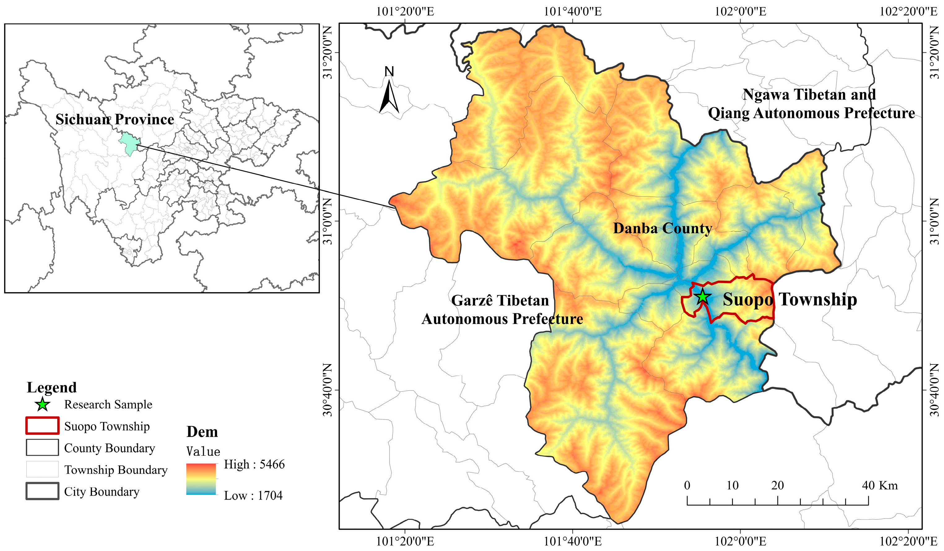
Figure 1. Geographical location of research area.
Sustainability 17 08766 g001
Figure 2. Four-step framework of this study.
Sustainability 17 08766 g002
Figure 3. Extraction of high-resolution imagery and land classification in the study area. (a) RF land classification of sample villages; (b) Google high-definition imagery of sample villages.
Sustainability 17 08766 g003
Figure 4. Land classification of four villages in Suopo township after post processing.
Sustainability 17 08766 g004
Figure 5. Scatterplots show that the relationship between built-up area (BSUM) and multiple influencing factors, including topographic features (mean elevation, ME; mean aspect, MA; mean slope, MS), cropland area (CSUM), and accessibility variables (distance to nearest road, RND; distance to nearest water body, WND; and distance to nearest historic tower, TND). Each panel displays the distribution of BSUM against one variable, with a fitted regression line (blue) and 95% confidence interval (shaded area).
Sustainability 17 08766 g005
Figure 6. Spatial distribution of topographic (elevation/aspect/slope) and road accessibility for buildings in the study area.
Sustainability 17 08766 g006
Figure 7. Proximity to the three-tier water network: Dadu river, streams, and runoff channels.
Sustainability 17 08766 g007
Figure 8. Kernel density analysis of sample settlements.
Sustainability 17 08766 g008
Figure 9. Minimal geometric boundaries for settlements and watchtowers.
Sustainability 17 08766 g009
Figure 10. Spatial Distribution of Local t-Values from GWR Analysis for Six Explanatory Variables.
Sustainability 17 08766 g010
Figure 11. Zoning strategies for sustainable development in the study area.
Sustainability 17 08766 g011
Table 1. Data sources.
DatasetSpatial/Temporal ResolutionPlatformPurpose
World Imagery (Esri)0.5–1 m, 2022–2023Global Mapper APITraining ROIs and Random Forest land-cover classification
SRTM DEM30 mhttps://www.gscloud.cnDerivation of slope, aspect and topographic position index (TPI)
OpenStreetMap (OSM)Vector, 2023 snapshotGeofabrikRoad network and settlement centroids
Hydrological network1:50,000 vectorNational HydroDatabaseDistance-to-water calculations
Field GPS points and high-res UAV photos<5 cmAuthor’s survey, 2022/10Independent validation samples (n = 200)
Table 2. Descriptive statistics of variables used in the OLS and GWR models.
TypeVariable (Code)Description (Unit)
DependentBSUMBuilt-up area per grid cell (m2)
IndependentMSMean slope of cell (°)
MEMean elevation of cell (m)
MAMean aspect of cell (°)
WNDDistance to nearest water body (m)
RNDDistance to nearest road (m)
TNDDistance to nearest historic tower (m)
CSUMCropland area per grid cell (m2)
Table 3. Summary statistics of GWR local coefficient estimates and percentage of significant coefficients.
VariableMeanStd. Dev.MinMax% Sig (|t| ≥ 1.96)
Intercept−1.801447.8503−153.672219.01925.5%
CSUM0.07300.0652−0.00050.263475%
ME0.00720.0207−0.07050.080060%
MA0.00350.0409−0.08930.144240%
MS−0.40460.4752−2.12510.001870%
WND0.02790.0412−0.00240.196050.0%
RND−0.02260.0352−0.19770.024148.9%
TND0.31300.25340.04891.633899%
Disclaimer/Publisher’s Note: The statements, opinions and data contained in all publications are solely those of the individual author(s) and contributor(s) and not of MDPI and/or the editor(s). MDPI and/or the editor(s) disclaim responsibility for any injury to people or property resulting from any ideas, methods, instructions or products referred to in the content.