1. Introduction
Accurate forecasting of national energy demand is critical for maintaining grid stability, managing supply chains, and supporting essential infrastructure and economic planning. In The Netherlands, rising grid congestion, increased dependence on renewable energy, and heightened climate and economic variability have made long-term forecasting more challenging [
1,
2].
To improve energy grid management, more accurate predictions of future Dutch energy consumption are required. One proposed solution is real-time load forecasting and demand response in smart grids [
3]. This solution depends heavily on the precision of forecasting models.
Traditional forecasting models often rely on statistical methods or deep learning, but both approaches have limitations when applied in isolation. Ensemble methods, such as Prophet–LSTM, have shown promise by combining interpretable trend and seasonality modelling with deep temporal feature extraction [
4]. Recent work in quantum machine learning (QML) indicates that quantum-enhanced neural networks can model high-dimensional temporal dependencies more efficiently [
5,
6,
7].
However, existing research has not yet explored the integration of ensemble methods like Prophet with quantum-enhanced architectures such as Quantum Long Short-Term Memory (QLSTM) networks. Furthermore, macroeconomic variables have not been systematically combined with climate predictors despite evidence that these indicators, such as GDP and commodity futures, are critical drivers of long-term energy use [
8,
9]. Taken together, the absence of (i) an integrated Prophet–QLSTM pipeline and (ii) a joint climate–macroeconomic predictor set for national, long-horizon demand forecasting constitutes the central research gap addressed in this paper.
This study investigates whether a hybrid quantum–classical forecasting pipeline, combining the Prophet framework with a Quantum Long Short-Term Memory (QLSTM) model and enriched with both climate and economic predictors, can improve long-horizon energy demand forecasting in The Netherlands. This study evaluates four models: Prophet–LSTM and Prophet–QLSTM, with and without stacked generalisation, utilising Bayesian optimisation for feature selection and rolling-origin cross-validation for evaluation.
By bridging ensemble forecasting, quantum-enhanced architectures, and cross-domain feature integration, this work contributes a novel modelling approach to the field of energy forecasting. The results may provide practical value for infrastructure operators and policymakers seeking to anticipate future demand under increasing climate and economic uncertainty.
Accordingly, we pursue four objectives that mirror the research questions without presenting them as a list: (i) assess the year-round forecasting accuracy of a Prophet–QLSTM pipeline for national energy demand; (ii) quantify the added value of quantum-inspired components relative to a classical Prophet–LSTM baseline; (iii) determine which climate and macroeconomic predictors are most informative under Bayesian-guided feature selection; and (iv) analyse the trade-offs between hybrid quantum and classical machine-learning models, including accuracy, robustness, and implementation considerations under stacked and non-stacked settings.
Importantly, while the empirical analysis centres on The Netherlands, the modelling pipeline and evaluation protocol are general and can be ported to other national systems without loss of methodological validity. This article is organised as follows:
Section 2 reviews climate and macroeconomic predictors alongside hybrid quantum–classical forecasting approaches;
Section 3 details data sources, preprocessing, model architectures, and evaluation design;
Section 4 reports forecasting accuracy and ablation results;
Section 5 discusses practical implications, interdependencies, and limitations;
Section 6 concludes and outlines directions for future work.
From a sustainability perspective, more accurate long-horizon forecasts directly support renewable-integration targets, resource-adequacy assessments, and resilient grid operations under climate and economic uncertainty.
2. Literature Review
Forecasting national energy demand has been approached through four strands that motivate our design choices. First, decomposable statistical models such as Prophet capture trend, seasonality, and calendar effects in long spans of load data [
10]. Second, deep-learning approaches within smart-grid and residential contexts have shown that nonlinear temporal dependencies and multivariate exogenous inputs can materially improve accuracy when data are rich [
3,
11,
12]. Third, hybrid pipelines that combine decomposition with recurrent networks (e.g., Prophet–LSTM) report gains at the national scale by letting the statistical component explain low-frequency structure while the neural component models residual dynamics [
4]. Fourth, recent studies explore hybrid quantum–classical time-series models in energy and climate applications, indicating potential benefits from quantum-enhanced representations under certain regimes [
7,
13,
14]. Against this backdrop, we evaluate a Prophet–(Q)LSTM ensemble enriched with climate and macroeconomic predictors and compare it directly to its classical Prophet–LSTM counterpart, highlighting that—unlike prior work—we (i) integrate Prophet with a QLSTM core and (ii) jointly include climate and macroeconomic drivers for national, long-horizon demand forecasting.
2.1. Climate Predictors
The Dutch energy grid has become more volatile due to the dependence on green energy and recent climate variability [
15]. Therefore, climate features are a logical starting point for energy demand forecasting (EDF). We consider both large-scale climate signals that shape regional weather regimes and local observations for immediate demand drivers.
North Atlantic Oscillation (NAO). The NAO is regarded as a principal driver of climate variability in Europe, describing atmospheric circulation variability over the North Atlantic. It modulates the large-scale pressure field and thus weather over Western Europe, including The Netherlands [
15]. The NAO is linked to oceanic processes discussed below.
Sea surface temperature (SST/NAT). SST anomalies in the North Atlantic arise from atmosphere–ocean heat-flux variability and often exhibit a tripolar pattern (North Atlantic Temperature, NAT) closely associated with the NAO [
16].
Sea ice concentration (SIC). SIC influences ocean circulation and climate; although it covers about 7% of Earth’s surface, its variability partly drives broader circulation patterns [
17].
Local weather. To capture short-run load sensitivity, we use local weather observations (daily/hourly temperature, precipitation, wind) [
18].
The North Atlantic Oscillation (NAO), North Atlantic Tripole (NAT), and Sea Ice Concentration (SIC) provide slowly varying background variability, whereas local weather captures day-to-day variation in demand; both are included as exogenous regressors in our model.
More broadly, characterising the correlation structure among many exogenous drivers is a common approach in complex multivariate systems; our use of Pearson heatmaps for grouping/pruning highly collinear features is methodologically aligned with correlation–network analyses reported in other domains [
19].
2.2. Economic Predictors
In addition to climate data, research also points to economic data as an indicator of how much energy a country will consume, since macroeconomic trends and consumer behaviour influence energy consumption [
8].
Gross Products (GDP, GNP). Gross Domestic Product (GDP) is the first economic predictor for The Netherlands [
12]. GDP provides a measure of domestic economic productivity. The second dataset regards the Gross National Product (GNP). GNP accounts for international financial factors, making it an important complementary indicator of economic activity. It accounts for total national income, including international investments and remittances, which can further influence national energy consumption patterns [
20].
Inflation rate. Inflation rate is another economic predictor for The Netherlands. Inflation plays a large role in economic stability, which, according to Banna et al. [
2], is also a large factor in energy security risk (ESR) and therefore a feature that could be of interest when performing EDF.
Residential sector. Another economic factor considered is the residential sector, which significantly contributes to total energy consumption [
9,
11].
Labour participation. Labour-participation rate is also included, as reduced workforce participation can lead to shifts in economic productivity, which in turn influences GDP and GNP.
Energy prices and futures. Finally, global economic features are represented by energy prices and energy-commodity futures. Commodity futures are significant predictors for energy prices [
21]. Therefore, the energy prices and their subsequent future prices could be predictors worth looking into, since the energy prices themselves have been proven to be significant predictors [
4].
Related work in finance shows that forward-looking signals such as analyst forecasts can carry distinct predictive value; analogously, we include energy-commodity futures as expectations-oriented covariates in our forecasting setup [
22].
2.3. Quantum Computing
Quantum computing exploits the laws of quantum mechanics, which allow quantum states to exhibit atypical statistical patterns. These resources can generate correlations by using superposition and entanglement that classical systems cannot efficiently reproduce. Recent theoretical analyses and small-scale demonstrations suggest that such patterns can both generate and identify highly statistically complex data distributions. If this ability of recognising statistically complex patterns can be harnessed in quantum algorithms, there is potential to outperform their classical counterparts; this is known as
quantum speedup. The speedup would theoretically lead to the reduction of
query complexity, or in other words, would reduce the number of queries to the information source [
6]. But because large-scale fault-tolerant devices are not yet available, current research explores hybrid quantum–classical computing, in which noisy, intermediate-scale quantum processors are combined with classical optimisers to test these ideas experimentally [
23].
2.4. Hybrid Quantum–Classical Computing
The period we are currently in is referred to as the Noisy Intermediate-Scale Quantum (NISQ) era, a transitional period characterised by the development of quantum processors that, while powerful, still suffer from noise, limited qubit coherence, and scalability constraints [
24]. Despite these limitations, significant research efforts have been undertaken in recent years to prepare for the inevitable arrival of fully functional quantum computers, as these systems are expected to overcome key computational bottlenecks faced by classical computers. One of the primary challenges where quantum computing is expected to provide substantial improvements is in high-dimensional complex data. One of the applications can be found in complex optimisation and forecasting problems such as EDF. Extending traditional machine learning models, such as Prophet–LSTM, with quantum computing, which exploits superposition and entanglement, offers a promising alternative by potentially enhancing optimisation and feature extraction capabilities. However, given the current limitations of quantum hardware, a purely quantum approach remains impractical. To bridge this gap, Hybrid Quantum–Classical Machine Learning Models (HQCLMLs) have emerged as a viable solution, integrating the strengths of both classical machine learning models and quantum-enhanced computational techniques [
23]. HQCLMLs leverage quantum circuits for certain computationally expensive tasks, such as feature encoding, optimisation, and kernel methods, while relying on classical architectures for tasks that quantum hardware currently cannot perform efficiently. Recent studies have demonstrated the effectiveness of HQCLMLs in climate and energy-related time-series forecasting problems [
14]. Some examples are the work of Hong et al. [
13], where they conducted research on wind speed forecasting, showing that a hybrid quantum–classical approach led to significant performance improvements over traditional models. Similarly, Khan et al. [
7] conducted a comparative study between classical LSTM and quantum LSTM models for solar power forecasting and found that the quantum-enhanced version significantly outperformed its classical counterpart in predictive accuracy. These results suggest that QML techniques, even in the current NISQ era, have the potential to enhance forecasting models for energy demand forecasting. Given these advancements, we have explored the application of HQCLMLs in EDF by extending the Prophet–LSTM model developed by van de Sande et al. [
4] with quantum-enhanced components. This enhancement was performed by replacing the classical neurons with quantum circuits. Quantum circuits are similar to classical circuits in the sense that they also consist of a sequence of operators that perform a certain computation. There are several ways to construct these circuits, but for this study on QLSTM we will focus on
Variational Quantum Circuits (VQCs). These VQCs have tunable parameters that can be optimised iteratively. They are more expressive than classical neural networks, meaning that they can more efficiently find distributions and represent functions due to utilising fewer parameters [
5]. A generic VQC architecture for QLSTM can be built using three layers: the data encoding layer, the variational layer, and the quantum measurement layer. The combination of these is referred to as a circuit block [
5].
2.5. Prophet–LSTM
Early HQCLML studies in climate and energy forecasting report encouraging gains over purely classical baselines [
7,
13,
14]. Two classical models that have shown promising potential in the recent past in the EDF literature are Prophet and Long Short-Term Memory in an ensemble setup. Prophet decomposes a time series into trend, seasonality, and holiday effects via an additive regression framework [
10]. To complement Prophet, LSTMs capture nonlinear temporal dependencies and handle complex, multivariate inputs.
In our baseline, we follow the residual-learning formulation used in national-scale EDF, including The Netherlands [
4]: Prophet is first fit to the load series; its components (e.g., yhat, trend, weekly, yearly) form exogenous regressors for a two-layer LSTM that learns the remaining residual dynamics. This setup preserves interpretability for low-frequency structure while allowing the LSTM to correct short-term and irregular patterns (e.g., winter peaks and holiday effects). Consistent with ensemble practice [
25], we also evaluate a stacked meta-learner to mitigate residual biases; this places our baseline within the decomposition–ensemble family that underpins much of recent EDF work and provides a directly comparable anchor for our Prophet–QLSTM variants.
2.6. Stacking Generalisation
As mentioned earlier, quantum computing is affected by noise. The reason for this is the fact that pure quantum states are extremely fragile and need perfect isolation from the environment. This causes a discrepancy, since we also need to be able to interact with these states. These issues underlie the main error types in quantum computing. The four different types mentioned in Resch and Karpuzcu [
26] are created by either the interaction between qubits or the environment but can also be caused by imperfect operations or leakage. To prepare for these potential errors,
stacked generalisation is used to mitigate this noise [
25]. An XGBoost model combines the Prophet and Prophet–QLSTM predictions to balance the two.
3. Materials and Methods
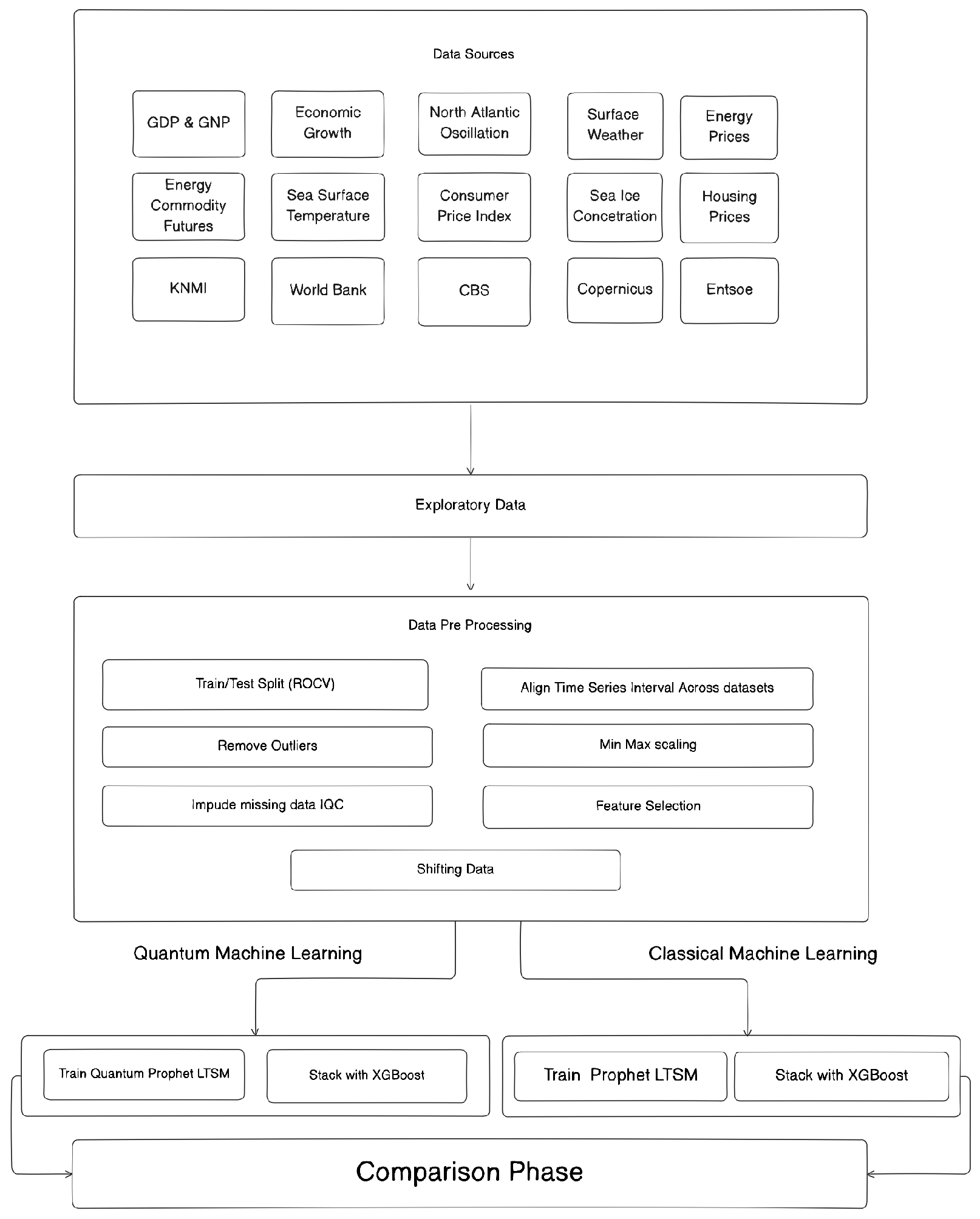
This section proceeds in three steps. First, we present the materials, data sources, and exploratory checks (
Section 3.1;
Table 1). Second, we detail the methods, preprocessing and feature engineering (
Section 3.3); model architectures (Prophet, LSTM, QLSTM) and stacking; and training/tuning (
Section 3.6). Third, we describe the evaluation protocol and reproducibility setup, including rolling-origin cross-validation (
Section 3.7.4). The overall pipeline is summarised in
Figure 1.
In line with SQ1–SQ4, the design tests whether integrating climate and macroeconomic predictors within a Prophet–(Q)LSTM residual architecture reduces long-horizon forecast error relative to classical baselines under rolling-origin validation.
3.1. Data Collection
Drawing on the findings of
Section 2, we group our predictor variables into two domains. The first domain,
macroeconomic activity, and price dynamics, includes time series on the gross domestic product (GDP), labour participation, the consumer price index (CPI), housing prices, end-user energy prices, and international commodity prices. The second domain,
climate variability, is represented by local surface-weather observations and large-scale indices such as the North Atlantic Oscillation (NAO), North Atlantic sea-surface temperature (NAT), and sea-ice concentration (SIC). The primary target variable is the hourly electricity load in The Netherlands, obtained from ENTSO-E. This load series defines the supervised learning target throughout the forecasting task.
Raw data were collected from five open-access providers in Spring 2025. CBS macroeconomic tables were downloaded manually as CSV files between 22 January and 16 April 2025. Monthly commodity-price series were obtained from the World Bank “Pink Sheet” on 10 June 2021. Daily weather observations for the station “De Bilt” were retrieved from the KNMI Data Centre on 12 March 2025. ERA5 climate reanalysis data were accessed the same day via the Copernicus Climate Data Store API in NetCDF format. The NAO index was downloaded as a fixed-width text file.
Hourly electricity load data were extracted from the ENTSO-E Transparency Portal on 30 March 2025, comprising CSV files and an Excel archive covering 2006–2015.
While original data have a wide span (e.g., NAO: 1950–2025; CPI: 1996–2025), only the period 2010–2024 was used for training and evaluation, aligning all predictors with the availability of hourly load data. No data cleaning, resampling, or interpolation was performed at this stage; subsequent steps are detailed in
Section 3.3. The selected sources jointly cover long-horizon macroeconomic dynamics and shorter-horizon climate and weather variability that theory and prior work identify as key drivers of national electricity demand while ensuring public availability and reproducibility.
These choices encode the substantive relationships examined throughout this study: (i) local weather and large-scale climate signals as physical drivers of hourly load; and (ii) macroeconomic activity and price dynamics as demand and price-elasticity channels. We expect colder conditions and stronger economic activity to be associated with higher consumption, while higher end-user energy prices may dampen demand. The ensuing methods test whether combining these signals improves long-horizon forecastability.
3.2. EDA
Due to the diverse and vast amount of datasets that needed to be considered, the EDA played an essential role in reducing the dimension of the data, since the goal is to create one dataset that represents the most information in the smallest package. The first problem that was tackled was the difference in time intervals between the datasets. Most of them had monthly or yearly intervals but needed to be formatted to hourly intervals to be combined with the target variable data.
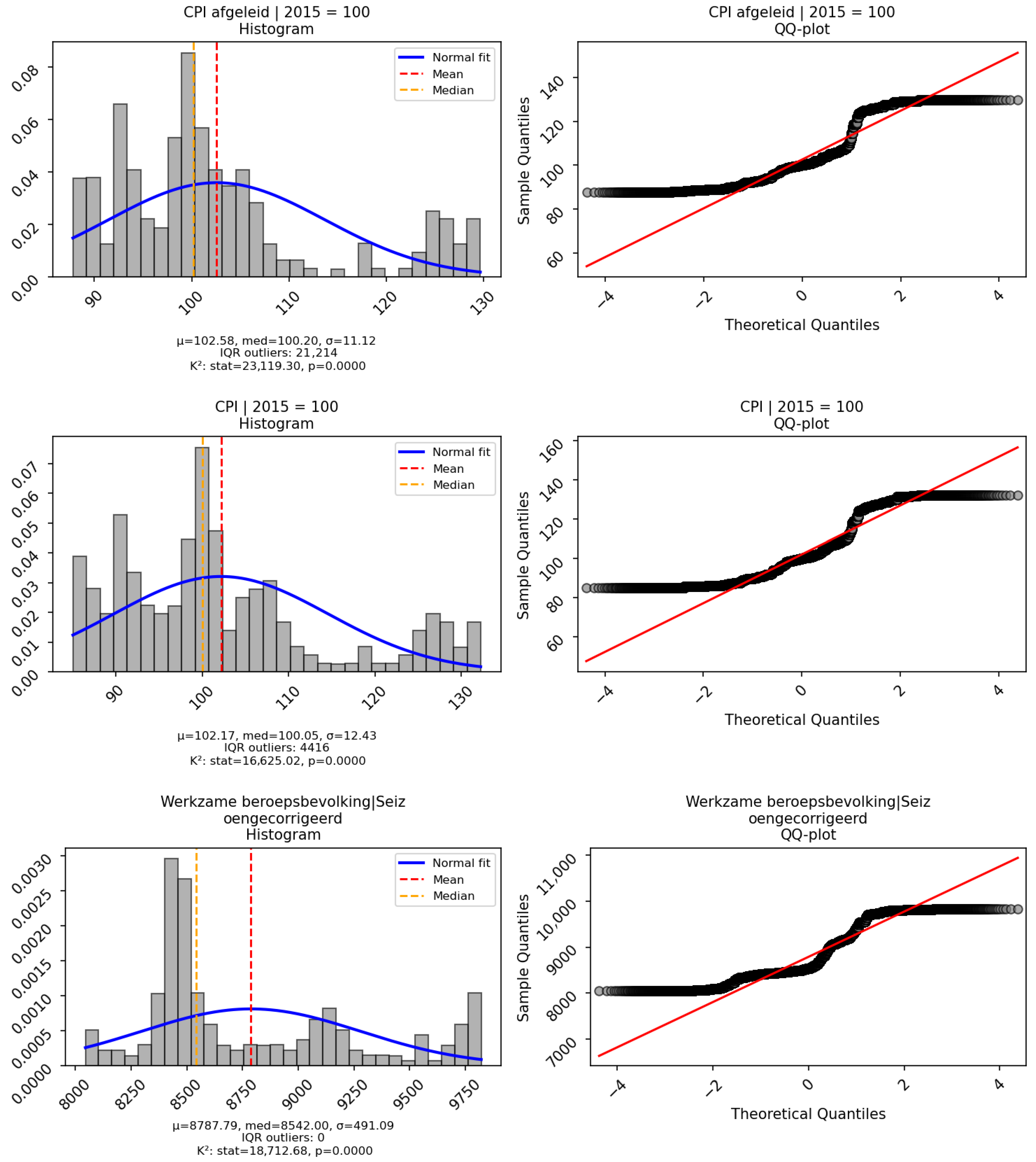
The second challenge was to check the normality and distribution. This was performed by creating a Q–Q plot and a distribution plot. Lastly, we examined the overall health and quality of the data by exploring the amount of missing data and outliers between the datasets. A comprehensive summary of data health appears in
Table 2 below.
Apart from moderate gaps in year-on-year change columns (3.5%), four commodity subseries (≤0.37%), and the NAO index (1.2%), there were no missing data. All NaNs reported in
Table 2 were imputed with multivariate MICE after outlier removal.
The 53.85% missing rate reported for the work-day-corrected GDP refers to pre-1997 observations outside our analysis window. Within the 2010–2024 window used for modelling and evaluation, the GDP subseries that entered the final feature set had complete coverage and therefore did not require MICE imputation; imputation was applied primarily to year-on-year CPI/house-price growth rates, four commodity subseries, and the NAO index (cf.
Table 2).
Based on
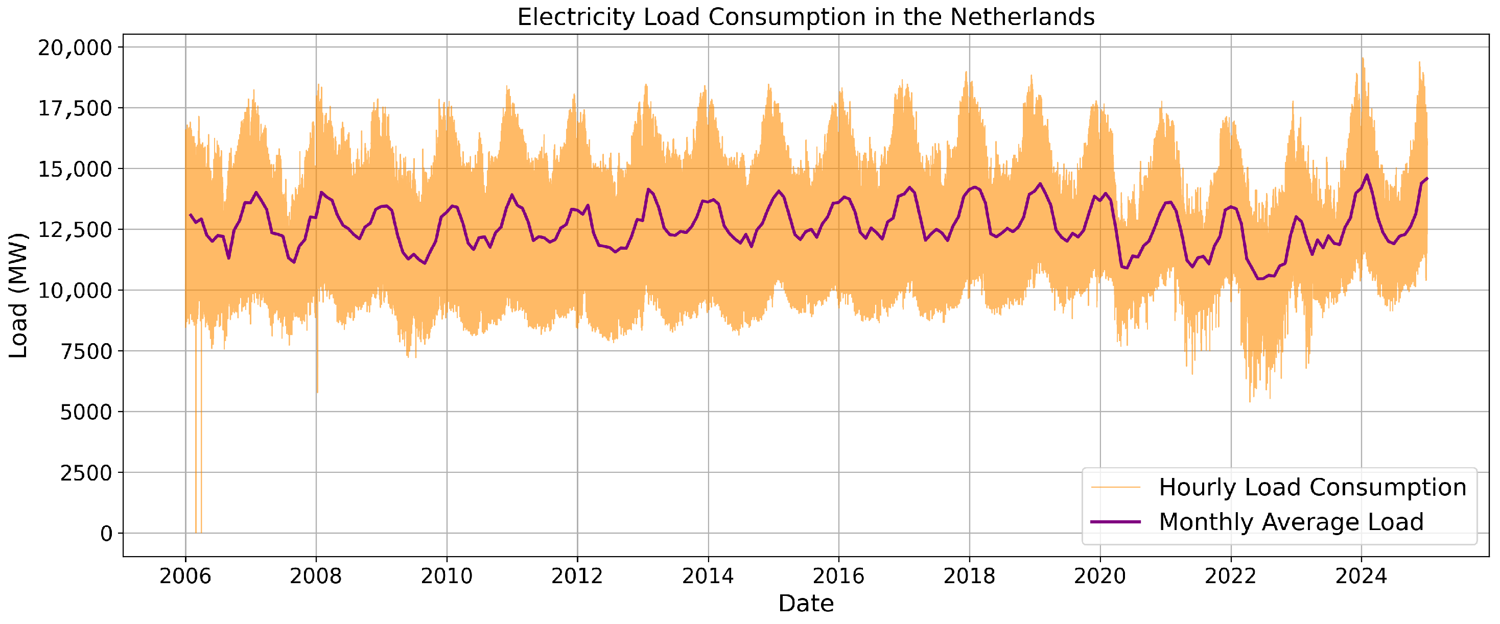
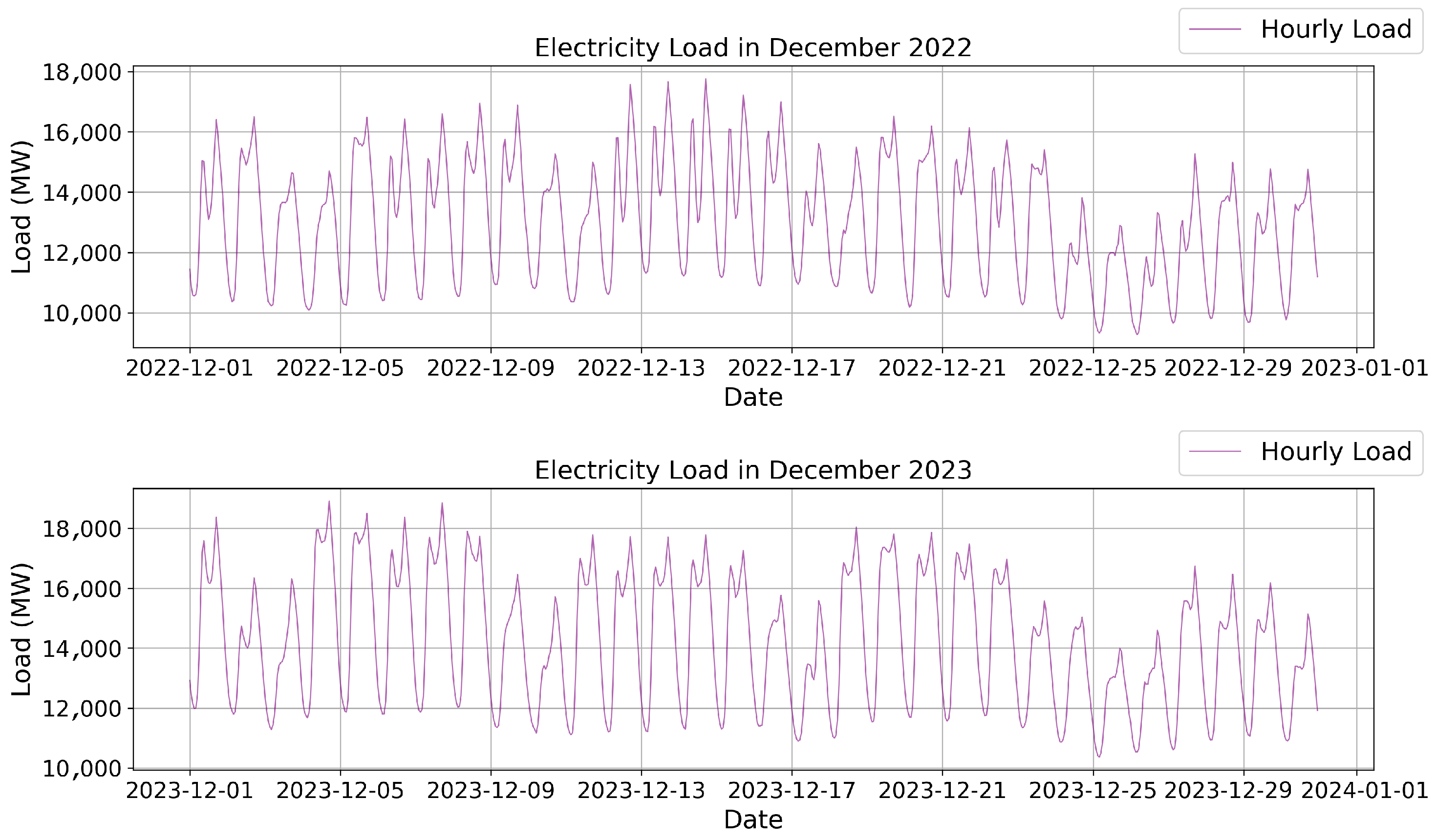
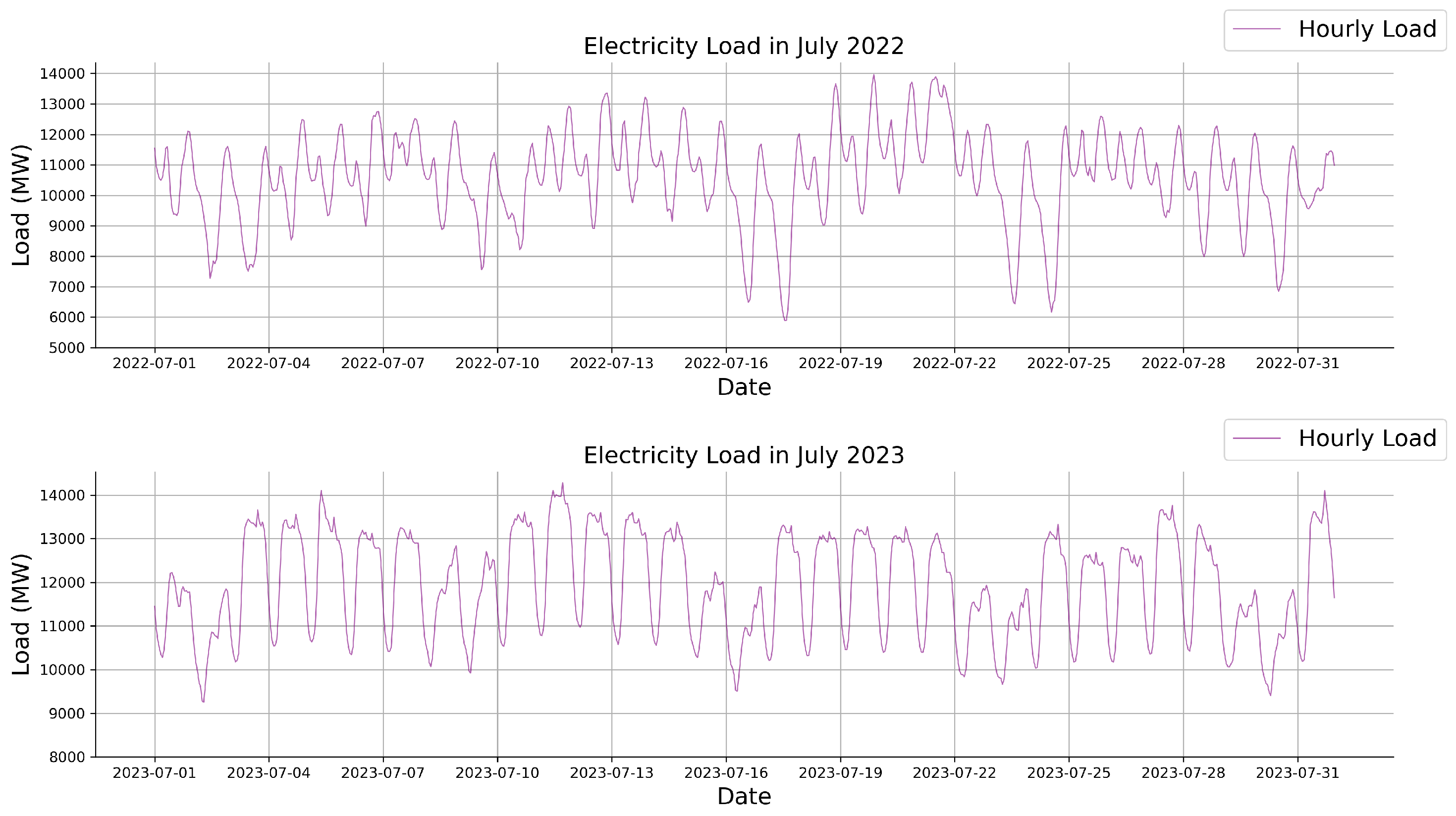
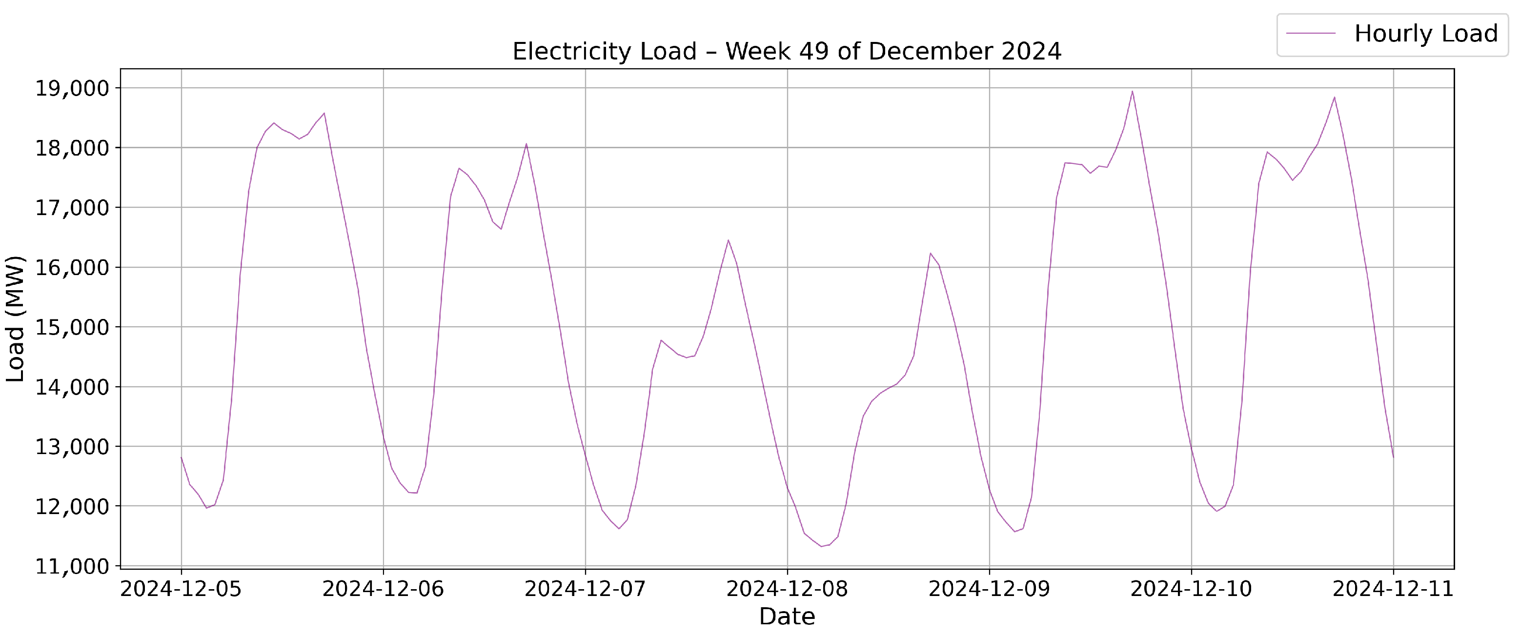
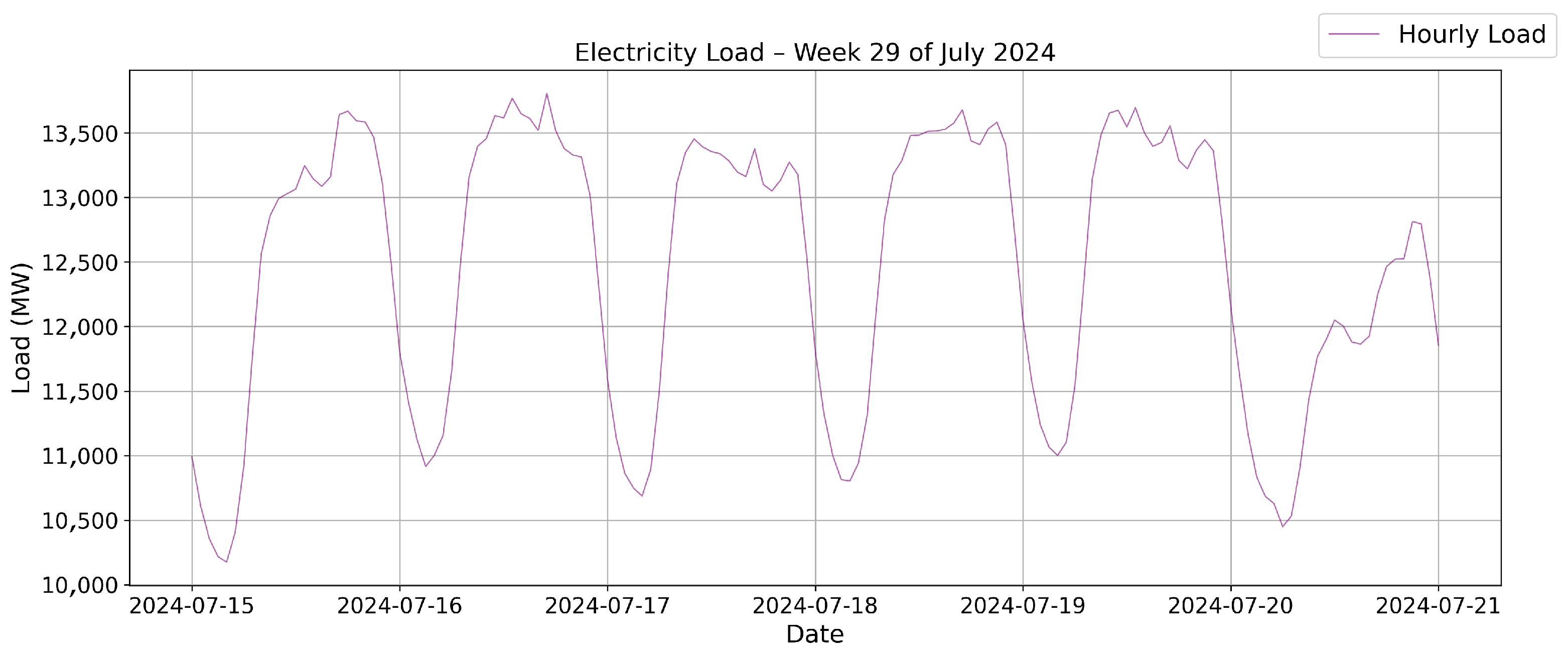
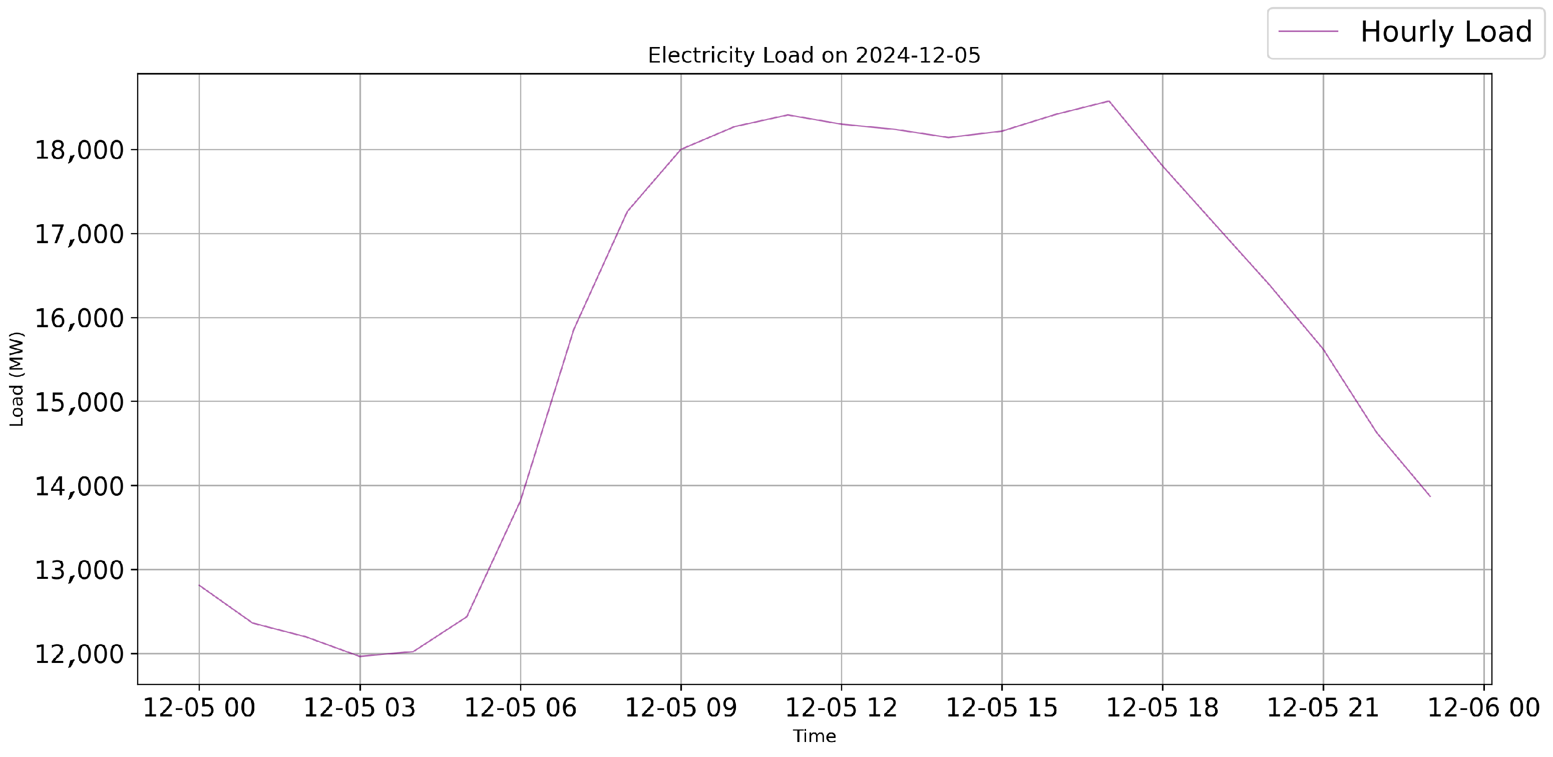
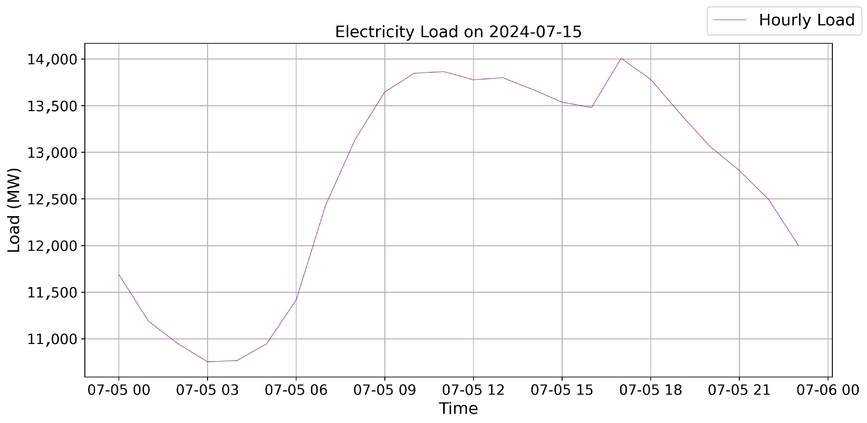
Table 2, we knew that the data quality was good. The work-day-corrected GDP column was the only concern since it shows many NaNs before 1997, but since our train/test data that started from 2010 it did not affect our pipeline. However, we did need to gain a clearer view of the behaviour of the Load Consumption. To do so, we plotted different moments in different seasons. Based on the patterns that emerged in the plot, we can see that the pattern does not change much between summer and winter. However, the peaks of diagrams are lower in the summer compared to their winter counterparts. During the day, we can see a clear rise from 6 a.m. and a gradual decline after 6 p.m., both for the winter and summer days.
To provide a concise visual summary at the month level, we show the monthly average (
Figure 2) and representative winter and summer months (
Figure 3 and
Figure 4).
EDA therefore serves two purposes: (a) to reduce dimensionality toward a parsimonious feature set and (b) to verify that the seasonal and diurnal structures the models must learn are stable across years. These diagnostics motivate the feature-balance search and correlation checks reported later.
3.3. Data Preparation
The data preparation pipeline involved systematic quality control, temporal transformations, and scaling to ensure reproducibility and optimal model performance. The following subsections detail these steps precisely.
- (a)
Data-quality control
Missing values. Table 2 reports NaN proportions over the full raw spans of each source. Within the 2010–2024 analysis window, the GDP subseries used in the final models exhibited complete coverage and thus did not require MICE imputation. Gaps occurred mainly in (i) year-on-year CPI and house-price growth rates, (ii) four commodity subseries, and (iii) NAO. These were imputed using Multivariate Imputation by Chained Equations (MICE).
Outlier handling. Values outside were adjusted to the nearest bound (affecting 0.6% of entries).
Type normalisation. Decimal commas were replaced with points; Dutch quarter and half-year labels were converted into pandas.Period objects; numeric strings were cast to floating-point numbers.
Imputation diagnostics. For variables that were imputed, we inspected MICE chain stability and compared pre/post marginal distributions; overlays showed no material shifts relative to the observed portions of each series.
The IQR-based clipping was applied to predictor variables only; the target load series (ENTSO-E) was left unaltered. Diagnostic winsorised variants explored later (
Appendix A.5) did not feed into headline results.
- (b)
Transformations for modelling
Temporal expansion. Annual, quarterly, and monthly data were up-sampled to daily frequency and then replicated hourly, resulting in a uniform dataset from 1 January 2010 to 31 December 2024.
Alignment and merging. Data sources were merged to the load-series index through a custom routine that inferred frequency, forward-filled lower-frequency observations, and removed duplicate timestamps.
Feature engineering.
- -
Calendar decomposition into year, month, day, hour, minute, and weekday features.
- -
Features were selected based on their correlation with the target variable, with the optimal number per domain (economic and climate-related) determined through Bayesian optimisation.
Target alignment. The target series was shifted by 4320 h to ensure accurate temporal alignment and causal integrity.
Scaling. All predictors underwent Min-Max scaling to the range using a single scaler across the dataset.
Preprocessing was performed separately on each fold to prevent data leakage. During the initial model testing and feature selection phases, a temporal split was used to divide the data into training (prior to 2019) and testing (the year 2019) sets. In the final pipeline, however, rolling-origin cross-validation was employed across the entire dataset to provide a comprehensive evaluation of model performance.
3.4. Baseline Models
To benchmark the proposed Prophet–QLSTM models, two baseline models were implemented: the Prophet model and the ensemble Prophet–LSTM model. Both baselines were trained using the same preprocessing pipeline and hyperparameter settings as the Prophet–QLSTM experiments to ensure comparability. Specifically, the Prophet–LSTM model used an LSTM with two layers, having hidden sizes of 60 and 120 neurons, respectively, a sequence length of 48, a learning rate of 0.001, and the Adam optimiser.
The Prophet model provides a robust statistical benchmark by capturing trends, seasonality, and holiday effects inherent in the electricity load data. The Prophet–LSTM model extends this baseline by incorporating an LSTM network trained on Prophet-generated regressors, enabling it to learn complex temporal patterns beyond those captured by Prophet alone [
4]. This ensemble approach is widely used in recent EDF research.
These baselines serve to quantify the additional predictive benefit introduced by the quantum-enhanced QLSTM architecture. Together, these baselines define the counterfactuals for our endpoints: primary (mean RMSE across 13 folds) and secondary (MAPE, PCC).
3.4.1. Prophet
The Prophet model is an additive regression framework designed to capture trends through piecewise linear or logistic growth curves. It combines Fourier series to model yearly seasonal patterns and dummy variables to address weekly seasonality. The framework excels in analysing datasets with extended temporal spans (months or years) containing high-frequency historical data (hourly, daily, weekly), particularly when handling scenarios with:
Multiple pronounced seasonal effects
Known significant but irregular events
Missing data points or outliers
Nonlinear growth patterns that approach saturation points
Its flexibility makes it robust for forecasting in complex, real-world time series where traditional models may struggle.
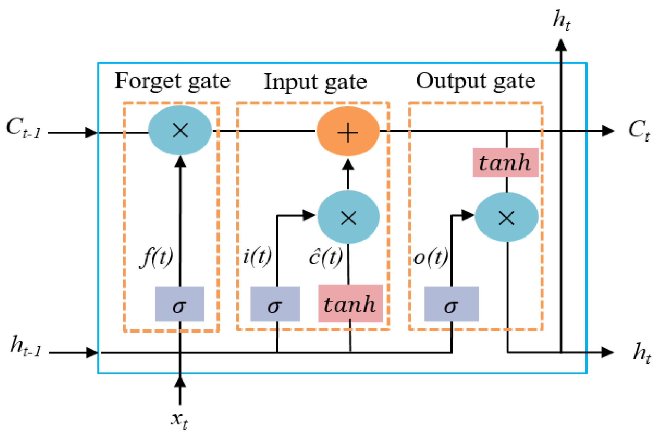
3.4.2. Prophet–LSTM
The widely used solution for solving EDF is using an ensemble method where Prophet is first fit to the load series. After fitting, the generated regressors are used as new features that will be fed into the LSTM as seen in van de Sande et al. [
4]. The LSTM architecture is constructed as seen in
Figure 9.
3.5. Quantum-Enhanced Forecasting Model
Ensemble learning is used to combine the Prophet model with the QLSTM setup. The QLSTM that will be used is an implementation created by Di Sipio [
28], which was utilised in other research such as Khan et al. [
7].
3.5.1. QLSTM
A QLSTM, is a quantum–classical hybrid long short-term memory model. This entails that a classical LSTM has the classical LSTM cells replaced with VQCs, which function as tuneable parameters in the architecture. The VQC task is divided into three layers. The first is the data encoding, this is performed by using the H, Ry, and Rz gates. The second layer is the variational layer; here, the parameters will be tuned. Lastly there is the quantum measurement layer; in this layer, a fixed length vector is returned that represents the expectation values of every qubit [
5]. The full architecture can be seen in
Figure 10.
In our implementation, the variational quantum circuit (VQC) replaces the classical LSTM cell’s affine+nonlinearity transformation. At each time step, the concatenated input
is encoded via single-qubit rotations, evolved by an entangling ansatz, and measured to produce an expectation vector
. Linear maps then form the gate pre-activations,
followed by the usual sigmoid/tanh. Thus, the VQC serves as a learned, compact, nonlinear feature extractor (a data-dependent kernel) that feeds all gates simultaneously. Via entanglement,
can encode higher-order interactions between
with far fewer trainable parameters than a classical dense layer (cf.
Appendix A.1). We do not claim a formal separation from classical LSTM expressivity; rather, we hypothesise benefits in parameter efficiency and long-horizon residual modelling under the fixed feature budget considered here.
The core forecasting model is a two-layer Quantum LSTM (QLSTM) implemented using PennyLane (0.40.0). It is configured as follows:
First Layer: QLSTM with return sequences enabled.
Dropout: Optional dropout is applied between QLSTM layers.
Second Layer: QLSTM with return sequences disabled (final time step only).
Fully Connected Layers: A dense layer followed by ReLU activation and another dense output layer.
The choice of using a hybrid Prophet–LSTM and Prophet–QLSTM architecture was motivated by the complementary strengths of its components. Prophet provides interpretable, decomposable forecasts suited for capturing seasonality, holidays, and trend changes in electricity demand, while LSTM and QLSTM architectures offer the capacity to model complex temporal dependencies and nonlinearities that Prophet alone cannot resolve [
10]. The use of QLSTM was further motivated by its potential to generalize better in low-data or high-complexity settings by leveraging quantum-enhanced representations [
5,
7].
3.5.2. Stacked Generalisation
To prepare for the necessary error correction in quantum computing, both the Prophet and Prophet–QLSTM predictions are fed into an XGBoost regressor model, configured with the following hyperparameters: n_estimators = 100, max_depth = 3, learning_rate = 0.1, and random_state = 42. Stacking the Prophet–QLSTM with Prophet gives us a targeted, interpretable way to correct the unique biases of our quantum model, maximising the ensemble gain where it is most needed. It will also be added to the Prophet–LSTM to see whether or not stacking might also be beneficial for EDF when applied to a non-quantum model.
3.6. Training Setup and Hyperparameter Tuning
All neural network models were implemented using PyTorch (v2.8.0) for classical components and PennyLane (
lightning.qubit backend) for quantum components [
29]. Models were trained using the Adam optimiser with a learning rate of 0.001. Each training session ran for a maximum of 50 epochs with a batch size of 256, employing early stopping with a patience of 5 epochs and a minimum validation loss improvement threshold (
). To ensure reproducibility, experiments were conducted with fixed random seeds, maintaining consistency across both local computing environments and the Snellius HPC cluster. Training involved standardised data loaders to handle sequence batching effectively.
3.6.1. Bayesian Optimisation and Feature Selection
Full Bayesian optimisation over the entire hyperparameter space was computationally infeasible for the Prophet–QLSTM model due to hardware limitations, as each trial exceeded 24 h.
Consequently, tuning was performed using the classical Prophet–LSTM, focusing specifically on the number of economic and climate-related predictors, identified as the most influential hyperparameters.
Using Gaussian-process-based minimisation (
gp_minimize from Scikit-optimise), the optimisation explored combinations ranging from 2 to 10 features per domain across 25 iterations. The objective was to minimise the root mean squared error (RMSE) on a validation set with a forecasting horizon of 770 h. The resulting optimal combination (10 economic and 7 climate-related features) was then adopted for all subsequent Prophet–QLSTM experiments. We did not re-optimise the feature balance specifically for QLSTM or the 4320 h horizon due to simulator cost; instead, we froze the subset and verified that the leading predictors remain stable across folds at 4320 h (
Appendix A.3 Figure A2). This justifies portability of the subset, while we do not claim horizon- or architecture-specific optimality (see
Section 5.5).
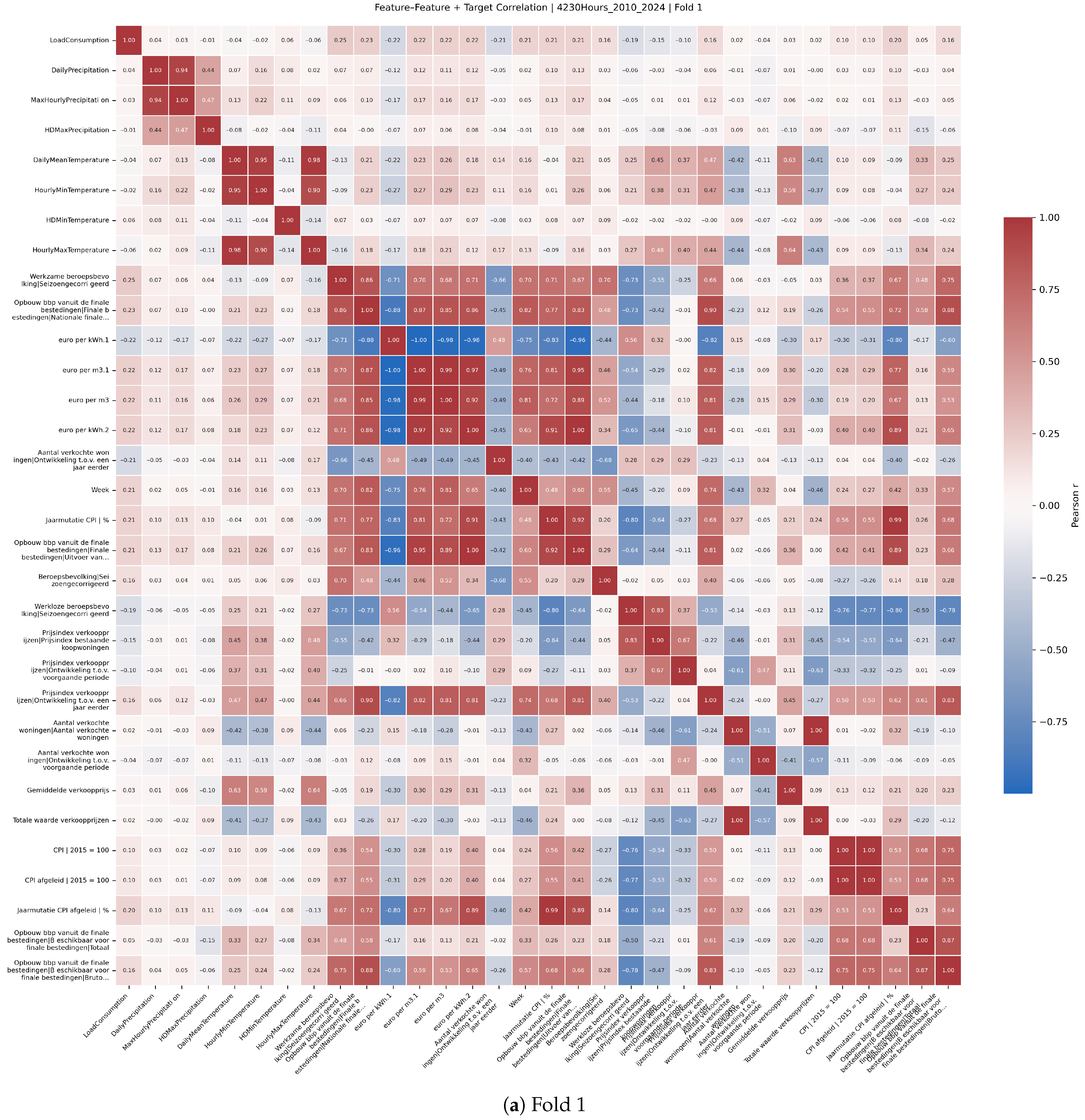
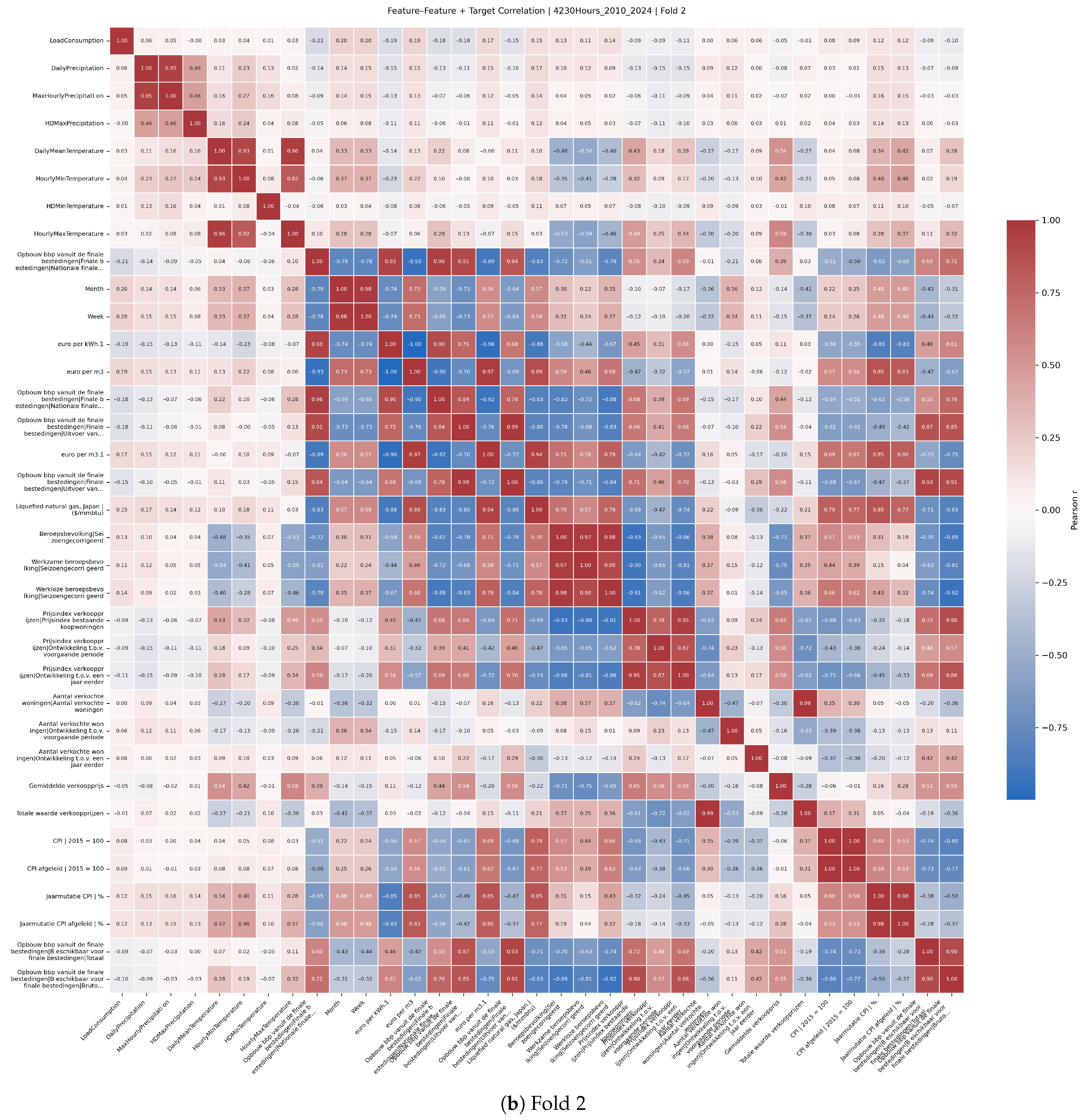
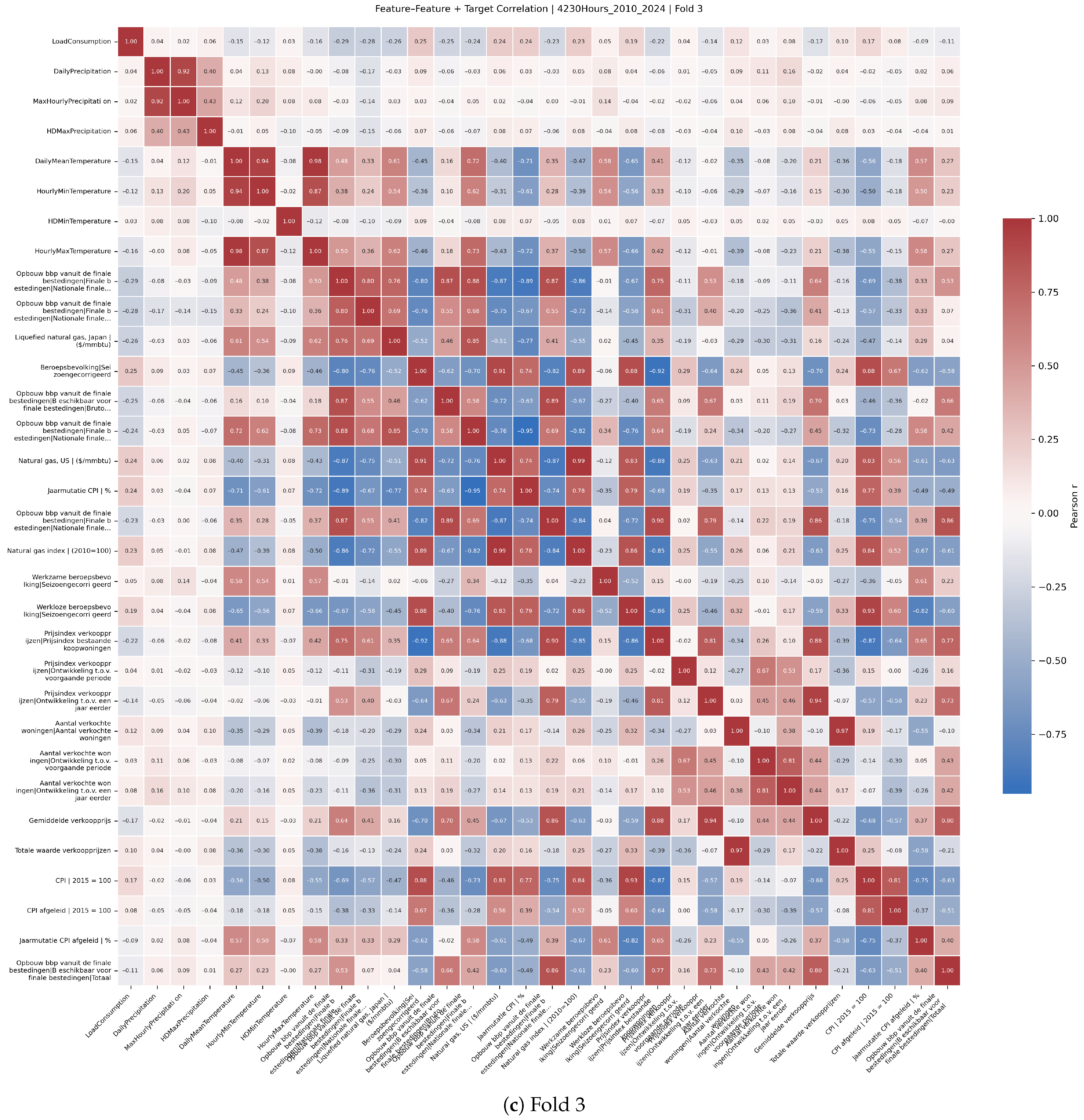
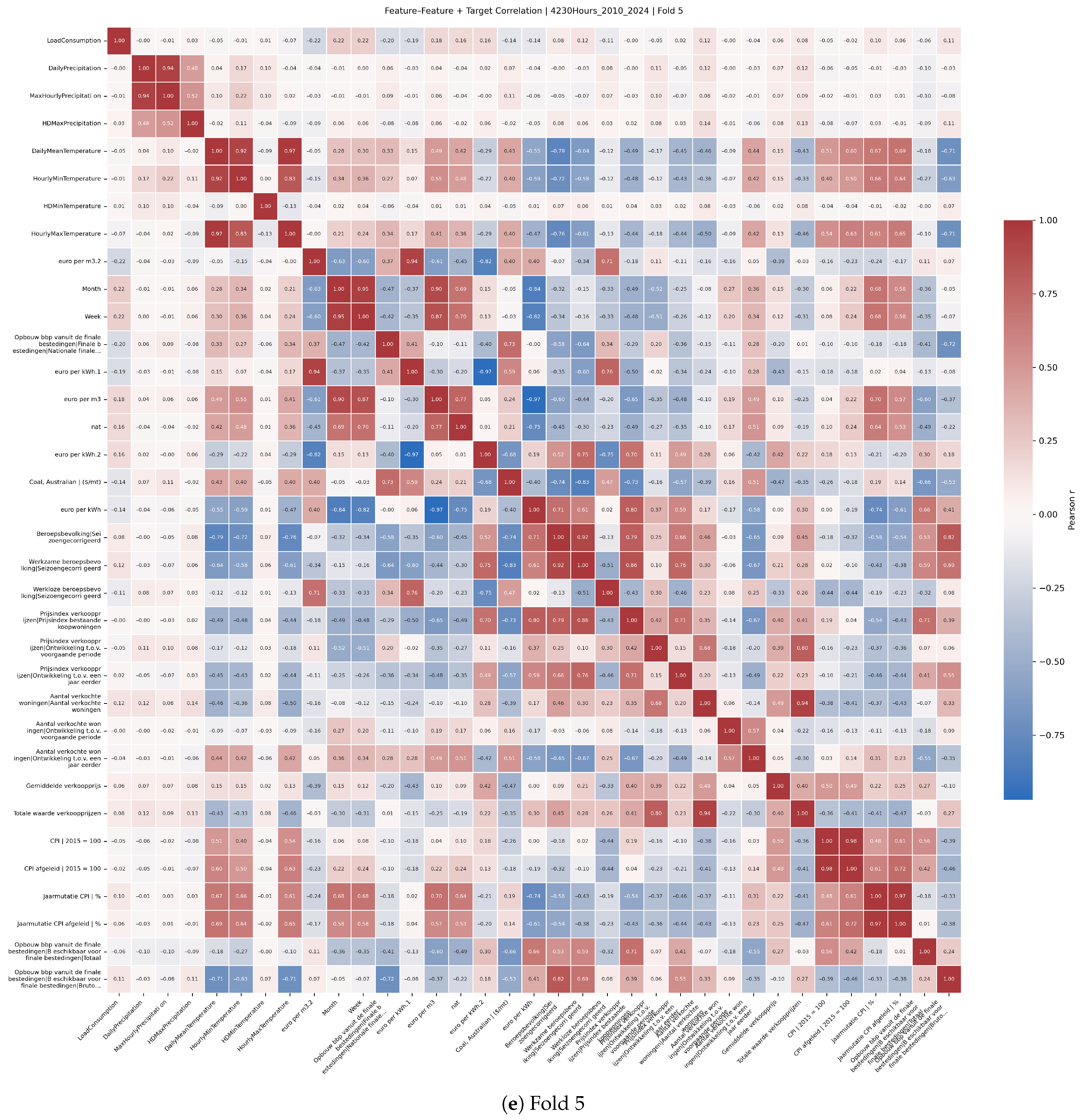
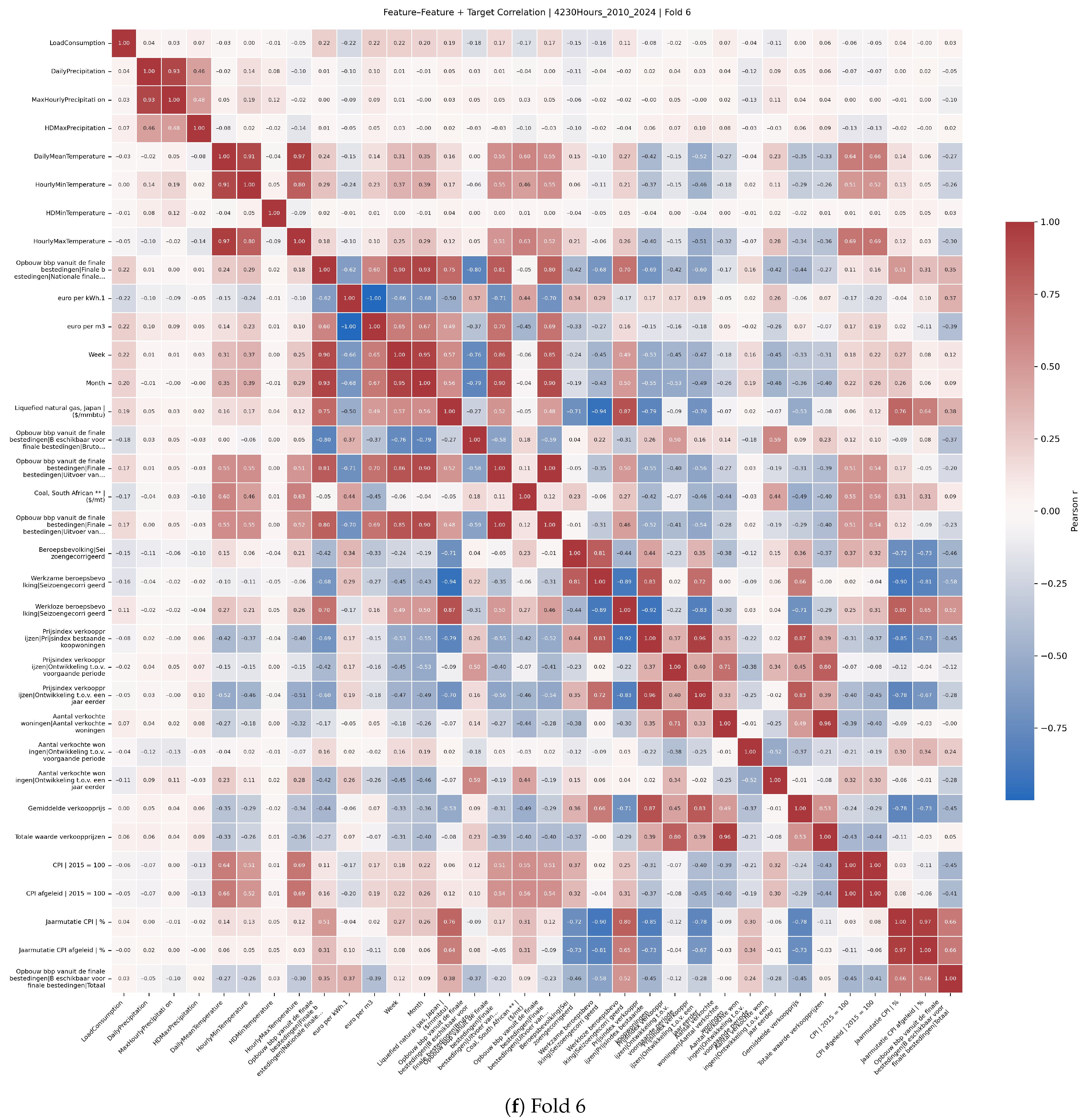
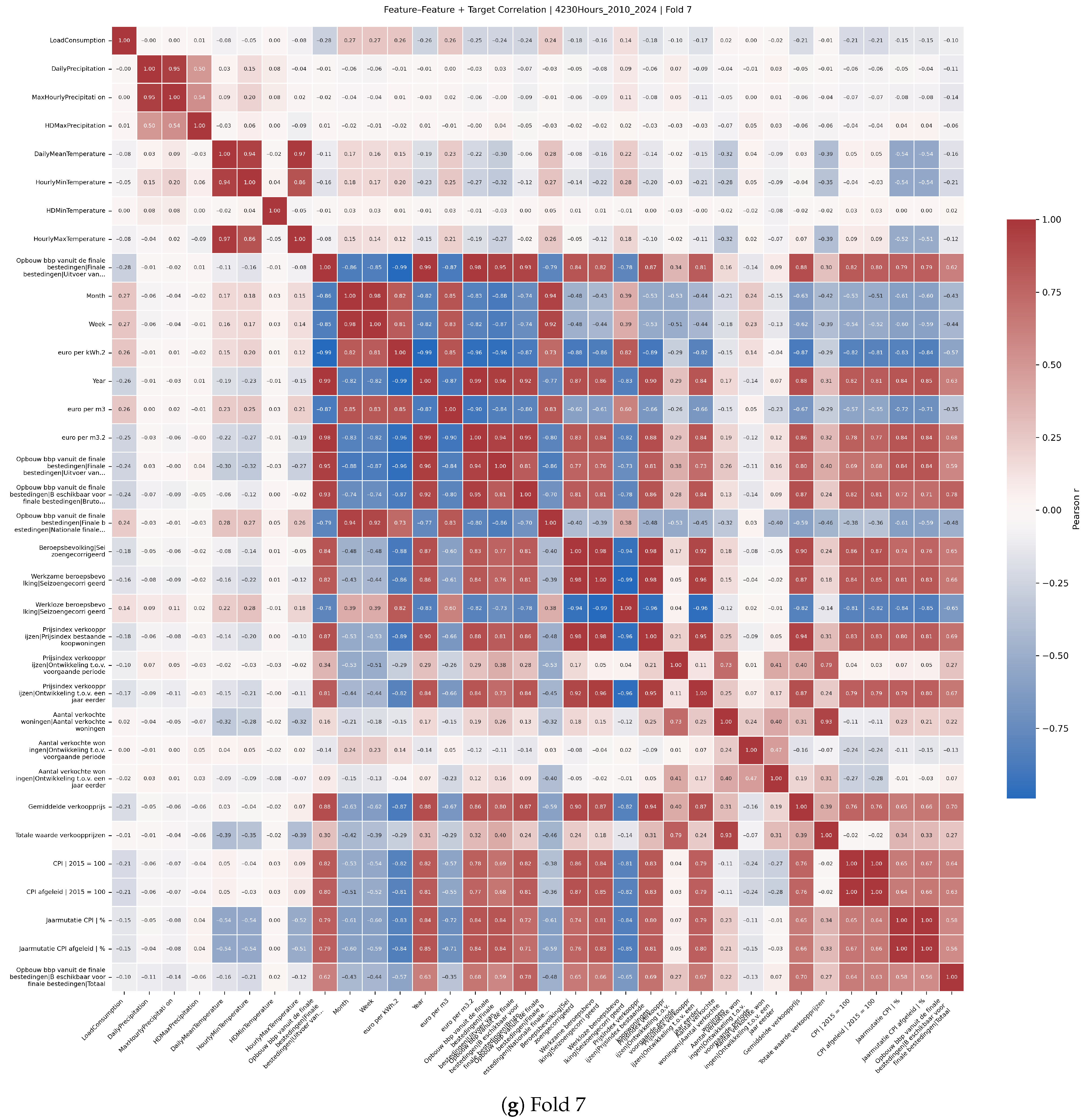
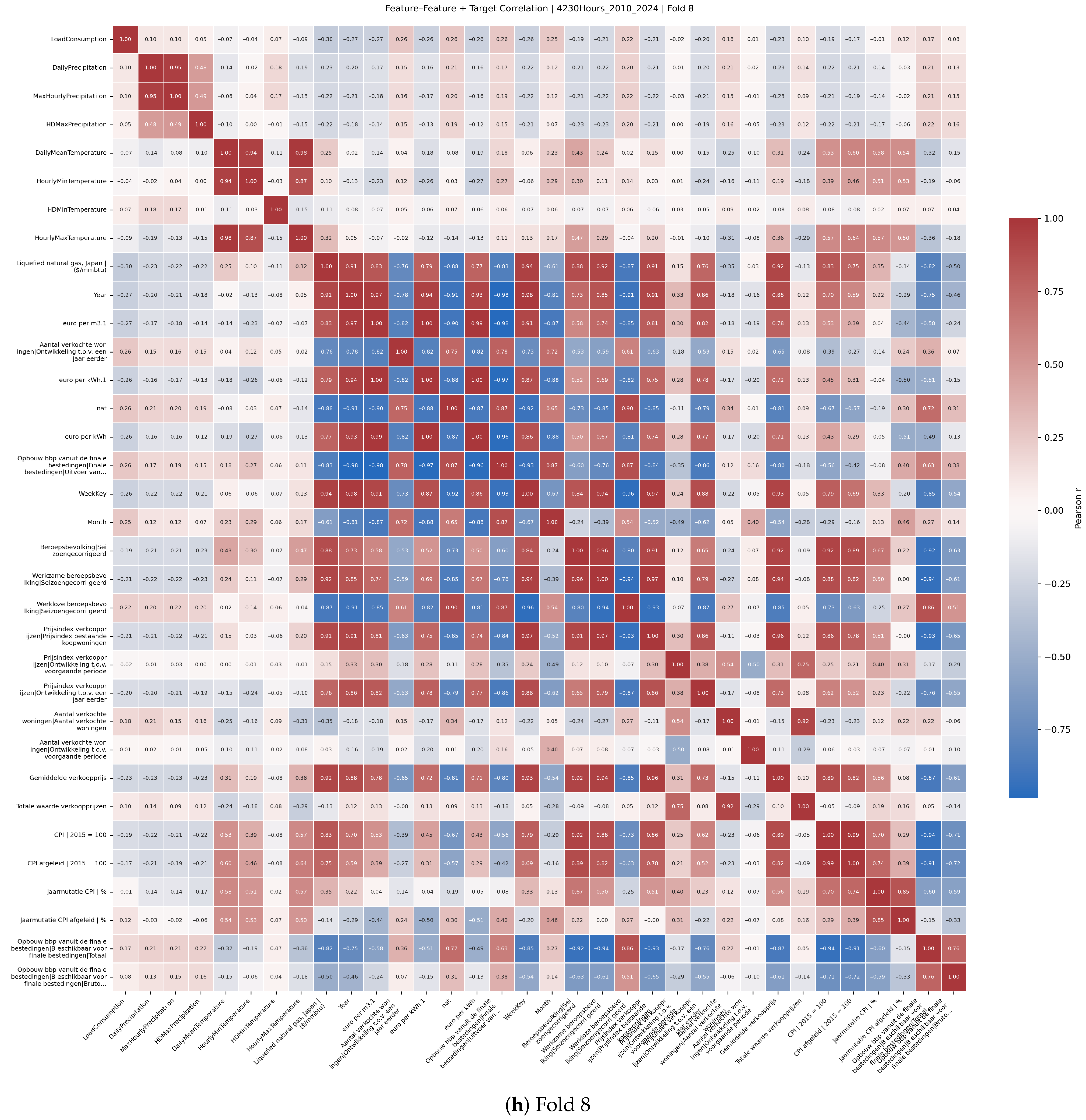
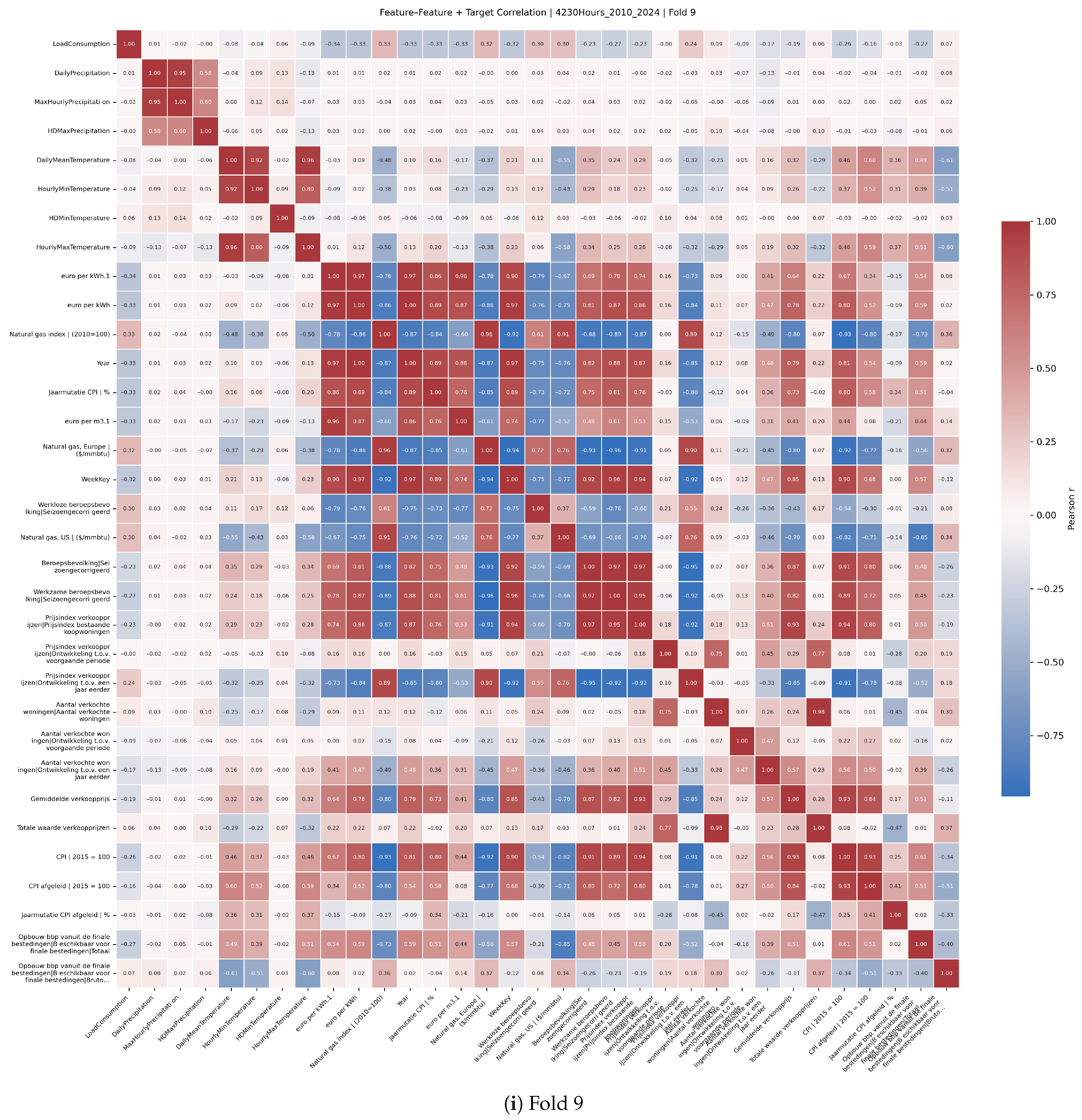
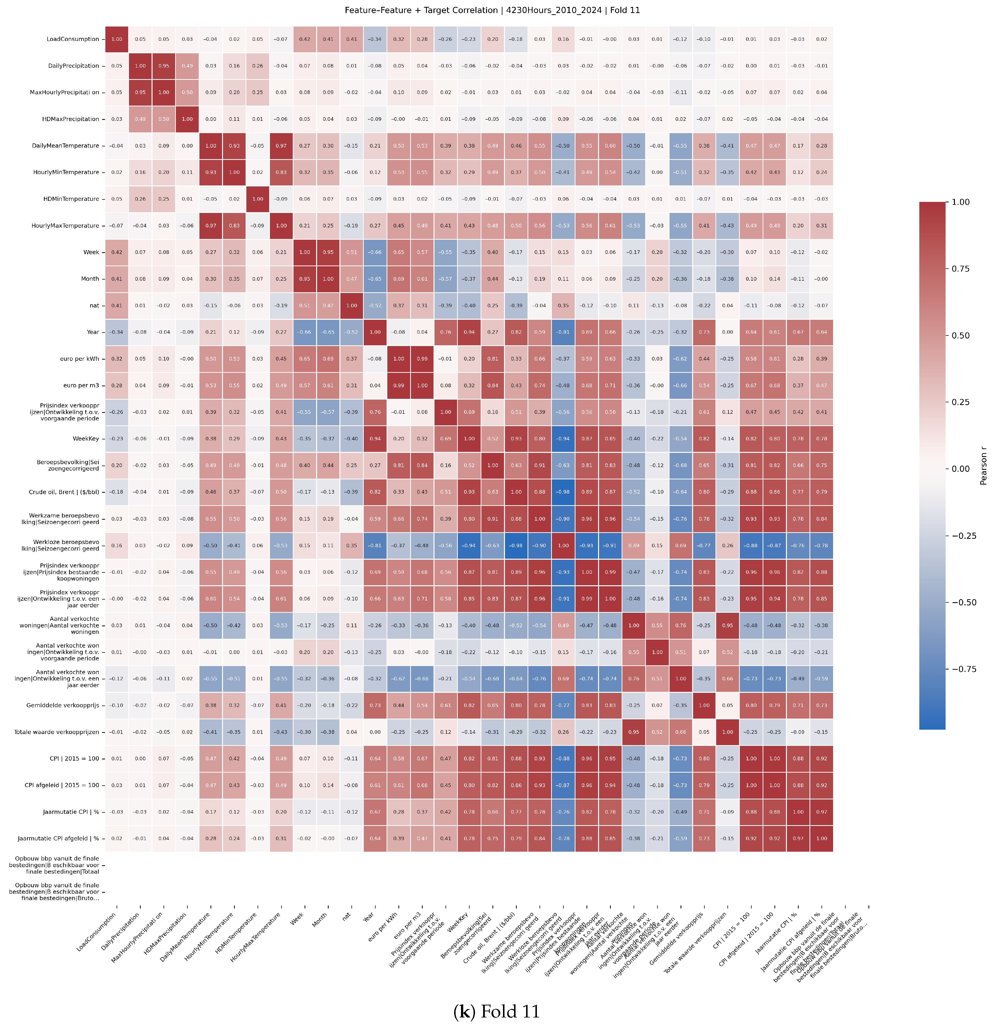
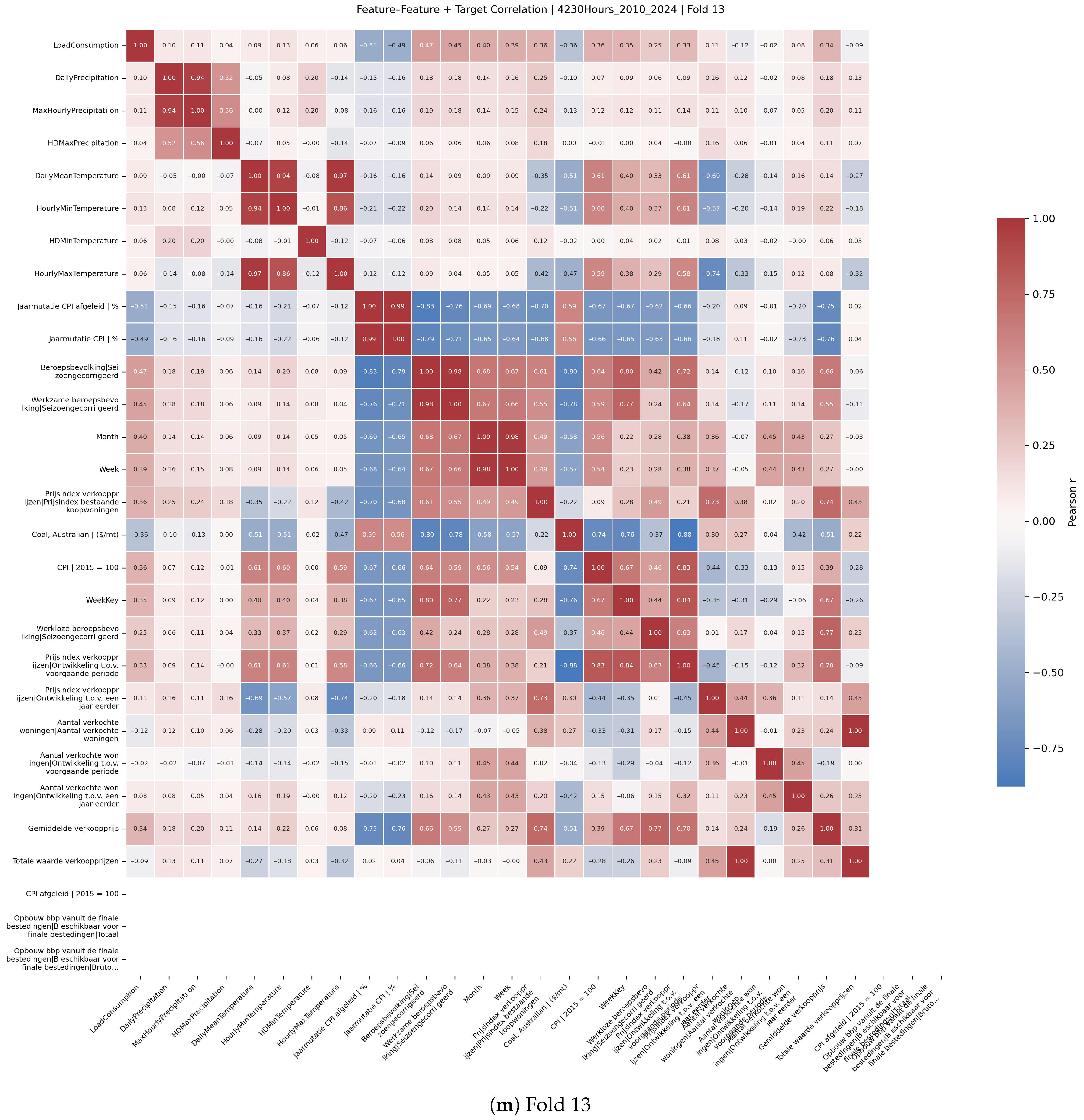
Feature selection was informed by Pearson correlation analyses between predictors and the target variable.
Figure A2 presents correlation heatmaps across multiple rolling-origin cross-validation folds, illustrating stable relationships between key economic and climate variables and electricity demand. These analyses supported the pruning of less relevant features by sorting them by absolute correlation and guided the dimensionality reduction incorporated within Bayesian optimisation.
3.6.2. Configuration
The final configuration utilised the following values as detailed in
Table 3:
3.7. Model Evaluation
To check the performance of the QLSTM model, the following metrics were used.
3.7.1. MAPE
Mean Absolute Percentage Error (MAPE) quantifies the deviation between predicted and actual values as a percentage, offering an intuitive measure of model performance. However, despite its widespread use, MAPE has well-documented limitations, particularly when actual values approach zero. In such cases, the denominator of the MAPE formula becomes very small, resulting in disproportionately large error values that can distort the overall evaluation. To address this issue and provide a more balanced assessment, additional metrics such as RMSE and PCC are included.
3.7.2. RMSE
Root mean squared error (RMSE) depicts the difference between the predicted value and real value and is therefore a useful benchmark to generalise performance between models.
3.7.3. PCC
The Pearson correlation coefficient (PCC) showcases the relation between the predicted load consumption and the real one. This means that it is a good indicator during training to see whether or not the model is picking up the right rhythm in the data and thus helps to interpret trends. However, on its own it is not that useful, but it helps in identifying the healthiness of the other metrics.
3.7.4. Rolling-Origin Cross-Validation
A thirteen-fold ROCV was used throughout tuning and evaluation. Fold k trains on and tests on . Within each training span, the last calendar year is reserved for early-stopping/Prophet tuning. The remaining years form the fit set.
3.8. Hardware
To ensure reproducibility across different computational environments, all experiments were conducted both locally and on the Snellius High-Performance Computing (HPC) cluster. The training configurations, including hyperparameters, random seeds, and software libraries, were kept consistent between these environments. Differences were limited to hardware-specific factors such as batch processing speeds. No changes were made to model architectures or training parameters. This consistency ensures that results are comparable regardless of the computing platform used.
3.9. Experiments
Due to the novelty of utilising a quantum simulation, this study incrementally increased the complexity of the models. This way, we could have a better estimation on the computational resources required when eventually deploying to the HPC cluster. We started off with a minimal viable version of the Prophet–QLSTM setup where we utilised just two qubits and a single layer. We then moved on to four, and at eight qubits the training time per epoch became too high, so the configuration was set to four qubits. Afterwards we tried increasing the number of quantum layers to two, but unfortunately that also led to a resource bottleneck. To determine the horizons that would be feasible for the Prophet–QLSTM we decided to also incrementally increase the horizon. The initial horizon was 770 h, then it increased to 1440 h, and eventually the model was extended to a 4320 h horizon (180 days). For the date range, we first split the data into 2010–2019 and 2019–2024 to avoid computational overload and to see what the impact of the pandemic was on the EDF performance. The size of the folds did not affect performance or resource use as much as expected, so the final run was conducted on the full range from 2010–2024.
We explicitly analysed the 2010–2019 and 2019–2024 windows to gauge the impact of the COVID-19 shock and then ran thirteen-fold rolling-origin cross-validation over 2010–2024. We retained pandemic-period observations and did not apply bespoke outlier removal to the target; instead, Prophet change points and the stacking meta-learner were used to adapt across regime shifts while preserving realism.
4. Results
4.1. Forecast Accuracy of Prophet–(Q)LSTM
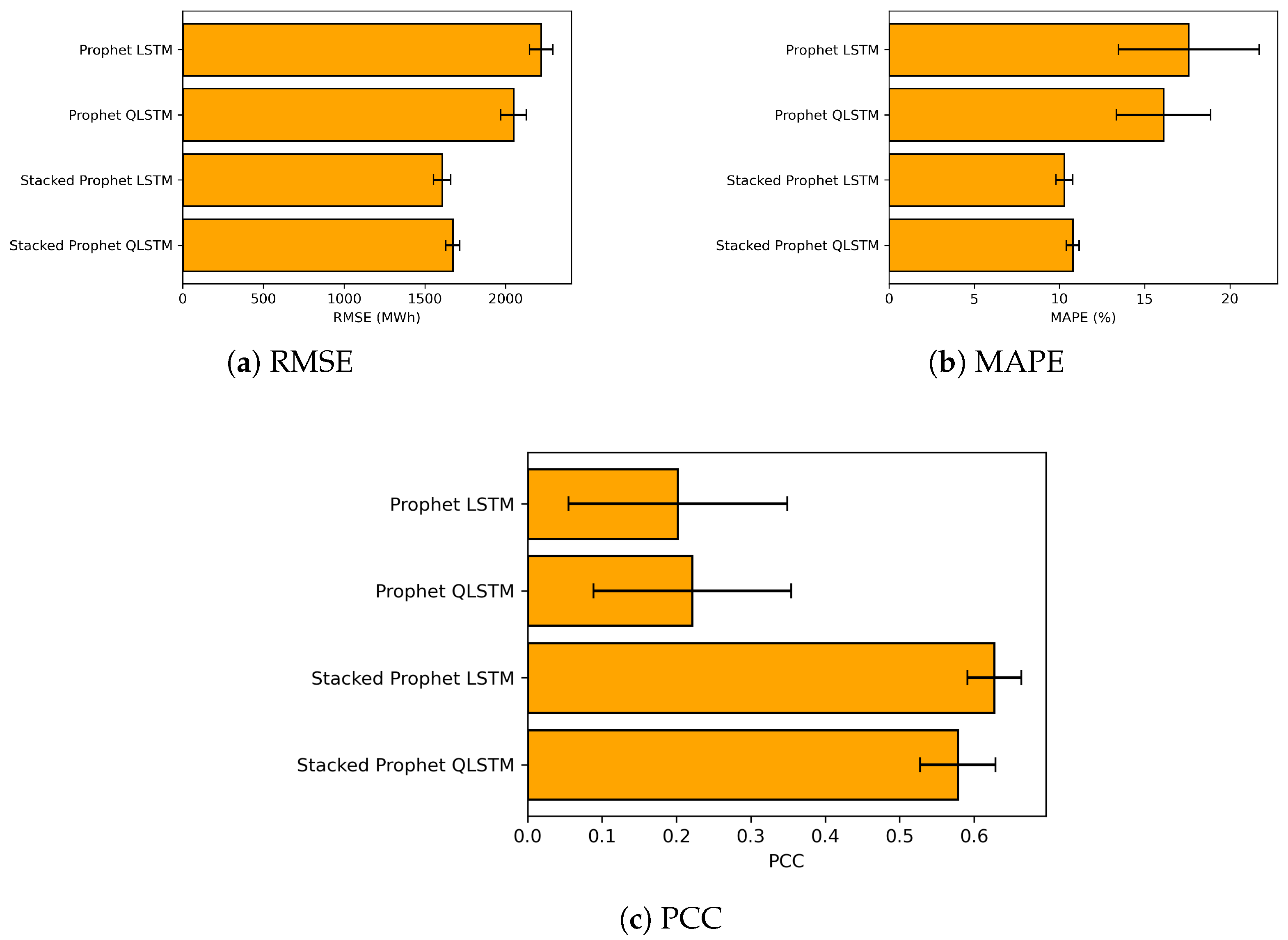
We assess each model’s predictive quality on three complementary metrics: RMSE, MAPE, and PCC. All numbers come from the same 13 rolling-origin test folds used throughout this study.
Table A3,
Table A4 and
Table A5 in
Appendix A.3 provide the fold-level statistics behind
Figure 11. Normality was checked with the Shapiro–Wilk test; wherever it was rejected, 10,000-sample bootstrap confidence intervals are reported.
Key findings
RMSE falls from 2219 MWh to 1606 MWh for Prophet–LSTM (a 27% reduction) and to 1673 MWh for Prophet–QLSTM (24%). The differences are statistically significant ().
RMSE, MAPE, and PCC gaps between the two stacked models stay inside their 95% confidence intervals (); the LSTM stack reaches a slightly higher correlation with the target (PCC + 0.05).
PCC increases to 0.63 for the LSTM stack and 0.58 for the QLSTM stack; the small gap () is linked to residual smoothness.
Prophet–QLSTM beats the classical Prophet–LSTM by 170 MWh RMSE (about 8%;
) while using
fewer recurrent parameters (
Section 4.4).
While stacking consistently outperforms non-stacked variants, the two stacked models are statistically comparable on RMSE and MAPE: the mean RMSE gap (Stacked LSTM vs. Stacked QLSTM) is 66.94 MWh with
, and the mean MAPE gap is 0.48 percentage points with overlapping 95% CIs (
Table A3 and
Table A4). In
Figure 11, the whiskers for the stacked variants overlap for RMSE and MAPE, indicating that improvements between the stacks are often within uncertainty bands. By contrast, the PCC difference (0.63 vs. 0.58) is small yet borderline significant (
;
Table A5), suggesting a modest correlation edge for the classical stack. Taken together, gains from stacking are clear relative to non-stacked models, whereas differences between the stacked variants are frequently marginal and fold-dependent.
Dispersion across folds is larger when the test window overlaps 2020; compare the whisker widths in
Figure 11 and the per-fold RMSEs in
Table A1. Stacking narrows these intervals for both cores, indicating improved stability in turbulent years, while some gains between stacked variants remain within overlapping confidence bands.
4.2. Effect of Integrating Quantum Components
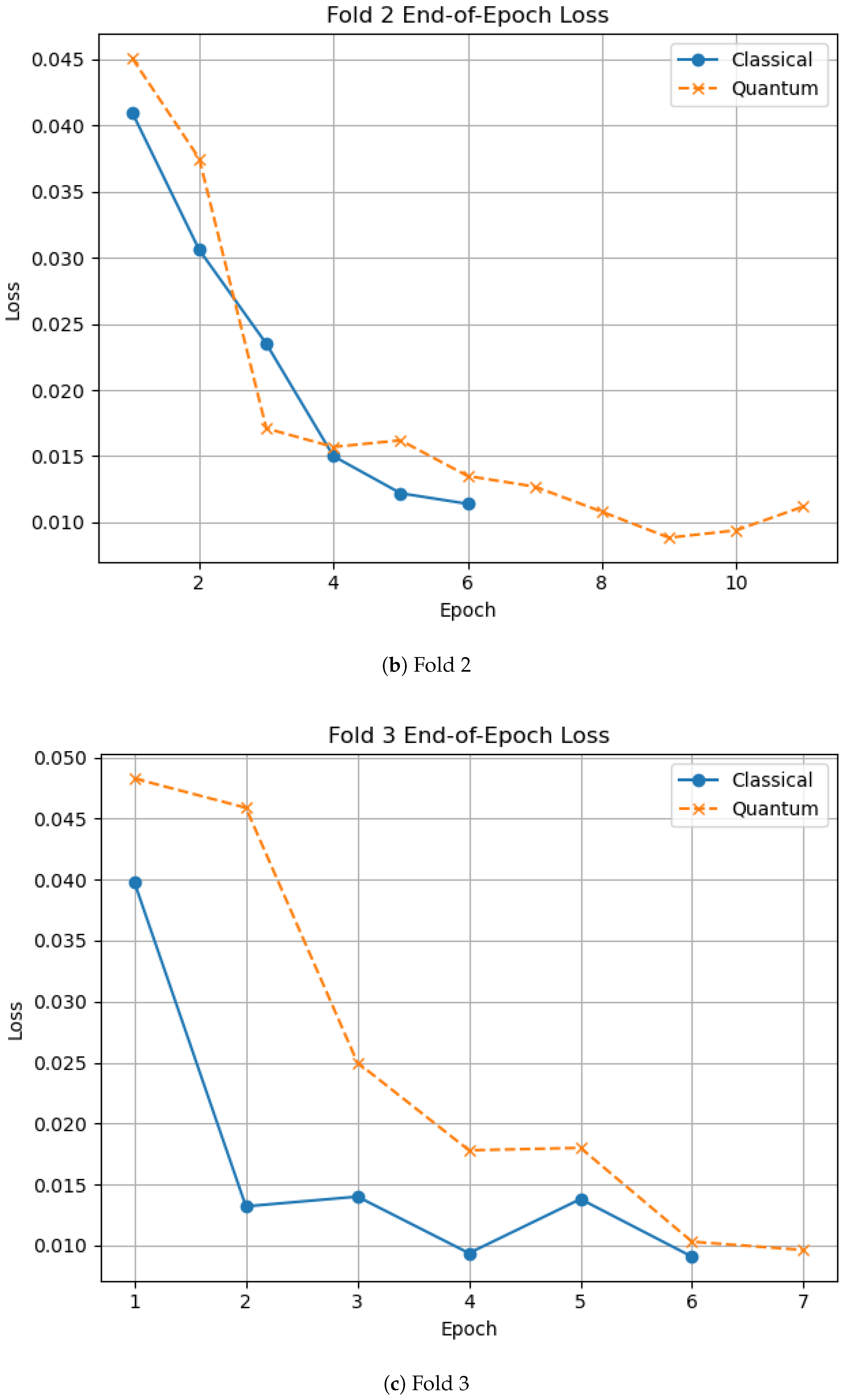
Figure 12 shows the
end-of-epoch loss trajectories for the classical and quantum variants, averaged over the 13 rolling-origin folds, with 95% confidence intervals. Across folds, the quantum run typically stops one epoch sooner than the classical baseline (median stop epoch: 6 vs. 7); an outlier occurs in fold 10, where the classical model continues to epoch 39 before early stopping.
Despite the longer training window, the classical variant converges to a slightly lower loss:
(95% CI) versus
. The overlapping confidence bands indicate that, while the classical model attains the minimum loss on average, the quantum run reaches a loss that is statistically indistinguishable from the classical variant, which is consistent with the RMSE parity reported in
Section 4.1.
4.3. Most Relevant Predictors
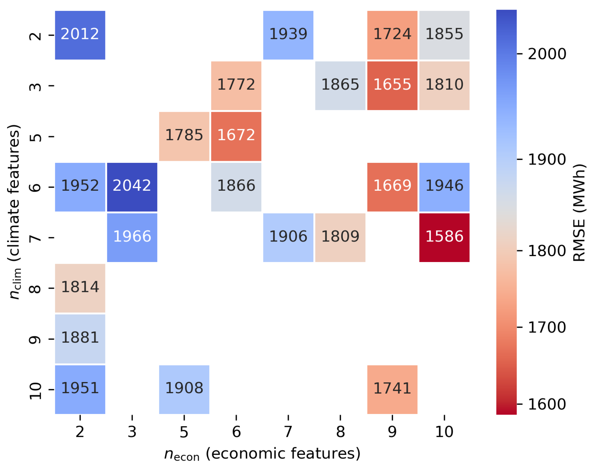
Based on the Bayesian-optimised grid search,
Figure 13 shows a clear response surface. Once the combined predictor count in each domain exceeds seven, cross-validated RMSE reliably drops below 1800 MWh. The improvement is driven mainly by the economic block: RMSE degrades far more when the economic feature count is low than when the same shortfall appears in the climate block.
Figure A2 (4320 h horizon) shows that the top-ranked economic and local-weather variables recur across folds, supporting the use of the 10 + 7 subset selected at 770 h. We therefore keep the feature set fixed across cores and horizons in this study; validating QLSTM- and horizon-specific optima is deferred to future work.
4.3.1. Climate Features
All folds included the following climate features:
Daily mean temperature
Daily precipitation
HD max precipitation
HD min temperature
Hourly max temperature
Hourly min temperature
4.3.2. Economic Features
Earlier folds included:
Gas price
Electricity price
- (a)
Euro per kWh1
- (b)
Euro per kWh2
Coal
Oil prices
- (a)
Crude Oil Average Bbl
- (b)
Crude Oil Brent Bbl
- (c)
Crude Oil Dubai Bbl
- (d)
Crude Oil WTI Bbl
Later folds (with more training data) included:
GDP composition (multiple detailed subseries)
Price index data (e.g., housing prices, transaction values)
Workforce participation (seasonally adjusted)
4.3.3. Prophet-Derived Features
The following Prophet components were included as features in all (Q)LSTM variants:
4.3.4. Generic Date/Time Features
The following calendar-based features were also included:
4.4. Trade-Offs Between Hybrid and Classical Models
4.4.1. LSTM
The PyTorch implementation stores an input–hidden matrix, a hidden–hidden matrix, and two bias vectors per gate; with
and
, this yields 18,960 parameters. See
Appendix A.1 for the full derivation.
4.4.2. QLSTM
Using the PyTorch–PennyLane hybrid layer (, , ), the core contains just 628 trainable weights.
4.4.3. Compute
Time
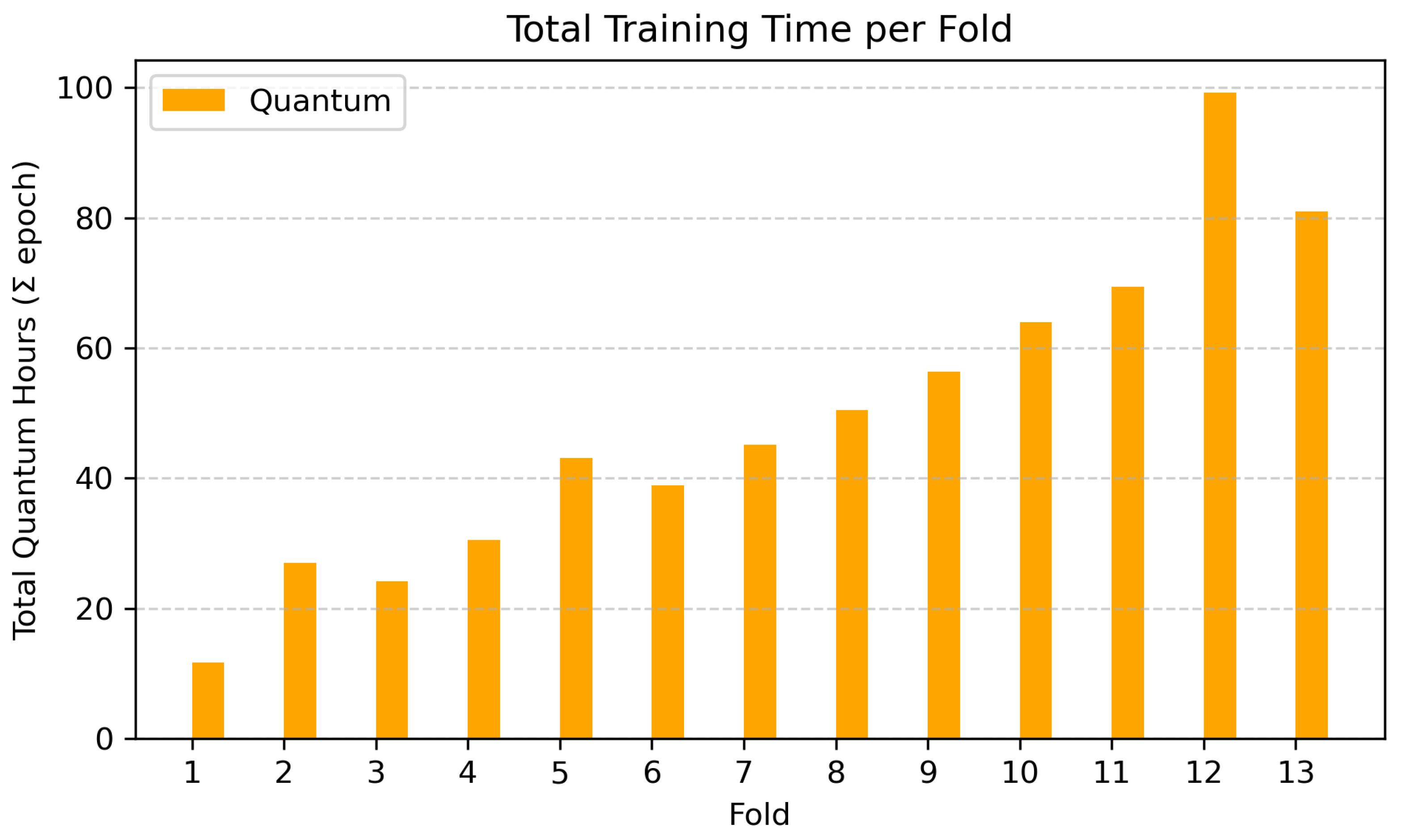
On average, the Prophet–LSTM model completed training within minutes. In contrast, Prophet–QLSTM required at least 1.5 h, and for larger folds several days (see
Figure 14).
5. Discussion
5.1. Effectiveness of Stacking
This research concludes that a stacked Prophet–(Q)LSTM model significantly outperforms the classical Prophet–LSTM in forecasting performance. Specifically, the stacked Prophet–LSTM lowers the mean RMSE by 613.45 MWh, the MAPE by 7.28%, and raises the PCC by 0.43 compared to the baseline, all with statistically significant results (). The stacked Prophet–QLSTM also shows significant improvements, with a mean RMSE reduction of 546.51 MWh, a MAPE reduction of 6.80%, and a PCC increase of 0.38 over Prophet–LSTM, again with .
There is no statistically significant difference between the stacked Prophet–LSTM and stacked Prophet–QLSTM in RMSE and MAPE, although the quantum variant is numerically slightly superior. However, when looking at PCC, a small but statistically significant difference is found (), favoring the stacked Prophet–LSTM. To examine the correlation drop, we also compared the non-stacked Prophet–LSTM and Prophet–QLSTM; no significant PCC difference emerged (). This suggests that the drop in PCC is not due to the use of QLSTM itself but rather a consequence of the stacking process. Notably, Prophet–QLSTM uses about 29× fewer trainable parameters, yet training is slower because the quantum component is simulated.
5.2. Forecast Accuracy of Prophet–QLSTM vs. Prophet–LSTM
When comparing the standalone Prophet–LSTM and Prophet–QLSTM models, the Prophet–QLSTM significantly outperforms the Prophet–LSTM in terms of RMSE (mean difference of 170.46, ), highlighting the potential benefit of quantum-enhanced architectures for long-horizon load forecasting. The improvement may be attributed to the enhanced representational capacity of VQCs, which can model complex temporal patterns more efficiently than classical LSTM cells.
5.3. Feature Selection
The dominant predictors vary with training-set length. With larger datasets, long-horizon economic indicators such as GDP composition, the Consumer Price Index (CPI), and derived CPI metrics become more informative, as they summarise annual trends. In contrast, when less historical data are available, short-horizon features such as gas and electricity spot prices, as well as commodity futures like coal spot prices, become more dominant.
5.4. Comparison with the Related Literature
Our findings align with the broader EDF and hybrid (quantum–classical) literature already cited in this paper. First, within classical ensembles, van de Sande et al. [
4] showed that Prophet–LSTM improves wintertime Dutch demand forecasts by removing interpretable trend/seasonality and letting the LSTM learn residuals; our results are consistent with this pattern and further show that stacking a meta-learner on top delivers the largest incremental accuracy gains (
Section 4.1).
Second, studies that embed quantum components in time-series models report benefits that depend on task and horizon. For short-term, high-frequency problems (e.g., wind speed), hybrid quantum–classical models outperformed classical baselines in Hong et al. [
13]. Similarly, for solar power forecasting, Khan et al. [
7] found QLSTM to exceed LSTM on standard accuracy metrics. For climate time-series, Hsu et al. [
14] showed that quantum kernels can improve sequence modeling but that gains are sensitive to design choices. Our long-horizon national-load setting shows a modest but statistically significant RMSE improvement for Prophet–QLSTM over Prophet–LSTM (mean
170 MWh;
), while stacked variants are statistically comparable in RMSE/MAPE and the classical stack attains a slightly higher PCC. Taken together, these results suggest that the quantum advantage observed elsewhere can narrow as the horizon lengthens and the target aggregates multiple drivers (macroeconomic + climate), where stacked classical ensembles already perform strongly.
Finally, our runtime experience is consistent with expectations for the NISQ era and simulator-based quantum layers [
6,
24]. Although the QLSTM core is
smaller in recurrent parameters than the classical LSTM (
Appendix A.1), simulator wall-clock times remain higher (
Section 4.4.3). This mirrors the trade-offs reported by prior hybrid studies that note practical constraints from current hardware or simulators [
13,
14].
Beyond metric gains, the results translate into actionable levers for system operators and policymakers. More accurate seasonal and multi-month forecasts support (i) tighter reserve-margin sizing and adequacy assessments, (ii) congestion management and scheduling of maintenance outages on heavily loaded corridors, (iii) prioritization and targeting of demand-response programs, and (iv) more confident procurement and hedging decisions when forecasts are paired with market price signals. By reducing forecast error under climate and macroeconomic variability, planners can better integrate variable renewables, lower curtailment risk, and time grid reinforcements more efficiently, directly contributing to sustainability objectives through improved asset utilization.
We did not instrument the training loop to persist intermediate measurement statistics ; accordingly, we refrain from attributing specific temporal motifs uniquely to the VQC. A useful next step is to log and visualise the per-qubit expectation trajectories and their spectra and to relate them to calendar/meteorological events and exogenous drivers (e.g., CCF/MI analyses, saliency under feature ablations). This will help characterise whether the VQC behaves chiefly as a compact feature map, a shared nonlinear activation, or both across regimes.
5.5. Limitations
QLSTM simulation was computationally intensive:
Each Prophet–LSTM fold finished in minutes, whereas Prophet–QLSTM required hours to days from fold 2 onward.
As a result, we restricted our QLSTM to a single quantum layer. Despite this limitation, Prophet–QLSTM achieved a mean RMSE, MAPE, and PCC that closely approximated those of the Prophet–LSTM implementation. We therefore analysed two periods (2010–2019 and 2019–2024) to capture pre- and post-COVID behaviour. Early folds with a 1440 h horizon exceeded 4000 MWh RMSE, and fold 4 at the 770 h horizon exceeded 3000 MWh. Stacking suppressed these outliers when sufficient lead data were available (
Table A1). A wider horizon and longer training window therefore prevented the large pandemic-year spikes. However, when the dataset was shortened and dominated by turbulent years, similar spikes re-appeared.
In feature selection, we retained raw variables for interpretability. We chose to retain raw input variables rather than apply PCA or other dimension reduction methods. While this preserved direct insight into feature impacts, future work could investigate these dimensionality-reduction techniques to improve the metrics further. Several feature groups are highly correlated; summarising them through dimensionality reduction might therefore be beneficial. We also limited the optimisation of the feature selection distribution between economic and climate predictors to Prophet–LSTM with a horizon of 770 h. Future work should repeat the feature-balance optimisation for QLSTM at longer horizons (4320 h).
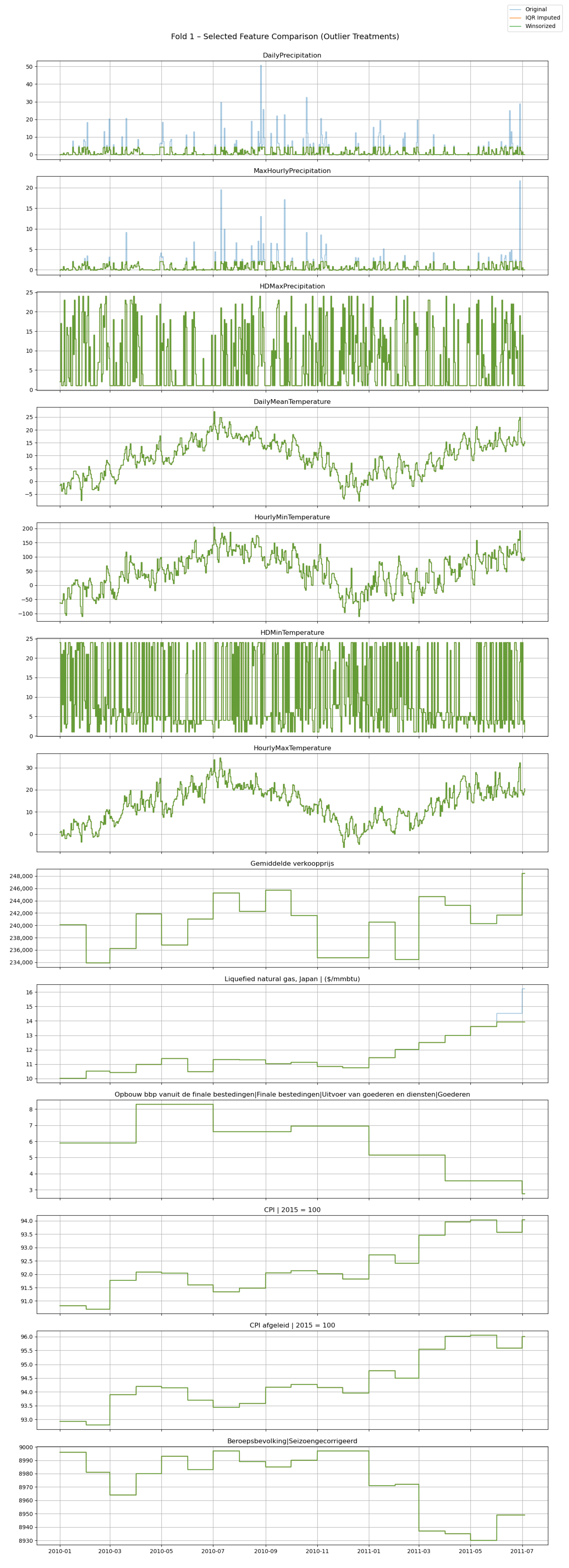
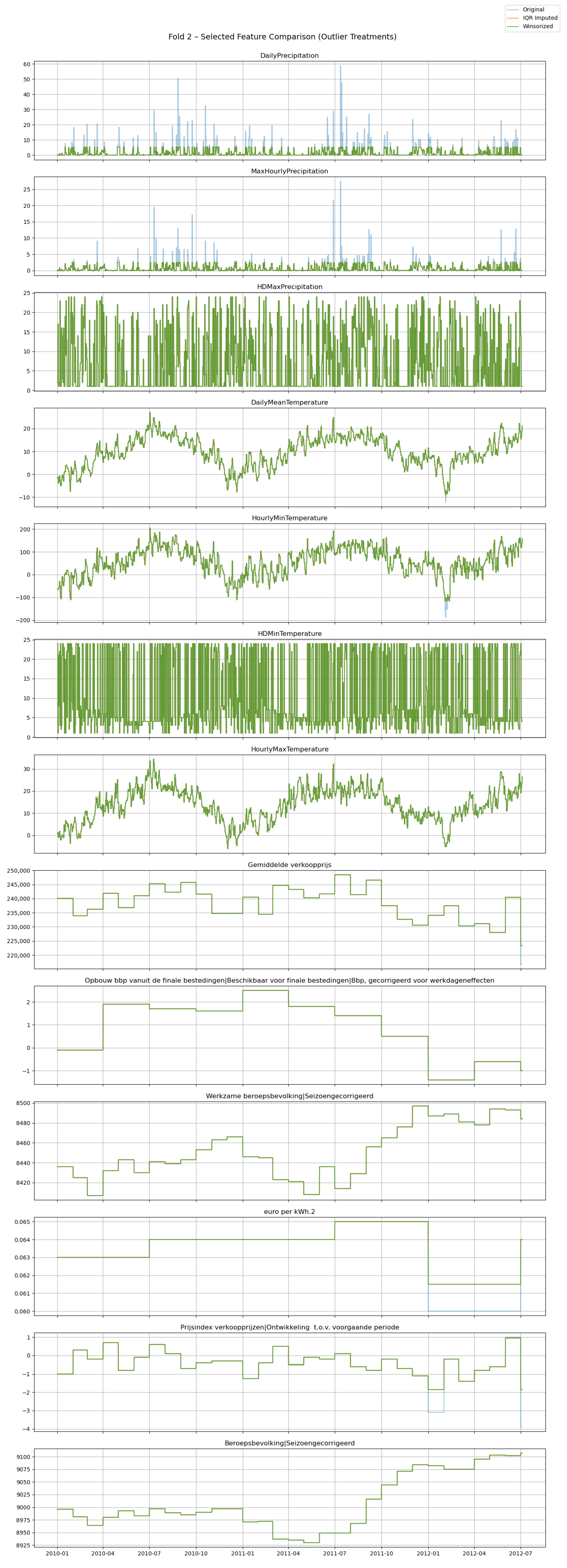
During the concluding validation pass we generated winsorisedvariants of the predictor set,
Figure A7. Visual overlays show that a handful of high-variance features exhibit smoother trajectories after clipping. Because this diagnostic was performed only after the primary analysis had been finalised, all headline results are still based on the original, non-winsorised data. The preliminary evidence nonetheless suggests that light tail-shrinking transformations merit systematic investigation in future work.
Finally, we relied on a quantum simulator. Real hardware introduces decoherence and gate errors, so observed performance may differ on physical qubits. In future work, we will explore hardware-friendly encodings and shallow circuit designs. It should also test horizons beyond 4320 h.
6. Conclusions
This study asked whether a hybrid Prophet–(Q)LSTM pipeline that integrates macroeconomic and climate predictors can improve long-horizon electricity-demand forecasting in The Netherlands. The evidence indicates that it can: relative to the classical Prophet–LSTM, the stand-alone Prophet–QLSTM achieved a mean RMSE reduction of 7.68% (2219.39 → 2048.92 MWh; mean delta 170.46 MWh) with comparable MAPE and PCC while using fewer recurrent parameters. The most substantial gains, however, came from stacking: both stacked models outperformed their non-stacked parents on all metrics, with RMSE reductions of 613.45 MWh (stacked Prophet–LSTM) and 546.51 MWh (stacked Prophet–QLSTM). Between the two stacks, performance was statistically comparable; a small PCC edge for the classical stack (p = 0.05) appears to originate from the meta-learner rather than the recurrent core.
The predictor analysis clarifies the interdependencies that drive these results. When sufficient history is available, economic signals (e.g., GDP composition, price indices, oil/gas/coal benchmarks) account for a large share of error reduction; local weather (daily/hourly temperatures and precipitation) remains consistently informative across folds. These findings, coupled with Prophet’s decomposable structure, yield forecasts that are both accurate and interpretable. In operational terms, the observed accuracy gains support more reliable seasonal planning (reserve-margin sizing, maintenance windows), increase confidence in demand-response scheduling, and strengthen procurement and hedging decisions when forecasts are paired with market price signals. Although the empirical focus is The Netherlands, the pipeline and evaluation protocol are general and can be ported to other national systems without loss of methodological validity.
To make the main answers explicit and easy to scan, we distill the findings aligned with the study questions:
SQ1 Forecast accuracy: Prophet–QLSTM improves year-round accuracy over Prophet–LSTM by 7.68% RMSE, with similar MAPE and PCC.
SQ2 Role of quantum components: Stacking dominates non-stacked variants on RMSE and MAPE; between stacks, performance is statistically comparable, with a modest PCC advantage for the classical stack (p = 0.05).
SQ3 Most relevant predictors: Economic series are pivotal when ample history is present; local weather remains a stable contributor throughout.
SQ4 Trade-offs: QLSTM attains near-parity (or better RMSE when non-stacked) with far fewer recurrent parameters, at the cost of longer training when simulated.
Overall, hybrid Prophet–(Q)LSTM architectures provide a practical path to more accurate, robust long-horizon load forecasts under climate and macroeconomic uncertainty while preserving interpretability through Prophet and strong temporal feature learning via (Q)LSTM.
Looking ahead, as error-mitigated, hardware-efficient quantum devices with higher gate fidelities become available, the wall-clock cost of QLSTM training should fall substantially, enabling more frequent re-estimation and deeper (yet shallow-depth) variational circuits; this would shift the cost–benefit balance from “accuracy at higher compute time” toward operational feasibility in real-world forecasting workflows.
Limitations and future work. QLSTM training on a simulator was slow, constraining us to a single quantum layer; future work should revisit deeper circuits on hardware-efficient backends, re-optimise feature balances for QLSTM at longer horizons (e.g., 4320 h), explore alternative meta-learners for stacking, and assess light dimensionality reduction for highly correlated predictors.
Author Contributions
Conceptualization, A.M.M.A. and S.S.M.Z.; Methodology, R.C.; Software, R.C.; Validation, R.C.; Formal analysis, R.C. and A.M.M.A.; Resources, R.C.; Data curation, R.C., A.M.M.A. and S.S.M.Z.; Writing—original draft, R.C.; Writing—review and editing, A.M.M.A. and S.S.M.Z.; Visualization, R.C.; Supervision, S.S.M.Z. and A.M.M.A.; Project administration, A.M.M.A. and S.S.M.Z. All authors have read and agreed to the published version of the manuscript.
Funding
This research received no external funding.
Institutional Review Board Statement
Not applicable.
Informed Consent Statement
Not applicable.
Data Availability Statement
Conflicts of Interest
The authors declare no conflicts of interest.
Appendix A
Appendix A.1. Formulas for Parameter Count Calculation
Appendix A.2. Model Results per Fold
Table A1.
Cross-validation results for all folds.
Table A1.
Cross-validation results for all folds.
| Fold | Baseline | Prophet–LSTM RMSE | Prophet–LSTM MAPE | Prophet–LSTM PCC | Prophet–QLSTM RMSE | Prophet–QLSTM MAPE | Prophet–QLSTM PCC | Stacked LSTM RMSE | Stacked LSTM MAPE | Stacked LSTM PCC | Stacked QLSTM RMSE | Stacked QLSTM MAPE | Stacked QLSTM PCC |
|---|
| 1 | 24.44 | 2291.87 | 15.95 | 0.58 | 2431.92 | 19.62 | 0.60 | 1745.77 | 11.19 | 0.71 | 1755.88 | 11.48 | 0.70 |
| 2 | 20.41 | 2230.42 | 45.92 | 0.38 | 1843.25 | 34.40 | 0.61 | 1885.22 | 12.50 | 0.61 | 1684.48 | 10.72 | 0.70 |
| 13 | 11.98 | 2383.14 | 13.81 | 0.14 | 1993.98 | 13.68 | 0.17 | 1562.59 | 9.22 | 0.60 | 1651.75 | 9.85 | 0.54 |
Appendix A.3. Model Comparison
Table A2.
Pairwise model comparisons (t-tests, mean deltas).
Table A2.
Pairwise model comparisons (t-tests, mean deltas).
| Metric | Model 1 | Model 2 | t-Test | p Value | Mean Delta | Winner |
|---|
| RMSE | Prophet LSTM | Prophet QLSTM | 3.12 | 0.01 | 170.46 | Prophet QLSTM |
| RMSE | Prophet LSTM | Stacked Prophet LSTM | 15.23 | 0.00 | 613.45 | Stacked Prophet LSTM |
| RMSE | Prophet LSTM | Stacked Prophet QLSTM | 10.71 | 0.00 | 546.51 | Stacked Prophet QLSTM |
| RMSE | Prophet QLSTM | Stacked Prophet LSTM | 8.95 | 0.00 | 442.99 | Stacked Prophet LSTM |
| RMSE | Prophet QLSTM | Stacked Prophet QLSTM | 10.58 | 0.00 | 376.05 | Stacked Prophet QLSTM |
| RMSE | Stacked Prophet LSTM | Stacked Prophet QLSTM | −1.88 | 0.08 | −66.94 | None |
| MAPE | Prophet LSTM | Prophet QLSTM | 1.42 | 0.18 | 1.47 | None |
| PCC | Stacked Prophet LSTM | Stacked Prophet QLSTM | 2.17 | 0.05 | −0.05 | Stacked Prophet LSTM |
Confidence Intervals per Metric, per Model
Table A3.
Comparison of RMSE between models.
Table A3.
Comparison of RMSE between models.
|
Model | Mean | Std | Shapiro Wilk | Shapiro p-Value | Normal? | CI Method | CI Lower | CI Upper |
|---|
| Prophet–LSTM | 2219.39 | 142.84 | 0.92 | 0.16 | True | t-CI | 2140.28 | 2298.49 |
| Prophet–QLSTM | 2048.92 | 156.82 | 0.91 | 0.15 | True | t-CI | 1962.08 | 2135.77 |
| Stacked Prophet–LSTM | 1605.93 | 104.07 | 0.84 | 0.01 | False | btstrp | 1560.04 | 1661.80 |
| Stacked Prophet–QLSTM | 1672.88 | 87.70 | 0.97 | 0.81 | True | t-CI | 1624.31 | 1721.44 |
Table A4.
Comparison of MAPE between models.
Table A4.
Comparison of MAPE between models.
| Model | Mean | Std | Shapiro Wilk | Shapiro p-Value | Normal? | CI Method | CI Lower | CI Upper |
|---|
| Prophet–LSTM | 17.58 | 8.17 | 0.55 | 0.00 | False | btstrp | 14.69 | 22.18 |
| Prophet–QLSTM | 16.11 | 5.48 | 0.59 | 0.00 | False | btstrp | 14.04 | 19.15 |
| Stacked Prophet–LSTM | 10.30 | 0.97 | 0.94 | 0.42 | True | t-CI | 9.76 | 10.83 |
| Stacked Prophet–QLSTM | 10.78 | 0.75 | 0.91 | 0.12 | True | t-CI | 10.37 | 11.19 |
Table A5.
Comparison of PCC between models.
Table A5.
Comparison of PCC between models.
| Model | Mean | Std | Shapiro Wilk | Shapiro p-Value | Normal? | CI Method | CI Lower | CI Upper |
|---|
| Prophet–LSTM | 0.20 | 0.29 | 0.85 | 0.02 | False | btstrp | 0.06 | 0.34 |
| Prophet–QLSTM | 0.22 | 0.26 | 0.87 | 0.03 | False | btstrp | 0.09 | 0.35 |
| Stacked Prophet–LSTM | 0.63 | 0.07 | 0.94 | 0.37 | True | t-CI | 0.59 | 0.67 |
| Stacked Prophet–QLSTM | 0.58 | 0.10 | 0.96 | 0.63 | True | t-CI | 0.52 | 0.63 |
Figure A1.
Loss progression by fold.
Figure A1.
Loss progression by fold.
Figure A2.
Target correlation heatmaps by fold (2010–2024, 4320 h).
Figure A2.
Target correlation heatmaps by fold (2010–2024, 4320 h).
Appendix A.4. Feature Histograms and Q–Q Plots
Figure A3.
Histograms and Q–Q plots of macroeconomic indicators, including GDP components, CPI metrics, and labour statistics.
Figure A3.
Histograms and Q–Q plots of macroeconomic indicators, including GDP components, CPI metrics, and labour statistics.
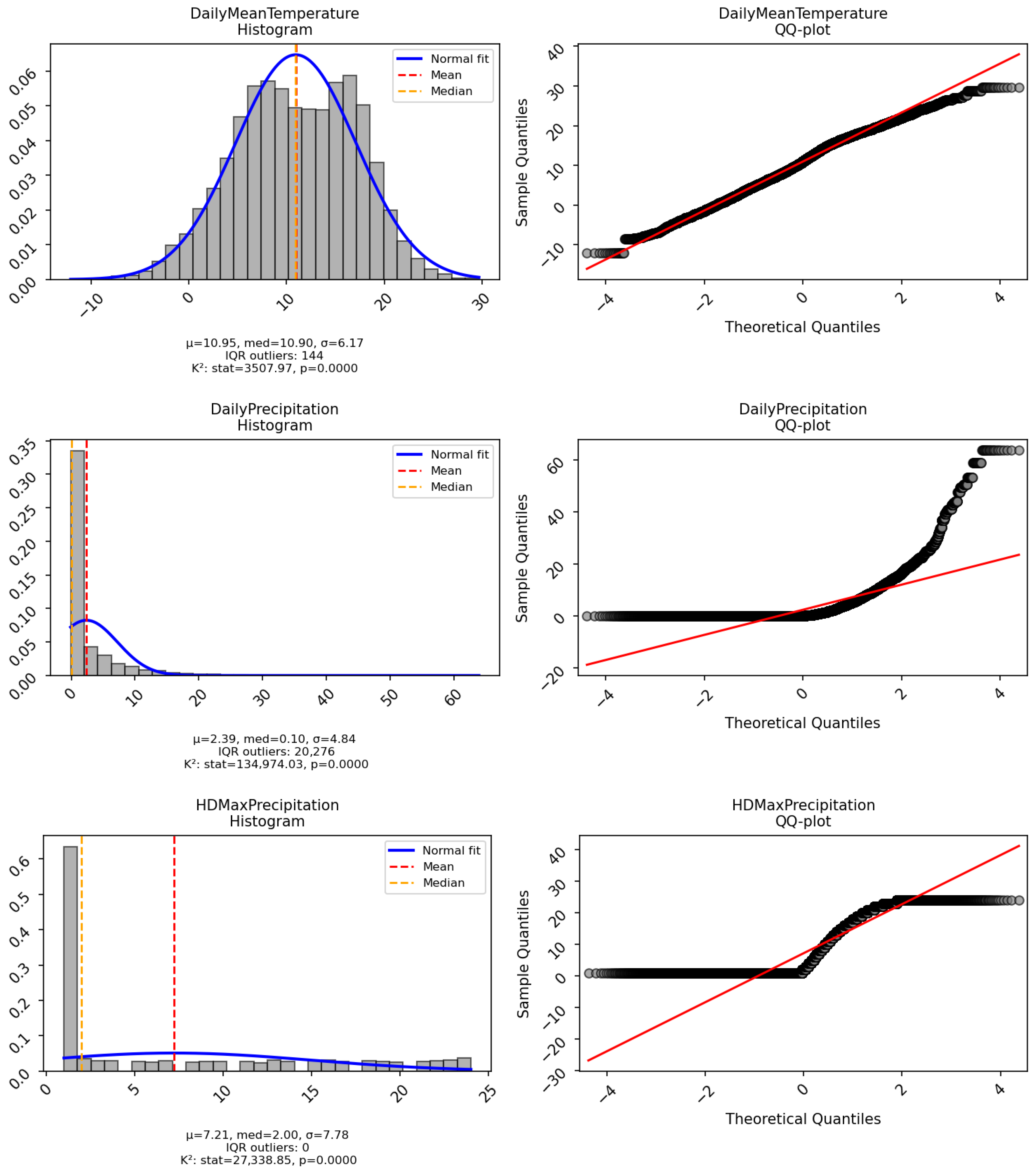
Figure A4.
Distributional plots of climate and weather variables, including daily and hourly temperature and precipitation metrics.
Figure A4.
Distributional plots of climate and weather variables, including daily and hourly temperature and precipitation metrics.
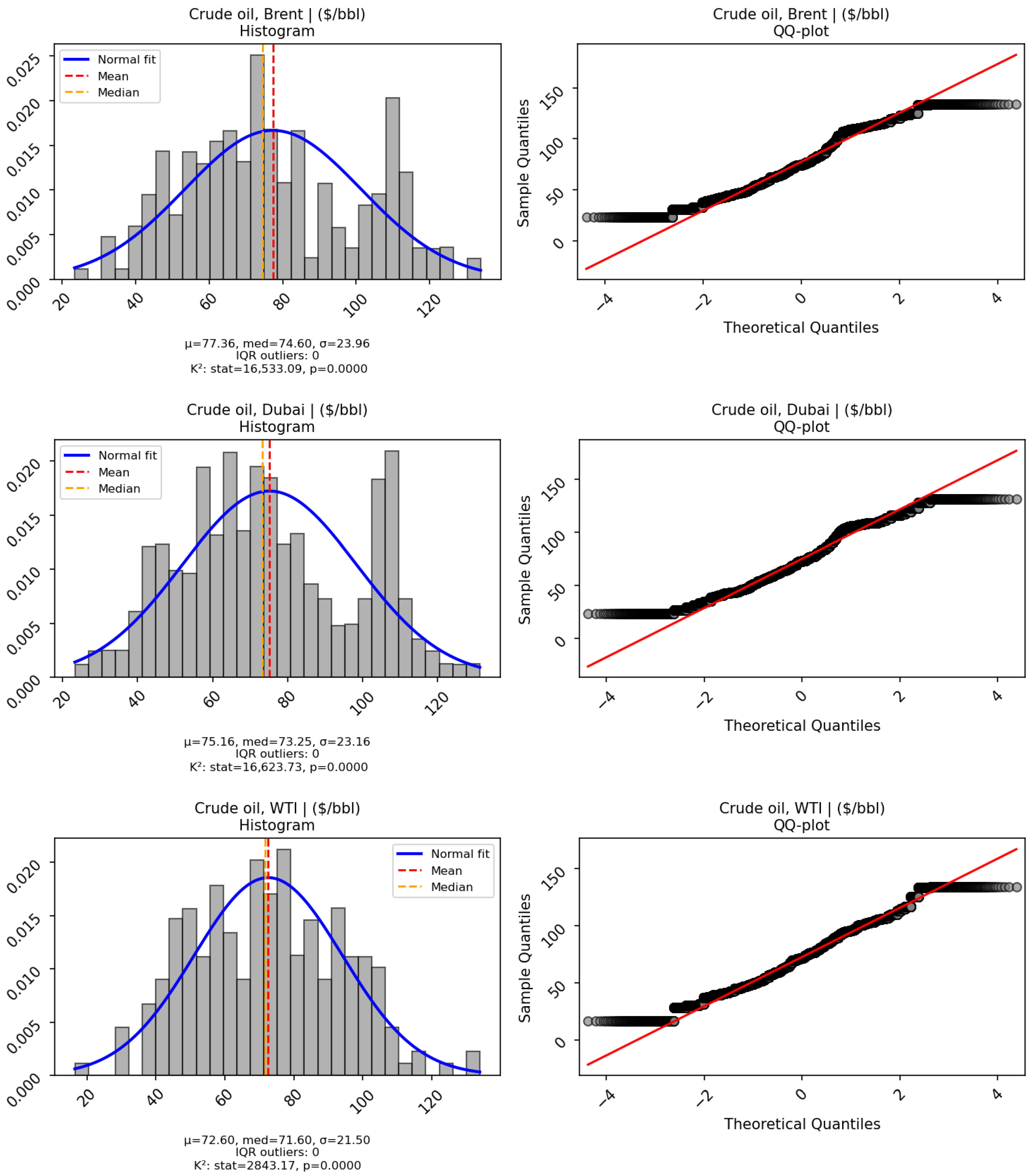
Figure A5.
Distributions of global and domestic energy and commodity prices, including oil and gas benchmarks.
Figure A5.
Distributions of global and domestic energy and commodity prices, including oil and gas benchmarks.
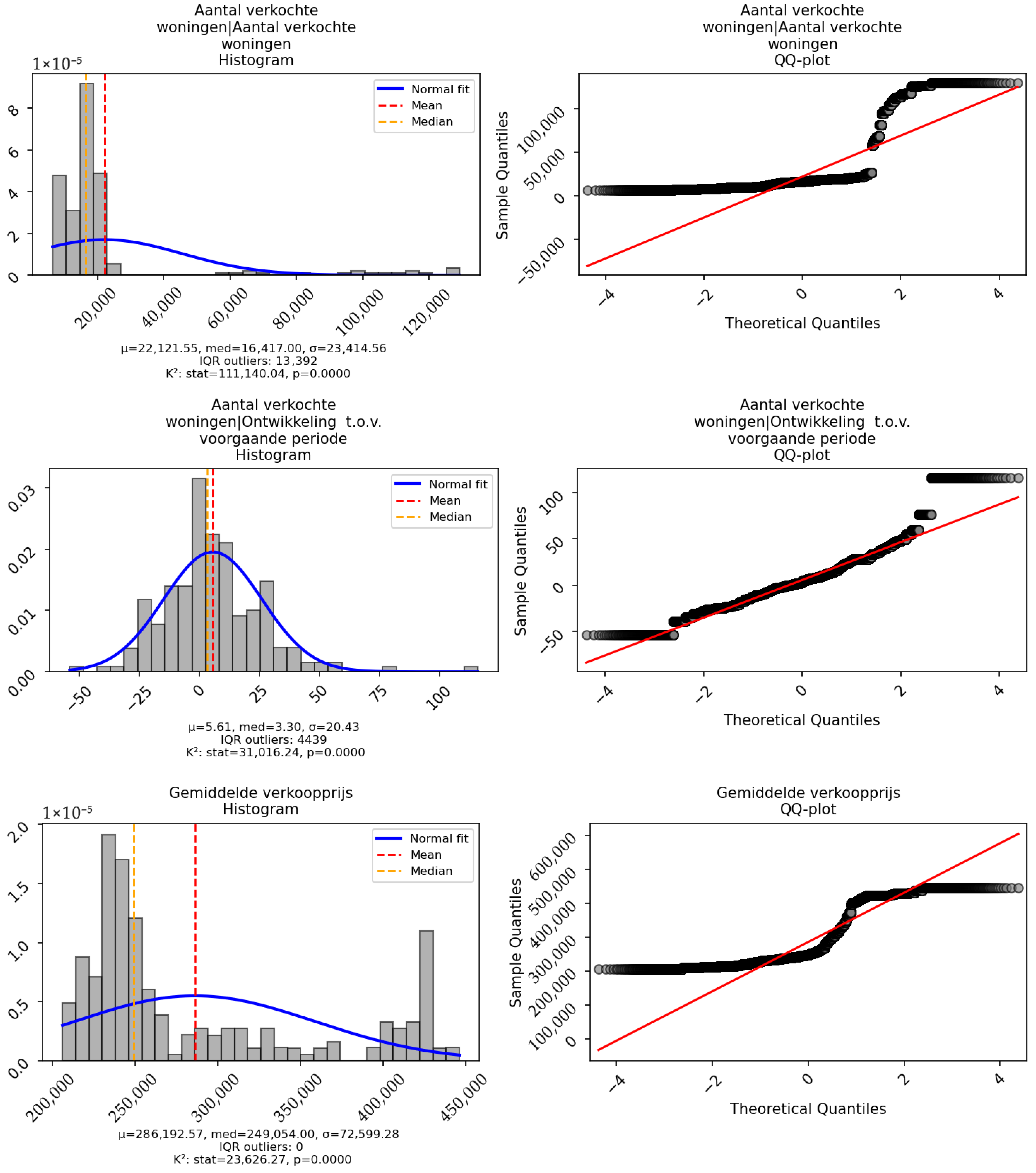
Figure A6.
Histogram and Q–Q plots of housing market variables, including sales counts and price developments.
Figure A6.
Histogram and Q–Q plots of housing market variables, including sales counts and price developments.
Appendix A.5. Winsorised Feature Distributions per Fold
Figure A7.
Winsorised predictor overlays for rolling-origin folds 1–3.
Figure A7.
Winsorised predictor overlays for rolling-origin folds 1–3.
References
- Pató, Z. Gridlock in The Netherlands; Regulatory Assistance Project: Montpelier, VT, USA, 2024. [Google Scholar]
- Banna, H.; Alam, A.; Chen, X.H.; Alam, A.W. Energy security and economic stability: The role of inflation and war. Energy Econ. 2023, 126, 106949. [Google Scholar] [CrossRef]
- Atef, S.; Eltawil, A.B. Real-time load consumption prediction and demand response scheme using deep learning in smart grids. In Proceedings of the 2019 6th International Conference on Control, Decision and Information Technologies (CoDIT), Paris, France, 23–26 April 2019; IEEE: Piscataway, NJ, USA, 2019; pp. 1043–1048. [Google Scholar]
- van de Sande, S.N.; Alsahag, A.M.; Mohammadi Ziabari, S.S. Enhancing the predictability of wintertime energy demand in The Netherlands using ensemble model Prophet–LSTM. Processes 2024, 12, 2519. [Google Scholar] [CrossRef]
- Chen, S.Y.-C.; Yoo, S.; Fang, Y.-L.L. Quantum Long Short-Term Memory. arXiv 2020, arXiv:2009.01783. [Google Scholar] [CrossRef]
- Biamonte, J.; Wittek, P.; Pancotti, N.; Rebentrost, P.; Wiebe, N.; Lloyd, S. Quantum machine learning. Nature 2017, 549, 195–202. [Google Scholar] [CrossRef] [PubMed]
- Khan, S.Z.; Muzammil, N.; Ghafoor, S.; Khan, H.; Zaidi, S.M.H.; Aljohani, A.J.; Aziz, I. Quantum long short-term memory (QLSTM) vs. classical LSTM in time series forecasting: A comparative study in solar power forecasting. Front. Phys. 2024, 12, 1439180. [Google Scholar] [CrossRef]
- Mohamed, Z.; Bodger, P. Forecasting electricity consumption in New Zealand using economic and demographic variables. Energy 2005, 30, 1833–1843. [Google Scholar] [CrossRef]
- Swan, L.G.; Ugursal, V.I. Modeling of end-use energy consumption in the residential sector: A review of modeling techniques. Renew. Sustain. Energy Rev. 2009, 13, 1819–1835. [Google Scholar] [CrossRef]
- Taylor, S.J.; Letham, B. Forecasting at scale. Am. Stat. 2018, 72, 37–45. [Google Scholar] [CrossRef]
- Sakkas, N.; Yfanti, S.; Daskalakis, C.; Barbu, E.; Domnich, M. Interpretable forecasting of energy demand in the residential sector. Energies 2021, 14, 6568. [Google Scholar] [CrossRef]
- Günay, M.E. Forecasting annual gross electricity demand by artificial neural networks using predicted values of socio-economic indicators and climatic conditions: Case of Turkey. Energy Policy 2016, 90, 92–101. [Google Scholar] [CrossRef]
- Hong, Y.-Y.; Arce, C.J.E.; Huang, T.-W. A robust hybrid classical and quantum model for short-term wind speed forecasting. IEEE Access 2023, 11, 90811–90824. [Google Scholar] [CrossRef]
- Hsu, Y.-C.; Chen, N.-Y.; Li, T.-Y.; Chen, K.-C. Quantum kernel-based long short-term memory for climate time-series forecasting. arXiv 2024, arXiv:2412.08851. [Google Scholar]
- Ravestein, P.; Van der Schrier, G.; Haarsma, R.; Scheele, R.; Van den Broek, M. Vulnerability of European intermittent renewable energy supply to climate change and climate variability. Renew. Sustain. Energy Rev. 2018, 97, 497–508. [Google Scholar] [CrossRef]
- Deser, C.; Alexander, M.A.; Xie, S.-P.; Phillips, A.S. Sea surface temperature variability: Patterns and mechanisms. Annu. Rev. Mar. Sci. 2010, 2, 115–143. [Google Scholar] [CrossRef]
- Thomas, D.N.; Dieckmann, G.S. Sea Ice: An Introduction to Its Physics, Chemistry, Biology and Geology; John Wiley & Sons: Hoboken, NJ, USA, 2008. [Google Scholar]
- Corne, D.; Dissanayake, M.; Peacock, A.; Galloway, S.; Owens, E. Accurate localized short term weather prediction for renewables planning. In Proceedings of the 2014 IEEE Symposium on Computational Intelligence Applications in Smart Grid (CIASG), Orlando, FL, USA, 9–12 December 2014; IEEE: Piscataway, NJ, USA, 2014; pp. 1–8. [Google Scholar]
- Najwa, B.N.; Hafizah, B.; Munira, I.; Abdul Razak, F. Network, correlation, and community structure of the financial sector of Bursa Malaysia before, during, and after COVID-19. Data Sci. Financ. Econ. 2024, 4, 362–387. [Google Scholar] [CrossRef]
- Sözen, A.; Arcaklioglu, E. Prediction of net energy consumption based on economic indicators (GNP and GDP) in Turkey. Energy Policy 2007, 35, 4981–4992. [Google Scholar] [CrossRef]
- Reeve, T.A.; Vigfusson, R.J. Evaluating the Forecasting Performance of Commodity Futures Prices. In International Finance Discussion Papers; Board of Governors of the Federal Reserve System: Washington, DC, USA, 2011; Volume 1025. Available online: https://www.federalreserve.gov/pubs/ifdp/2011/1025/ifdp1025.pdf (accessed on 21 September 2025). [CrossRef]
- Li, Z.; Xu, Y.; Du, Z. Valuing financial data: The case of analyst forecasts. Financ. Res. Lett. 2025, 75, 106847. [Google Scholar] [CrossRef]
- Pulicharla, M.R. Hybrid quantum–classical machine learning models: Powering the future of AI. J. Sci. Technol. 2023, 4, 40–65. [Google Scholar] [CrossRef]
- Preskill, J. Quantum computing in the NISQ era and beyond. Quantum 2018, 2, 79. [Google Scholar] [CrossRef]
- Wolpert, D.H. Stacked generalization. Neural Netw. 1992, 5, 241–259. [Google Scholar] [CrossRef]
- Resch, S.; Karpuzcu, U.R. Benchmarking quantum computers and the impact of quantum noise. ACM Comput. Surv. 2021, 54, 1–35. [Google Scholar] [CrossRef]
- Mohsen, S.; Elkaseer, A.; Scholz, S. Industry 4.0-oriented deep learning models for human activity recognition. IEEE Access 2021, 9, 150508–150521. [Google Scholar] [CrossRef]
- Di Sipio, R. rdisipio/qlstm. GitHub Repository. Available online: https://github.com/rdisipio/qlstm (accessed on 4 October 2021).
- Bergholm, V.; Izaac, J.; Schuld, M.; Gogolin, C.; Ahmed, S.; Ajith, V.; Alam, M.S.; Alonso-Linaje, G.; AkashNarayanan, B.; Asadi, A.; et al. PennyLane: Automatic differentiation of hybrid quantum–classical computations. arXiv 2018, arXiv:1811.04968. [Google Scholar]
| Disclaimer/Publisher’s Note: The statements, opinions and data contained in all publications are solely those of the individual author(s) and contributor(s) and not of MDPI and/or the editor(s). MDPI and/or the editor(s) disclaim responsibility for any injury to people or property resulting from any ideas, methods, instructions or products referred to in the content. |
© 2025 by the authors. Licensee MDPI, Basel, Switzerland. This article is an open access article distributed under the terms and conditions of the Creative Commons Attribution (CC BY) license (https://creativecommons.org/licenses/by/4.0/).

