Spatiotemporal Evolution and Multi-Scale Driving Mechanisms of Ecosystem Service Value in Wuhan, China

Abstract

This study examined the spatiotemporal dynamics and driving mechanisms of ecosystem service value (ESV) in Wuhan from 1985 to 2020. Using multi-temporal land-use data, remotely sensed vegetation indices, and socioeconomic statistics, we estimated the ESV with an improved equivalent-factor method and analyzed its drivers using a Geodetector and geographically weighted regression (GWR). Over the 35-year period, total ESV for Wuhan showed a mildly declining trend, decreasing from CNY 37.464 billion in 1985 to CNY 36.439 billion in 2020. Waterbodies contributed the largest share of ESV, followed by croplands and forests. In the urban core, ESV declined significantly, with low-value zones expanding outward from the city center. Spatial autocorrelation analysis revealed significant “high–high” and “low–low” clustering. Geodetector results indicated slope, elevation, and normalized difference vegetation index (NDVI) as the primary natural drivers, with human footprint, gross domestic product (GDP), and population density acting as important socioeconomic auxiliaries. Interactions between natural and socioeconomic factors substantially increased the explanatory power. Furthermore, GWR revealed pronounced spatial heterogeneity in the sign and magnitude of the factor effects across the study area, underscoring the complexity of ESV drivers. These findings provide quantitative evidence to support spatially differentiated ecological planning and conservation strategies during urbanization in Wuhan and the broader mid-Yangtze region.

1. Introduction

Ecosystem service value (ESV) is a key indicator for evaluating ecosystem health and its capacity to provide services to human society [1,2]. This has become a crucial research focus in the fields of ecological civilization and sustainable development. With the acceleration of urbanization, significant changes have occurred in land-use patterns, leading to the evolution of ecosystem structure and function and consequently increasing the complexity of ESV spatial patterns and trends [3,4,5,6]. As a major city in central China and the core area of the Yangtze River Economic Belt, the urban expansion of Wuhan has exerted profound effects on regional ecosystems, making it a representative case for ESV studies.

As a core metric for assessing ecosystem service functions, the ESV intuitively reflects changes in ecosystem conditions under both natural and anthropogenic influences [7]. It also serves as a fundamental basis for ecological environment evaluation and natural resource asset accounting [8,9]. The concept of “ecosystem services” was first introduced in the report The Global Impact of Human Activity on the Environment [10]. Costanza et al. [11] classified and quantified ecosystem services based on extensive research. In China, scholars such as Fu Bojie [12], Xie Gaodi [13,14,15,16], and Xiao Duning [17] have conducted specific studies on ecosystem services from the perspectives of landscape ecology, ecology, and economics. Building on the work of Costanza et al. [11], Xie Gaodi [13,14,15,16] proposed an ESV equivalent factor table tailored to the diverse terrestrial ecosystems of China and updated this methodology in 2015, forming the basis of the improved equivalent factor method. Ecosystem service value evaluation methods include the direct market and production cost methods, among which the direct market method is the most widely applied and was adopted by Costanza et al. [11]. The existing ESV research has achieved considerable maturity, including value estimation [18], spatiotemporal change [19], scenario simulation [20,21], and driving forces [22,23]. Estimations have been performed at various spatial scales, including global, national, provincial, municipal, urban agglomeration, and watershed levels [24,25,26,27,28,29,30,31], as well as for different ecosystem types such as forests and farmlands [32,33]. Studies have explored the ESV distribution and driving mechanisms based on land-use change [34,35], spatial autocorrelation [36], Geodetector [37], and geographically weighted regression (GWR) [38]. Recently, grid-scale analysis using gridded spatial units has emerged as a mainstream approach for ESV estimation and spatial pattern analysis, enabling high-resolution assessments that support the development of related fields [39].

In recent years, research on the driving forces has made significant progress, deepening our understanding of changes in ecosystem structure and function [34,40]. Analytical methods include correlation analysis [41,42], regression models [43], and Geodetector [7]. Given the spatial nonstationarity of geographic data, where attribute values vary with spatial coordinates, spatial effects must be considered in the analysis. To this end, Brunsdon et al. [44] proposed a GWR model that effectively captures local spatial heterogeneity and overcomes the limitations of global models by allowing the regression coefficients to vary by location. The use of the GWR has increased in China. For instance, Liu Jun et al. [45] used GWR and boosting regression trees to assess the spatially varying effects of tourism-related factors, such as proximity to settlements, on ESV, revealing directional spatial differences. Pan Yue et al. [46] used principal component analysis and GWR to explore the influence of natural, social, and economic factors on the greenspace ESV in the Central Yunnan Urban Agglomeration. These studies confirm the utility of GWR in accurately analyzing the driving forces behind ESV spatiotemporal variations in cities such as Wuhan.

Despite extensive research on the estimation and spatiotemporal evolution of the ESV, several gaps remain. First, most studies have focused on a single scale or employed global regression approaches without adequately revealing the multi-scale coupling of driving mechanisms and their spatial nonstationarity. Second, although regionalized modifications of equivalent value coefficients have been proposed, there is still a lack of application and uncertainty assessment in rapidly urbanizing areas, particularly in urban–water coupled zones. Third, previous studies have often examined either natural or socioeconomic factors separately, whereas few have systematically analyzed the interactions between the two and their spatial variations within urban landscapes.

Based on these research gaps, this study examined the following questions:

Research Question 1: In regions such as Wuhan, characterized by dense water networks and rapid urbanization, are spatiotemporal changes in ESV primarily driven by natural topography and vegetation?

Research Question 2: Do socioeconomic factors (e.g., GDP, population density, night-time lights, and human footprint) significantly enhance the explanatory power of ESV through interactions with topographic and vegetation variables?

Accordingly, we proposed the following hypotheses:

Hypothesis 1. 

Natural conditions (elevation, slope, and NDVI) play a dominant role in shaping the spatial differentiation of ESV; however, in areas with high concentrations of population and economic activity, the local effects of socioeconomic factors substantially alter this pattern.

Hypothesis 2. 

Strong “nonlinear enhancement” or “bivariate enhancement” interactions exist among the factors, with distinct spatial patterns between urban cores and peripheral areas.

To address these questions and test the hypotheses, this study used the Geodetector model to identify global drivers and their interactions, while incorporating the GWR model to uncover local heterogeneity, thereby establishing a multi-scale and multi-method framework for analyzing the driving mechanisms of ESV.

Therefore, this study considered Wuhan City as a case study, utilizing multi-period land-use data, remote sensing indices, and socioeconomic data, and applied the improved ESV equivalent factor method in combination with Geodetector and the GWR model to examine the spatiotemporal evolution and driving mechanisms of ESV from 1985 to 2020. This study aimed to provide theoretical support for optimizing regional ecological spatial layouts and promoting sustainable development.

2. Materials and Methods

2.1. Overview of the Study Area

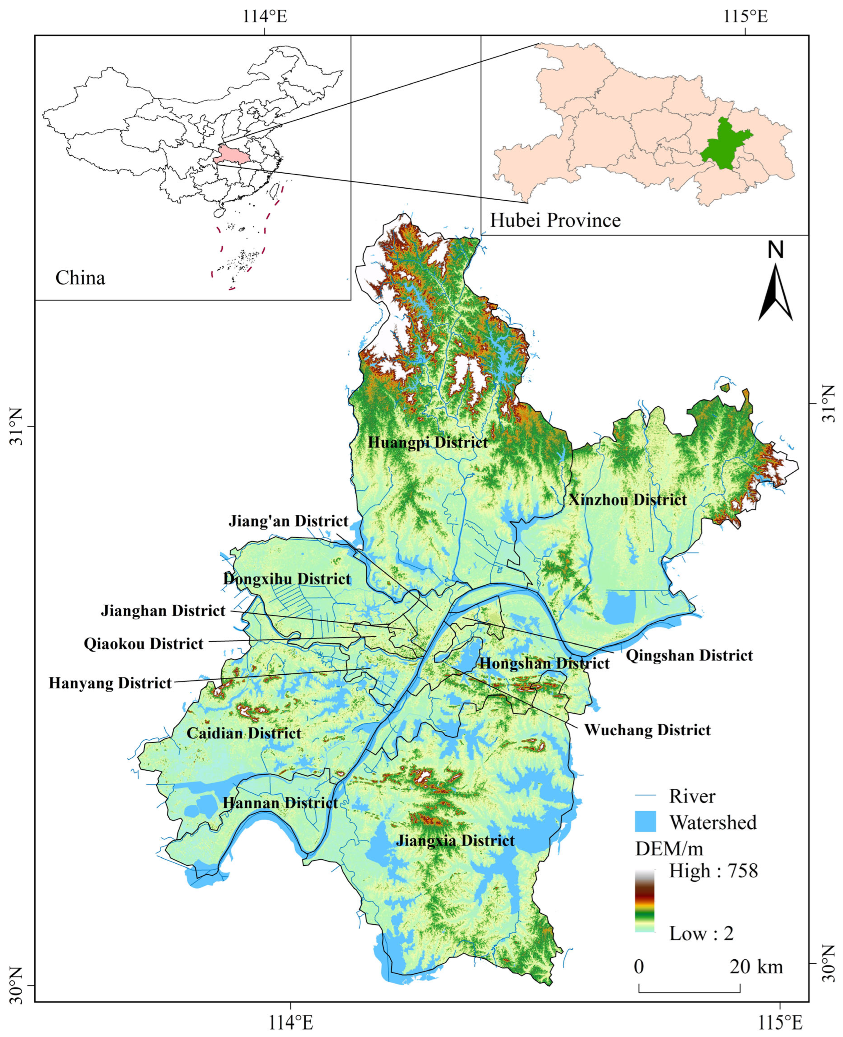
Wuhan is located at the confluence of the Yangtze and Han rivers (113°41′–115°05′ E, 29°58′–31°22′ N) and is the capital of Hubei Province. The city has a vast expanse, with a maximum horizontal distance of 134 km from east to west, maximum longitudinal distance of approximately 155 km from north to south, and a land area of 8569.15 km². Wuhan has a varied topography, dominated by low hills and plains, and its terrain is relatively gentle, with the central part being particularly flat, which provides favorable conditions for agricultural production and urban construction. Wuhan is divided into 13 administrative districts, including seven “main districts” (Jiangan, Jianghan, Qiaokou, Wuchang, Hongshan, Qingshan, and Hanyang) and six “distant districts” (Jiangxia, Caidian, Hannan, East and West Lake, Huangpi, and Xinzhou), as well as six functional districts (Figure 1). There are also six functional zones, including the Wuhan Economic and Technological Development Zone and the Wuhan East Lake New Technology Development Zone. By the end of 2022, the resident population of Wuhan is expected to reach 13.7390 million, with a population density of 1603 people/km².

2.2. Data Source

The data used in this study mainly included the administrative boundaries of Wuhan, CLCD land-use data [47], topography, rivers, transportation, meteorology, and various spatial datasets, as well as socioeconomic statistics from the Wuhan Statistical Yearbook. Detailed information on all the data is listed in

Table 1. Data sources and presentations.

Data	Abbreviation	Time	Resolution	Source
Administrative Boundaries	/	/	/	https://hubei.tianditu.gov.cn/ (accessed on 15 April 2024)
Land-use data	CLCD	1985~2020 Total 8 issues	30 m	https://zenodo.org/ (accessed on 15 April 2024)
Elevation	DEM	/	30 m	https://www.gscloud.cn/ (accessed on 15 April 2024)
Slope	Slope	/	30 m	Obtained from GIS calculations
Annual precipitation	PRE	2020	1 km	https://data.tpdc.ac.cn/ (accessed on 15 April 2024)
Average annual temperature	TEMP	2020	1 km	https://data.tpdc.ac.cn/ (accessed on 15 April 2024)
Normalized vegetation index	NDVI	2020	1 km	https://data.tpdc.ac.cn/ (accessed on 15 April 2024)
Gross domestic product	GDP	2019	1 km	https://data.tpdc.ac.cn/ (accessed on 8 May 2024)
Population density	POP	2019	1 km	https://data.tpdc.ac.cn/ (accessed on 8 May 2024)
Night-time lighting	NIL	2020	1 km	https://data.tpdc.ac.cn/ (accessed on 8 May 2024)
Human activity footprint	HFP	2020	1 km	https://data.tpdc.ac.cn/ (accessed on 8 May 2024)
Wuhan Statistical Yearbook	/	2021	/	https://tjj.wuhan.gov.cn/ (accessed on 8 May 2024)
China Rural Statistical Yearbook	/	2021	/	https://tjj.wuhan.gov.cn/ (accessed on 8 May 2024)
Cost and Benefit of National Agricultural Products	/	2021	/	https://www.stats.gov.cn/ (accessed on 8 May 2024)
Compendium of Information	/	2019	/	https://www.stats.gov.cn/ (accessed on 8 May 2024)

. All the spatial data were projected onto a unified spatial reference system (WGS_1984_UTM_Zone_50N). Data processing and analysis were conducted using ArcGIS 10.7, RStudio 2023, GWR 4.0, and GeoDa 1.14 software.

It should be noted that owing to limitations in the spatial, temporal, and spectral resolutions of remote sensing data and constraints inherent to classification algorithms, some degree of error exists in the spatial datasets used. However, the overall data accuracy was sufficiently high to satisfy the requirements of this study.

2.3. Research Methods

To systematically investigate the spatiotemporal evolution and driving mechanisms of ESV in Wuhan, this study constructed a comprehensive research framework that integrated ESV evaluation, spatial pattern analysis, identification of driving factors, and spatial heterogeneity analysis. As illustrated in the methodological flowchart (Figure 2), the analytical approach combines the improved ESV equivalent factor method, spatial autocorrelation analysis, Geodetector, and the GWR model.

2.3.1. Improved ESV Equivalent Factor Method

The equivalent factor method for ecosystem service valuation (ESV) defines the economic value of one ESV equivalent factor as the market value of the average annual grain yield per unit area in the study region (Equation (1)) [15]. Building on the revised unit-area ESV equivalent factor table developed by Xie et al. [13], and considering Wuhan’s specific conditions and relevant empirical data, this study employed a grain yield correction approach to adjust the ESV equivalent factors (

Table 2. ESV equivalent per unit area of Wuhan City in 2020.

Ecosystem Classification	Secondary Classification	Cropland	Woodland	Grassland	Waters	Unused Land	Construction Land
Supply Services	Food production	1.11	0.25	0.30	0.80	0.00	0.00
	Raw material production	0.25	0.58	0.45	0.23	0.00	0.00
	Water supply	−2.61	0.30	0.25	8.29	0.00	0.00
Regulating Services	Gas regulation	0.89	1.91	1.56	0.77	0.02	0.00
	Climate regulation	0.47	5.71	4.12	2.29	0.00	0.00
	Purification of the environment	0.14	1.67	1.36	5.55	0.10	0.00
	Hydrology	1.50	3.74	3.02	102.24	0.03	0.00
Support Services	Soil conservation	0.52	2.32	1.90	0.93	0.02	0.00
	Maintaining nutrient cycles	0.16	0.18	0.15	0.07	0.00	0.00
	Biodiversity	0.17	2.12	1.73	2.55	0.02	0.00
Cultural Services	Aesthetic landscape	0.08	0.93	0.76	1.89	0.01	0.00

).

Ecosystem services are categorized into four major types—provisioning, regulating, supporting, and cultural—covering a total of 11 specific service functions (Table 2). The equivalent factor value assigned to each service represents its relative value intensity compared with a standard equivalent factor. For example, the equivalent factor of water bodies for hydrological regulation is as high as 102.24, indicating their exceptionally high ecological value in this service. In contrast, the equivalent factor of cropland for water supply is negative (–2.61), reflecting the consumptive effect of agricultural water use on water resources.

The formula used is as follows:

$$E_a={\displaystyle \frac{1}{7}}\times {\sum }_{i=1}^j{\displaystyle \frac{m_i{p}_i{q}_i}{M}},$$

(1)

where E_a is the economic value of one ESV equivalent factor per square kilometer (CNY/km²), m_i is the sown area of grain crop i (km²), p_i is the average price of grain crop i (CNY/ton), q_i is the average yield of grain crop i per unit area (ton/km²), j is the total number of major grain crops, and M is the total sown area of all grain crops (km²).

To ensure comparability across time, a consistent valuation standard was adopted, with 2020 selected as the base year. According to statistical data, wheat, rice, and maize were Wuhan’s major grain crops in 2020. Their sown areas, yields, and market prices were obtained (

Table 3. Statistics for major grain crops of Wuhan City in 2020.

Type	Sown Area (km2)	Average Price (CNY/t)	Yield (t/km2)	Total Production (t)
Wheat	95.20	2093.00	286.28	27,254.00
Rice	1228.50	2536.47	625.27	768,512.00
Corn	170.50	2406.80	426.59	72,733.00

). Using Equation (1) together with the data in Table 3, the equivalent factor price (E_a) for Wuhan was calculated as 208,558.95 CNY/km². Combining the revised equivalent factors (Table 2) with this equivalent factor price, we derived the ESV coefficients for different land-use categories in Wuhan (

Table 4. ESV per unit area of ecosystem of Wuhan City in 2020 (unit: million CNY/km²).

Ecosystem Classification	Secondary Classification	Cropland	Woodland	Grassland	Waters	Unused Land	Construction Land
Supply Services	Food production	23.05	5.27	6.26	16.68	0.00	0
	Raw material production	5.11	12.10	9.28	4.80	0.00	0
	Water supply	−54.43	6.26	5.11	172.90	0.00	0
Regulating Services	Gas regulation	18.56	39.78	32.43	16.06	0.42	0
	Climate regulation	9.70	119.04	85.82	47.76	0.00	0
	Purification of the environment	2.82	34.88	28.36	115.75	2.09	0
	Hydrology	31.18	77.90	62.88	2132.31	0.63	0
Support Services	Soil conservation	10.85	48.44	39.52	19.40	0.42	0
	Maintaining nutrient cycles	3.23	3.70	3.02	1.46	0.00	0
	Biodiversity	3.55	44.11	35.98	53.18	0.42	0
Cultural Services	Aesthetic landscape	1.56	19.34	15.85	39.42	0.21	0
Total		55.16	410.81	324.52	2619.71	4.17	0

).

The ESV was calculated using the following formula [19]:

$$ESV={\sum }_{r=1}^{\mathrm{n}}(A_r\times V{C}_r),$$

(2)

where A_r is the area of land class r (km²) and VCr is the ESV of land class r (million CNY/km²).

2.3.2. Spatial Autocorrelation Analysis

Spatial autocorrelation analysis was used to reveal similarities between spatially adjacent data and the degree of spatial aggregation or dispersion [48]. In the present study, the global spatial autocorrelation was represented by Moran’s I index, which measures the spatial similarity of the ESV distribution across different grids in Wuhan (Equation (3)). The value of Moran’s I ranges from −1 to +1, where I > 0 indicates positive spatial autocorrelation (similar values cluster together), I < 0 indicates negative spatial autocorrelation (dissimilar values are adjacent), and I = 0 indicates no correlation (random distribution) [19]. The larger the value of I, the stronger the positive correlation.

Moran’s I is calculated as follows:

$$I={\displaystyle \frac{n{\sum }_{i=1}^n{\sum }_{j=1}^n{w}_{ij}(x_i-\overline{x})(x_j-\overline{x})}{{\sum }_{i=1}^n(x_i-\overline{x}{)}^2\left({\sum }_i{\sum }_j{w}_{ij}\right)}},$$

(3)

where x_i and x_j are the ESV values of grid cells i and $j$, respectively; $n$ is the total number of grid cells in the study area; $\overline{x}$ is the average value of ESV in the study area; and $w_{ij}$ is the spatial weight between grids $i$ and $j$, determined by the distance-based spatial weight matrix.

Local spatial autocorrelation analysis focuses on identifying the unique attributes of a variable and the correlations between adjacent variables in specific regions. The local Moran’s I index (LISA) was used to analyze whether high or low ESV values were clustered in specific grid cells, as expressed by Equation (4). Positive LISA values indicate high–high or low–low clustering, whereas negative LISA values indicate high–low or low–high clustering [49]. The LISA value was calculated as follows:

$$I_i={\displaystyle \frac{(x_i-\overline{x})}{m_0}}{\sum }_j{w}_{ij}(x_j-\overline{x}),$$

(4)

$$m_0={\sum }_i{\displaystyle \frac{(x_i-\overline{x}{)}^2}{n}},$$

(5)

where I_i is the local Moran’s I for grid cell I, x_i is the ESV value of grid cell I, $\overline{\mathrm{x}}$ is the average ESV value for the entire study area, and $w_{ij}$ is the spatial weight between grid cells i and j.

2.3.3. Geodetector

Geodetector, proposed by Wang Jinpeng et al. [50], is a statistical method used to quantify spatial differentiation and driving forces. Its core idea is to measure the similarity between the spatial distribution of explanatory factors and the phenomenon under study and assess the effect of each factor on spatial variation. Geodetector can detect the influence of individual factors as well as the interaction strength between multiple factors, including factor, interaction, risk, and ecological detection.

In this study, factor and interaction detection were applied to quantify the attribution of spatial variation in ESV in Wuhan. The process begins by dividing the study area into categories based on the values of each explanatory factor and then calculating the q-value to evaluate the explanatory power of each factor on the ESV spatial variation.

(1) Factor Detection: Factor detection reveals spatial variation in the dependent variable Y and measures the explanatory power of the independent variable X. The q-value, ranging from 0 to 1, is used to assess the significance of the influencing factors. A larger q-value indicates stronger explanatory power, whereas a smaller q-value indicates a weaker effect. The formula for calculating the q-value is as follows:

$$q=1-{\displaystyle \frac{SSW}{SST}}=1-{\displaystyle \frac{{\sum }_{h=1}^L{N}_h{\sigma }_h^2}{N{\sigma }^2}},$$

(6)

where σ is the total variance in ESV in the study area and ${\sigma }_h^2$ is the variance within each factor level h.

(2) Interaction Detection: Interaction detection identifies the combined effect of two variables and evaluates the strength of their joint contribution to ESV spatial variation. The interaction between two factors was determined by calculating the q-value for each factor alone and in combination and comparing the explanatory power of individual factors and their interactions. Interaction detection types include “double-factor enhancement,” “nonlinear enhancement,” and “independent” [51]. The interaction effect can be interpreted based on the q-value hierarchy (

Table 5. Basis for judgment of interaction explanatory power.

Basis of Judgment	Interaction Explanatory Forces Results
q(X1 ∩ X2) < Min(q(X1),q(X2))	Nonlinear attenuation
Min(q(X1),q(X2)) < q(X1 ∩ X2) < Max(q(X1),q(X2))	One-factor nonlinear attenuation
q(X1 ∩ X2) > Max(q(X1),q(X2))	Two-factor enhancement
q(X1 ∩ X2) = q(X1) + q(X2)	Independent
q(X1 ∩ X2) > q(X1) + q(X2)	Nonlinear enhancement

) [50].

2.3.4. Geographically Weighted Regression

Traditional global regression models, such as ordinary least squares (OLS), rely on the assumption of homogeneous relationships among variables. In reality, however, substantial differences in natural conditions and socioeconomic contexts across regions often cause these relationships to vary geographically, exhibiting pronounced spatial nonstationarity. Unlike traditional OLS models, geographically weighted regression (GWR) introduces spatial weights into the estimation process, allowing it to effectively capture and model spatially varying relationships and thus providing a more robust approach to nonstationarity. To explore the heterogeneous relationships between ESV and its driving factors at different spatial scales, this study introduced the GWR model. The GWR model applies spatial weighting to the regression coefficients, reflecting local variations in the relationships between variables.

The GWR model can be expressed as follows:

$$y_i={\beta }_o(u_i,v_i)+{\sum }_m{\beta }_m(u_i,v_i)x_{im}+{\epsilon }_i,$$

(7)

where $y_i$ is the dependent variable for grid cell I, (u_i, v_i) are the coordinates of grid cell I, ${\beta }_o(u_i,v_i)$ is the intercept for grid cell I, $x_{im}$ is the value of the explanatory variable m for grid cell I, ${\beta }_m(u_i,v_i)$ is the regression coefficient for the explanatory variable m at location $(u_i,v_i)$, m is the number of explanatory variables, and ${\epsilon }_i$ is the random disturbance term.

Additionally, to improve the model fitting accuracy, this study used the adaptive bi-square kernel function and estimated the parameters and regression coefficients using the GWR4 software.

The GWR model significantly improves the fit compared to that with the global regression model, as indicated by a reduction in the residual sum of squares, and yields a higher R² value. This enhances the ability of the model to explain the spatial relationships between the driving factors and ESV.

3. Results and Analysis

3.1. Time Characteristics of Land-Use Change in Wuhan

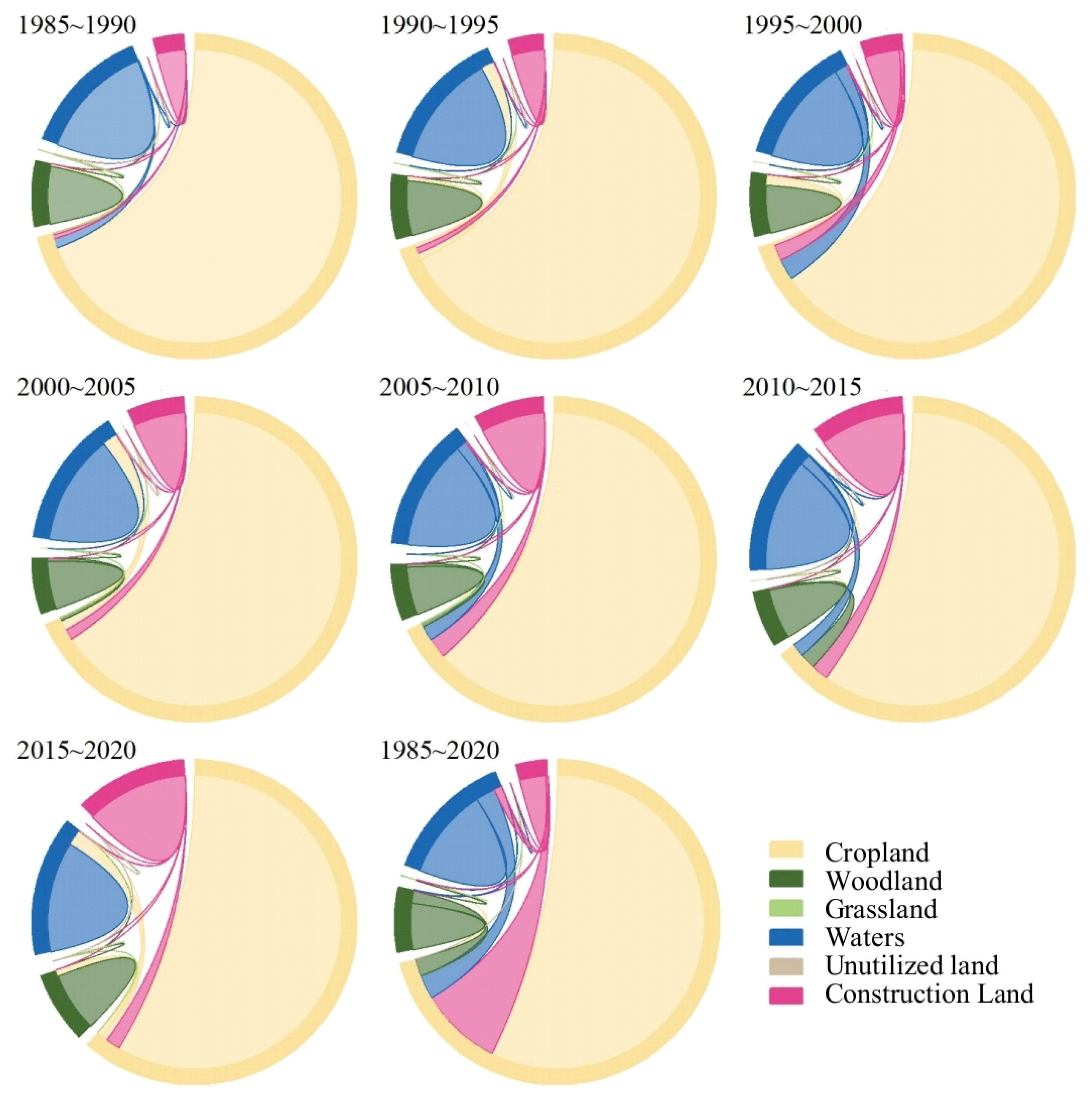
The land-use structures of Wuhan City from 1985 to 2020 are listed in

Table 6. Land-use structure of Wuhan City in 1985~2020 (unit: km²).

Land-Use Type	Year
	1985	1990	1995	2000	2005	2010	2015	2020
Cropland	6482.12	6366.39	6390.18	6257.51	6199.37	5948.03	5615.63	5580.08
Woodland	602.01	596.18	588.83	514.94	516.39	522.22	661.00	652.25
Grassland	12.85	11.19	5.49	3.07	3.90	3.99	1.86	1.25
Water	1197.58	1283.11	1207.94	1281.94	1219.73	1250.50	1277.22	1171.03
Construction Land	289.22	326.88	391.58	526.90	645.26	860.45	1029.53	1180.45
Unutilized Land	1.64	1.67	1.40	1.07	0.76	0.23	0.19	0.36

. The land-use transfer matrix is presented in

Table 7. Land-use transfer matrix of Wuhan City in 1985~2020 (unit: km²).

Year		2020
		Cropland	Woodland	Grassland	Water	Construction Land	Unused Land	Total
1985	Cropland	5238.33	177.12	0.99	241.71	823.66	0.31	6482.12
	Woodland	120.68	465.63	0.15	4.24	11.31	0.00	602.01
	Grassland	3.34	6.32	0.07	1.61	1.51	0.00	12.85
	Water	197.14	2.36	0.03	917.62	80.39	0.05	1197.58
	Construction Land	20.29	0.82	0.00	4.86	263.24	0.00	289.22
	Unused Land	0.31	0.00	0.00	0.99	0.34	0.00	1.64
	Total	5580.08	652.25	1.25	1171.03	1180.45	0.36	8585.42

, and the land-use transition chord diagram is shown in Figure 3.

As evident in the tables, during the 35 years, the areas of all land types in Wuhan underwent varying degrees of change. Cultivated land was the predominant land type throughout the study period. Its area accounted for 75.50%, 74.15%, 74.43%, 72.89%, 72.21%, 69.28%, 65.41%, and 64.99% of the total area in 1985, 1990, 1995, 2000, 2005, 2010, 2015, and 2020, respectively. Although the area of cultivated land was the largest, its total area showed a continuously decreasing trend, with a cumulative decrease of 902.04 km² over the 35-year period. The largest decrease occurred between 2005 and 2010, followed by 1995–2000 and 2010–2015. With accelerating urbanization, the pressure to convert land for built-up use has increased. Concurrent rural-to-urban labor migration and population decline have reduced the area available for agriculture, thereby contracting cultivated land. Environmental pollution and soil degradation undermine both the quantity and quality of arable land, making some plots unsuitable for cultivation. In addition, policy directions, such as land use planning, farmland protection measures, and urban expansion policies, have significantly influenced the amount and spatial composition of cultivated land. Collectively, these processes have reshaped the quantity, quality, and spatial structure of croplands.

In contrast, waterbodies maintained relatively stable areas, accounting for 13.95%, 14.95%, 14.07%, 14.93%, 14.21%, 14.57%, 14.88%, and 13.64% of the total area in the corresponding years. Croplands and built-up land represent the primary sinks for waterbody loss, with the period of 1995–2000 exhibiting the largest area of conversion from water to cropland. Changes in waterbodies are influenced not only by land-use change but also by urban planning and ecological protection policies. During urban development, Wuhan implemented measures to protect important aquatic systems and limit excessive reclamation to safeguard ecological function and sustainable water use. In addition, climatic and hydrological conditions, such as precipitation regimes and water-resource management policies, also affect temporal and spatial variations in the extent of waterbodies.

Built-up land and forest land areas were relatively small, with average proportions of 7.64% and 6.78%, respectively, across the eight time periods. The built-up land area increased the most, growing by 891.23 km², whereas forest land showed an initial decrease and then an increasing trend, with a net increase of 50.24 km². Grassland and unused land accounted for a small proportion, averaging 0.06% and 0.01%, respectively.

3.2. Time Evolution Characteristics of ESV

Based on the ESV equivalent factor coefficients for Wuhan in 2020 (

Table 8. ESV of each land-use type of Wuhan City from 1985–2020 (unit: CNY 100 million).

Land-Use Type	Year
	1985	1990	1995	2000	2005	2010	2015	2020
Cropland	35.76	35.12	35.25	34.52	34.20	32.81	30.98	30.78
Woodland	24.73	24.49	24.19	21.15	21.21	21.45	27.15	26.79
Grassland	0.42	0.36	0.18	0.10	0.13	0.13	0.06	0.04
Water	313.73	336.14	316.45	335.83	319.53	327.59	334.59	306.78
Unutilized Land	0.0007	0.0007	0.0006	0.0004	0.0003	0.0001	0.0001	0.0002
Construction Land	0.00	0.00	0.00	0.00	0.00	0.00	0.00	0.00
Total	374.64	396.11	376.07	391.60	375.07	381.99	392.79	364.39

), the total ESV of different land-use types in Wuhan from 1985 to 2020 was estimated using Equation (2). The results are summarized in Table 8.

Overall, the total ESV in Wuhan fluctuated within a relatively stable range, with an average value of CNY 38.158 billion across the eight time periods. The highest ESV value occurred in 1990, at CNY 39.611 billion, and the lowest was in 2020, at CNY 36.439 billion. Over the 35-year period, the total ESV of Wuhan decreased by approximately CNY 1.024 billion. The contribution of different land-use types to ESV varied over time, with waterbodies consistently contributing the most, accounting for over CNY 30 billion in ESV in each period, averaging 84.85% of the total ESV. This is owing to the significant hydrological regulation function of waterbodies as well as the dense water network and large water area of Wuhan, which provide substantial ESV. During this period, the total ESV from the waterbodies decreased by approximately CNY 1.95 billion.

Following waterbodies, cultivated and forest lands contributed the most, with average ESV values of CNY 3.368 billion and CNY 2.390 billion, respectively. Cultivated land ESV consistently decreased, with a decrease of CNY 0.498 billion, whereas forest land ESV showed a trend of “decrease first, then increase,” with an overall increase of CNY 0.206 billion. The contributions of grassland and unused land to the ESV were relatively small, accounting for less than 1% of the total value. This is because of their limited area and low utilization rate. The main contributors to the ESV of Wuhan were waterbodies, cultivated land, and forest land.

From a temporal perspective, the decreases in ESV in waterbodies and cultivated land and in the overall ESV reflect the decline in the environmental quality of Wuhan. This trend is largely driven by the expansion of built-up land, which leads to a reduction in valuable ecosystems such as waterbodies and cultivated land, resulting in a decrease in ESV. Despite the overall decrease, waterbodies, as a critical component of high-value areas, play an essential role in maintaining the ESV in the city.

Table 9. Contribution of various ecosystem service functions to ESV in Wuhan from 1985 to 2020 (%).

Year	Provisioning Services	Regulating Services	Supporting Services	Cultural Services
1985	2.05%	92.40%	3.70%	1.85%
1990	2.43%	92.15%	3.59%	1.82%
1995	2.15%	92.35%	3.66%	1.84%
2000	2.47%	92.22%	3.51%	1.80%
2005	2.30%	92.32%	3.56%	1.81%
2010	2.59%	92.10%	3.51%	1.80%
2015	2.96%	91.65%	3.56%	1.83%
2020	2.64%	91.85%	3.66%	1.85%

shows that between 1985 and 2020 the contribution pattern of service categories to total ESV in Wuhan remained relatively stable. Regulating services dominated throughout, accounting for more than 91% of total ESV; supporting services ranked second, remaining between 3.51% and 3.70%; provisioning services contributed relatively little, ranging from 2.05% to 2.96%; and cultural services contributed the least, between 1.80% and 1.85%. Overall, the ESV composition in Wuhan is centered on regulating services, with the combined contribution of the other three categories (provisioning, supporting, and cultural) totaling less than 10%. This pattern is primarily attributable to the extensive waterbodies of the city and the important role of aquatic ecosystems in climate and hydrological regulation; the ESV equivalent coefficient for regulating services is the highest, at 2312.

3.3. Spatial Evolution Characteristics of ESV

3.3.1. Spatial Distribution of Total ESV

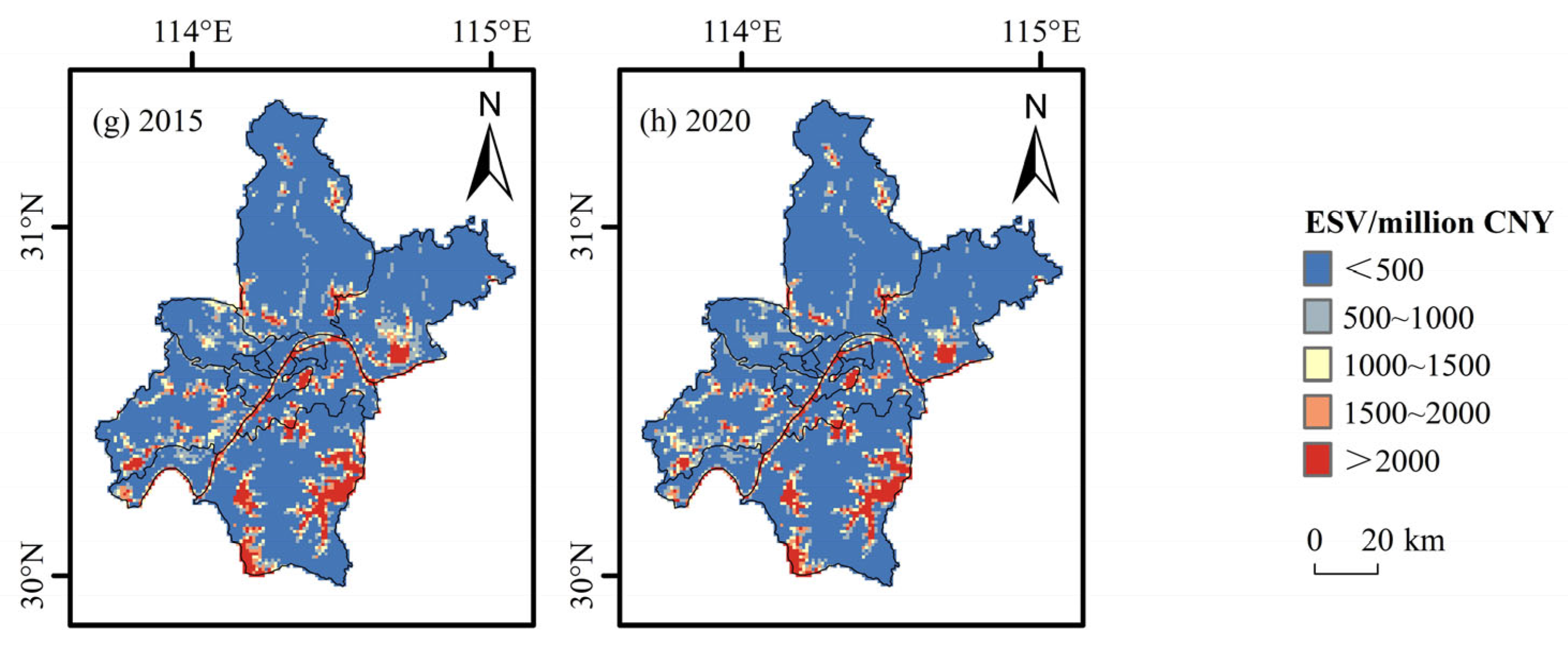
The spatial distribution of ESV in Wuhan from 1985 to 2020 is shown in Figure 4. The spatial distribution analysis showed that the overall distribution of ESV in Wuhan remained stable for over 35 years. However, significant changes were observed in the central urban area where the ESV decreased substantially. High-value grids, where the ESV exceeded CNY 20 million, were concentrated around waterbodies, particularly in districts such as Jiangxia, Hongshan, Wuchang, and Caidian, as well as in areas near the Yangtze and Han rivers. Although the ESV of built-up land was not considered in this analysis, its high spatial concentration in the central urban area of Wuhan helped maintain relatively high total ESV values in these regions. Conversely, areas farther from waterbodies had lower ESV values. As the city expanded outward, cultivated land and waterbodies were gradually replaced by built-up land, resulting in a decrease in ESV. This trend is evident in the significant increase in low-value regions, particularly in areas with ESV less than CNY 5 million, which are primarily located on the outskirts of the city in cultivated land areas.

Thus, the spatial distribution of ESV in Wuhan remained stable over time, but the ESV in the central urban area decreased significantly. This reflects the tradeoff between urban development and ecological conservation. Waterbodies are crucial for maintaining a high ESV, whereas the extensive spread of built-up land in the central urban area helped sustain the high ESV values in these regions. In contrast, areas distant from waterbodies, particularly cultivated land areas, exhibited lower ESV, with low-value zones expanding significantly as urbanization proceeded. These results underscore the need for effective ecological protection measures to balance economic development and environmental preservation during urbanization.

3.3.2. Spatial Distribution of Changes in ESV

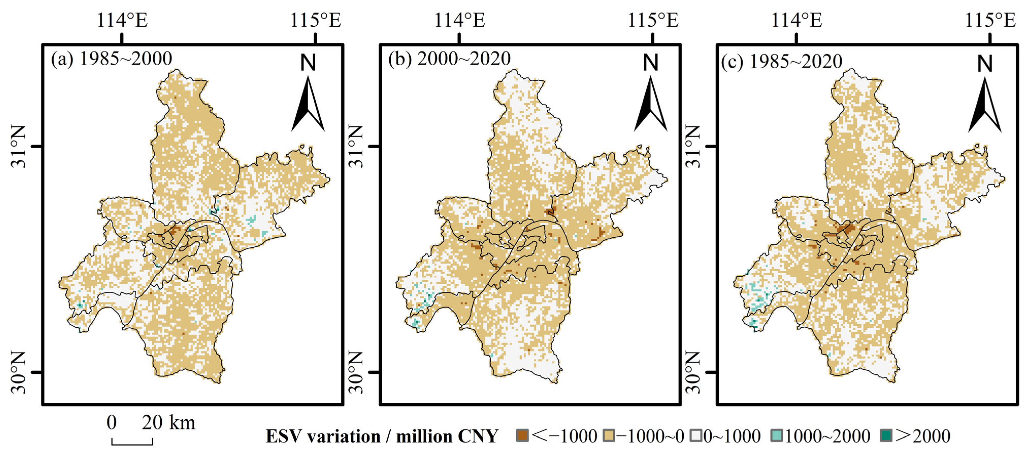
Based on the ESV data from 1985, 2000, and 2020, the spatial distribution of changes in ESV between 1985 and 2020 was analyzed, and the results are shown in Figure 5.

Between 1985 and 2020, the changes in ESV ranged from CNY −1000 to 0 million and from CNY 0 to 1000 million, with the largest area in the central region. The areas with negative ESV change (CNY −1000 to 0 million) were primarily concentrated in the central urban area, whereas the areas with positive ESV change (CNY 0 to 1000 million) were mainly distributed in the peripheral regions of the city, such as the southwestern part of Caidian and the southeastern part of Huangpi. This indicates that, during this period, some regions of Wuhan experienced improvements in habitat conditions and ecological protection. The areas with the most significant reductions in ESV were in the east of Dongxihu, west of Jiangan, north of Qiaokou, and north of Wuchang. These regions are the main areas of urban expansion, further emphasizing the negative impact of urbanization on the ESV. The regions with the largest increases in ESV were located in Caidian and Hannan, where land-use changes were mainly owing to the transformation of land into waterbodies and cultivated land, leading to a noticeable increase in ESV.

Overall, the areas of ESV increase were smaller than those of decrease, and the total area of decreased ESV has been expanding continuously over the 35 years. The expansion of built-up land has contributed to a continuous increase in the ESV reduction areas, highlighting the ongoing deterioration in habitat quality. This indicates that the ecological protection efforts in Wuhan must be intensified in the face of rapid urban development.

3.3.3. Global Spatial Autocorrelation

The global Moran’s I index was calculated to analyze the overall spatial pattern of ESV distribution in Wuhan from 1985 to 2020. The results are shown in

Table 10. Moran’s I of ESV in Wuhan City from 1985 to 2020.

Year	1985	1990	1995	2000	2005	2010	2015	2020
I	0.70	0.71	0.70	0.71	0.71	0.70	0.71	0.70
Z-Score	93.20	93.57	93.41	94.61	93.63	93.43	93.92	92.78
p-value	0.00	0.00	0.00	0.00	0.00	0.00	0.00	0.00

.

The global Moran’s I index for ESV in Wuhan during the 35-year period consistently remained around 0.70, with Z-scores greater than 2.58 for all years, indicating that the likelihood of this clustering pattern occurring randomly is less than 1%. This shows a strong positive spatial autocorrelation, indicating that areas with high ESV values are adjacent to other areas with high ESV values, and similarly for low ESV areas. This suggests that high-value ESV regions are clustered around water-dense areas, whereas low-value ESV regions are scattered across urban expansion zones.

The global Moran’s I index and its associated measures remained relatively stable over the 35-year period with no significant decrease or increase in clustering intensity. This stability reflects the overall ESV distribution in Wuhan, which remains consistent despite urban development. As urbanization progressed, the overall clustering of ESV remained intact, further emphasizing the need to balance urban growth and ecological preservation.

3.3.4. Local Spatial Autocorrelation

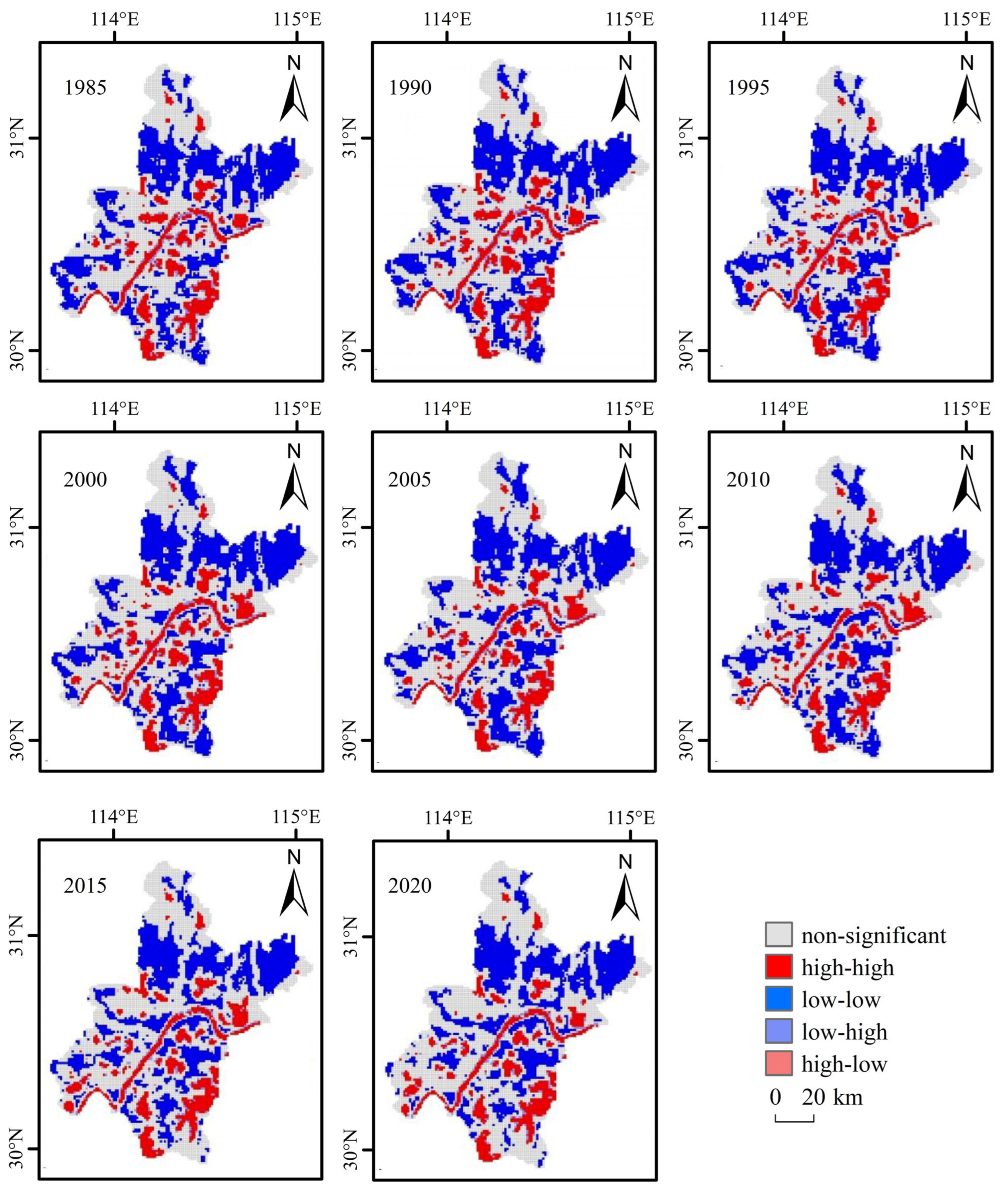
The local Moran’s I index (LISA) was calculated using GeoDa software to further analyze the local spatial autocorrelation of the ESV in Wuhan from 1985 to 2020. The results are shown in Figure 6.

The LISA clustering map indicates that ESV in Wuhan exhibits strong “high–high” and “low–low” clustering patterns at each stage, with the spatial distribution remaining largely consistent over time. The “high–high” clusters, which represent regions with high ESV values, are mainly concentrated in water-rich areas, such as Jiangxia District, along the Yangtze River and Han River. These areas show a distinct tendency to form band- or cluster-shaped distributions, although some fragmentation has occurred over time. In contrast, “low–low” clusters, which indicate regions with low ESV values, are widespread and are mainly located in areas such as Huangpi District and the northern part of Xinzhou District. These regions reflect the negative impacts of urbanization, with increasing built-up land and the loss of valuable ecosystems such as cultivated land and waterbodies.

The LISA clustering analysis also showed that “low–low” regions expanded significantly in the outer parts of the urban area. Notably, areas like the southern part of Jiangxia District, which was a “low–low” cluster in 2000, had largely transitioned to “not significant” regions by 2020. Conversely, the areas surrounding the main urban area, where built-up land had widely expanded, predominantly exhibited “low–low” and insignificant clustering patterns.

This spatial distribution analysis further confirms that the ESV in Wuhan is highly concentrated in water-dense areas, and urbanization continues to lead to the expansion of low-value ESV zones. This calls for a more effective approach to urban planning and ecological protection, in which natural ecosystems are prioritized for conservation, especially in rapidly urbanizing areas.

4. Driving Force Analysis

4.1. Factor Detection and Interaction Analysis

Nine driving factors, including natural geographic (elevation, slope, precipitation, temperature, and NDVI) and socioeconomic (GDP, population density, night-time light intensity, and human activity footprint) factors, were selected for analysis. Considering that Geodetector requires categorical variables, optimal discretization methods were applied to divide each factor into appropriate categories based on quantiles, geometric intervals, and natural breaks.

The factor detection results (Figure 7) showed that all factors had significant explanatory power for the spatial variation in ESV (p < 0.01). Among the natural factors, slope (q = 0.78) and elevation (q = 0.67) were the main drivers, whereas the explanatory powers of the NDVI, human activity footprint, GDP, and population density were weaker. Overall, natural factors have higher average q-values than socioeconomic factors, indicating that the ESV distribution is primarily driven by natural terrain and vegetation patterns.

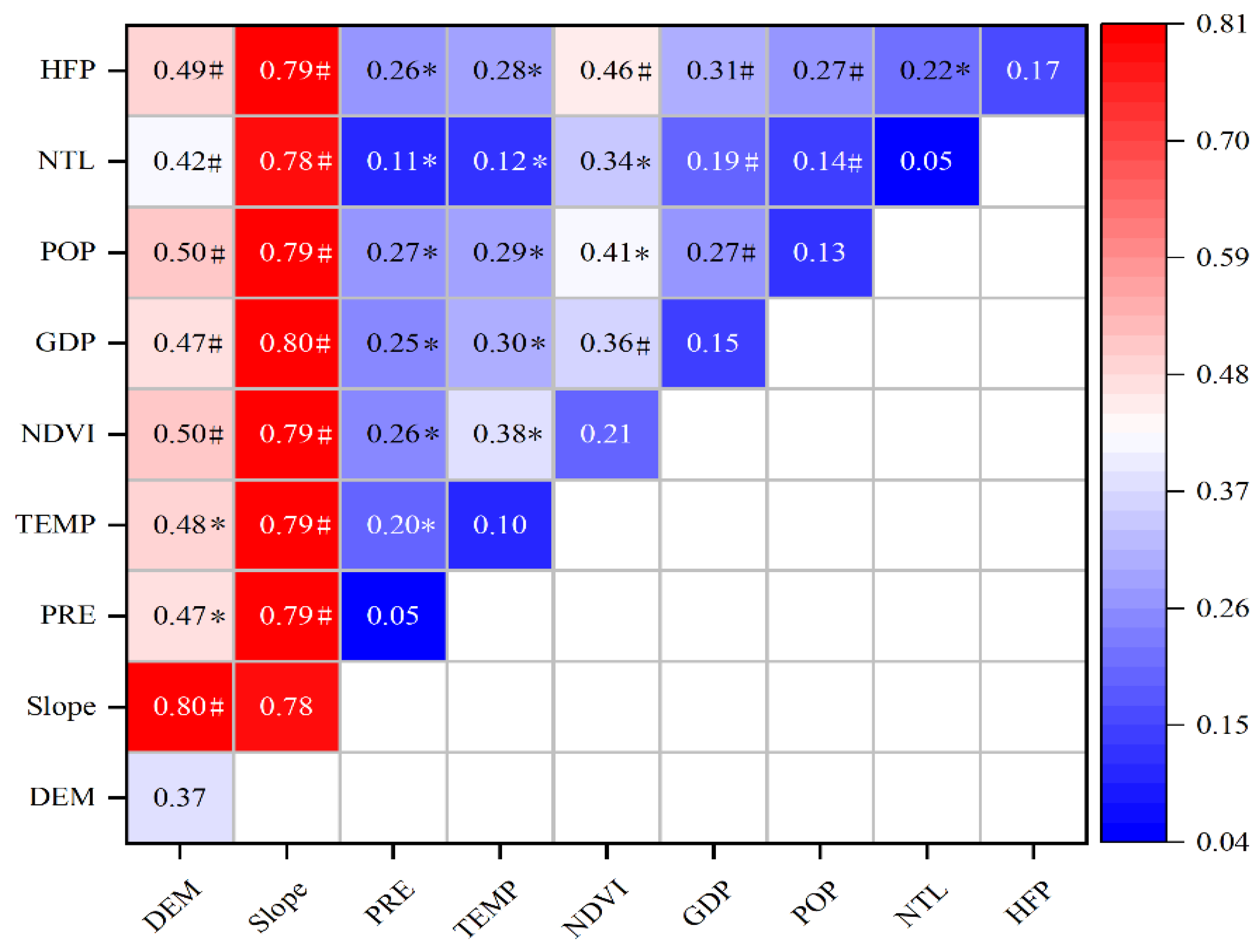
The results of the interaction analysis (Figure 8) demonstrate that the combined explanatory power of any two factors exceeds that of each individual factor. The interaction types are predominantly characterized as “bivariate enhancement” and “nonlinear enhancement,” indicating that the spatial distribution of ESV is driven by the synergistic effects of multiple factors. Notably, interactions such as “slope ∩ GDP” (q = 0.80), “slope ∩ human footprint” (q = 0.79), and “elevation ∩ slope” (q = 0.80) contribute significantly to the spatial variation of ESV. These findings suggest that the coupled interactions between natural and socioeconomic factors constitute a core mechanism shaping the spatial patterns of ESV in Wuhan. High q-value interactions imply that topographic conditions (e.g., DEM, slope) not only directly govern the provision of ecosystem services by influencing soil, hydrology, and vegetation growth but also modulate how human activities impact ecosystems in space. For example, in steep areas, land use and economic activities more readily trigger soil erosion and vegetation degradation, thereby increasing the joint explanatory power of “slope × GDP/human footprint.” The coupling of elevation and slope likely reflects combined effects of vertical zonation in biomass and constraints on land use that jointly shape service provision.

4.2. Geographically Weighted Regression (GWR)

In this study, the GWR model was implemented using GWR4 software to examine the spatial relationships between ESV and various driving factors in 2020. The model employed a Gaussian kernel function and an adaptive bi-square weighting scheme with the optimal bandwidth determined by the corrected Akaike information criterion (AICc). The results indicate that the GWR model significantly improved model performance, with a residual sum of squares of 4.15 × 10⁸, substantially lower than that of the global ordinary least squares model (residual sum of squares = 1.91 × 10⁹). The coefficient of determination (R²) increased from 0.49 to 0.89, suggesting that the GWR model provided a more robust explanation for spatial heterogeneity in the relationship between ESV and its drivers.

The spatial distribution of GWR regression coefficients (Figure 9) indicates marked spatial heterogeneity in the effects of different drivers on ESV in Wuhan. Overall, clear contrasts emerged between the spatial patterns of the natural environmental and socioeconomic factors.

Topographic factors (elevation and slope) exhibited positive coefficients in the outer hilly and mountainous margins (Figure 9a,b), indicating that greater elevations and steeper slopes tended to enhance the ESV in areas with pronounced relief. In contrast, the coefficients were negative in the low-lying plains and river–lake-dense regions within the urban area, suggesting a limited or adverse role of topography for ESV in highly urbanized landscapes.

The climatic drivers (precipitation and temperature) showed large spatial variability in their coefficients (Figure 9c,d). Positive effects occurred in some upstream and ecologically sensitive zones, implying that improved hydrothermal conditions promote ESV. However, negative coefficients were found in central urban areas and parts of the surrounding region, indicating that climate variables may be coupled with adverse urban processes (e.g., flooding and urban heat island effects) under intensive urbanization.

The vegetation index (NDVI) was strongly and positively associated with ESV across most suburban and natural ecological areas (Figure 9e), indicating that higher vegetation cover generally strengthens ecosystem service provision. However, in the urban core, the positive effect of NDVI weakened or even reversed, likely owing to greenspace fragmentation and anthropogenic modification.

Socioeconomic factors (GDP, population density, night-time lights, and human footprint) generally showed significantly negative coefficients in urban areas (Figure 9f–i), particularly in industrial, commercial, and densely populated districts, indicating that intensified human activities strongly suppress ESV. In a few peri-urban or ecologically and economically coupled zones, some socioeconomic coefficients are weakly positive or neutral, suggesting that, under specific conditions, economic activity can coexist with or even support ecological protection.

5. Discussion and Conclusions

5.1. Discussion

This study systematically explored the spatiotemporal evolution and driving mechanisms of ESV in Wuhan from 1985 to 2020. Compared with the existing literature, the key innovations and findings of this study are detailed below.

(1) Regionalized ESV coefficients adjusted to local grain yield. We developed and applied locally adjusted equivalent factors based on regional grain yields to improve the contextual suitability of the ESV estimates for Wuhan. Although the citywide ESV total showed limited fluctuation over the 35-year period, cultivated land area continuously declined, whereas built-up land expanded markedly; in particular, ESV in the urban core exhibited a clear downward trend. These results indicate that rapid urbanization exerts a substantial disturbance on ecosystem service provision and confirm the feasibility of regionalized equivalent factors for tracking changes in ESV during urban expansion.

(2) Complementary use of Geodetector and GWR. Geodetector was used to identify dominant drivers and interaction types (e.g., “slope ∩ GDP” and “slope ∩ human footprint,” showing bivariate or nonlinear enhancement), whereas GWR revealed the local heterogeneity and the spatial distribution of positive and negative effects. The combined use of these two methods strengthens the explanatory power of the driving mechanisms and provides richer spatial details.

(3) Natural base-dominated socioeconomic factors are amplified via interactions. Under rapid urbanization, we quantitatively confirmed a mechanism in which natural drivers play a leading role, whereas socioeconomic drivers act as important auxiliaries whose interactions significantly increase the explanatory power. In water-network-dense urban areas, such as Wuhan, waterbodies and topography decisively influence ESV, whereas socioeconomic pressures can locally alter ESV spatial patterns, especially in the urban core and its expansion zones. Integrate an ESV-guided zoning regime into urban planning by using Geodetector and GWR outputs (e.g., high-q hotspots such as slope × GDP and slope×human footprint) to delineate conservation-priority, development-restriction, and controlled-development zones. In conservation zones, prohibit land-use conversion and high-intensity development and prioritize restoration of wetlands, riparian buffers, and contiguous forest/grassland; in restriction zones, apply slope-sensitive permitting and require ecological slope stabilization; in development zones, mandate low-impact development (LID), sponge-city measures, and compensatory offsets. Embed these spatial controls in master and detailed plans and align them with fiscal and institutional tools (ecological compensation funds, differentiated fees, development caps) to achieve net-neutral or net-positive ESV outcomes.

(4) The coupling effect of multiple factors significantly enhanced the explanation of spatial variation in ESV. Interaction detection revealed that the combined effect of any two factors was greater than the individual effects, with “double-factor enhancement” and “nonlinear enhancement” being the dominant types of interactions. For example, combinations such as “slope ∩ GDP” (q = 0.80), “slope ∩ human activity footprint” (q = 0.79), and “elevation ∩ slope” (q = 0.80) significantly contributed to spatial variation in ESV. This highlights the need for an integrated approach to land use and ecological protection strategies, where the combined impact of multiple factors is considered, to avoid bias from analyzing individual factors alone.

(5) GWR revealed driver heterogeneity and local characteristics. The DEM coefficients were mostly positive in marginal hilly/forest areas, indicating that higher terrain commonly sustains greater ecosystem services (e.g., water conservation, soil retention, and habitat functions). In contrast, the coefficients tended to be weak or negative in the low-lying plains that have been heavily developed, reflecting the different pathways by which topography and land use jointly affect service value. The local effect of slope on ESV varied spatially; slope had a positive effect in well-vegetated slope areas (promoting ecosystem functions), but its effect weakened or became negative in transformed or cultivated slopes, suggesting that influence of slope is mediated by land-use conversion and management measures (e.g., shelterbelts, terracing). Climate variable coefficients (precipitation and temperature) ranged from neutral to weakly signed spatially. In ecologically sensitive or water-source conservation zones, precipitation and favorable temperatures generally promoted ESV; however, in urbanized areas prone to runoff, flooding, or urban heat island effects, climate variables may be associated with negative outcomes. Overall, climate impacts should be interpreted together with land use and urban exposure risks.

The NDVI showed a strong positive relationship with ESV across most natural and semi-natural patches, especially near contiguous forest and wetland areas, confirming the robust positive role of vegetation cover in enhancing ecosystem services. However, in the urban core, the positive effect of NDVI was weakened or even reversed, likely because of the fragmentation and anthropogenic modification of green spaces, highlighting the importance of green-space configuration and patch size for service provision.

Socioeconomic and human activity factors (human footprint, GDP, population density, and night-time lights) generally exhibited negative coefficients in the city and industrial/densely populated clusters, indicating that intensified human activity strongly suppresses ESV through land occupation, artificial surface coverage, pollution, and ecological fragmentation. In a few peri-urban or ecologically and economically coupled zones, some socioeconomic coefficients were weakly positive or neutral, suggesting that, under specific conditions, economic activity can coexist with, or even support, ecological protection.

(6) Limitations:

Service and supply side coverage: This study relied on land-use categories and a set of equivalent factors and does not cover all refined ecosystem service types (e.g., specific cultural services or detailed urban microclimate regulation). We did not explicitly incorporate constraints, such as pollution loads or water quality metrics.

Uncertainty from spatial resolution: Spatial resolution can introduce systematic bias through mixed-pixel effects, classification errors, and edge smoothing, particularly around waterbodies and urban boundaries. Although data sources and potential errors are discussed in the Materials and Methods section, the uncertainty introduced by the resolution has not yet been quantitatively assessed.

(7) Comparison with Studies in Other Regions

This study shares several conclusions with existing research conducted in China and abroad. For instance, Costanza et al. (1997) and subsequent studies have consistently emphasized the critical role of natural foundations in shaping ecosystem service value (ESV) [11]. At both regional and urban scales (e.g., studies in the middle reaches of the Yangtze River, the Central Yunnan urban agglomeration, as well as Mediterranean and mountainous regions), natural topography and vegetation are commonly identified as dominant contributors to ecosystem service provision, while urban expansion has been shown to exert negative impacts on certain services. These findings have already been reviewed in the Introduction and References of this manuscript.

Nevertheless, certain differences emerge. Compared with arid and semi-arid regions, Wuhan—characterized as a subtropical city with a dense water network—exhibits a higher proportion of hydrological and regulatory services in its ESV composition, with aquatic ecosystems contributing significantly. This highlights the need to prioritize waterbody and wetland conservation in local governance strategies. Furthermore, in contrast to some developed metropolitan areas, where ecosystem service losses are more strongly associated with industrial pollution and externalities, changes in Wuhan’s ESV are more evidently driven by land-use conversion (e.g., cropland to construction land), resulting in spatial substitution effects.

5.2. Conclusions

Based on the results of this study, we draw the following conclusions:

(1) From 1985 to 2020, Wuhan’s total ecosystem service value (ESV) fluctuated around CNY 38.0 billion, with a cumulative decline of about CNY 1.024 billion and an average of CNY 38.158 billion. Water bodies contributed the most to ESV, followed by croplands and forests. The ESV structure remained stable, dominated by regulating services (over 91%), while the other three categories together accounted for less than 10%. The overall fluctuation and structural characteristics suggest that, even amid rapid urbanization, ESV dynamics were still largely shaped by natural conditions.

(2) Spatially, ESV in the urban core showed a clear downward trend, with low-value zones expanding outward from the center, while high-value zones were concentrated around the Yangtze and Han rivers. The global Moran’s I consistently remained above 0.70 (p < 0.01), indicating significant positive spatial autocorrelation. “High–high” clusters were mainly located in water-rich areas, whereas “low–low” clusters were concentrated in urban expansion zones.

(3) Geodetector results revealed that natural factors (slope, elevation, and NDVI) were the dominant drivers of ESV, while socioeconomic factors (human footprint, GDP, and population) also had significant but relatively smaller effects. Interactions between natural and human factors showed enhancement effects, highlighting their coupled role in shaping ESV patterns.

(4) Results of the GWR model demonstrated that regression coefficients of the driving factors varied in both direction and magnitude across subregions, indicating significant spatial nonstationarity. Natural conditions supported ESV in peripheral areas, whereas concentrated socioeconomic activities in the urban core generally reduced it, reflecting strong spatial heterogeneity in driving mechanisms.

(5) Overall, changes in Wuhan’s ESV were primarily driven by natural factors. However, in densely populated and economically developed urban cores, socioeconomic drivers significantly amplified their influence through interactions with natural factors, resulting in pronounced spatial heterogeneity. To maintain and enhance ecosystem services, sustainable planning should prioritize the protection of water bodies, croplands, and forests, and incorporate ESV-oriented zoning into urban planning. Measures such as wetland and riparian restoration, slope-sensitive controls, and low-impact development should be combined with financial and institutional instruments to achieve net-neutral or net-positive ESV outcomes.

References

1. Li, W.F.; Ren, X.D.; Liu, Y.L.; Wang, X.N.; Xiao, J. Impacts of land use change on ecosystem service value in karst mountainous areas. J. Environ. Eng. Technol. 2023, 13, 368–376. [Google Scholar]
2. Felipe, M.R.; Solvers, S.; Pinone, C.; Pinone, C.; Fischer, M.; Ammer, C.; Boch, S.; Boeddinghaus, R.S.; Bonkowski, M.; Buscot, F.; et al. Land-use intensity alters networks between biodiversity, ecosystem functions, and services. Proc. Natl. Acad. Sci. USA 2020, 117, 28140–28149. [Google Scholar] [CrossRef] [PubMed]
3. Wang, X.; Meng, J. Research progress on the environmental-ecological impacts of land use change. Acta Sci. Nat. Univ. Pekin. 2014, 50, 1133–1140. [Google Scholar]
4. Ding, Z.W.; Xiao, N.W.; Gao, X.Q.; Zheng, H.; Xiao, Y.; Kong, L.Q.; OuYang, Z.Y.; Li, R.N. Characteristics of ecosystem quality and services changes in the Yangtze River Basin from 2000 to 2015. Environ. Sci. Res. 2020, 33, 1308–1314. [Google Scholar]
5. Zhang, Y.; Wu, D.; Lyu, X. A review on the impact of land use/land cover change on ecosystem services from a spatial scale perspective. J. Nat. Resour. 2020, 35, 1172–1189. [Google Scholar] [CrossRef]
6. Ling, Y.; Yang, Y.N.; Xu, J.L.; Wang, L.; Wang, Z.H.; Sun, Y.Y.; Yao, C.X.; Wang, Y. Impacts of urbanization on the supply and demand relationship of typical ecosystem services in Beijing-Tianjin-Hebei region. Acta Ecol. Sin. 2023, 43, 5289–5304. [Google Scholar]
7. Geng, T.W.; Chen, H.; Zhang, H.; Shi, Q.Q.; Liu, D. Spatiotemporal evolution characteristics and influencing factors of ecosystem service value in Shaanxi Province based on GWR. J. Nat. Resour. 2020, 35, 1714–1727. [Google Scholar]
8. Wang, R.S.; Pan, H.Y.; Liu, Y.H.; Tang, Y.P.; Zhang, Z.F.; Ma, H.J. Spatiotemporal evolution and driving forces of ecosystem service value in Leshan City based on dynamic equivalent. Acta Ecol. Sin. 2022, 42, 76–90. [Google Scholar]
9. Guo, Z.L.; Liu, Y.N.; Zhang, L.; Feng, C.Y.; Chen, Y.M. Research progress and prospect of ecosystem services. J. Environ. Eng. Technol. 2022, 12, 928–936. [Google Scholar]
10. Xie, G.D.; Lu, C.X.; Cheng, S.K. Research progress in global ecosystem service value evaluation. Resour. Sci. 2001, 23, 5–9. [Google Scholar]
11. Costanza, R.; D’Arge, R.; de Groot, R.; Farber, S.; Grasso, M.; Hannon, B.; Limburg, K.; Naeem, S.; O’Neill, R.V.; Paruelo, J.; et al. The Value of the World’s Ecosystem Services and Natural Capital. Nature 1997, 387, 253–260. [Google Scholar] [CrossRef]
12. Fu, B.J.; Zhang, L.W. Land-use change and ecosystem services: Concepts, methods and progress. Prog. Georg. 2014, 33, 441–446. [Google Scholar]
13. Xie, G.D.; Zhang, C.X.; Zhang, L.M.; Chen, W.H.; Li, S.M. Improvement of ecosystem service valuation method based on unit area value equivalent factors. J. Nat. Resour. 2015, 30, 1243–1254. [Google Scholar]
14. Xie, G.D.; Zhen, L.; Lu, C.X.; Xiao, Y.; Chen, C. An expert knowledge-based method for ecosystem service valuation. J. Nat. Resour. 2008, 23, 911–919. [Google Scholar]
15. Xie, G.D.; Lu, C.X.; Leng, Y.F.; Zheng, D.; Li, S.C. Valuation of ecological assets on the Tibetan Plateau. J. Nat. Resour. 2003, 18, 189–196. [Google Scholar]
16. Xiao, Y.; Xie, G.D.; An, K. Economic value changes of ecosystem services in Mang Cuo Lake watershed. Chin. J. Appl. Ecol. 2003, 5, 676–680. [Google Scholar]
17. Xin, K.; Xiao, D.N. A brief review of ecosystem service function research. China Popul. Resour. Environ. 2000, 10 (Supp. 1), 21–23. [Google Scholar]
18. Schirpke, U.; Leitinger, G.; Taseer, E.; Rüdisser, J.; Fontana, V.; Tappeiner, U. Functional spatial units are fundamental for modelling ecosystem services in mountain regions. Appl. Geogr. 2020, 118, 102200. [Google Scholar] [CrossRef]
19. Zhao, Q.C.; Yu, D.; Wang, J.P.; Lu, Y.Q.; Zheng, Y.P.; Luo, T.X. Spatial and temporal variation and impact factors analysis of ecosystem service value in low-mountain counties: Taking De Xing City in Jiangxi Province as an example. J. Environ. Eng. Technol. 2023, 13, 704–714. [Google Scholar]
20. Zhang, X.Y.; Zhang, L.H. Multi-scenario simulation of urban land use change impacts on ecosystem service value: A case study of Shenzhen. Acta Ecol. Sin. 2022, 42, 2086–2097. [Google Scholar]
21. Ou, Y.X.; He, Q.; Zhu, X. Simulating the Impact of Urban Agglomeration Land Use Change on Ecosystem Service Value under Multi-Scenario: A Case Study of Changsha-Zhuzhou-Xiangtan Urban Agglomeration. Econ. Geogr. 2020, 40, 93–102. [Google Scholar]
22. Wang, B.; Yang, T.B. Value evaluation and driving force analysis of ecosystem services in Yinchuan City from 1980 to 2018. Arid. Land Georg. 2021, 44, 552–564. [Google Scholar]
23. Luo, S.F.; Yan, W.D. Evolution and driving force analysis of ecosystem service values in Guangxi Bei but Gulf coastal areas China. Acta Ecol. Sin. 2018, 38, 3248–3259. [Google Scholar]
24. Li, Z.J.; Chen, J.P.; Zhang, W.K.; Lei, L.Z.; Sha, Z.R. Evolution and influencing factors analysis of ecosystem service value in Hubei Province. Sci. Surv. Mapp. 2023, 48, 245–257. [Google Scholar]
25. Wei, H.; Zhao, W.W.; Zhang, X.; Wang, X.Z. Regional ecosystem service value evaluation based on land use changes: A case study in De Zhuo Shandong Provence China. Acta Ecol. Sin. 2017, 37, 3830–3839. [Google Scholar]
26. Zou, S.Z.; Chen, C.; Zeng, Q.C.; Qu, Y.H.; Han, Q.Z.; Tan, X.Y.; Tan, W.F.; Wang, M.X. Research on the patio-temporal characteristic of ecosystem service value in Zi Gui County. Environ. Sci. Technol. 2021, 44 (Suppl. 1), 223–231. [Google Scholar]
27. Chen, W.X.; Jiang, F.L.; Li, J.Z. Spatial heterogeneity and sensitivity analysis of ecosystem services value in the Middle Yangtze River region. J. Nat. Resour. 2019, 34, 325–337. [Google Scholar] [CrossRef]
28. Liu, G.L.; Zhang, L.C.; Zhang, Q. Spatial and temporal dynamics of land use and its influence on ecosystem service value in Yangtze River Delta. Acta Ecol. Sin. 2014, 34, 3311–3319. [Google Scholar] [CrossRef]
29. Yang, Y.Z.; Zhou, L.F.; Xia, W.; Wang, M.Z. Ecosystem service value change analysis of Chi Shui River Basin based on land use change. J. Environ. Eng. Technol. 2023, 13, 694–703. [Google Scholar]
30. Zeng, C.; Li, Y.B.; Duan, X.W.; Xu, Y.Q. Assessment of ecosystem service value and comprehensive driving forces analysis in the central Yangtze River Basin. Res. Soil Water Conserv. 2022, 29, 362–371. [Google Scholar]
31. Bai, Y.P.; Wang, J.B.; Liu, L.; Du, Y.D.; Deng, X.Z.; Chen, J.C. Prediction and trade-off analysis of ecosystem service value in Hei He River Basin: A case study in Zhang Ye City. Acta Ecol. Sin. 2022, 42, 5187–5199. [Google Scholar]
32. Morán-Ordóez, A.; Roces-Díaz, J.V.; Otsu, K.; Ameztegui, A.; Coll, L.; Lefevre, F.; Retana, J.; Brontons, L. The use of scenarios and models to evaluate the future of nature values and ecosystem services in Mediterranean forests. Reg. Environ. Change 2019, 19, 415–428. [Google Scholar]
33. Sun, X.C.; Zhao, J.Y.; Wang, W.; Wang, W. Analysis of spatiotemporal variation characteristics of farmland ecosystem service values in Shandong Province China. J. Agron-Environ. Sci. 2023, 42, 2674–2686. [Google Scholar]
34. Liu, W.; Liu, X.H.; Dan, X.Q.; Liu, S.H.; Wu, Z.B. Impacts of land use change on ecosystem service value in ecologically fragile areas: A case study of Bei Pan River Grand Canyon National Wetland Park Guizhou. Acta Agresta Sin. 2015, 23, 689–696. [Google Scholar]
35. Li, A.; Yan, Z.; Tang, L.Y. Land use simulation and ecosystem services values evaluation in Nu Jiang Prefecture: A multiple-scenario analysis based on PLUS model. Chin. J. Agric. Resour. Reg. Plan. 2023, 44, 140–149. [Google Scholar]
36. Yao, X.W.; Zeng, J.; Li, W.J. Spatial correlation characteristics of urbanization and land ecosystem service value in Wuhan Urban Agglomeration. Trans. Chin. Soc. Agric. Eng. (Trans. CSAE) 2015, 31, 249–256. [Google Scholar]
37. Huang, M.Y.; Fang, B.; Yue, W.Z.; Feng, S.R. Geographic detection of spatial differentiation mechanisms for ecosystem service values in Chao Hu Basin over the past 20 years. Geogr. Res. 2019, 38, 2790–2803. [Google Scholar]
38. Liu, J.; Yu, B.Y.; Yang, W.F. Evolution mechanism of ecosystem service relationship in the Fen He River Basin based on multiscale geographically weighted regression. Natl. Remote Sens. Bull. 2023, 27, 1667–1679. [Google Scholar]
39. Ma, Y.; Ling, X.; Tong, Y. Ecosystem service value estimation and spatiotemporal differentiation characteristics of typical tourism cities at grid scale: A case of Sanya. Acta Ecol. Sin. 2021, 41, 7542–7554. [Google Scholar] [CrossRef]
40. Hu, H.B.; Liu, H.Y.; Hao, J.F.; An, J. Impacts of urbanization on spatial heterogeneity of ecosystem service values in watersheds: A case study of Jiu Xiang River Basin, Nanjing. J. Nat. Resour. 2011, 26, 1715–1725. [Google Scholar]
41. Wei, X.J.; Xin, S.Y.; Zhang, Y.Y.; Long, Y.H.; Zhang, X. Spatial differentiation of ecosystem service values and differences in influencing factors under different grid scales: A case study of Greater Nanchang Metropolitan Circles. Acta Ecol. Sin. 2023, 43, 7585–7597. [Google Scholar]
42. Hu, Y.X.; Zhou, X.; Ao, Y.; Yuan, W.L.; Zhang, W.B.; Wang, X.H. Evolution and influencing factors of ecosystem service value in Guizhou Province. Sci. Surv. Mapp. 2023, 48, 120–130. [Google Scholar]
43. Li, C.; Wu, Y.M.; Gao, B.P.; Wu, Y.; Zheng, K.J.; Li, C. Spatial differentiation and driving forces detection of rural settlements around plateau lakes: A case study of the Er Hai Lake region. Econ. Geogr. 2022, 42, 220–229. [Google Scholar]
44. Brunsdon, C.; Fotheringham, A.S.; Charlton, M.E. Geographically weighted regression: A method for exploring spatial nonstationary. Geogr. Anal. 1996, 28, 281–298. [Google Scholar]
45. Liu, J.; Yue, M.T.; Wen, D. Impact of tourism industry on ecosystem service value in destination: A case study of Shen Nong jia. Acta Ecol. Sin. 2023, 43, 6212–6224. [Google Scholar]
46. Pan, Y.; Wang, J.; Li, J.X.; Liu, M.; Wei, X.Y.; Zhi, L.J. Spatiotemporal evolution and driving forces of ecosystem service value in green spaces of Central Yunnan Urban Agglomeration. Res. Soil Water Conserv. 2023, 30, 352–360. [Google Scholar]
47. Yang, J.; Huang, X. The 30 m annual land cover dataset and its dynamics in China from 1990 to 2019. Earth Syst. Sci. Data Discuss. 2021, 13, 3907–3925. [Google Scholar]
48. Du, H.B.; Wei, W.; Zhang, X.Y.; Ji, X.P. Spartoi-temporal evolution and influencing factors of energy-related carbon emissions in the Yellow River Basin: Based on the DMSP/OLS and NPP/VIIRS nighttime light data. Geogr. Res. 2021, 40, 2051–2065. [Google Scholar]
49. Deng, C.X.; Zhong, X.L.; Xie, B.G.; Wan, Y.L.; Song, X.W. Spatiotemporal variation of ecosystem service value in Dong ting Lake area. Geogr. Res. 2019, 38, 844–855. [Google Scholar]
50. Wang, J.; Xu, C. Geode Ector: Principle and prospective. Acta Geogr. Sin. 2017, 72, 116–134. [Google Scholar]
51. Lin, H.R. Spartoi-Temporal Evolution and Driving Mechanisms of Ecosystem Service Value in Guangzhou. Master’s Thesis, Guangzhou University, Guangzhou, China, 2019. [Google Scholar]
Figure 1. Overview of the study area.
Sustainability 17 08676 g001
Figure 2. Technical route.
Sustainability 17 08676 g002
Figure 3. Land-use transfer chord diagram for Wuhan City from 1985–2020.
Sustainability 17 08676 g003
Figure 4. Spatial distribution of ESV classification in Wuhan City from 1985 to 2020.
Sustainability 17 08676 g004aSustainability 17 08676 g004b
Figure 5. Spatial distribution of changes in ESV in Wuhan City from 1985 to 2020.
Sustainability 17 08676 g005
Figure 6. Local Moran’s I index (LISA) spatial distribution map of ESV in Wuhan City from 1985 to 2020.
Sustainability 17 08676 g006
Figure 7. Single-factor driving force results for ESV in Wuhan City.
Sustainability 17 08676 g007
Figure 8. Interaction between two driving factors on spatial heterogeneity of ESV. Note: “#” refers to “two-factor enhancement,” “*” refers to “nonlinear enhancement,” and different colors are used to indicate the magnitude of the explanatory power of the interaction.
Sustainability 17 08676 g008
Figure 9. Spatial distribution of regression coefficients for factors influencing GWR for Wuhan City.
Sustainability 17 08676 g009