Article

Assessing Waste Management Using Machine Learning Forecasting for Sustainable Development Goal Driven

1
Department of Chemistry, College of Science, Jouf University, Sakaka 72388, Saudi Arabia
2
Civil Engineering Department, University of Tabuk, Tabuk 71491, Saudi Arabia
3
Electrical Engineering Department, University of Tabuk, Tabuk 71491, Saudi Arabia
4
Department of Electrical Engineering, College of Engineering, Qassim University, Buraydah 52571, Saudi Arabia
5
Department of Electrical Engineering, College of Engineering, Jouf University, Sakaka 72388, Saudi Arabia
6
Department of Biology, College of Science, Jouf University, Sakaka 72388, Saudi Arabia
*
Authors to whom correspondence should be addressed.
Sustainability 2025, 17(19), 8654; https://doi.org/10.3390/su17198654
Submission received: 2 September 2025 / Revised: 22 September 2025 / Accepted: 23 September 2025 / Published: 26 September 2025

Abstract

Accurate forecasting of waste is essential for effective management and allocation of resources. As urban populations grow, the demand for municipal waste systems increases, creating the need for reliable forecasting methods to support planning and decision making. This study compares statistical models Error Trend Seasonality (ETS) and Auto Regressive Integrated Moving Average (ARIMA) with advanced machine learning approaches, including Random Forest (RF), Extreme Gradient Boosting (XGBoost), and Long Short-Term Memory (LSTM) networks. Five waste categories were analyzed: dead animal, building, commercial, domestic, and liquid waste. Historical datasets were used for model training and validation, with accuracy assessed through mean absolute error and root mean squared error. Results indicate that ARIMA generally outperforms ETS in forecasting building, commercial, and domestic waste streams, especially in capturing long-term domestic waste patterns. Both statistical models, however, show limitations in predicting liquid waste due to its irregular and highly variable nature, where even baseline models sometimes perform competitively. In contrast, machine learning methods consistently achieve the lowest forecasting errors across all categories. Their capacity to capture nonlinear relationships and adapt to complex datasets highlights their reliability for real-world waste management. The findings underline the importance of selecting forecasting techniques tailored to the characteristics of each waste type rather than applying a uniform method. By improving forecasting accuracy, municipalities and policymakers can design more effective waste management strategies that align with Sustainable Development Goal 11 on sustainable cities and communities, Sustainable Development Goal 12 on responsible consumption and production, and Sustainable Development Goal 13 on climate action.

1. Introduction

Making cities and human settlements inclusive, safe, resilient, and sustainable, ensuring sustainable consumption and production patterns, and taking urgent action to combat climate change and its impacts are central global priorities that guide contemporary approaches to waste management under the Sustainable Development Goals. Achieving these objectives requires innovative strategies for resource use, waste reduction, and efficient handling of diverse waste streams. Accurate forecasting of waste volumes is crucial, as it enables municipalities and policymakers to design systems that reduce environmental pressures while enhancing resilience and sustainability. Effective waste management aligned with these global priorities addresses not only technical challenges but also public health, ecological balance, and economic efficiency. By leveraging advanced tools such as machine learning, data analytics, and predictive modeling, cities can better anticipate waste generation trends, optimize collection routes, and allocate resources efficiently. This also promotes recycling, recovery, and circular economy practices by encouraging the use of innovative composite materials and sustainable construction approaches, thereby reducing reliance on landfills and minimizing environmental impacts [1,2,3,4]. Integrating these strategies fosters cleaner, safer, and more resilient urban environments while supporting responsible consumption patterns and climate action. Engaging communities and applying evidence-based policies further strengthen the impact of waste management initiatives. Aligning local practices with these sustainability objectives ensures that urban development progresses in harmony with environmental and societal goals, contributing to a more sustainable future for both cities and their inhabitants. The 21st century has seen a significant increase in waste generation across various sectors, making accurate forecasting of waste volumes crucial for effective waste management [5,6]. Machine learning methods offer promising solutions by enhancing the precision of predictions for building, commercial, domestic, dead animal, and liquid waste volumes, supporting more efficient resource allocation and sustainable practices. In contemporary waste management, addressing the rising volumes and variability of different types of waste is increasingly critical [7,8]. Building waste, commercial waste, and domestic waste are among the most significant contributors, each exhibiting a pronounced upward trajectory [9]. Building waste, which includes debris from construction and demolition activities, is on the rise due to the accelerated pace of urban development and infrastructure projects [10]. Similarly, commercial waste, generated from a broad spectrum of business activities, reflects the expanding scale and diversity of commercial enterprises. Domestic waste, comprising refuse from households, mirrors shift in consumption patterns and population growth [11]. In contrast, while dead animals and liquid wastes are important waste categories, their contribution to the total waste volume is relatively minor, accounting for less than 5% of the total [12]. Dead animals, arising from agricultural and urban sources, contribute to waste in an irregular and unpredictable manner, influenced by factors such as disease outbreaks and seasonal changes [12]. Liquid waste, including industrial effluents, sewage, and other fluids, display significant variability over time due to changes in production practices, consumption habits, and regulatory frameworks. Given the complexity and variability of waste generation, there is a growing interest in leveraging advanced techniques such as machine learning and forecasting to estimate and manage these waste streams more effectively. Traditional waste management methods often struggle to keep pace with the dynamic nature of waste production and disposal. Therefore, integrating advanced analytical tools offers a promising solution to enhance efficiency and sustainability. Machine learning, a subset of artificial intelligence, can analyze vast amounts of data from various sources, including waste generation records, socio-economic factors, and environmental conditions [10,13]. By employing algorithms such as clustering, classification, and regression, machine learning can uncover patterns and trends that may not be immediately apparent [13,14]. For instance, these algorithms can identify correlations between economic activities and waste production, predict future waste volumes based on historical data, and optimize the allocation of resources for waste collection and processing. This capability is particularly valuable in managing large-scale waste streams and improving operational efficiencies. Forecasting models further enhance waste management strategies by anticipating future waste generation based on historical data and predictive indicators. Techniques such as time-series analysis, econometric modeling, and scenario planning enable stakeholders to project waste volumes and fluctuations with greater accuracy [14]. These models can forecast seasonal variations, the impact of policy changes, and shifts in consumption patterns, allowing for proactive adjustments in waste management practices [13,14]. For example, forecasting can help optimize collection schedules, plan for capacity expansions, and implement targeted recycling programs [13]. By combining machine learning with forecasting, waste management systems can be significantly enhanced to become more adaptive and responsive [13,14,15]. Machine learning algorithms can analyze vast amounts of data from various sources, including waste generation patterns, recycling rates, and disposal practices [16]. When integrated with forecasting models, these algorithms can predict future waste volumes, identify trends, and optimize collection routes [16]. This enables waste management systems to operate more efficiently, reducing operational costs and minimizing environmental impact. Furthermore, incorporating principles of the circular economy into these advanced systems allows for a transformative approach to waste management. By focusing on the lifecycle of products and materials, these systems can enhance resource recovery through improved sorting and recycling processes. Machine learning can help in identifying valuable materials that can be extracted from waste streams, reducing the need for virgin resources and promoting the reuse of materials. This integration not only reduces waste generation but also fosters a culture of sustainability by closing the loop in product lifecycles. For example, predictive analytics can help in designing products with longer lifespans or those that are easier to recycle. Furthermore, the use of machine learning can optimize the separation of recyclable materials from general waste, thereby increasing the efficiency of recycling operations and reducing contamination [10,13,14]. As a result, stakeholders ranging from municipal authorities to private waste management companies can better navigate the growing complexity of waste streams [16]. By leveraging these advanced techniques, they can ensure a more sustainable and efficient waste management approach, leading to significant improvements in environmental sustainability. This holistic approach not only addresses immediate waste management challenges but also contributes to long-term goals of reducing environmental impact, conserving resources, and advancing circular economic practices. Building waste, which includes construction and demolition debris, is a critical component of waste management systems, with several studies emphasizing the increasing volumes due to urbanization and infrastructure projects [13,17]. Research highlights those traditional methods of managing construction waste often lead to inefficiencies in recycling and reuse, and advanced techniques are needed to minimize waste at the source and maximize resource recovery [18]. Current innovations in construction waste management involve utilizing machine learning techniques to optimize recycling processes and forecast future building waste trends, helping cities to manage the influx of construction materials more sustainably [10]. Commercial waste stems from business activities, retail operations, and services, and its growth mirrors the expansion of the commercial sector. The increase in commercial waste is linked to changing consumption habits, leading to more packaging waste and office materials [19]. Studies on commercial waste management emphasize the role of machine learning in predicting waste generation in response to economic cycles [10,13,14]. Furthermore, these techniques can identify key sectors contributing to waste and target them for recycling and waste minimization initiatives [10,13]. Domestic waste management has become more complex with population growth and changes in consumer behavior, resulting in increased waste generation [20]. Studies indicate that machine learning and big data analytics have become essential tools for managing household waste efficiently, especially in predicting waste production and optimizing collection routes [10,13,21]. Furthermore, the literature points out the importance of integrating waste forecasting with circular economy principles to enhance recycling efforts and reduce the burden on landfill sites [21]. While less significant in terms of volume, dead animals and liquid wastes pose unique challenges in waste management [22]. Studies suggest that machine learning models can predict variations in liquid waste generation based on industrial and agricultural cycles, allowing for more proactive management strategies [10,13,14,15,16,23]. The application of machine learning in waste management has gained significant traction in recent years. Various algorithms—such as decision trees, random forest (RF), and neural networks have been applied to waste estimation and management optimization [10,13,15]. To enhance waste management systems, several key objectives must be addressed. First, accurate waste estimation is crucial; various machine learning methods should be employed to estimate waste volumes across different categories, including building, commercial, domestic, dead animal, and liquid wastes. Improving waste management practices involve applying machine learning and forecasting techniques to predict future waste generation, identify trends, and optimize collection routes. Integrating circular economic principles into these systems is also essential, focusing on strategies to improve resource recovery, reduce waste generation, and promote material reuse. Advancing sustainability requires enhancing recycling efficiency, reducing contamination, and supporting environmentally eco-friendly practices. However, achieving these objectives presents several challenges. Data integration issues arise from the difficulty in combining diverse data sources, which can limit the effectiveness of machine learning models and forecasting accuracy. There is also a need for continuous calibration and validation of models to ensure prediction accuracy in changing conditions. The practical implementation of circular economic principles within waste management systems remains underdeveloped and requires more targeted approaches. Furthermore, effective resource allocation is challenging, as translating predictions and forecasts into actionable strategies often involves complex adjustments and planning. By addressing these gaps, waste management systems can become more adaptive and responsive, leading to improved efficiency, reduced environmental impact, and greater advancements in sustainability and circular economic practices.
Machine learning (ML) offers transformative benefits for waste management and environmental sustainability by enabling data-driven optimization of complex systems. ML algorithms can analyze vast datasets from sensors, satellites, and IoT devices to improve waste collection routes, predict recycling rates, and identify contamination in waste streams with over 90% accuracy. These technologies enhance operational efficiency by reducing fuel consumption in waste transportation by 15–25% and increasing recycling yields through automated sorting systems. For environmental sustainability, ML models provide precise forecasting of waste generation patterns, enable early detection of illegal dumping through image recognition, and optimize circular economy processes by matching waste materials to potential reuse applications. The integration of ML in these domains supports evidence-based decision making, reduces environmental footprints, and accelerates progress toward sustainable development goals through continuous learning from real-world data streams.
ML algorithms such as RF, Extreme Gradient Boosting (XGBoost), and Long Short-Term Memory (LSTM) networks, were employed for time series forecasting in this study, each selected for their distinct capabilities in handling temporal patterns. RF was implemented with 100 decision trees using bootstrap aggregation to reduce variance, while XGBoost utilized gradient boosting with early stopping rounds set at 50 to prevent overfitting. The LSTM architecture consisted of two hidden layers with 64 and 32 units, respectively, employing tanh activation functions and a dropout rate of 0.2 for regularization. The models’ performance was evaluated using two commonly used metrics: mean absolute error (MAE), which measures average prediction deviation without considering direction, and root mean squared error (RMSE), which emphasizes larger errors through squaring, making it more sensitive to outliers. These ML approaches demonstrated robust prediction properties, with RF achieving stable performance across noisy datasets, XGBoost showing superior accuracy in capturing complex nonlinear relationships, and LSTM excelling in learning long-term temporal dependencies. The ensemble nature of RF and XGBoost, combined with LSTM’s sequential processing capability, collectively contributed to reduced forecasting errors.
This study’s originality lies in its integrative approach, combining both classical statistical models and cutting-edge machine learning algorithms to address the complex task of forecasting waste volumes across a diverse range of waste categories. By simultaneously evaluating multiple forecasting techniques on five distinct waste streams including dead animal, building, commercial, domestic, and liquid waste, our research fills a gap in existing literature that typically isolates methods or focuses on narrower waste categories. The novel application of Random Forest, Extreme Gradient Boosting, and Long Short-Term Memory networks to these varied waste types provides unique comparative insights into model performance under differing temporal and variability conditions. Recent studies have emphasized that forecasting waste volumes benefits not only from temporal models but also from spatially distributed approaches that account for geographic heterogeneity across neighborhoods or regions [24,25,26]. Spatial models capture variations in waste generation influenced by factors such as socio-economic status, land use, and urban density, thereby improving prediction accuracy when data are available from multiple administrative zones. In addition, hierarchical forecasting and data reconciliation methods have been increasingly applied in environmental and economic domains [27,28]. These approaches allow forecasts to be generated at multiple aggregation levels and then reconciled to ensure consistency across scales, which is particularly relevant when datasets are limited or fragmented. For example, reconciled hierarchical forecasting has been shown to improve accuracy in cases where short time series constrain the reliability of traditional models. Incorporating such techniques into waste management forecasting frameworks provides a pathway to overcome current limitations of data availability while enhancing the robustness of predictions. By situating our study within this broader methodological context, we aim to highlight not only the comparative strengths of statistical and machine learning models but also the potential for future integration with spatially distributed and hierarchical approaches to support comprehensive urban waste management strategies.
The primary objectives of this study are to assess and compare the forecasting accuracy of traditional and machine learning models for each waste category, identify the strengths and limitations of each approach in capturing distinct waste generation patterns, and offer practical recommendations for selecting forecasting methods tailored to specific waste streams. Through these aims, the study seeks to advance waste management planning by improving predictive capabilities, thereby supporting more sustainable resource allocation and environmental stewardship. Ultimately, this research contributes both methodologically and practically to the growing field of data-driven waste management and sustainability science.

2. Methodology

From 1997 to 2016, data were systematically collected from official government sources. The use of these records ensured both accuracy and consistency throughout the study period. The dataset covered various waste categories, allowing for a detailed examination of changes in waste generation over time. This 20-year record made it possible to identify patterns, fluctuations, and potential drivers such as population growth, economic activity, and policy changes. The dataset consists of annual records segmented into five key waste types: dead animal, building, commercial, domestic, and liquid waste. These categories were carefully selected to represent the major sources of waste typically linked to urban development, economic activity, and municipal services, thereby providing a comprehensive overview of the waste streams within the study region. The data compilation involved obtaining records from various governmental departments responsible for waste collection, environmental monitoring, and public health. To ensure accuracy and consistency, all datasets underwent rigorous validation procedures including cross-checking between sources and statistical consistency tests. This was crucial to confirm the reliability of the time series data and to identify any anomalies or missing values that could affect subsequent analyses. Quantitative methods were employed to examine the annual variations and long-term trends in waste generation for each category. From 1997 to 2016, data were systematically collected from official government sources to ensure accuracy and consistency. This process involved calculating yearly totals and monitoring fluctuations to identify patterns associated with population growth, industrial expansion, and changes in urban infrastructure. For example, building waste was examined in relation to the rapid urbanization and construction boom observed during the study period, which contributed to substantial increases in construction and demolition debris. The analysis of such trends provided valuable insights into how socio-economic development directly influences waste generation, highlighting the importance of linking demographic and industrial dynamics with environmental management strategies. Commercial waste was assessed based on the expansion of business activities and retail sectors, reflecting economic growth and changing consumption behaviors. Domestic waste trends were examined to understand shifts in household waste production influenced by population density and lifestyle changes. Figure 1 illustrates the yearly quantities of waste generated for each category, providing a visual representation of growth patterns and variability. The results show that building, commercial, and domestic waste constitute the majority of the total waste volume. Notably, building waste increased dramatically from 20,500 tons in 1997 to 708,600 tons in 2016, underscoring the impact of accelerated urban development. Commercial and domestic waste also showed steady upward trends, indicating growing economic activity and population pressures. In contrast, liquid waste and dead animal waste presented more irregular and less predictable patterns. Liquid waste includes industrial effluents, sewage, and other fluid waste streams, which tend to fluctuate due to variable production rates, regulatory changes, and seasonal effects. Waste from dead animals arises sporadically from both agricultural sources and urban environments, often influenced by factors such as disease outbreaks and climatic conditions. These two categories consistently represented less than 5% of the total waste volume but are critical due to their potential environmental and public health impacts. To complement the descriptive analysis, a statistical summary of the dataset was prepared, including minimum, maximum, and average annual waste volumes for each category. This summary is presented in Table 1 and provides a foundation for comparative evaluation across categories and years.
By comparing the standard deviation with the mean, we note that the standard deviations of the data are high which indicates that the variation in the data is high. Since Building, Commercial and Domestic waste show increasing trends, the variation is mainly due to the large difference between the first and last readings. For Dead Animals’ and Liquid wastes the large standard deviation is due to large changes (fluctuations) within the time series.

2.1. Forecasting Models

Machine learning algorithms require a large amount of data to develop accurate models. Due to the limited annual waste data available, time series forecasting models will be used to produce waste forecasts. Several time series forecasting techniques exist. These models employ averaging techniques to predict future observations. Averaging techniques are usually used to smooth data and remove/reduce outliers’ effects.

2.2. Moving Average Smoothing

Moving average calculates an average from values within a window of W observations ( y t i , i = 0, 1, … W) to predict future observations ( y ^ t + 1 ) at time t + 1 as shown in Equation (1). The window starts at time 0 to W − 1, then slides over time till the end of observations. It is usually used to estimate trends of the data. The value of W controls how fast the average adapts to changes in the data. Small values of W make the average follow abrupt changes in observations; however, it becomes susceptible to outliers [29].
y ^ t + 1 = 1 W y t + y t 1 + y t 2 + + y t W 1

2.3. Weighted Moving Average

Moving average gives equal weights (1/W) to all observations within the window. Often, the most recent observations have more impact on future predictions than older observations. Hence, instead of using equal weights for all observations, each observation is given a weight (wi) based on its importance (Equation (2)). The sum of the weights must be equal to 1.
y ^ t + 1 = w 0 y t + w 1 y t 1 + w 2 y t 2 + + w W 1 y t W 1

2.4. Exponential Smoothing

Exponential smoothing is a special type of weighted moving average where the weights are elements of a geometric series. This simplifies the calculation of weights. The “Simple exponential smoothing” (SES), also known as single SES, is suitable for data with no trend or seasonal pattern. SES gives exponentially decaying weights to observations with the most recent observation having the highest weight. The SES is used to forecast the value at time t + 1 as [30,31]:
y ^ t + 1 = α y t + α 1 α y t 1 + α 1 α 2 y t 2 + + α 1 α t y 1
where α is an optimization parameter (0 < α ≤ 1). The algorithm is usually calculated recursively using Equation (4). The parameters α and l0 are chosen to minimize the MSE between the estimate and the data.
y ^ t + 1 = l t
l t = α y t + 1 α l t 1

2.5. Double and Triple Exponential Methods

For data with trend, Holt [30] proposed double exponential smoothing. To forecast for h time steps ahead using double exponential smoothing, the following equations are applied:
y ^ t + h = l t + h b t
l t = α y t + 1 α l t 1 + b t 1
b t = β l t l t 1 + 1 β b t 1
where α and lt are identical to SES parameters, bt is an estimate of the series trend and β is an optimization parameter for the trend. Double exponential smoothing was extended to forecast data with trend and seasonality. The algorithm is known as triple exponential smoothing since it uses three optimization variables α, β from double exponential smoothing and an additional parameter γ for seasonality. Seasonality is a pattern observed in the data within the year that repeats at the same duration or season every year, for instance, an increase in energy consumption during winter.

2.6. Error-Trend-Seasonal (ETS) Algorithm

The ETS algorithm is a generalization of exponential smoothing methods. The algorithm supports nine possible combinations of trend and seasonality as shown in Table 2 [29,32].
For each of these cases there are two possible error models, additive error (A) and multiplicative error (M). Hence, ETS is identified by three parameters, ETS (p1, p2, p3), where p1 identifies the error model (A or M), p2 identifies the trend (N, A or Ad) and p3 (N, A, M) is for the seasonality model. The equations for the ETS models are shown Table 3.

2.7. Auto Regressive Integrated Moving Average (ARIMA) Models

Auto regressive (AR) models assume previous observations and future values are correlated. An estimate of the future observation at time t + 1 can be estimated from previous observations such as:
y ^ t + 1 = c + ϕ 0 y t + ϕ 1 y t 1 + ϕ 2 y t 2 + + ϕ p 1 y t p 1 + ε t + 1
The weights ϕi and constant c are optimized to minimize the mean square error between the model estimates and the observations. p is the order of the model and ε t + 1 is an error term typically assumed to be white noise [33].
A moving average (MA) estimation model uses errors in previous observations to predict future values as [33]:
y ^ t + 1 = μ + ε t + 1 + θ 1 ε t + θ 2 ε t 1 + + θ q ε t + 1 q
The weights (θi) and constant μ are also optimized to minimize the MSE. q is the order of the model. ARMA models combine autoregressive and moving average models. An ARMA(p,q) model is defined as [34]:
y ^ t + 1 = c + i = 1 p ϕ i y t i + i = 1 q θ i ε t + 1 i + ε t + 1
ARMA models work well with stationary data that do not show trend or seasonality. To use ARMA with non-stationary data, the data are made stationary by taking the time series difference y t y t 1 for all the observations. A time-series-stationary test, such as Kwiatkowski–Phillips–Schmidt–Shin (KPSS) test [35], is applied to test whether the time series is stationary or not. If the data are not stationary, the difference is taken, and the test is run again. This process is repeated several times (d) until the difference series passes the stationary test. The ARMA model can then be applied to this series. An ARMA model with d difference operations, is known as Auto Regressive Integrated Moving Average, ARIMA(p,d,q), model [29].

2.8. Modeling Waste Data

Two forecasting models were developed using Matlab® R2024b (version 24.2) and Excel® 2024 for waste data, an ETS model and an ARIMA model. The ETS algorithm was used to provide four-year forecasts of each waste. Common practice is to limit the forecasting interval to 20% of the length of the data. The waste data consists of 20 annual readings; hence the 4-year limit was used. Since the readings are annual, seasonality does not apply and γ = 0. The parameters α and β are then optimized to minimize the mean square error between the model and the data. Table 4 lists the optimum parameters along with the root mean square error (RMSE) and the Mean Absolute Scaled Error (MASE) for the ETS model.
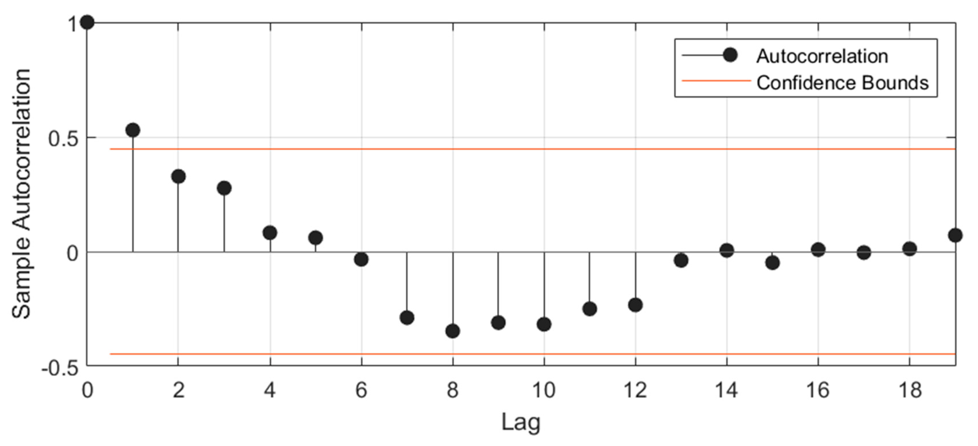
For ARIMA the model order (p, d, q) must be determined first. The KPSS test [35] was applied to the data of waste to determine whether the time series was stationary or not. If the test fails, the difference is taken, and the test is run again. d is the number of different operations required for the series to pass the test. p and q are calculated from the partial autocorrelation and autocorrelation functions (PACF and ACF). The value of q is the index of the last significant autocorrelation value in ACF. Considering Figure 2, q is 1 since it is lag of the last significant correlation. p is determined a similar way from the PACF. Once the model order is found, the model weights are optimized to minimize the MSE. Table 5 list ARIMA model order and optimized weights for each waste data. ARIMA (1,1,1) was found to be the optimum model for all waste data.
Table 6 compares the results of ETS and ARIMA models along with the coefficient of determination (R2). From the table we conclude that ARIMA provides better estimates compared to ETS except for domestic waste where ETS showed slightly better results. Both models gave poor results for dead animals’ waste. The negative R2 value for ETS indicates the model is not suitable for the data.

2.9. ML Modeling Methodologies

In this study, we adopted three modern ML methodologies including: RF, XGBOOST, and LSTM. In the following paragraphs we briefly introduce each method:
RF is a powerful ensemble learning method that operates by constructing multiple decision trees during training and outputting the average prediction (for regression) or majority vote (for classification) of the individual trees. Each tree is trained on a random subset of the data using a random selection of features, a technique known as bootstrap aggregating (bagging). This randomness helps reduce overfitting and improves generalization, making RF robust to noise and outliers. The method handles both numerical and categorical data efficiently, requires minimal hyperparameter tuning, and provides built-in feature importance evaluation. RF is particularly effective for medium-sized datasets with complex, nonlinear relationships, offering high accuracy while maintaining interpretability through feature contributions.
XGBoost is an advanced implementation of gradient-boosted decision trees designed for speed and performance. Unlike RF, which builds trees independently, XGBoost constructs trees sequentially, where each new tree corrects errors made by previous ones through gradient descent optimization. This iterative approach minimizes a user-defined loss function, enhancing predictive accuracy. XGBoost includes regularization terms to prevent overfitting and supports parallel processing, making it scalable for large datasets. Its flexibility allows customization of objective functions, evaluation metrics, and tree structures, while handling missing values automatically. XGBoost excels in structured/tabular data tasks, often outperforming other algorithms in competitions due to its precision, efficiency, and ability to capture intricate patterns in high-dimensional data.
LSTM networks are a specialized type of recurrent neural network (RNN) designed to model temporal dependencies and sequential data. Unlike traditional RNNs, LSTMs incorporate memory cells and gating mechanisms (input, forget, and output gates) to selectively retain or discard information over long sequences, effectively addressing the vanishing gradient problem. This architecture enables LSTMs to learn long-term patterns in time-series, text, or other sequential data, making them ideal for tasks like forecasting, natural language processing, and anomaly detection. While computationally intensive and requiring large datasets for training, LSTMs achieve state-of-the-art performance in complex sequential prediction problems by capturing nonlinear trends and dynamic temporal relationships that simpler models may miss. Their adaptability to variable-length inputs further enhances their utility in real-world applications. Together, RF, XGBoost, and LSTM represent versatile tools in ML, each excelling in specific domains RF for robust ensemble modeling, XGBoost for structured data optimization, and LSTM for sequential data mastery enabling accurate predictions across diverse problem types.

3. Results and Discussions

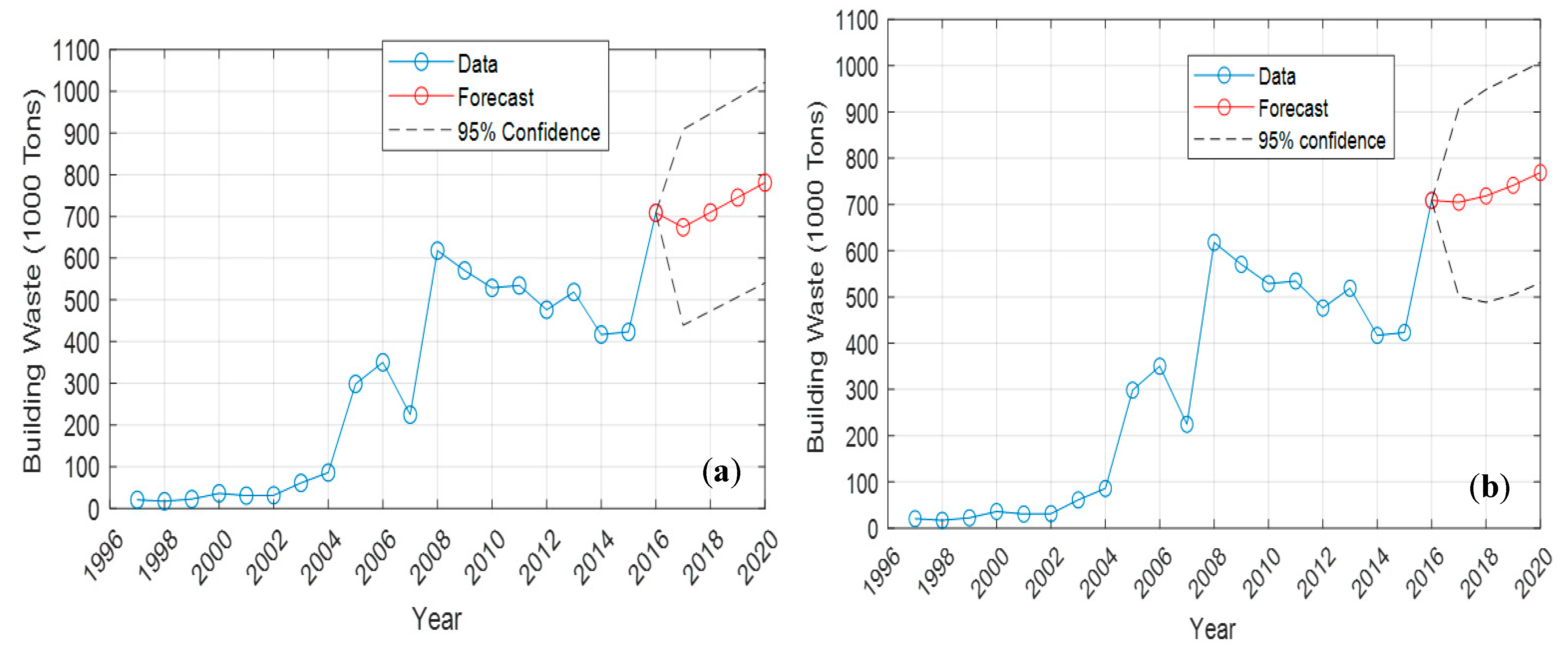
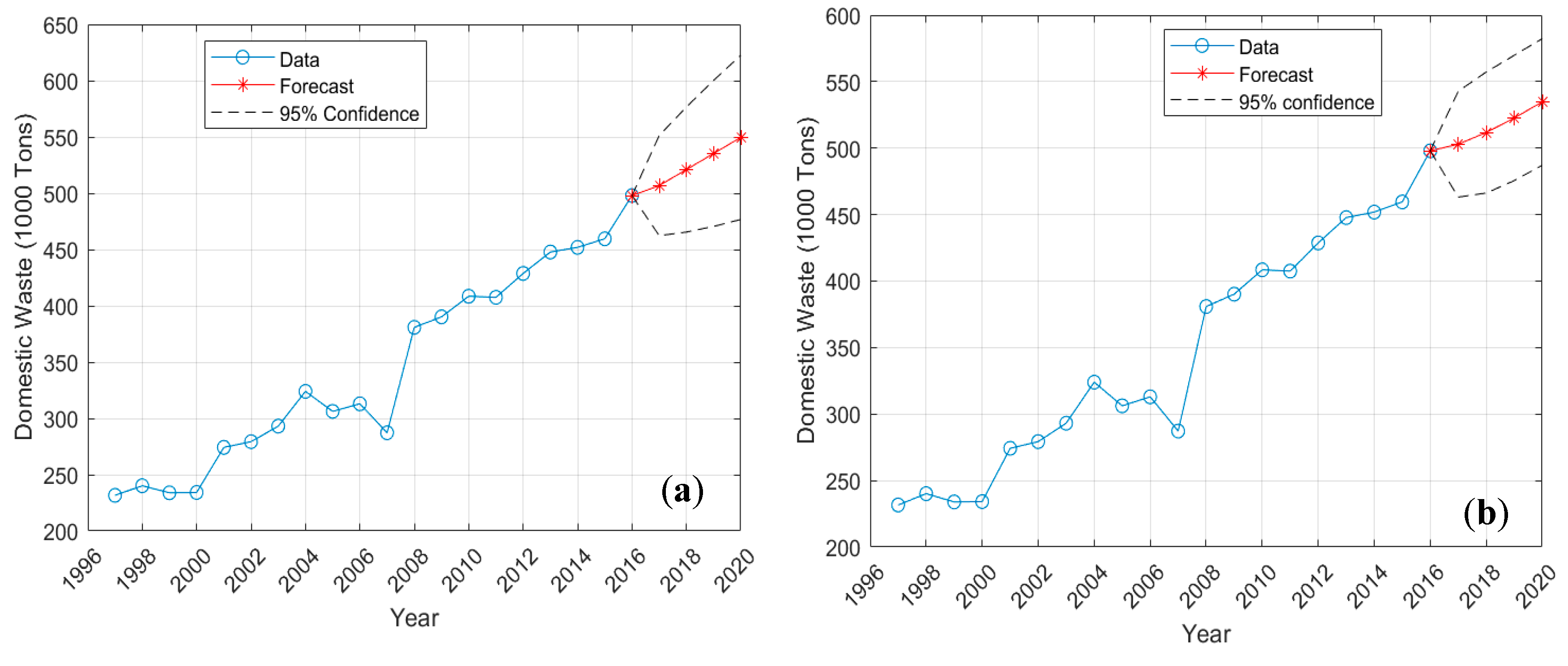
The forecasting results for the ETS and ARIMA models provided valuable insights into their performance across various waste streams, including building, commercial, domestic, dead animal, and liquid waste. ETS models excelled in identifying seasonal patterns and trends, offering reliable predictions for waste streams with stable periodic behavior. However, their accuracy was limited when faced with irregular or highly dynamic data. In contrast, ARIMA models proved effective for time series with strong linear trends and autocorrelations, delivering precise short-term forecasts. Despite their strengths, both models exhibited limitations in addressing the diverse and complex nature of waste generation patterns. These findings emphasize the need for advanced forecasting approaches that can better accommodate the variability inherent in different waste types. The obtained results are discussed in detail below, comparing model performance and exploring the potential benefits of integrating machine learning methods for enhanced accuracy. The forecasting results for the ETS and ARIMA models are presented in Figure 3, Figure 4, Figure 5, Figure 6 and Figure 7. Figure 3 shows the building waste forecast. Both models show approximately similar results, however ARIMA gives slightly tighter confidence intervals. The fluctuations in building waste led to a large confidence interval (±200 thousand tons) with a forecasted value of 750 thousand tons in 2020.
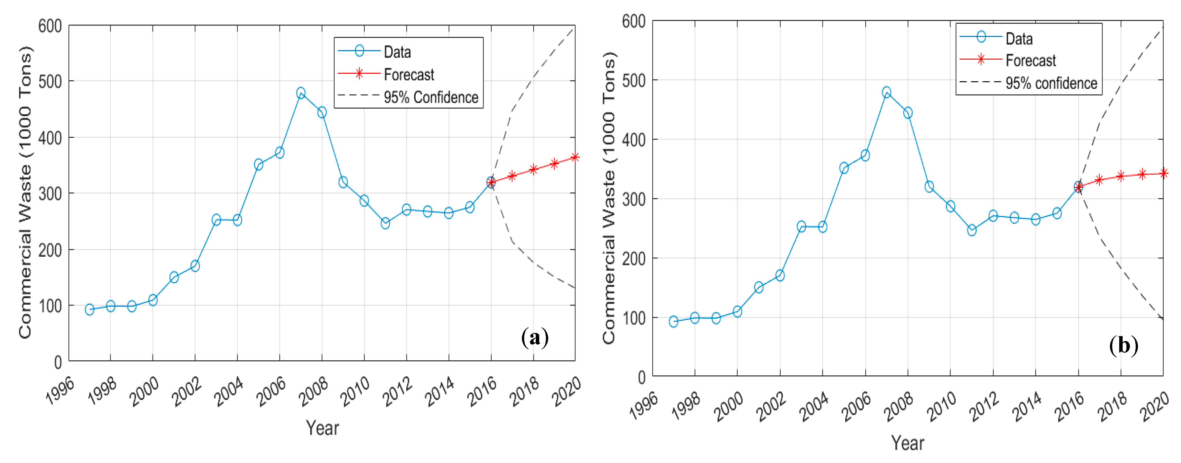
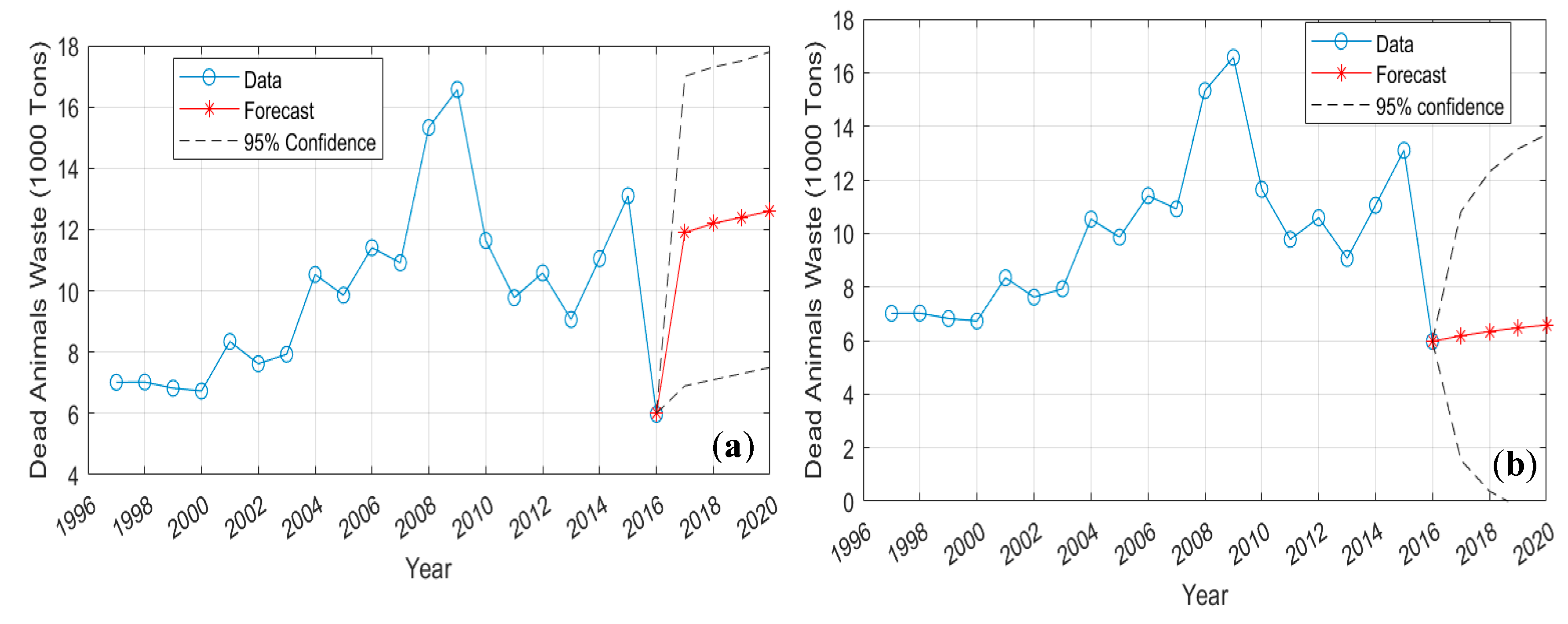
Figure 4 shows the forecast results for commercial waste. In this case, both models provided poor forecasts with large confidence intervals. Similarly with dead animals’ waste, Figure 5, poor forecasts are observed although ARIMA shows better performance compared to ETS.
The models show good performance with domestic waste. Domestic waste data have a clear trend with limited fluctuations and a small standard deviation compared to its mean as listed in Table 1. Hence, the models produced forecasts with tight confidence intervals (Figure 6).
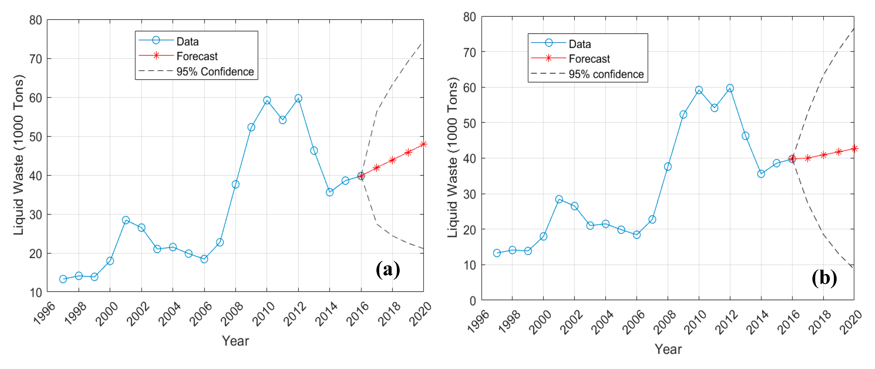
Figure 7 shows the forecast results for liquid waste. The data does not show a clear trend, and large fluctuations are observed. Moreover, the standard deviation is large, thus leading to poor forecasts.
All types of waste, except domestic waste, have large standard deviations, fluctuations within the time series, and changing trends (increasing then decreasing). This led to poor forecasts and indicates the existence of external factors that affect the amount of waste. These factors should be identified and included in the forecasting models to provide more accurate forecasts or employ machine learning algorithms. Currently only twenty observations are available for waste data. More data are required to improve the forecasting accuracy. ARIMA provided better performance compared to ETS except for domestic waste in terms of RMSE and MASE. MASE compares the performance of the model to the performance of the naïve forecasting method which simply takes the last value as a forecast for future observations. ETS model had a MASE greater than 1, Table 4 for all the data except domestic waste. An MASE of 1 or more means the naïve method provides more accurate forecasts than the model. ARIMA provided better forecasting performance, Table 5, than the naïve method except for dead animals’ and liquid wastes. Hence, ARIMA can be used to forecast building waste, and commercial waste. ETS provided more accurate forecasting for domestic waste. The naïve method will provide more accurate forecasts for liquid and dead animals’ wastes than ETS and ARIMA.
Three machine learning algorithms RF, XGBoost, and LSTM networks were employed for time series forecasting in this study. Each algorithm was selected to evaluate performance across different modeling approaches, from ensemble decision trees to deep learning. The comparative analysis aimed to determine the most effective method for predicting waste generation patterns, considering their varying complexities and temporal dependencies.
The dataset was divided into training (70%) and testing (30%) subsets using randomized splitting to prevent temporal bias. This partitioning strategy ensured that the models were trained on a representative sample while maintaining an independent test set for unbiased evaluation. Randomization during splitting helped avoid overfitting and ensured robust generalization across different time periods. The training set was used for model development and hyperparameter tuning, while the testing set provided a fair assessment of predictive accuracy.
Model performance was assessed using two key metrics: Mean Absolute Error (MAE) and Root Mean Squared Error (RMSE). MAE provided an interpretable measure of average prediction error in original units, while RMSE emphasized larger errors due to its squaring mechanism, making it sensitive to outliers. Both are commonly used metrics for evaluating regression models in machine learning. MAE measures the average absolute difference between predicted and actual values, providing a straightforward interpretation of error magnitude. It can be calculated using:
MAE = 1 n i = 1 n y i y ^ i
where y i is the actual value, y ^ i is the predicted value, and n is the number of observations. RMSE, on the other hand, emphasizes larger errors by squaring residuals before averaging, making it more sensitive to outliers. Its equation is:
RMSE = 1 n i = 1 n ( y i y ^ i ) 2
RMSE penalizes significant deviations more severely, making it useful when large errors are particularly undesirable. While MAE offers intuitive, scale-dependent error interpretation, RMSE provides a measure of error variability, with both metrics aiding in model comparison and performance assessment.
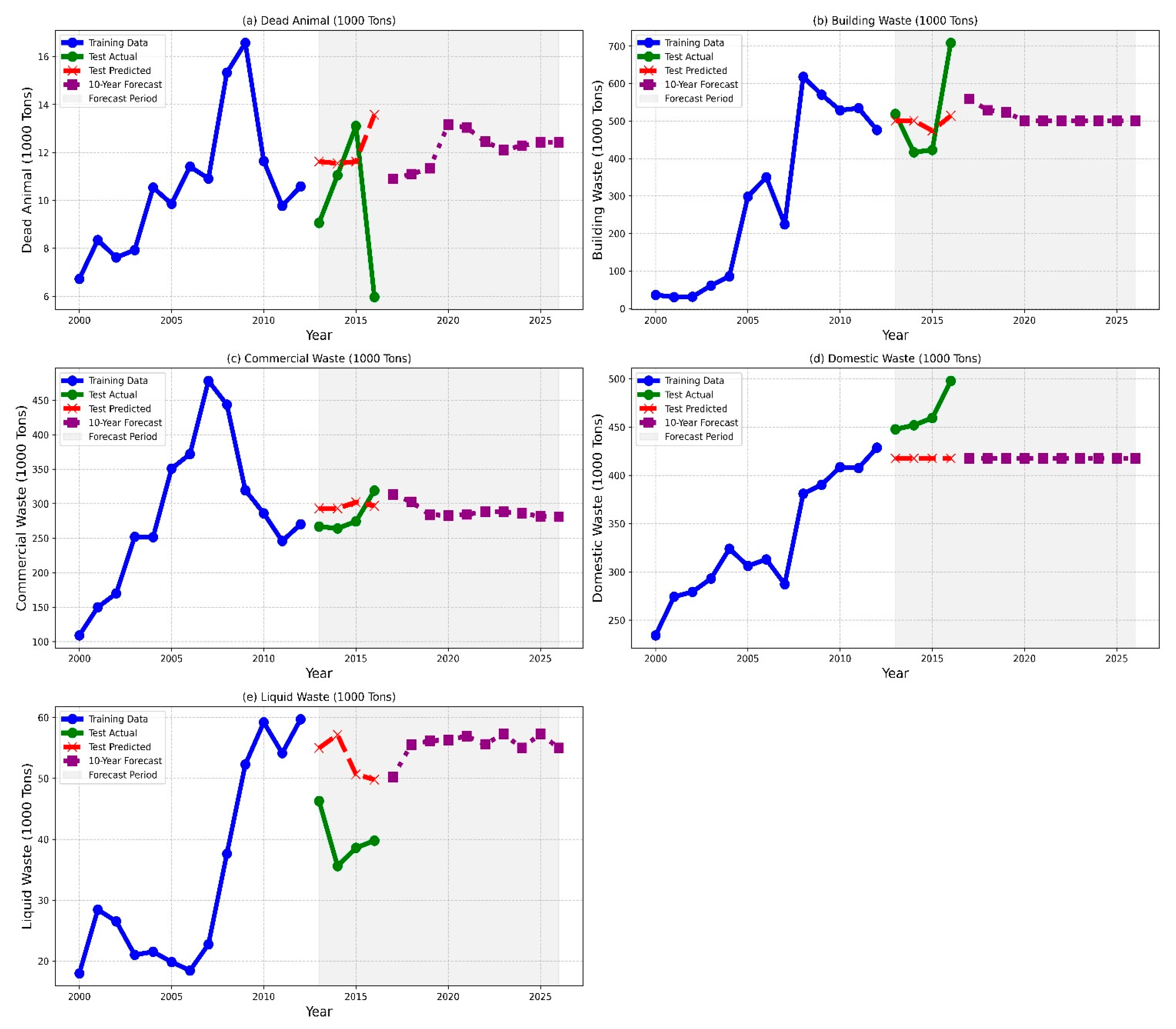
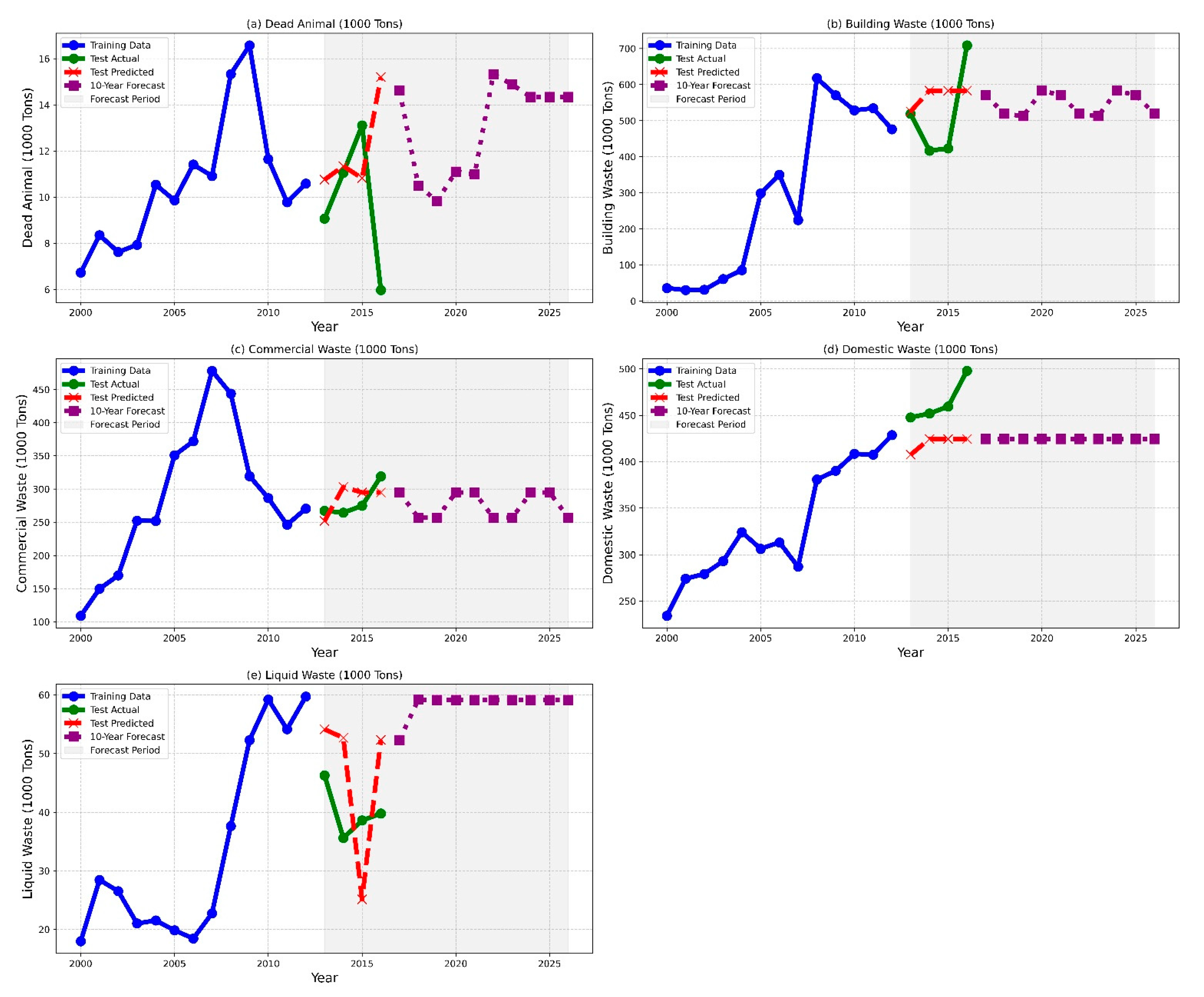
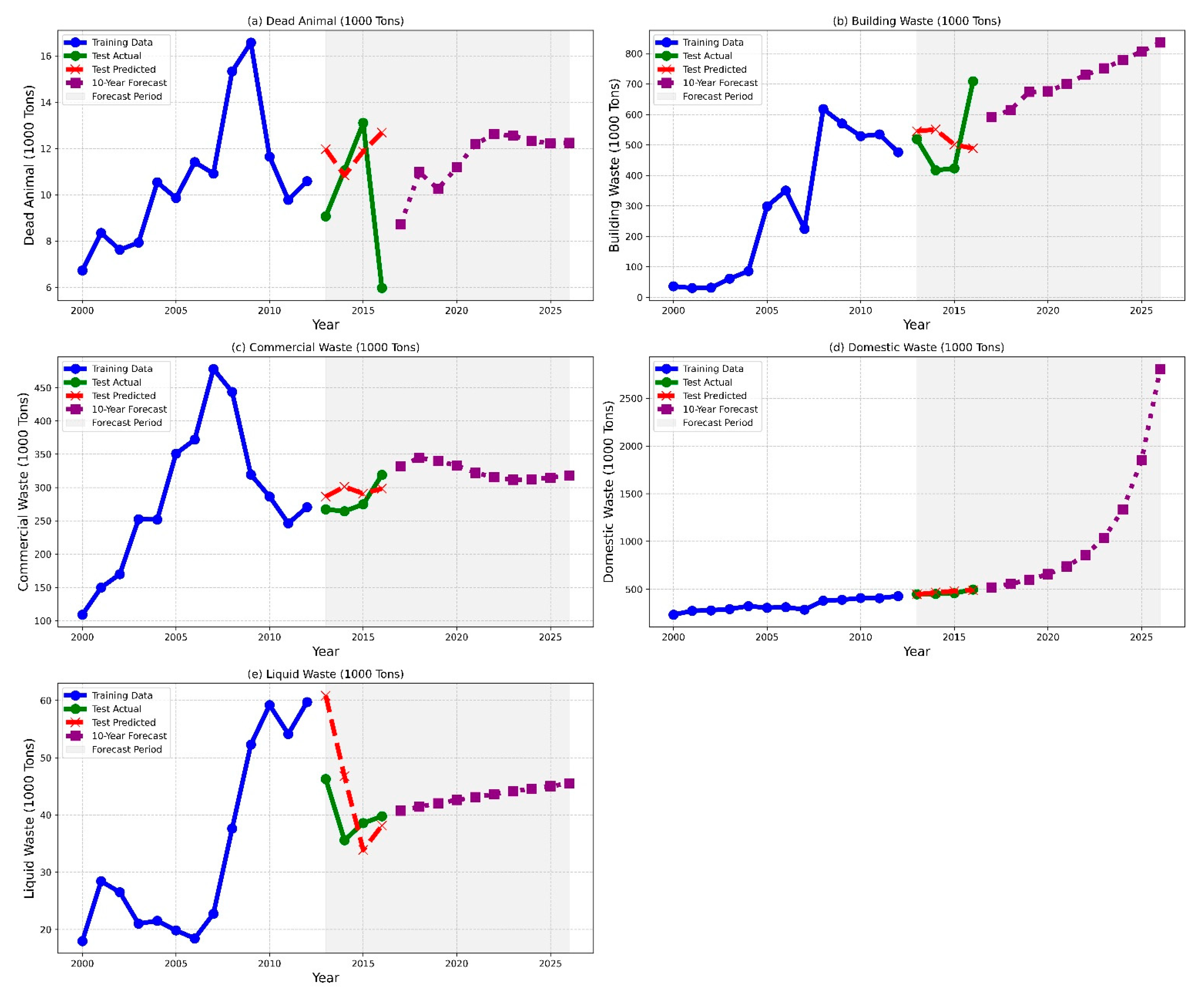
Among the three methods, LSTM demonstrated superior forecasting accuracy, as illustrated in Figure 8, Figure 9 and Figure 10. The performance hierarchy (LSTM > XGBoost > RF) was attributed to LSTM’s ability to capture long-term dependencies and nonlinear temporal patterns. Unlike tree-based methods, LSTMs autonomously learn features from sequential data, making them particularly effective for complex time series forecasting.
Table 7. Summary of ML models’ performance.
ML ModelMAE (Test)RMSE (Test)
DAWBWCWDWLWDAWBWCWDWLW
RF3.0387.0426.2046.8413.094.08109.3326.3450.8914.03
XGBOOST3.37114.6624.6144.0312.734.83131.4026.1147.4213.15
LSTM2.73110.7525.9211.538.233.53133.6727.8715.429.49

4. Conclusions

Accurate forecasting of waste volumes is an essential tool for strengthening waste management systems, optimizing resource allocation, and advancing environmental sustainability. This study has shown that forecasting cannot be approached with a one size fits all method; rather, different waste streams require different strategies. By combining ETS, ARIMA, RF, XGBoost, and LSTM, we developed an integrative framework that provides valuable insights into the comparative strengths and weaknesses of traditional statistical and machine learning approaches across five waste categories: building, commercial, domestic, dead animals, and liquid waste. The results demonstrated that ARIMA consistently outperformed ETS in forecasting building and commercial waste, particularly because of its ability to capture temporal dependencies and provide tighter confidence intervals. This accuracy is crucial in planning for construction debris processing and anticipating fluctuations driven by economic activities. Conversely, ETS produced more accurate forecasts for domestic waste, where the data exhibited consistent and stable patterns. This finding highlights the continued relevance of traditional models in structured and predictable waste streams. Forecasting irregular waste streams such as dead animals and liquid waste posed greater challenges. Their variability is often influenced by external and unpredictable drivers including disease outbreaks, seasonal changes, and industrial practices. In these cases, machine learning models demonstrated relative advantages. RF and XGBoost proved more effective at handling nonlinear interactions, while LSTM enhanced robustness by capturing long-term dependencies. Yet, naïve models sometimes performed comparably or better for these erratic categories, underscoring that model selection must be aligned with data characteristics rather than assumptions about complexity. The present study highlights that hybrid forecasting where statistical models are applied to consistent streams and machine learning to irregular ones offers a promising pathway forward. This methodological integration ensures that waste management systems can flexibly adapt to heterogeneous data and operational requirements. The operational significance of accurate forecasting is far reaching. For building and commercial waste, improved forecasts allow municipalities to plan capacity expansion, optimize construction debris recycling, and reduce dependence on landfills. For domestic waste, better predictions can guide collection schedules, enhance targeted recycling programs, and support operational efficiency in municipal services. Accurate forecasting of irregular streams such as dead animals and liquid waste is particularly valuable for emergency response and environmental monitoring, helping cities remain resilient to unexpected events such as disease outbreaks or industrial discharges. By improving forecasting accuracy, municipalities and policymakers can design more effective waste management strategies that align with Sustainable Development Goal 11 on sustainable cities and communities, Sustainable Development Goal 12 on responsible consumption and production, and Sustainable Development Goal 13 on climate action. This alignment underscores that forecasting is not only a technical matter but also a strategic enabler of global sustainability priorities. Despite these contributions, several limitations must be acknowledged. The most significant is data availability. Waste data are often limited, inconsistent, or aggregated at annual levels, which constrains the ability of models to capture short term fluctuations and seasonal trends. Expanding historical datasets with higher temporal granularity such as monthly or weekly observations would enhance forecasting precision. Another limitation is the restricted use of external explanatory variables. Waste generation is closely linked to socio economic, demographic, climatic, and regulatory conditions. Incorporating such variables would increase explanatory power, especially for irregular waste streams where variability cannot be explained by historical records alone. Machine learning models in particular could fully exploit multivariate inputs to uncover hidden dependencies if such data were available. A further limitation lies in model adaptability. The models used in this study were trained on static historical datasets. Sudden disruptions such as economic downturns, pandemics, or climate related events can rapidly invalidate past patterns. Developing adaptive and hybrid models that update dynamically as new data are generated represents a promising research direction to ensure resilience in forecasting performance.
The findings of this study open multiple avenues for future research. Expanding datasets both temporally and contextually should be a priority. Incorporating explanatory variables such as population growth, economic indicators, climate conditions, and regulatory shifts will help build more robust models. Methodological advances should focus on adaptive forecasting. Rolling origin cross validation, hybrid statistical and machine learning models, and online learning approaches could provide real time insights that remain relevant under shifting conditions. Stakeholder engagement must also be integrated into forecasting systems. Municipal authorities, private waste companies, and communities can validate assumptions, improve data collection, and ensure that forecasting outputs are practically applicable. Collaborative approaches will also help overcome one of the key barriers identified in this study, which is limited access to high quality standardized datasets. Forecasting should also be embedded within circular economy strategies. Accurate predictions enable targeted recycling, recovery, and reuse initiatives, thus reducing reliance on virgin resources and landfills. Machine learning algorithms can be applied not only for volume prediction but also for identifying material flows within waste streams and optimizing separation processes. These advances support SDG driven objectives by lowering greenhouse gas emissions, conserving resources, and promoting sustainable production and consumption. This study demonstrates that integrating ETS and ARIMA with RF, XGBoost, and LSTM provides a robust forecasting framework that leverages the complementary strengths of both statistical and machine learning approaches. By tailoring forecasting strategies to the specific characteristics of waste streams, municipalities and policymakers can anticipate fluctuations more accurately, improve operational efficiency, and design waste management systems that are resilient, adaptive, and environmentally sustainable. The broader implication is that forecasting is not simply about predicting numbers. It is about enabling smarter decision making for sustainable urban development. Accurate waste forecasting allows cities to plan infrastructure more effectively, allocate resources efficiently, and adopt circular economy practices that reduce environmental impact. Ultimately, this integrative data driven approach supports the creation of inclusive, safe, resilient, and sustainable cities, advances responsible consumption and production, and contributes to urgent climate action. Through these contributions, the study not only advances methodological understanding but also provides practical guidance for aligning waste management practices with global sustainability goals. Future work that builds upon these findings by expanding data, integrating external drivers, and developing adaptive models can further strengthen the role of forecasting as a cornerstone of environmental stewardship and urban resilience.

Author Contributions

N.A.: Conceptualization, methodology, resources, supervision, project administration, funding acquisition. A.L.: Conceptualization, methodology, validation, formal analysis, writing—original draft preparation. G.M.T.A.: Investigation, formal analysis, writing—review and editing. A.A. (Abdulaziz Alghamdi): Validation, resources, data curation. M.S.: Methodology, formal analysis, visualization. A.A. (Ahmed Alshahir): Data curation, investigation, writing—review and editing. S.A.: Validation, resources, supervision. I.A.: Writing—review and editing, visualization. F.M.A.: Investigation, project administration, supervision. All authors have read and agreed to the published version of the manuscript.

Funding

This work was funded by the Deanship of Graduate Studies and Scientific Research at Jouf University under grant No. (DGSSR-2025-NF-02-026).

Institutional Review Board Statement

Not applicable.

Informed Consent Statement

Not applicable.

Data Availability Statement

The data supporting the findings of this study are available from the corresponding author upon a raised request.

Acknowledgments

The authors gratefully acknowledge the financial support provided by the Deanship of Graduate Studies and Scientific Research at Jouf University under grant No. (DGSSR-2025-NF-02-026).

Conflicts of Interest

The authors declare no known conflicts of interest.

References

  1. Luo, B.; Su, Y.; Ding, X.; Chen, Y.; Liu, C. Modulation of initial CaO/Al2O3 and SiO2/Al2O3 ratios on the properties of slag/fly ash-based geopolymer stabilized clay: Synergistic effects and stabilization mechanism. Mater. Today Commun. 2025, 47, 113295. [Google Scholar] [CrossRef]
  2. Fu, H.; Tian, J.; Chin, C.-L.; Liu, H.; Yuan, J.; Tang, S.; Mai, R.; Wu, X. Axial compression behavior of GFRP-steel composite tube confined seawater sea-sand concrete intermediate long columns. Eng. Struct. 2025, 333, 120157. [Google Scholar] [CrossRef]
  3. Fu, H.; Zhao, H.; Pan, Z.; Wu, Z.; Chin, C.-L.; Ma, C.-K. Behaviour of corroded circular steel tube strengthened with external FRP tube grouting under eccentric loading: Numerical study. Structures 2023, 56, 104810. [Google Scholar] [CrossRef]
  4. Fu, H.; Tian, J.; Chen, S.; Chin, C.-L.; Ma, C.-K. Axial compressive performance of CFRP-steel composite tube confined seawater sea-sand concrete intermediate slender columns. Constr. Build. Mater. 2024, 441, 137399. [Google Scholar] [CrossRef]
  5. Adewuyi, A.Y.; Adebayo, K.B.; Adebayo, D.; Kalinzi, J.M.; Ugiagbe, U.O.; Ogunruku, O.O.; Samson, O.A.; Oladele, O.R.; Adeniyi, S.A. Application of big data analytics to forecast future waste trends and inform sustainable planning. World J. Adv. Res. Rev. 2024, 23, 2469–2479. [Google Scholar] [CrossRef]
  6. Singh, O. Forecasting trends in the generation and management of hazardous waste. In Hazardous Waste Management; Elsevier: Amsterdam, The Netherlands, 2022; pp. 465–489. [Google Scholar]
  7. Das, S.; Lee, S.-H.; Kumar, P.; Kim, K.-H.; Lee, S.S.; Bhattacharya, S.S. Solid waste management: Scope and the challenge of sustainability. J. Clean. Prod. 2019, 228, 658–678. [Google Scholar] [CrossRef]
  8. Tawo, O.E.; Mbamalu, M.I. Advancing waste valorization techniques for sustainable industrial operations and improved environmental safety. Int. J. Sci. Res. Arch. 2025, 14, 127–149. [Google Scholar] [CrossRef]
  9. Lebersorger, S.; Beigl, P. Municipal solid waste generation in municipalities: Quantifying impacts of household structure, commercial waste and domestic fuel. Waste Manag. 2011, 31, 1907–1915. [Google Scholar] [CrossRef]
  10. Lakhouit, A.; Shaban, M. Exploring sustainable solutions with machine learning algorithms: A focus on construction waste management. Clean Technol. Environ. Policy 2024, 27, 1297–1310. [Google Scholar] [CrossRef]
  11. Han, Z.; Liu, Y.; Zhong, M.; Shi, G.; Li, Q.; Zeng, D.; Zhang, Y.; Fei, Y.; Xie, Y. Influencing factors of domestic waste characteristics in rural areas of developing countries. Waste Manag. 2018, 72, 45–54. [Google Scholar] [CrossRef]
  12. Parihar, S.; Saini, K.P.S.; Lakhani, G.P.; Jain, A.; Roy, B.; Ghosh, S.; Aharwal, B. Livestock waste management: A review. J. Entomol. Zool. Stud. 2019, 7, 384–393. [Google Scholar]
  13. Lakhouit, A.; Shaban, M.; Alatawi, A.; Abbas, S.Y.; Asiri, E.; Al Juhni, T.; Elsawy, M. Machine-learning approaches in geo-environmental engineering: Exploring smart solid waste management. J. Environ. Manag. 2023, 330, 117174. [Google Scholar] [CrossRef] [PubMed]
  14. Xia, W.; Jiang, Y.; Chen, X.; Zhao, R. Application of machine learning algorithms in municipal solid waste management: A mini review. Waste Manag. Res. 2022, 40, 609–624. [Google Scholar] [CrossRef]
  15. Cruz, I.A.; Chuenchart, W.; Long, F.; Surendra, K.; Andrade, L.R.S.; Bilal, M.; Liu, H.; Figueiredo, R.T.; Khanal, S.K.; Ferreira, L.F.R. Application of machine learning in anaerobic digestion: Perspectives and challenges. Bioresour. Technol. 2022, 345, 126433. [Google Scholar] [CrossRef]
  16. Namoun, A.; Tufail, A.; Khan, M.Y.; Alrehaili, A.; Syed, T.A.; BenRhouma, O. Solid waste generation and disposal using machine learning approaches: A survey of solutions and challenges. Sustainability 2022, 14, 13578. [Google Scholar] [CrossRef]
  17. Wu, H.; Zuo, J.; Zillante, G.; Wang, J.; Yuan, H. Status quo and future directions of construction and demolition waste research: A critical review. J. Clean. Prod. 2019, 240, 118163. [Google Scholar] [CrossRef]
  18. Islam, R.; Nazifa, T.H.; Yuniarto, A.; Uddin, A.S.; Salmiati, S.; Shahid, S. An empirical study of construction and demolition waste generation and implication of recycling. Waste Manag. 2019, 95, 10–21. [Google Scholar] [CrossRef] [PubMed]
  19. Lupa, C.J.; Ricketts, L.J.; Sweetman, A.; Herbert, B.M. The use of commercial and industrial waste in energy recovery systems–A UK preliminary study. Waste Manag. 2011, 31, 1759–1764. [Google Scholar] [CrossRef]
  20. Khan, S.; Anjum, R.; Raza, S.T.; Bazai, N.A.; Ihtisham, M. Technologies for municipal solid waste management: Current status, challenges, and future perspectives. Chemosphere 2022, 288, 132403. [Google Scholar] [CrossRef]
  21. Dyson, B.; Chang, N.-B. Forecasting municipal solid waste generation in a fast-growing urban region with system dynamics modeling. Waste Manag. 2005, 25, 669–679. [Google Scholar] [CrossRef] [PubMed]
  22. Sobsey, M.D.; Khatib, L.A.; Hill, V.R.; Alocilja, E.; Pillai, S. Pathogens in animal wastes and the impacts of waste management practices on their survival, transport and fate. In Animal Agriculture and the Environment: National Center for Manure and Animal Waste Management White Papers; Rice, J.M., Caldwell, D.F., Humenik, F.J., Eds.; ASABE: St. Joseph, MI, USA, 2006; pp. 609–666. [Google Scholar]
  23. Lin, K.; Zhao, Y.; Kuo, J.-H.; Deng, H.; Cui, F.; Zhang, Z.; Zhang, M.; Zhao, C.; Gao, X.; Zhou, T.; et al. Toward smarter management and recovery of municipal solid waste: A critical review on deep learning approaches. J. Clean. Prod. 2022, 346, 130943. [Google Scholar] [CrossRef]
  24. Xia, J.; Liu, Y.; Yang, H.; Zhu, G. An Optimization Framework for Waste Treatment Center Site Selection Considering Nighttime Light Remote Sensing Data and Waste Production Fluctuations. Appl. Sci. 2024, 14, 10136. [Google Scholar] [CrossRef]
  25. Mushtaq, J.; Dar, A.Q.; Ahsan, N. Spatial–temporal variations and forecasting analysis of municipal solid waste in the mountainous city of north-western Himalayas. SN Appl. Sci. 2020, 2, 1161. [Google Scholar] [CrossRef]
  26. Hidalgo-Crespo, J.A.; Velastegui-Montoya, A.; Soto, M.; Rivas, J.L.A.; Zwolinski, P.; Riel, A.; Rivas-García, P. Improving urban waste management: A comprehensive study on household waste generation and spatial patterns in the Grand Guayaquil Metropolitan Area. Waste Manag. Res. J. Int. Solid Wastes Public Clean. Assoc. ISWA 2024, 42, 918–931. [Google Scholar]
  27. Eryganov, I.; Rosecký, M.; Šomplák, R.; Smejkalová, V. Forecasting the waste production hierarchical time series with correlation structure. Optim. Eng. 2025, 26, 781–803. [Google Scholar] [CrossRef]
  28. Smejkalová, V.; Šomplák, R.; Nevrlý, V.; Burcin, B.; Kučera, T. Trend forecasting for waste generation with structural break. J. Clean. Prod. 2020, 266, 121814. [Google Scholar] [CrossRef]
  29. Hyndman, R.; Athanasopoulos, G. Forecasting: Principles and Practice; OTexts: Melbourne, Australia, 2018. [Google Scholar]
  30. Holt, C.C. Forecasting seasonals and trends by exponentially weighted moving averages. Int. J. Forecast. 2004, 20, 5–10. [Google Scholar] [PubMed]
  31. Winters, P.R. Forecasting sales by exponentially weighted moving averages. Manag. Sci. 1960, 6, 324–342. [Google Scholar] [CrossRef]
  32. Gardner, E.S., Jr. Exponential smoothing: The state of the art. J. Forecast. 1985, 4, 1–28. [Google Scholar] [CrossRef]
  33. Box, G.E.; Jenkins, G.M.; Reinsel, G.C.; Ljung, G.M. Time Series Analysis: Forecasting and Control; John Wiley & Sons: Hoboken, NJ, USA, 2015. [Google Scholar]
  34. Hyndman, R.; Koehler, A.; Ord, K.; Snyder, R. Forecasting with Exponential Smoothing: The State Space Approach; Springer Science & Business Media: Berlin, Germany, 2008. [Google Scholar]
  35. Kwiatkowski, D.; Phillips, P.C.; Schmidt, P.; Shin, Y. Testing the null hypothesis of stationarity against the alternative of a unit root: How sure are we that economic time series have a unit root? J. Econom. 1992, 54, 159–178. [Google Scholar] [CrossRef]
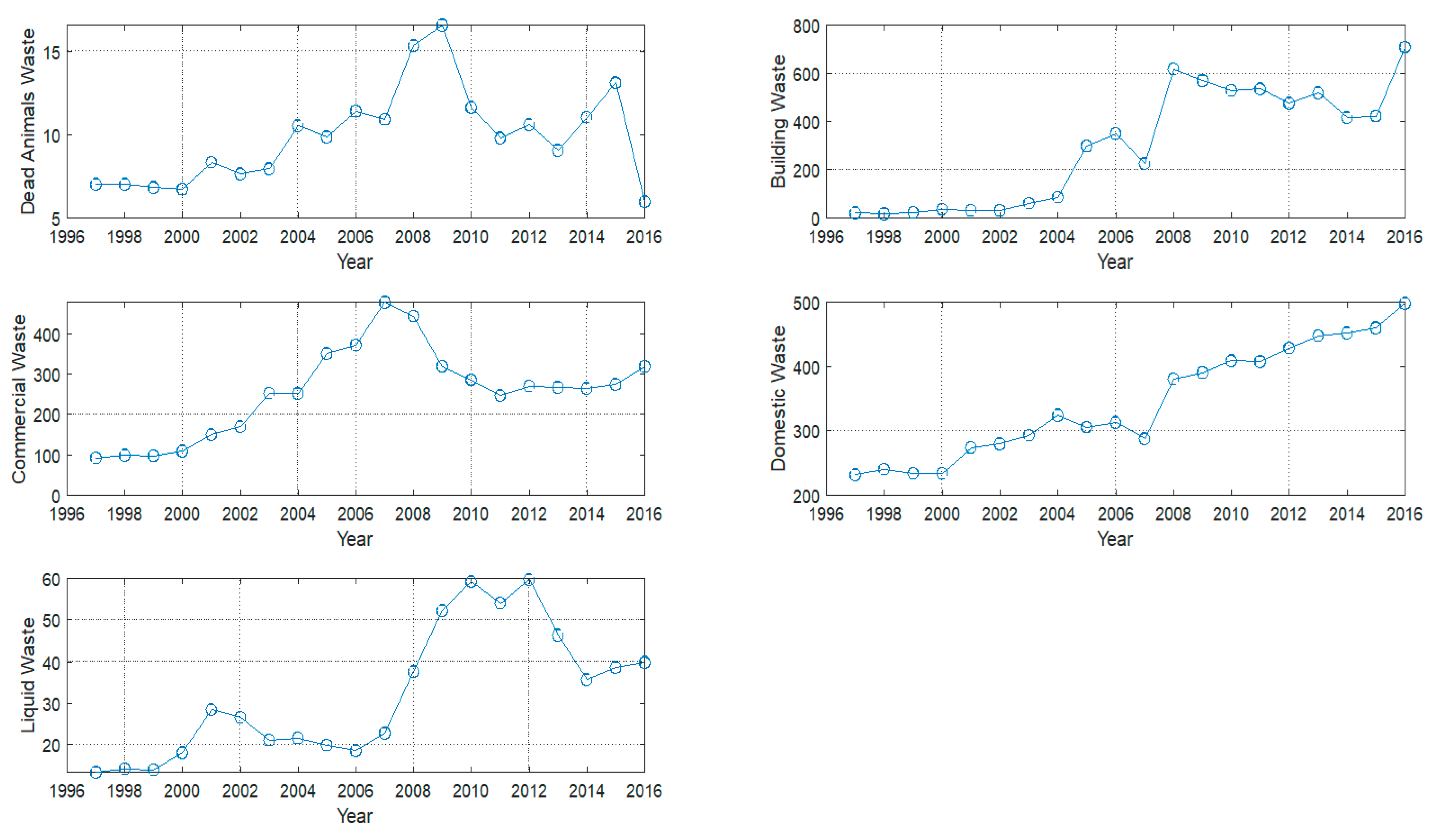
Figure 1. Waste Data (1000 Tons) 1997 to 2016.
Sustainability 17 08654 g001
Figure 2. Determination of q from the autocorrelation function.
Sustainability 17 08654 g002
Figure 3. Building waste: (a) ETS (b) ARIMA.
Sustainability 17 08654 g003
Figure 4. Commercial Waste: (a) ETS (b) ARIMA.
Sustainability 17 08654 g004
Figure 5. Dead Animals’ Waste: (a) ETS (b) ARIMA.
Sustainability 17 08654 g005
Figure 6. Domestic Waste: (a) ETS (b) ARIMA.
Sustainability 17 08654 g006
Figure 7. Liquid Waste: (a) ETS (b) ARIMA.
Sustainability 17 08654 g007
Figure 8. RF modeling results of forecasting five waste generation streams: (a) dead animal waste, (b) building waste, (c) commercial waste, (d) domestic waste, and (e) liquid waste.
Sustainability 17 08654 g008
Figure 9. XGBOOST modeling results of forecasting five waste generation streams: (a) dead animal waste, (b) building waste, (c) commercial waste, (d) domestic waste, and (e) liquid waste.
Sustainability 17 08654 g009
Figure 10. LSTM modeling results of forecasting five waste generation streams: (a) dead animal waste, (b) building waste, (c) commercial waste, (d) domestic waste, and (e) liquid waste. According to the summarized results in Table 7, there are noticeable reductions in MAE and RMSE compared to other methods which underscored LSTM’s advantage in handling dynamic waste generation trends. The study focused on the five waste streams: (a) dead animal waste (DAW), (b) building waste (BW), (c) commercial waste (CW), (d) domestic waste (DW), and (e) liquid waste (LW). LSTMs outperformed other models across most categories, particularly in capturing abrupt changes and long-term dependencies.
Sustainability 17 08654 g010
Table 1. Annual Waste Statistics (1000 Tons).
Stat./WasteDead AnimalBuildingCommercialDomesticLiquid
Minimum6.017.192.3231.613.3
Maximum16.6708.6478.2497.959.7
Mean9.9298.7255.7344.532.0
Standard Dev.2.87242.45110.9086.9215.64
Table 2. ETS models.
TrendSeasonality
None (N)Additive (A)Multiplicative (M)
None (N)(N, N)(N, A)(N, M)
Additive (A)(A, N)(A, A)(A, M)
Additive damped (Ad)(Ad, N)(Ad, A)(Ad, M)
Table 3. ETS models [29].
ADDITIVE ERROR MODELS
TrendSeasonal
NAM
N y t = l t 1 + ε t
l t = l t 1 + α ε t
y t = l t 1 + s t m + ε t
l t = l t 1 + α ε t
s t = s t m + γ ε t
y t = l t 1 s t m + ε t
l t = l t 1 + α ε t / s t m
s t = s t m + γ ε t / l t 1
A y t = l t 1 + b t 1 + ε t
l t = l t 1 + b t 1 + α ε t
b t = b t 1 + β ε t
y t = l t 1 + b t 1 + s t m + ε t
l t = l t 1 + b t 1 + α ε t
b t = b t 1 + β ε t
s t = s t m + γ ε t
y t = ( l t 1 + b t 1 ) s t m + ε t
l t = l t 1 + b t 1 + α ε t / s t m
b t = b t 1 + β ε t / s t m
s t = s t m + γ ε t / ( l t 1 + b t 1 )
Ad y t = l t 1 + ϕ b t 1 + ε t
l t = l t 1 + ϕ b t 1 + α ε t
b t = ϕ b t 1 + β ε t
y t = l t 1 + ϕ b t 1 + s t m + ε t
l t = l t 1 + ϕ b t 1 + α ε t
b t = ϕ b t 1 + β ε t
s t = s t m + γ ε t
y t = ( l t 1 + ϕ b t 1 ) s t m + ε t
l t = l t 1 + ϕ b t 1 + α ε t / s t m
b t = ϕ b t 1 + β ε t / s t m
s t = s t m + γ ε t / ( l t 1 + ϕ b t 1 )
MULTIPLICATIVE ERROR MODELS
TrendSeasonal
NAM
N y t = l t 1 ( 1 + ε t )
l t = l t 1 ( 1 + α ε t )
y t = ( l t 1 + s t m ) ( 1 + ε t )
l t = l t 1 + α ( l t 1 + s t m ) ε t
s t = s t m + γ ( l t 1 + s t m ) ε t
y t = l t 1 s t m ( 1 + ε t )
l t = l t 1 ( 1 + α ε t )
s t = s t m ( 1 + γ ε t )
A y t = ( l t 1 + b t 1 ) ( 1 + ε t )
l t = ( l t 1 + b t 1 ) ( 1 + α ε t )
b t = b t 1 + β ( l t 1 + b t 1 ) ε t
y t = ( l t 1 + b t 1 + s t m ) ( 1 + ε t )
l t = l t 1 + b t 1 + α ( l t 1 + b t 1 + s t m ) ε t
b t = b t 1 + β ( l t 1 + b t 1 + s t m ) ε t
s t = s t m + γ ( l t 1 + b t 1 + s t m ) ε t
y t = ( l t 1 + b t 1 ) s t m ( 1 + ε t )
l t = ( l t 1 + b t 1 ) ( 1 + α ε t )
b t = b t 1 + β ( l t 1 + b t 1 ) ε t
s t = s t m ( 1 + γ ε t )
Ad y t = ( l t 1 + ϕ b t 1 ) ( 1 + ε t )
l t = ( l t 1 + ϕ b t 1 ) ( 1 + α ε t )
b t = ϕ b t 1 + β ( l t 1 + ϕ b t 1 ) ε t
y t = ( l t 1 + ϕ b t 1 + s t m ) ( 1 + ε t )
l t = l t 1 + ϕ b t 1 + α ( l t 1 + ϕ b t 1 + s t m ) ε t
b t = ϕ b t 1 + β ( l t 1 + ϕ b t 1 + s t m ) ε t
s t = s t m + γ ( l t 1 + ϕ b t 1 + s t m ) ε t
y t = ( l t 1 + ϕ b t 1 ) s t m ( 1 + ε t )
l t = ( l t 1 + ϕ b t 1 ) ( 1 + α ε t )
b t = ϕ b t 1 + β ( l t 1 + ϕ b t 1 ) ε t
s t = s t m ( 1 + γ ε t )
Table 4. ETS model parameters and statistics.
ETS Model
αβγRMSEMASE
Building Waste0.1260.00101221.33
Commercial Waste0.9980.001054.01.05
Dead Animals Waste0.1000.00103.372.20
Domestic Waste0.7500.001011.50.45
Liquid Waste0.9000.00109.471.81
Table 5. ARIMA model parameters and statistics.
WasteOrder
(p, d, q)
ϕθcRMSEMASE
Building(1,1,1)0.521−115.73104.070.98
Commercial(1,1,1)0.514−0.265048.430.88
Dead Animals(1,1,1)0.807−102.371.44
Domestic(1,1,1)0.554−16.0420.310.65
Liquid(1,1,1)−0.0600.51806.531.14
Table 6. Comparison between ETS and ARIMA models.
WasteETSARIMA
MASERMSER2MASERMSER2
Building1.331220.7480.98104.070.816
Commercial1.0554.00.7630.8848.430.809
Dead Animals2.203.37−0.3771.442.370.318
Domestic0.4511.50.9820.6520.310.945
Liquid1.819.470.6331.146.530.826
Disclaimer/Publisher’s Note: The statements, opinions and data contained in all publications are solely those of the individual author(s) and contributor(s) and not of MDPI and/or the editor(s). MDPI and/or the editor(s) disclaim responsibility for any injury to people or property resulting from any ideas, methods, instructions or products referred to in the content.