Coupling a Physically Based Hydrological Model with a Modified Transformer for Long-Sequence Runoff and Peak-Flow Prediction

Abstract

Climate change and human activities are intensifying the hydrologic cycle and increasing extreme events, challenging accurate prediction. This study builds on the Transformer architecture by introducing a sliding time window and runoff classification mechanism, enabling high-precision long-term runoff forecasting and significantly improving the simulation of extreme floods. However, the generalization ability of data-driven models remains limited in non-stationary environments. To address this issue, we further propose a hybrid framework that couples the process-based GBHM with the enhanced Transformer via bias correction. This fusion leverages the strengths of both models: the process-based model explicitly captures topographic heterogeneity, the spatial distribution of meteorological forcings, and their temporal variability, while the data-driven model excels at uncovering latent relationships among hydrological variables. The results demonstrate that the coupled model significantly outperforms traditional approaches in peak-flow prediction and exhibits superior robustness and generalizability under changing environmental conditions.

1. Introduction

The Intergovernmental Panel on Climate Change (IPCC) Sixth Assessment Report underscores that human-induced climate change is increasing the frequency of extreme precipitation and flood events [1,2]. Globally, every additional 1 °C of warming intensifies extreme daily precipitation by about 7%, thereby increasing the likelihood of both extreme floods and severe droughts [3]. The abruptness and destructive power of such events pose significant risks to natural ecosystems and human societies [4,5]. Over the past four decades, the average economic losses attributable to climate change and hydrological extremes have increased roughly tenfold [6].

Hydrological models are principal tools that leverage meteorological, topographic, and soil data to simulate hydrological processes, enabling event forecasting, risk assessment, driver attribution, and management evaluation [7,8]. Under the combined effects of climate change and human activities, physically based distributed hydrological models—owing to their mechanistic foundations—often perform well in hydrological simulation [9,10]. Nevertheless, structural, data quality, and parameterization constraints still limit accuracy in reproducing extreme hydrological events, especially catastrophic floods, thus calling for targeted refinement [11,12].

Data-driven hydrological models have gained substantial traction for extreme event simulation as hydro-meteorological data availability has grown, information technology has advanced, and computational power has increased. Machine learning paradigms evolved from shallow learners (e.g., SVM, DT, RF) to multilayer deep neural networks [13,14,15,16,17]. CNNs, RNNs/LSTMs, and GANs are widely used across disciplines and in hydrology, supporting short-lead-time flood forecasting, medium- to long-term runoff simulation, and projections of hydrological variables with competitive accuracy in diverse basins [18,19,20,21,22,23,24]. The Transformer, introduced by Vaswani et al. in 2017 [25], was initially developed for natural language processing [26] and later extended to computer vision, speech recognition, knowledge graphs, and long-sequence forecasting [27,28]. Since 2021, the architecture has been progressively adopted for hydrological applications [29,30].

However, empirical evidence indicates that standard Transformer architectures are suboptimal for rainfall–runoff tasks and benefit from hydrology-aware revisions [31,32,33]. Three principal approaches have emerged: (i) structural simplification—e.g., RRS-Former removing the encoder–decoder interface and cross-attention and encoder-only variants for SPI-6, evaporation, and flood-peak prediction [33,34,35,36]; (ii) architectural adjustment—e.g., residual 1-D convolutions and BatchNorm for small-batch stability on CAMELS and dual-encoder schemes with year–month embeddings [29,32]; (iii) hybridization with auxiliary networks—e.g., multiresolution convolutional trees with pyramid attention masks that reconcile short-term features with long-range dependencies [37]. Hybrid configurations further elevate performance, including CNN–Transformer pairings to map global SST/MSLP to local monthly runoff [38], LSTM–Transformer encoders [39], and adaptive random-search hyperparameter tuning [31], each outperforming standard LSTM/MLP/Transformer baselines.

Data-driven models, including Transformer, can extract latent connections among hydrological variables and, with appropriate training, accurately describe complex hydrologic cycles [40]. Their performance, however, is highly contingent on data quantity, preprocessing, and input selection [41]. Lacking physical constraints, such models are prone to overfitting, undermining credibility and limiting long-range runoff projections under changing environmental conditions [42]. Physically based watershed models, by contrast, explicitly represent terrain heterogeneity and the spatial variability in meteorological drivers [43], affording clear advantages under changing environmental conditions. Consequently, recent work has coupled process-based and data-driven approaches to harness their complementary strengths, providing a promising pathway for hydrological simulation in evolving climates [19,44,45].

Existing studies categorize hybrid hydrological models that fuse physically based and data-driven approaches into three groups [46]: (i) models that replace intermediate physical processes with data-driven surrogates [47,48,49,50]; (ii) models that substitute computationally intensive sub-basins within physical simulators [46]; and (iii) models that learn and correct systematic forecast errors of physical models [51,52]. Beyond these schemes, some studies extract intermediate outputs—e.g., soil moisture [53,54], baseflow [55], infiltration [56], and snow depth [57]—to inform data-driven training; however, such approaches remain fundamentally data-centric. Among the three hybrid strategies, error-learning models, where data-driven components explicitly capture the systematic forecast bias of process-based simulators, are the most prevalent [46]. Physically based models, limited by input data precision and theoretical assumptions, often yield autocorrelated biases; modeling these deviations and expressing observed discharge as the sum of the physical output and the learned error term markedly improves predictive accuracy [58]. Early ANN-based correction of conceptual and process-based models (e.g., SMAR, TOPMODEL, GR4J, IHAC, ARMA, kinematic-wave models), followed by MLP/LSTM couplings, consistently outperformed standalone physical or data-driven baselines across multiple basins and countries [44,45,59,60,61,62,63].

Despite increasing adoption of Transformer-based runoff models, reported gains remain concentrated at single-step or short- to medium-term horizons, with insufficient accuracy for decadal-scale runoff and high-flow events and with limited robustness and physical interpretability under changing environmental conditions [64].

This study aims to improve long-sequence runoff prediction and extreme flood simulation under changing environmental conditions and to close a gap whereby Transformer-based runoff models report gains mainly at single-step or short- to medium-term horizons, with inadequate accuracy for decadal-scale runoff and high-flow floods. We (i) design a fully masked Transformer with a sliding time window, (ii) introduce a runoff-classification scheme to up-weight rare extremes, and (iii) couple the enhanced network with the process-based GBHM via residual bias correction. We demonstrate that the coupled model reduces peak-flow underestimation and improves robustness across climate/land surface shifts. This work delivers an enhanced Transformer architecture, a classification-based training pipeline for extremes, and a GBHM–RRT (RCGR) framework benchmarked on multi-decadal records. The remainder of this article presents the study area and data (Section 2), methods (Section 3), results (Section 4), and discussion and conclusions (Section 5).

2. Study Area and Data

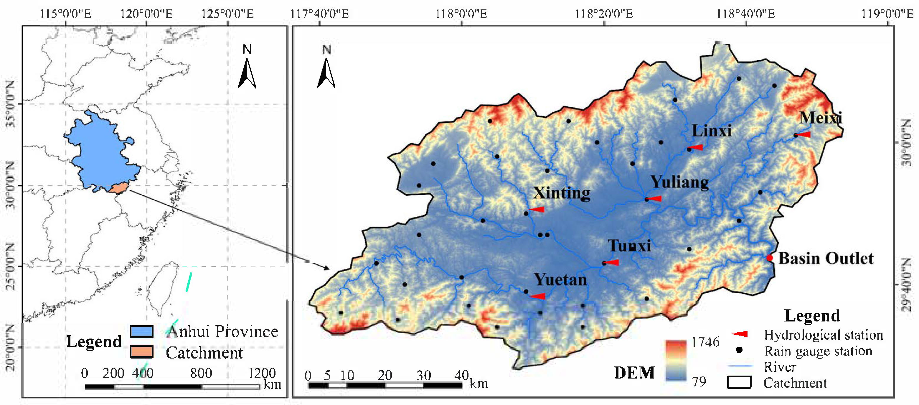
This study primarily focuses on the upper part of the Xin’an River Basin (XRB) (117°38′~118°53′ E, 29°27′~30°14′ N), covering an area of 5615 km² (Figure 1). The XRB belongs to a middle and low mountain hill region, characterized by high altitudes in the center and low altitudes around it, with a large relative elevation difference [65]. Elevations range from 99 to 1715 m, and landforms are predominantly hilly. The spatial and temporal distribution of water in the basin is uneven. The average annual runoff over the years is 6.53 billion m³, with the maximum annual runoff recorded in 1999 at 11.9 billion m³ and the minimum annual runoff recorded in 1978 at 3.2 billion m³. Precipitation in the basin alternates between wet and dry years, with 2019 experiencing a once-in-50-years drought, followed by a once-in-50-years flood in the following year. Runoff from April to July accounts for approximately 50–60% of the total annual runoff, with early onset and a sharp decline in late summer. The maximum monthly runoff accounts for about 20% of the annual runoff, while the minimum monthly runoff is less than 2% of the annual runoff [66].

Topographic data for the XRB is sourced from the ASTER GDEM V3 data product (https://doi.org/10.5067/ASTER/ASTGTM.003 [accessed on 22 September 2025]), with a resolution of 30 m [67]. Soil data is sourced from the “Chinese Soil Dataset (v1.1)” based on the World Soil Database (HWSD) from the National Tibetan Plateau Data Center (http://data.tpdc.ac.cn/), with a spatial resolution of 1000 m [68,69]. Land use data were sourced from the China Multi-period Land Use/Land Cover Change dataset (CNLUCC) at 30 m resolution for the years 1980, 1990, 2000, 2010, and 2018 (http://www.resdc.cn/).

For hydrological observations, the basin hosts 40 rain-gauge stations and 6 hydrological (streamflow) stations. All precipitation and discharge records from these stations for 1970–2019 were obtained from the Hydrological Yearbook of the People’s Republic of China-Qiantang River Basin, compiled by the Hydrology Bureau, Ministry of Water Resources, Beijing, China. Additionally, there are 5 national meteorological stations in the XRB, mainly located in the northern region of the basin. Therefore, meteorological stations within a 100 km radius from the basin’s boundary are also considered as supplementary data sources, resulting in a total of 37 stations, including 3 benchmark stations, 9 basic stations, and 25 general stations. These meteorological records for 1970–2019, including precipitation, atmospheric pressure, relative humidity, sunshine duration, air temperature, and wind speed, were obtained from the National Meteorological Science Data Center (http://data.cma.cn/). Due to the shorter data recording periods for some hydrological stations, this study primarily uses daily flow data from the Tunxi, Yuetan, and Yuliang stations, which have better data quality and longer time series, with other stations serving as reference points.

3. Methodology

Under the dual influences of climate change and intensified human activities, physically based distributed hydrological models have demonstrated strong capabilities in simulating hydrological processes due to their mechanistic foundation [70,71]. However, their performance in simulating extreme hydrological events—particularly severe flood events—remains limited by structural complexities, data quality constraints, and parameter uncertainties [72,73]. With the increasing availability of hydrometeorological data, advancements in information technologies, and enhanced computational power, data-driven hydrological models have garnered growing attention, offering promising avenues for improving the simulation of extreme events [74]. To address these challenges and elevate overall modeling performance, this study integrates an enhanced Transformer-based data-driven architecture with the GBHM distributed hydrological framework, aiming to achieve more robust and accurate simulations under non-stationary and extreme conditions.

3.1. Transformer Model

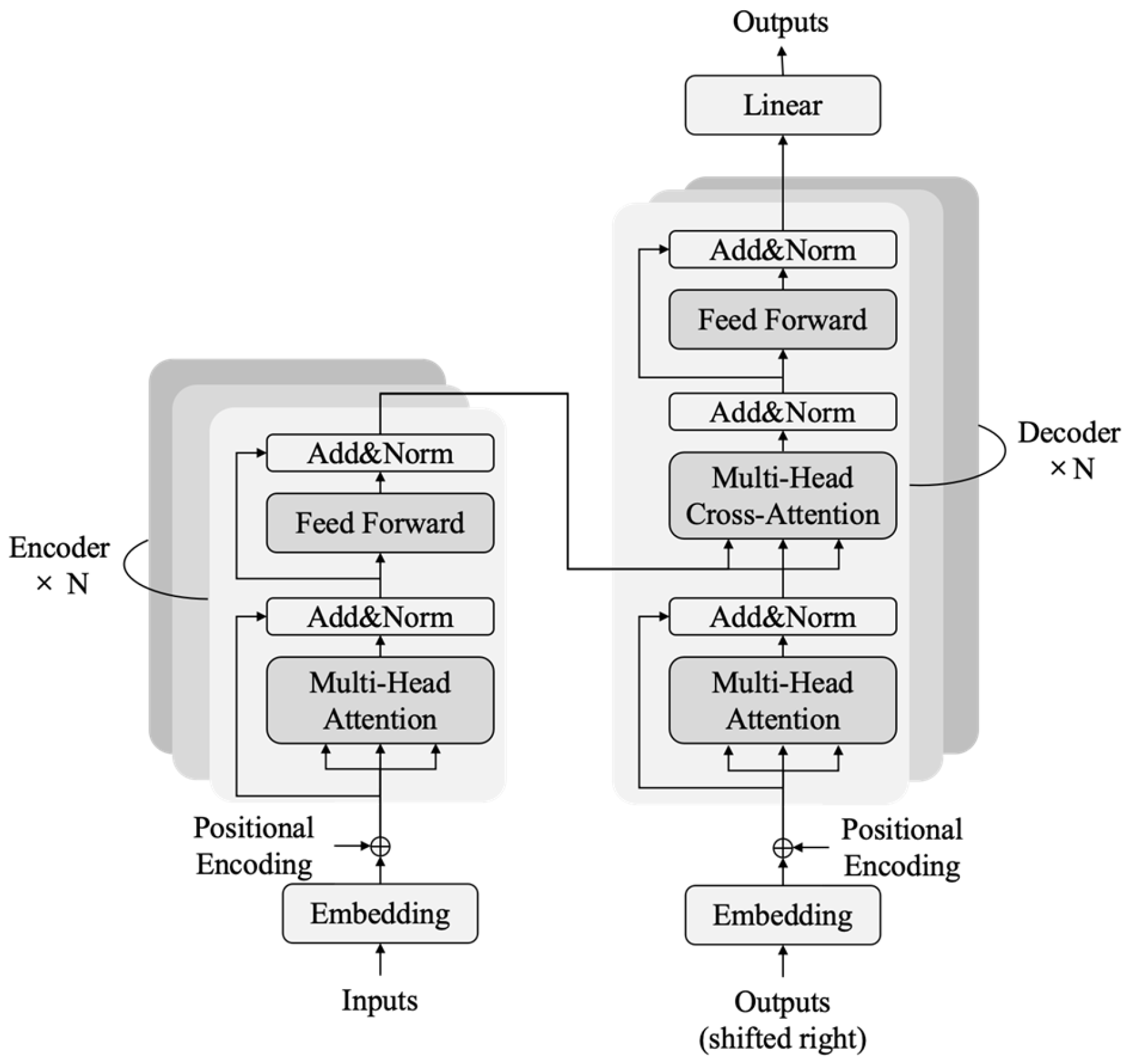
The Transformer is a neural network architecture based on the attention mechanism, proposed by Vaswani et al. in 2017 [25]. Unlike traditional sequence processing methods, it relies entirely on the attention module to compute the representations of the input and output [75]. Through the self-attention mechanism, the Transformer can directly model the dependencies between any two positions in a time series, without relying on a fixed sequence order [28]. This architecture can flexibly capture global features while adjusting the strength of connections between different positions, thereby demonstrating outstanding performance in handling complex temporal tasks. The structure of the Transformer model is shown in Figure 2:

3.2. Modified Transformer Model

Original Transformer models compute multi-head attention globally over the entire input sequence. When the sequence is long, this not only leads to high computational costs but may also overlook local short-term dependency features [76], which is unfavorable for simulating extreme hydrological events. To address these issues, the improved model introduces a time window mechanism. By limiting the attention computation scope, it achieves more efficient and temporally adaptive local attention calculations. Simultaneously, it employs a sliding window mechanism to balance the relationship between local features and global features across multiple time windows.

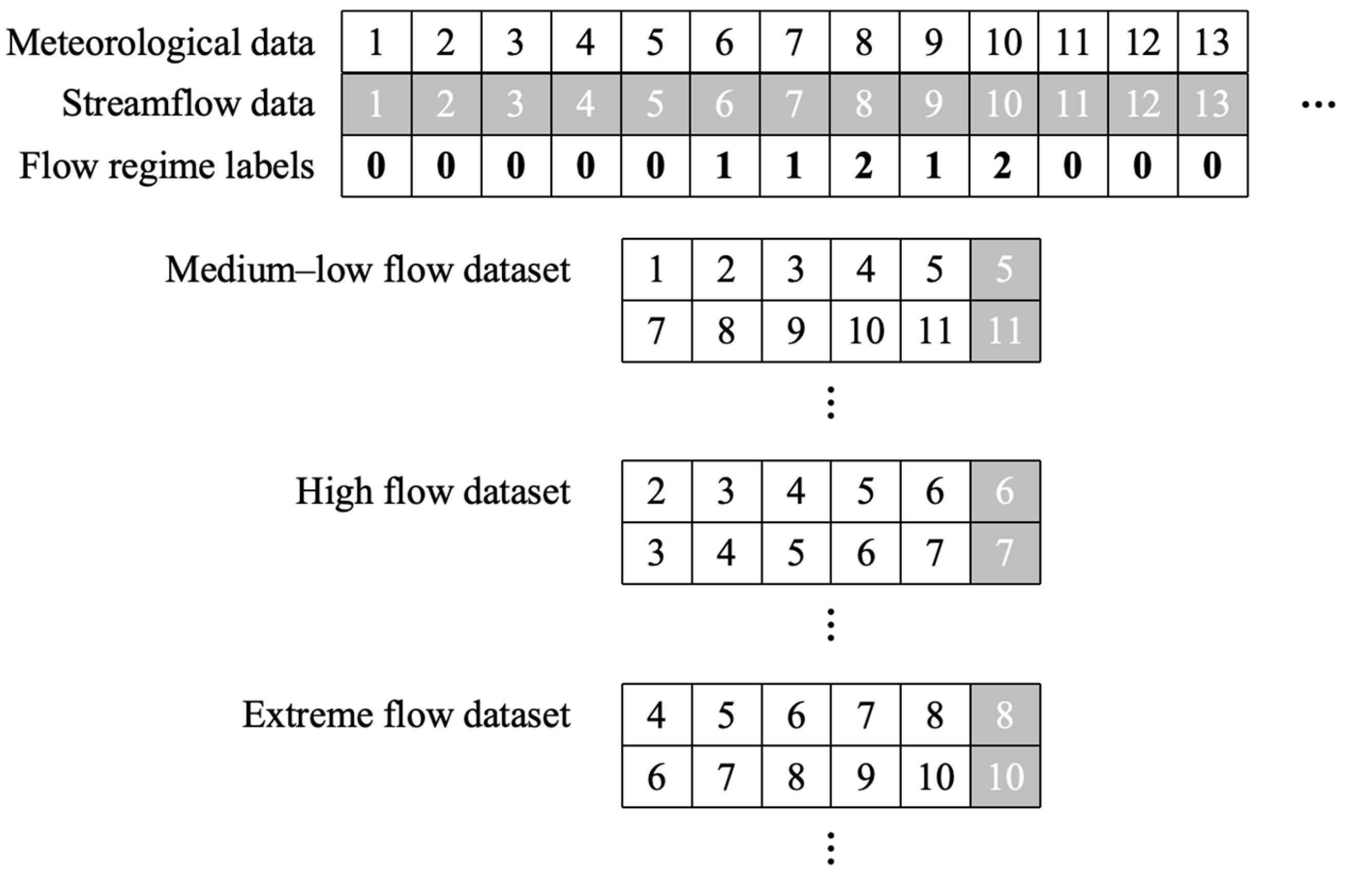
Although the introduction of the time window mechanism can enhance the model’s ability to capture local information, extreme events occur infrequently in the entire training dataset. This leads to their insufficient representation during the model training process, making it often difficult for the model to accurately capture and predict these rare events. In actual predictions, this is manifested as the model typically underestimating extreme flow events [77]. To address the issue of insufficient representation of extreme events due to their low occurrence frequency in the training dataset, classification simulation techniques are further introduced [78,79]. The principle of classification simulation is to classify the meteorological sequences corresponding to medium-low flow, high flow, and extremely high flow based on the relationship between meteorological and runoff sequences, forming three datasets. These three datasets are then separately trained and predicted.

(1)

Local Attention Scope

In the original Transformer, the calculation ranges of Q, K, and V cover the entire input sequence, resulting in a matrix dimension of $n\times n$. In the improved model, the time window mechanism restricts the calculation ranges of Q, K, and V to focus only on data within the time window. Therefore, the matrix dimension is limited to $w\times w$, where $w$ is the size of the time window. This effectively captures short-term dependencies within the window.

(2)

Sliding Window Mechanism

By calculating attention for each window individually, the model captures local features. Introducing a sliding window mechanism enables the model to learn and acquire global features. The time series $X=\left[x_1,x_2,\dots ,x_n\right]$ is divided into multiple time windows, each containing w time steps. For the k-th window $X_k$, it is represented as:

$$X_k=\left[x_{\left(k - 1\right)s + 1},x_{\left(k - 1\right)s + 2},\dots ,x_{\left(k - 1\right)s + w}\right],$$

(1)

where $s$ is the sliding step size. To prevent the time window from splitting a complete flood process and causing omissions in information learning, the sliding step size $s$ is set to 1. That is, each time the window slides, only the first element is removed from the window, all subsequent elements are retained, and a new element is introduced.

(3)

Transformer for classification

Under the improvement of local attention range and sliding window mechanisms, the Transformer model was modified for classification tasks. First, the loss function was changed to the Cross-Entropy Loss, which is widely used in classification problems and measures the difference between the predicted probability distribution and the true distribution. One-hot encoding was used for handling labels. This encoding method converts discrete category labels into a format suitable for neural network processing, i.e., each category label is converted into a vector where all elements are 0 except for one position, which is 1 and corresponds to the category. For example, medium-low flow is represented as [1, 0, 0], high flow as [0, 1, 0], and extremely high flow as [0, 0, 1]. A Softmax activation function was added to the model’s output to convert the raw outputs into probabilities for each category.

The Transformer for classification also uses the sliding window method. As shown in Figure 3, taking a 5-day sliding window as an example, each time step corresponds to a classification label of 0, 1, or 2, representing medium-low flow, high flow, and extremely high flow, respectively. The flow classification label for day n determines the time window from day n − 4 to day n and assigns it to the corresponding classification flow dataset. For example, if the flow classification label for day 8 is 2, indicating extremely high flow, the meteorological data from days 4 to 8 form a time window and are added to the extremely high flow dataset. The observed flow for day 8 also enters and serves as the basis for evaluating the model’s simulation performance. However, the observed flow value itself is not input into the model as a known variable.

3.3. Physically Based Model

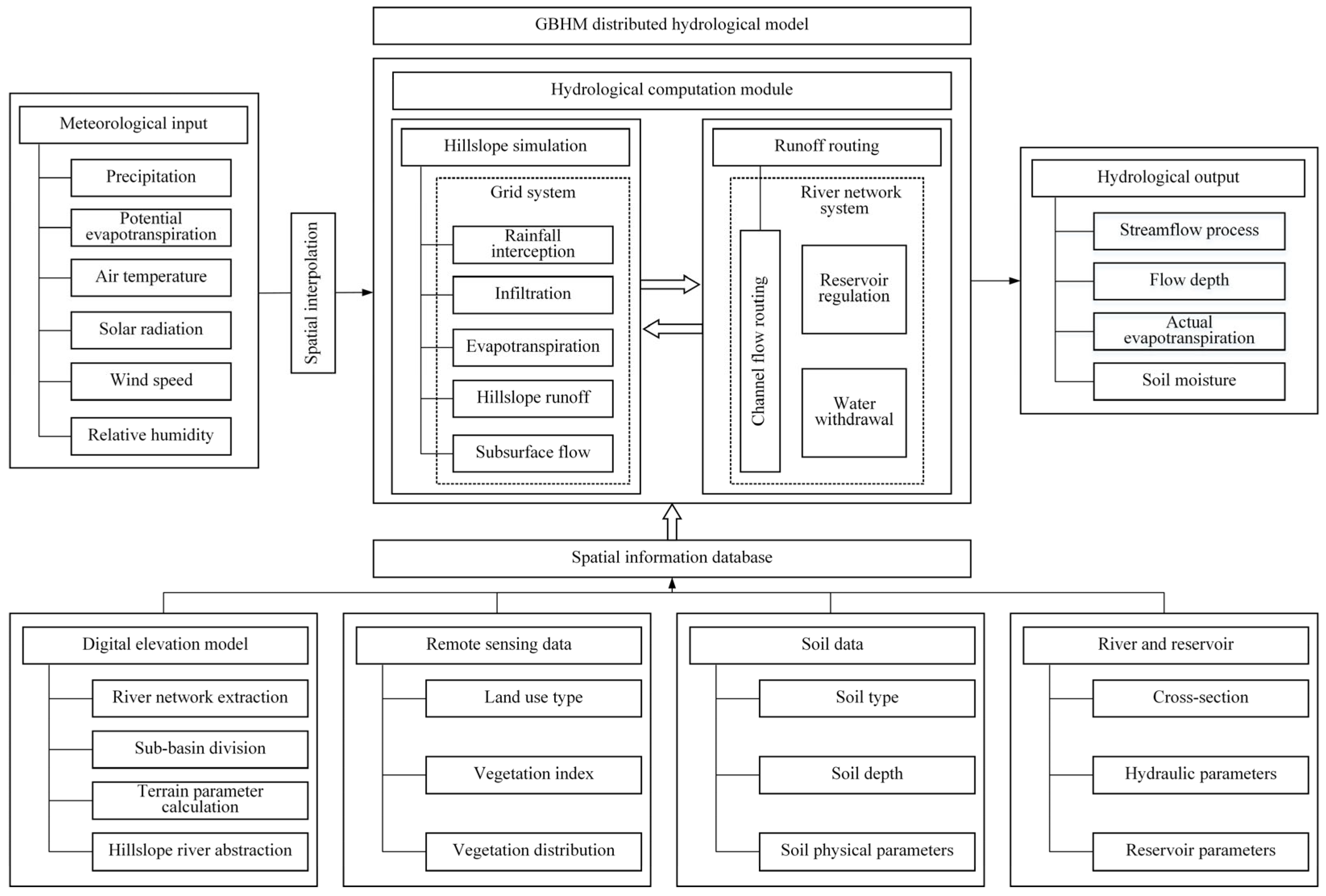
The GBHM model is a distributed hydrological model that uses hillslopes as its basic units. Built upon Digital Elevation Models (DEMs) and Geographic Information Systems (GISs), the model consists of four modules: spatial discretization, watershed hydrological computation, meteorological input, and hydrological output. The structure of the model is shown in Figure 4 [80,81,82]. Firstly, spatial discretization is performed using “hillslopes” as the basic units. Subsequently, based on topography, calculations of flow direction, river network generation, and sub-basin delineation are completed. Combined with spatial variability characteristics, the watershed is discretized into individual “hillslope” units, each assigned geospatial characteristic parameters. This forms a gridded system in the spatial domain of the watershed, constructing a hillslope–river network system for runoff generation and convergence.

3.4. Evaluation Index

The Nash-Sutcliffe efficiency coefficient (NSE), percentage bias (PBIAS), and the ratio of root mean square error to observed standard deviation (RSR) are used to evaluate the simulation accuracy of the rainfall-runoff model. The calculation methods are as follows:

$$NSE=1-\left[{\displaystyle \frac{{\displaystyle \sum _{i=1}^n{\left(Y_i^{obs}-Y_i^{sim}\right)}^2}}{{\displaystyle \sum _{i=1}^n{\left(Y_i^{obs}-Y^{mean}\right)}^2}}}\right],$$

(2)

$$PBIAS=\left[{\displaystyle \frac{{\displaystyle \sum _{i=1}^n\left(Y_i^{obs}-Y_i^{sim}\right)}}{{\displaystyle \sum _{i=1}^n{Y}_i^{obs}}}}\right]\times 100\%,$$

(3)

$$RSR={\displaystyle \frac{RMSE}{STDE{V}_{obs}}}=\left[{\displaystyle \frac{\sqrt{{\displaystyle \sum _{i=1}^n{\left(Y_i^{obs}-Y_i^{sim}\right)}^2}}}{\sqrt{{\displaystyle \sum _{i=1}^n{\left(Y_i^{obs}-Y_i^{mean}\right)}^2}}}}\right],$$

(4)

where $Y_i^{obs}$ represents the $i$-th observed value in the evaluation series, $Y_i^{sim}$ represents the $i$-th simulated value in the evaluation series, $Y^{mean}$ represents the average of the observed data in the evaluation series, and $n$ represents the total number of values in the evaluation series.

In addition, to better evaluate the model’s extreme value simulation performance, the extreme flow absolute percentage error coefficient (APE-2%) is introduced. APE-2% is an extreme value fitting evaluation method based on the absolute percentage error (APE), which considers the extreme flow values in the top 2% of the frequency distribution for calculation [30]. The calculation methods for the original APE and APE-2% are as follows:

$$APE={\displaystyle \frac{\left|Y_i^{sim}-Y_i^{obs}\right|}{Y_i^{obs}}}\times 100\%,$$

(5)

$$APE-2\%={\displaystyle \frac{{\displaystyle \sum _{i=1}^n\left|Y_i^{sim}-Y_i^{obs}\right|}}{{\displaystyle \sum _{i=1}^n{Y}_i^{obs}}}}\times 100\%$$

(6)

The closer APE-2% is to 0, the smaller the deviation in extreme flow simulation, indicating that the model can accurately simulate the characteristics of extreme flow.

4. Results and Discussion

The results proceed in three stages: GBHM baseline skill and peak bias; RRT/RC-RRT performance on long-sequence and extreme events; and RCGR improvements over both physical and data-driven baselines, highlighting peak-flow fidelity and generalization.

4.1. Analysis of Simulation Performance of Physically Based Model

Using the constructed GBHM model, we simulated the daily runoff process in the Xinanjiang Basin from 1970 to 2019, with 1970–1999 as the calibration period and 2000–2019 as the validation period. Figure 5 illustrates the observed and simulated daily runoff time series at the Tunxi, Yuliang, and Yuetan stations for both calibration and validation.

Table 1. GBHM model simulation results of runoff during the calibration and validation periods.

Stations	Daily Runoff Simulation Results
	Calibration Period (1970–1999)				Validation Period (2000–2019)
	NSE	PBIAS (%)	RSR	APE-2% (%)	NSE	PBIAS (%)	RSR	APE-2% (%)
Tunxi	0.85	3.94	0.39	24.84	0.81	8.28	0.43	22.44
Yuliang	0.83	−9.54	0.41	28.02	0.81	−2.98	0.43	24.25
Yuetan	0.76	−1.69	0.49	28.73	0.72	2.96	0.53	27.55

summarizes the model’s daily runoff simulation results at these representative stations during the two periods. Overall, the three stations exhibited satisfactory performance, achieving NSE values above 0.7, PBAIS within ±10%, and RSR below 0.6 during validation.

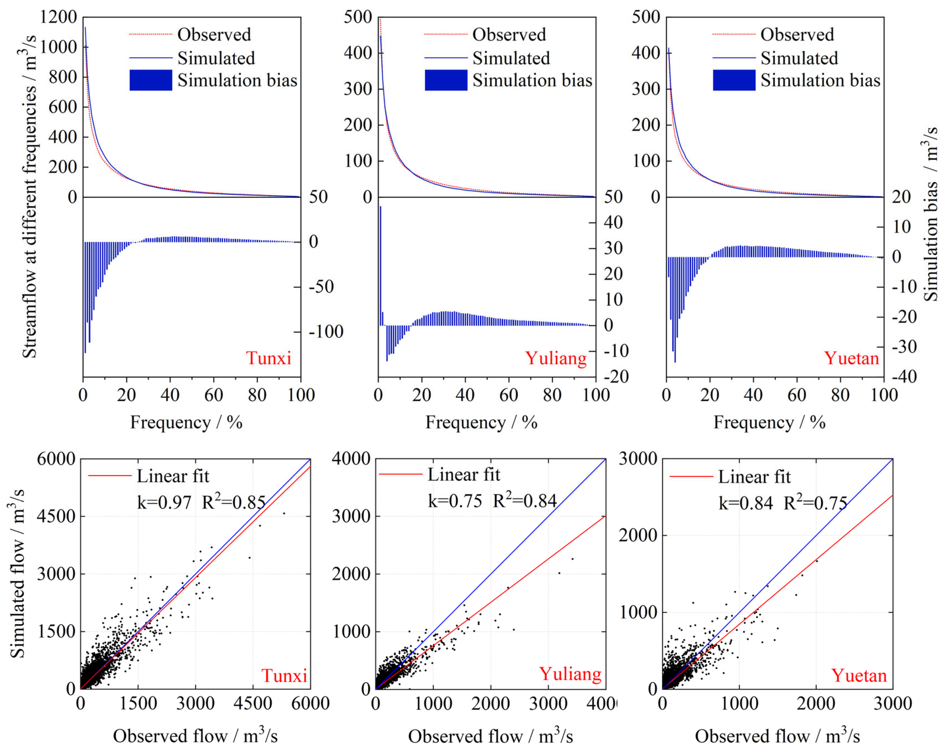
The model generally captures flood peak timing but tends to underestimate peak flows for certain events. Among the five largest floods at Tunxi Station (1994, 1996, 2006, 2008, and 2011), only the 2008 flood exhibited a relatively small average peak-flow error across the three stations (5.2%), whereas the remaining events ranged from 20.5% to 29.0%, mostly underestimations. As shown in Figure 6, high-flow underestimation is more evident at Yuliang and Yuetan Stations, where most simulated–observed flow points exceeding 1000 m³/s lie below the 1:1 reference line. From the flow duration curve and the flow difference bar charts at various frequencies, flows within the 20% threshold show larger overall deviations. When focusing on the 1% threshold, most flow discrepancies are positive, and the gap widens with higher flows, indicating that the GBHM model has difficulty accurately simulating extreme floods, frequently yielding underestimates. Moreover, the model’s relative errors for 18 extreme flood events ranged from 5.1% to 56.9% (averaging 31.3%), with four events exceeding 50%. These biases may stem from soil parameters derived from a global database that might lack regional applicability in the Xinanjiang Basin. In addition, physical process hydrological models require lengthy runtimes, time-consuming calibration, and considerable operator expertise, which complicates simultaneously ensuring accuracy for mid-to-low flows and extreme flows. Consequently, this study integrates the physical process model with a deep learning approach to refine runoff simulations based on preliminary calibration results.

4.2. Evaluation and Analysis of Data-Driven Model

(1)

Introducing a Time Window Mechanism for the Transformer Model

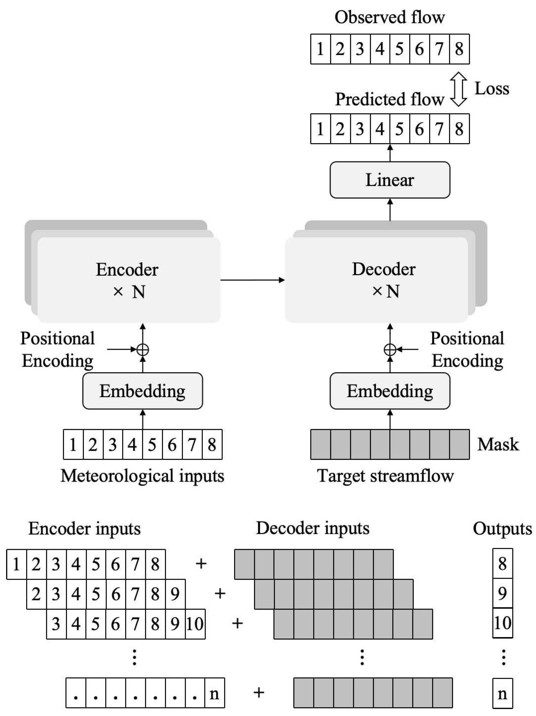
In the original Transformer architecture, the decoder masks the target flow to prevent the model from accessing true flow values during training, thereby ensuring error-based backpropagation. Autoregressive decoding suffers from error accumulation when predicting extended lead times, while non-autoregressive decoding, although accurate in short-term forecasts, relies on observed flow at each step and thus proves unsuitable for long-term predictions. Consequently, this study proposes a fully masked structure, named the Fully Masked Rainfall–Runoff Transformer (RRT) model, which omits explicit flow inputs in the encoder and uses only meteorological data to predict streamflow (Figure 7). By exploiting the relationship between meteorological sequences and flow, the approach avoids dependence on prior flow conditions and eliminates error accumulation, making it theoretically applicable to long-term flow simulations.

To ensure comparability with the GBHM model, the RRT model utilizes identical meteorological input variables, including daily precipitation, mean air temperature, mean atmospheric pressure, mean relative humidity, sunshine duration, and mean wind speed. The model outputs daily streamflow at three hydrological stations: Tunxi, Yuliang, and Yuetan. The RRT model was trained using data from 1972 to 2007, encompassing 12,783 valid daily records. The validation period spans from 2008 to 2012 (1827 days), and the testing period from 2014 to 2018 (1826 days). Certain years were excluded due to missing streamflow data at some stations. Consequently, the training, validation, and testing sets account for 78%, 11%, and 11% of the data, respectively. In addition, to mitigate overfitting during model training, an early stopping strategy was adopted. Specifically, model performance on the validation set was monitored during each training iteration, and training was terminated when no significant improvement in validation metrics was observed over multiple consecutive epochs. The model’s performance on the testing set was subsequently used as the primary basis for evaluating simulation accuracy and robustness.

Antecedent hydrometeorological conditions significantly influence flow forecasts. To ensure accuracy and robustness, the time window setting requires careful consideration during model development. While each prediction step necessitates sufficient meteorological data, excessive historical input can induce overfitting and weaken predictive performance. Therefore, this study evaluated five time window sizes—3, 5, 7, 14, and 21 days—when constructing the fully masked RRT model to determine the optimal structure. Despite applying the same early-stopping strategy, training variations often produced substantial deviations in testing when validation performance appeared optimal, indicating persistent overfitting. To achieve stable and reliable outcomes, multiple training iterations were performed under the same early-stopping conditions for each time window setting, and model snapshots were saved. The snapshot exhibiting the best evaluation metrics and most consistent predictive performance was selected as the optimal model for that time window.

Table 2. Simulation performance under different time window settings.

Time Window Size	Validation Period (2008–2012)				Test Period (2014–2018)
	NSE	RSR	PBIAS (%)	APE-2% (%)	NSE	RSR	PBIAS (%)	APE-2% (%)
3	0.74	0.51	24.2	33.46	0.72	0.53	16.88	29.42
5	0.77	0.48	7.89	32.79	0.76	0.49	1.48	30.73
7	0.79	0.46	1.68	30.07	0.79	0.46	−5.60	24.46
14	0.79	0.46	0.19	27.36	0.75	0.50	−3.26	31.78
21	0.80	0.44	−4.37	31.03	0.72	0.53	−12.08	30.21

presents the simulation results for different time windows. When the time window is set to 3 days, the RRT model fails to incorporate sufficient antecedent meteorological information, leading to unsatisfactory performance, with PBIAS reaching 24.2% in the validation period. At a 7-day window, the model achieves optimal results, exhibiting similar performance between validation and training, with NSE and RSR reaching 0.79 and 0.46, respectively, and PBIAS within 6%. The model thus demonstrates both accuracy and stability, while the 5-day window ranks second in performance. Consequently, 4–6 days of historical meteorological data appear the most influential in runoff forecasting using meteorological inputs alone. When the window extends to 14 days or more, training performance declines relative to the 5-day and 7-day windows, indicating overfitting caused by excessive data. Moreover, windows of at least 14 days markedly slow training and increase memory demands (approximately 15 GB at 14 days). Therefore, in subsequent analyses, the fully masked RRT model employs a 7-day window.

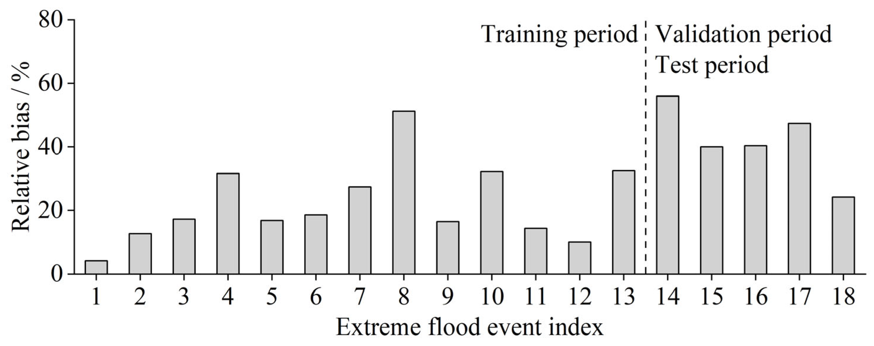
Figure 8 illustrates the runoff predictions for a 7-day window, revealing comparable performance in both validation and testing. Although mid-to-low flow fitting is satisfactory, high flows are notably underestimated. For instance, on 4 June 2008, simulated flow is 1439 m³/s versus an observed 3420 m³/s, yielding a 58% deviation; on 8 June 2011, the model underestimates at 2507 m³/s against 4410 m³/s, a 43% error. Nevertheless, extreme-flow simulations in the testing period outperform those in the validation period (APE-2% = 24.46%), partly because peak flows in the test set are generally smaller. However, underestimation of peak flows remains frequent. Figure 9 shows the model’s performance for extreme flood events, with relative errors ranging from 4.1% to 56.0% and an average of 27.4%. Two extreme events exceed 50% error. Notably, during training, the mean error for extreme events is lower (21.9%) but still considerable. This result arises from the limited number of extreme event samples relative to the full dataset, making them challenging to predict precisely.

Although some discrepancy persists in extreme flood simulations, the model achieves an overall “good” performance rating, accurately tracking runoff variations and surpassing traditional distributed hydrological models for low-flow conditions. Future work may focus on refining peak-flow estimates to enhance simulation accuracy.

(2)

Introducing a Runoff Classification Mechanism for the RRT Model

Although the fully masked RRT model has been successfully applied to long-term runoff forecasting, it remains challenging to simulate extreme flow events accurately. Because extreme events occur infrequently in the training dataset, they are underrepresented, leading to systematic underestimation of these rare occurrences in actual forecasts. To address this limitation, we adopt a classification-based approach in which meteorological inputs associated with low-to-moderate flows, high flows, and extremely high flows are categorized into three separate datasets. Each dataset is then used to train an RRT model independently.

For classification, we modify the Transformer model to support a cross-entropy loss function and one-hot encoded labels, where [1, 0, 0], [0, 1, 0], and [0, 0, 1] correspond to low-to-moderate, high, and extremely high flows, respectively. A Softmax activation function outputs the probabilities for each category, and classification accuracy measures the proportion of correctly categorized samples. Based on historical flow data and frequency analysis, we classify flows below the 80th percentile, between the 80th and 95th percentiles, and above the 95th percentile into three subsets, along with their corresponding meteorological sequences. To rigorously evaluate model performance, we split each subset into training (80%), validation (10%), and testing (10%) sets. Training ceases once the validation accuracy plateaus for multiple iterations, and the final model is assessed using the test set.

Classification results are shown in

Table 3. Performance of the Transformer-based classification model.

Category	Accuracy (%)
	Training	Validation	Test
Medium–low flow	99.8	97.8	98.5
High flow	98.9	98.6	95.4
Extreme flow	97.7	91.0	92.0
Overall	99.4	97.6	97.5

. The Transformer model demonstrates strong classification performance, achieving up to 99.4% accuracy on the training set and 97.5% on both validation and testing, underscoring its robustness and stability. Even the relatively scarce “extremely high” flow category exceeds 90% accuracy. Using the classification outcomes, we partition the data for the RRT model. To ensure each time step has sufficient antecedent hydrometeorological inputs, a sliding-window approach is employed. After partitioning, each subset is trained using the fully masked RRT model. The same method is applied to the validation and testing sets, and predictions from all three models are merged according to their original sequence to assess overall performance.

As shown in

Table 4. Performance of the fully masked RRT model based on runoff classification.

Station	Validation Period				Test Period
	NSE	RSR	PBIAS (%)	APE-2% (%)	NSE	RSR	PBIAS (%)	APE-2% (%)
Tunxi	0.91	0.29	3.96	23.80	0.85	0.39	−0.14	21.53
Yuliang	0.87	0.35	−4.92	27.53	0.77	0.48	−5.58	29.08
Yuetan	0.88	0.34	3.26	23.40	0.80	0.46	−0.46	24.63

, the RRT model with runoff classification (RC-RRT) yields favorable results during both validation and testing, with NSE, RSR, and PBIAS reaching 0.91, 0.29, and 3.96%, respectively, in validation. Figure 10 indicates reliable fitting in the low-to-moderate flow range and reasonable peak-flow forecasts between 2008 and 2011, although a substantial error persists for the June 2011 peak (observed 4410 m³/s vs. modeled 3032 m³/s). While this 31% discrepancy improves upon the 43% error from the fully masked RRT model, additional refinements are needed. The limited training samples for such high flows—only one event since 1970 exceeding this level (5310 m³/s at Tunxi Station in July 1996)—suggests constraints in data-driven extrapolation. Nonetheless, the classification-based approach achieves an overall “good” performance, particularly enhancing peak-flow simulation accuracy.

By comparing the simulation performance of the fully masked RRT model with its runoff-classification-based variant during the testing period (Figure 11), the classification mechanism significantly improves peak-flow predictions without compromising mid-to-low flow accuracy. Specifically, APE-2% drops from 24.5% to 21.5%, and flow deviations above the 90th percentile decrease from 26% to 22%, effectively mitigating underestimation. Figure 12 shows the model’s performance on extreme flood events, with errors ranging between 0.4% and 40.9% (averaging 14.7%). Except for a 41% error in June 2016, the relative error of all other events remains under 30%. Although the model’s errors in the validation and testing phases surpass those in training, the classification step reduces the average relative error from 41.6% to 26.5%, indicating further room for improvement.

While the RC-RRT model demonstrates strong performance overall, a closer look at the 2008–2019 period in both validation and testing reveals declining performance in later years, with NSE decreasing from 0.91 to 0.85. This reduction may be tied to global climate change and human activities altering the underlying hydrometeorological relationships that the RRT model, relying solely on meteorological data, struggles to capture fully. Consequently, the study couples the model with a physical process hydrological framework to leverage its ability to represent changes in underlying surface conditions, thereby enhancing simulation stability.

4.3. Simulation Performance and Analysis of the Coupled Model

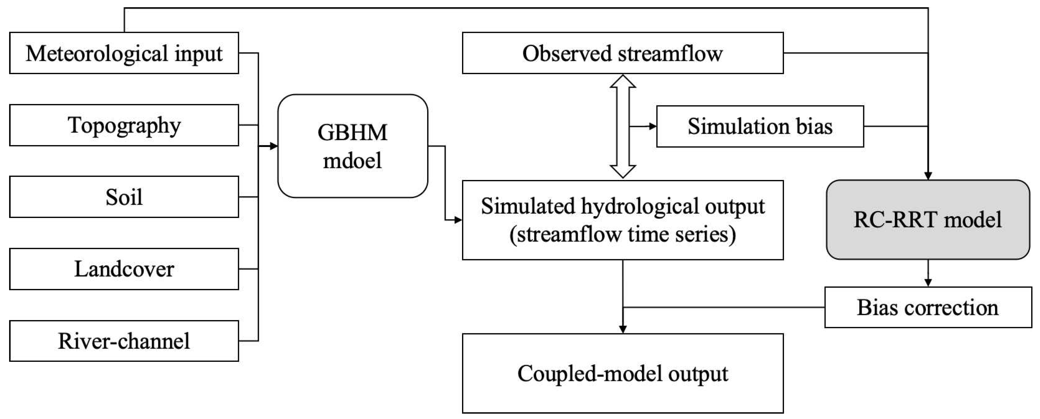
Due to the limitations of data accuracy and theoretical assumptions, simulation outputs from physically based models inevitably exhibit biases. However, these biases often display autocorrelation characteristics. To enhance predictive accuracy, machine learning models can be employed to model the residuals. In this approach, the observed streamflow is expressed as the sum of the physically based model output and a learnable error component. This residual correction strategy effectively mitigates systematic errors and improves overall simulation performance, as illustrated in Figure 13.

As shown in

Table 5. Performance of the coupled model based on runoff classification and bias correction.

Station	Validation Period				Test Period
	NSE	RSR	PBIAS (%)	APE-2% (%)	NSE	RSR	PBIAS (%)	APE-2% (%)
Tunxi	0.93	0.27	−0.46	20.97	0.93	0.27	−0.50	19.07
Yuliang	0.89	0.33	1.38	27.57	0.87	0.36	4.82	24.17
Yuetan	0.91	0.29	0.24	25.02	0.90	0.32	−3.37	19.71

, the GBHM–RRT coupled model based on runoff classification and bias correction (RCGR) substantially outperforms the RC-RRT model, boosting NSE, RSR, and APE-2% at Tunxi Station from 0.82, 0.43, and 26.89% to 0.93, 0.27, and 19.07%, respectively, while maintaining PBIAS below 0.5%. Moreover, similar performance on validation and testing underscores the RCGR model’s stability and reliability.

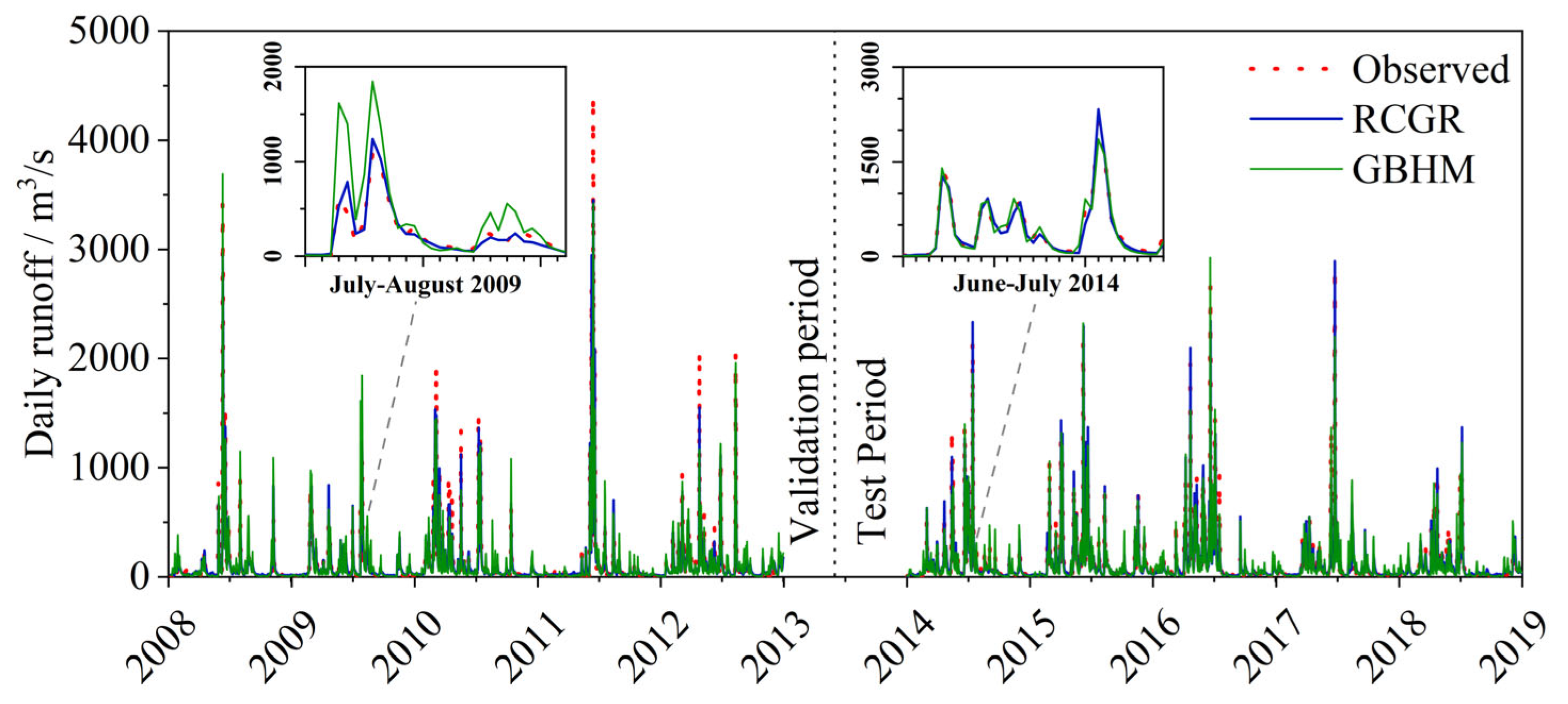
Since the GBHM model simulations are categorized only into calibration and validation periods, data from 2008 to 2018 were extracted for comparison with the RCGR-coupled model. After applying the RC-RRT model to learn and correct the simulation errors of GBHM, model performance improved significantly. For instance, at Tunxi Station during the testing period, the NSE increased from 0.86 to 0.93, RSR decreased from 0.37 to 0.27, and PBIAS improved from −4.49% to −0.50%. While the APE-2% for extreme flow simulation remained comparable, the average APE-2% across the three stations slightly decreased from 22.78% to 20.98%. As illustrated in Figure 14, the RCGR -coupled model outperformed the standalone GBHM model, with the RRT component effectively correcting most peak-flow biases in GBHM, such as the overestimation during July–August 2009 and the underestimation in June–July 2014. However, for certain extreme events (e.g., June 2008 and June 2011), the correction capability of the RC-RRT model was limited.

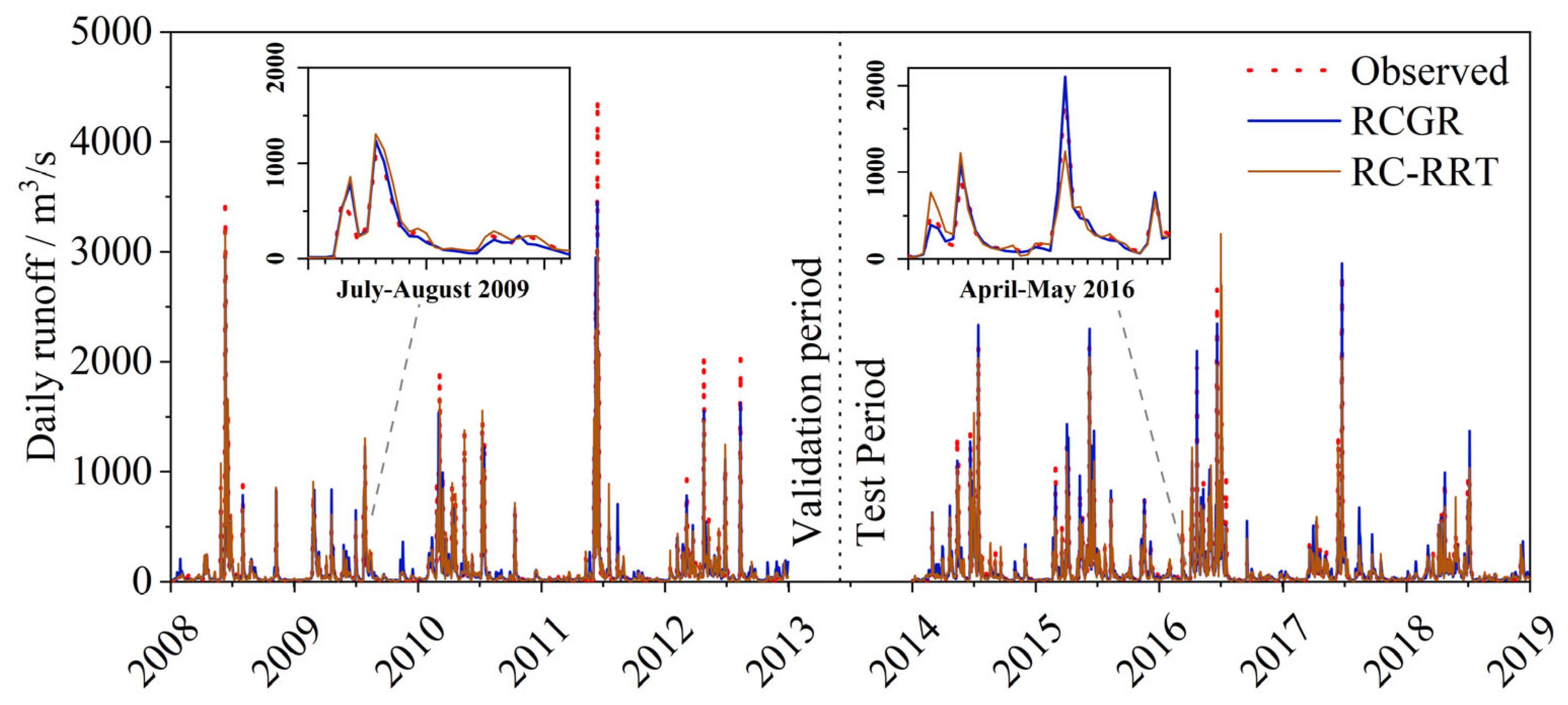
Figure 15 contrasts the RCGR model against the RC-RRT model. Their validation performance differs marginally (NSE of 0.93 versus 0.91 and peak-flow error within a 3% gap). Both capture most flow variations and peaks reliably (e.g., July–August 2009). However, the RCGR model excels during testing, particularly for the April–May 2016 peak, around 1950 m³/s. Although the RC-RRT approach significantly enhances peak simulations, it remains constrained by the inherent generalization limits of data-driven methods and incurs a 35% error. In contrast, the coupled approach reduces this error to under 10%, reflecting its superior modeling capabilities.

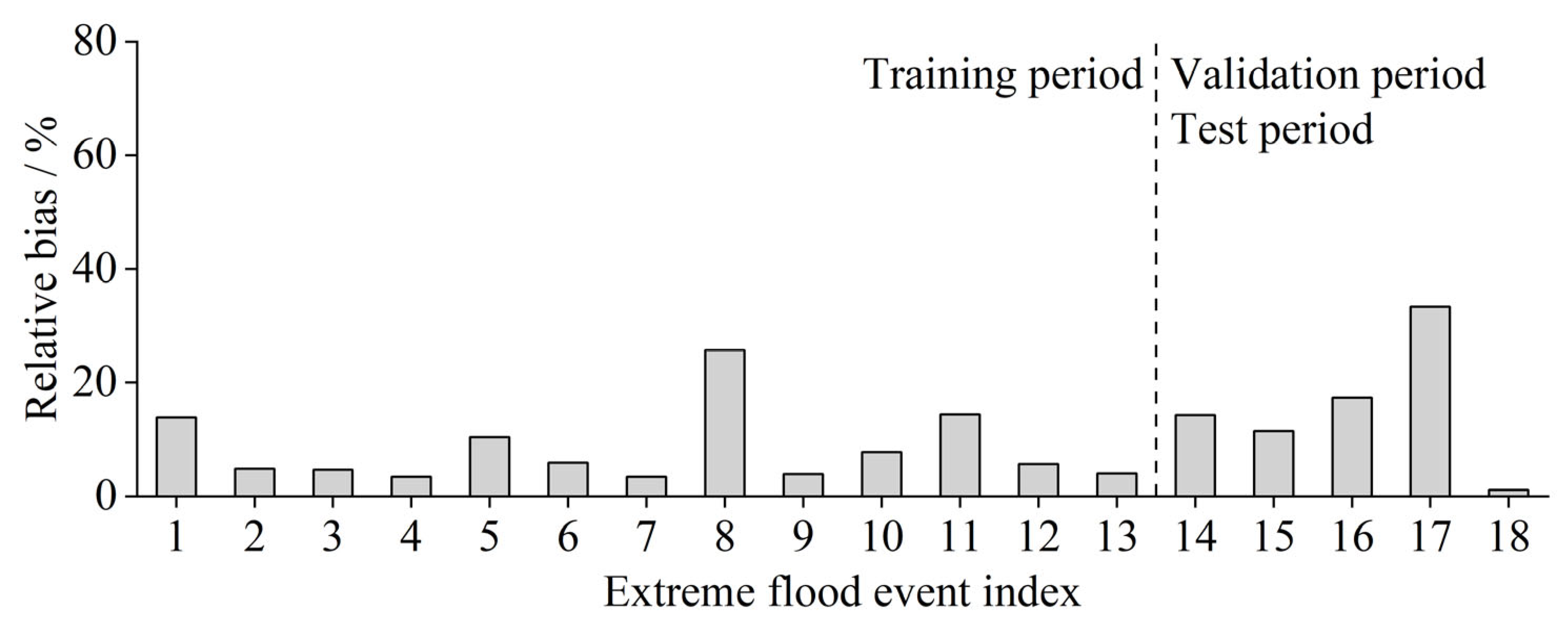
Figure 16 exhibits the RCGR model’s extreme flood simulation, with errors ranging from 1.1% to 33.3% (mean 10.3%). Aside from deviations of 25.7% and 33.3% in July 1996 and June 2016, all other extreme events remain under 20% error. While training errors stand at 8.3%, validation and testing errors increase to 15.5%, still markedly lower than those in standalone data-driven models, illustrating improved stability under coupling. By incorporating GBHM outputs as an additional input, the coupled model benefits from the strong correlation between GBHM and observed flows, helping alleviate overfitting and thereby extending temporal generalization. Validation and testing at Yuliang Station yield NSE values of 0.89 and 0.87, respectively, while Yuetan Station achieves 0.91 and 0.90, confirming that the coupled model’s generalization surpasses that of the RC-RRT model.

4.4. Discussion

This section synthesizes the main findings and benchmarks them against standard baselines, including physically based (GBHM, XAJ, SWAT) and data-driven (ANN, LSTM, WLSTM, BiLSTM, RC-RRT) models.

(1)

Comparison with physically based hydrological models

A comparative analysis was conducted between the widely adopted XAJ model and SWAT models in the XRB region [66,83], as summarized in

Table 6. Comparison of simulation performance between the coupled model and the physically based hydrological model.

Model	Station	Validation Period				Test Period
		NSE	RSR	PBIAS (%)	APE-2% (%)	NSE	RSR	PBIAS (%)	APE-2% (%)
GBHM	Tunxi	0.81	0.44	−11.15	24.46	0.86	0.37	−4.49	19.12
	Yuliang	0.81	0.44	2.52	26.22	0.82	0.43	4.23	22.88
	Yuetan	0.74	0.51	−3.43	30.20	0.77	0.48	0.93	26.34
XAJ	Tunxi	0.84	0.40	−12.55	26.98	0.89	0.33	−9.41	14.91
	Yuliang	0.76	0.49	−1.25	32.90	0.72	0.53	−10.56	29.81
	Yuetan	0.85	0.39	−16.44	23.37	0.88	0.346	−16.83	21.97
SWAT	Tunxi	0.79	0.45	−0.08	40.95	0.73	0.52	2.18	33.90
	Yuliang	0.78	0.47	−15.25	26.40	0.74	0.51	−19.10	21.51
	Yuetan	0.72	0.53	4.80	45.37	0.64	0.60	6.01	44.16
RC-RRT	Tunxi	0.91	0.29	3.96	23.80	0.85	0.39	−0.14	21.53
	Yuliang	0.87	0.35	−4.92	27.53	0.77	0.48	−5.58	29.08
	Yuetan	0.88	0.34	3.26	23.40	0.80	0.46	−0.46	24.63
RCGR	Tunxi	0.94	0.24	−4.19	12.73	0.95	0.23	−2.52	10.63
	Yuliang	0.94	0.26	6.16	12.77	0.92	0.29	4.49	14.75
	Yuetan	0.93	0.27	−3.75	15.94	0.91	0.31	−4.25	15.47

. Across all evaluation periods, the RCGR-coupled model consistently outperformed standalone physically based hydrological models and data-driven models in terms of NSE, RSR, PBIAS, and APE-2%. The NSE improved from 0.70 to 0.85 to above 0.90, and PBIAS was controlled within 7% at all stations. Additionally, the coupled model demonstrated comparable performance during the validation and testing phases, indicating strong model stability.

Compared with the GBHM model, the RCGR model achieved over a 10% increase in NSE, particularly at Yuetan Station, where the relatively weaker performance of GBHM (NSE = 0.74) was significantly enhanced to 0.93 through deep learning of meteorological-hydrological relationships. When benchmarked against the standalone data-driven RRT model, both models exhibited similar performance during the validation period. However, in the testing phase, the RRT model showed slightly reduced accuracy at Tunxi and Yuliang stations. This suggests that data-driven models rely heavily on learned correlations within meteorological-hydrological sequences, which remain relatively stable over short periods. Under the dual influences of climate change and anthropogenic activities, these correlations may shift, and data-driven models—limited by the scope of meteorological input—fail to capture such changes, leading to diminished predictive performance and reduced generalization capabilities in extended forecasts. In contrast, coupling with a physically based distributed model mitigates this limitation, significantly enhancing model robustness.

For extreme flood event simulations, Figure 17 illustrates the comparative error analysis between the coupled model and standalone models. The SWAT model yielded relative errors ranging from 2.7% to 77.8%, with an average of 30.1%, while the Xin’anjiang model showed a range of 5.8% to 72.7%, averaging 28.4%. Both models exhibited consistent performance during calibration (events 1–10) and validation periods (events 11–18). Notably, the GBHM model maintained a stable average relative error of 31.4% and 31.2% for the two periods, attributed to its capacity to account for meteorological and land use changes. Although both the RC-RRT and RCGR models showed some discrepancies between training (events 1–13) and validation/testing (events 14–18) phases, the coupled model significantly reduced the variability in extreme event simulation accuracy across periods. Moreover, it preserved the robustness of the GBHM model under changing environmental conditions while achieving enhanced precision in simulating extreme hydrological events.

Physically based hydrological models demonstrate high accuracy and stability in simulating average hydrological conditions; however, they often exhibit considerable deviations when modeling extreme events. In contrast, data-driven models are adept at uncovering latent relationships among variables, granting them a significant advantage in simulating extremes. Therefore, integrating physically based models with data-driven approaches offers a promising strategy for enhancing the accuracy of extreme hydrological event simulations.

(2)

Comparison with data-driven models

Several widely used machine learning models for rainfall–runoff simulation were selected for comparison, including the Artificial Neural Network (ANN) [84], Long Short-Term Memory network (LSTM) [85], Wavelet-LSTM model (WLSTM) [74,86], and Bidirectional LSTM (BiLSTM) [87]. Given that the primary objective of this study is to achieve long-sequence runoff simulation, all data-driven models were developed following the architectural design of the fully masked RRT model to ensure consistency in input data structure. A temporal window of 7 days was adopted, where meteorological data over each 7-day window were used to predict the runoff on the 7th day. The predicted runoff values of each 7th day were then concatenated to form the complete forecast sequence.

To ensure consistency across models, the dataset was partitioned identically to the Transformer model, with the training, validation, and testing periods accounting for 78%, 11%, and 11% of the total dataset, respectively. Model hyperparameters were optimized through manual trial-and-error, and the early stopping strategy was aligned with that of the Transformer, where training was terminated once the validation NSE showed no significant improvement after successive iterations. The iteration yielding the best validation NSE was selected as the final model configuration. Acknowledging the stochastic nature of model training, each model underwent 500 independent runs, and the best-performing result was adopted to represent the final model outcome. A detailed summary of model performance at the Tunxi station is presented in

Table 7. Comparative simulation performance of various data-driven models.

Model	Validation Period				Test Period
	NSE	RSR	PBIAS (%)	APE-2% (%)	NSE	RSR	PBIAS (%)	APE-2% (%)
RC-RRT	0.79	0.46	1.68	30.07	0.79	0.46	−5.60	24.46
RCGR	0.94	0.24	−4.19	12.73	0.95	0.23	−2.52	10.63
ANN	0.78	0.47	7.53	32.79	0.72	0.53	−1.31	24.34
LSTM	0.73	0.52	−6.50	28.86	0.68	0.56	−9.56	27.59
WLSTM	0.77	0.48	5.51	32.26	0.72	0.53	1.96	32.23
BiLSTM	0.76	0.49	−3.39	39.13	0.71	0.54	−10.81	35.10

.

In both the validation and testing phases, aside from the RCGR coupled model, the RC-RRT model and other data-driven approaches exhibited comparable performance, with NSE values generally exceeding 0.7 and PBIAS maintained at relatively low levels. This indicates that the RC-RRT model performs on par with widely adopted and validated models such as ANN, LSTM, and their variants in long-sequence rainfall-runoff simulation. The simulation errors for extreme flood events, as illustrated in Figure 18, show that the relative errors for ANN, LSTM, WLSTM, and BiLSTM models range from 0.7 to 45.7%, 2.3–40.8%, 0.8–41.4%, and 7.4–60.6%, respectively, with corresponding average errors of 14.5%, 15.4%, 16.0%, and 27.0%. These results suggest that, excluding BiLSTM, the extreme event simulation accuracy of data-driven models is generally comparable to that of the RRT model, with no significant performance disparity. Although the BiLSTM model performs well overall, its accuracy in simulating extreme events remains suboptimal. The similar performance of various data-driven models in extreme event scenarios implies that model architecture exerts limited influence on simulation accuracy under such conditions. Instead, the primary limitation stems from the scarcity of extreme event samples within the overall training dataset. This is further corroborated by the observation that the RC-RRT model, which incorporates runoff classification, achieved over a 50% improvement in extreme event simulation accuracy compared to the fully masked RRT model. Additionally, when comparing the simulation accuracy across training, validation, and testing periods, standalone data-driven models exhibit notable discrepancies in extreme event performance, highlighting limited model robustness and generalizability. In contrast, the RCGR coupled model demonstrates consistent performance across all periods, delivering both high and stable accuracy in simulating extreme hydrological events.

5. Conclusions

This work enhances the Transformer model to be more appropriate for long-term runoff forecasting and extreme flood event simulation. Meanwhile, a distributed hydrological model GBHM is established based on the geomorphological characteristics of watersheds, and a coupled framework of the distributed model and a data-driven hydrological model is provided. The framework incorporates an error correction mechanism for improved overall simulation accuracy and extreme event performance. Comparative simulations with physically based and data-driven models provide the following main conclusions:

(1)

The GBHM model, constructed based on watershed geomorphology, demonstrates generally reliable simulation performance, accurately capturing the timing of flood peaks in most events. However, it tends to significantly underestimate peak discharges during some extreme flood events, with an average relative error of approximately 31.3%. This underestimation is likely attributable to the temporal resolution limitations of historical rainfall data; specifically, hourly rainfall inputs were interpolated from daily data, potentially leading to rainfall intensity biases. Consequently, the model’s performance is constrained by input data quality and parameter generalization strategies inherent in physically based models.

(2)

The Transformer model, leveraging its encoder–decoder structure and multi-head attention mechanism, enhances runoff prediction accuracy and stability. Comparative experiments on the fully masked RRT model with varying sliding window lengths reveal that a 7-day window yields optimal performance in the XRB. Incorporating a runoff classification module further improves prediction, achieving NSE values of 0.87–0.91 in the validation phase and 0.77–0.85 in testing, with APE-2% maintained below 30%. Simulation errors for extreme events are substantially reduced to 14.7%. However, the results indicate performance degradation under changing environmental conditions when the model relies solely on meteorological inputs, which is an issue more pronounced in long-term runoff forecasting.

(3)

The enhanced RRT model predicts runoff using only meteorological inputs, independent of observed or previously predicted flow values at each time step, thereby eliminating error accumulation. This design supports long-sequence runoff forecasting. Its multi-head self-attention mechanism enables the model to capture complex spatiotemporal relationships between meteorological and runoff sequences and to establish long-range dependencies unconstrained by sliding windows. This capability allows the model to learn underlying patterns across the entire input sequence, improving prediction robustness and accuracy. Furthermore, the model’s parallel processing architecture enhances computational efficiency, making it suitable for hydrological forecasting across diverse climatic and geographical settings.

(4)

The proposed RCGR coupled model—built on an error correction framework—significantly outperforms the standalone GBHM model in terms of simulation accuracy and generalization. It addresses the limited extrapolative capacity of data-driven models under changing environmental conditions. By enriching the data-driven component with additional relevant information, the best-performing coupled model achieves NSE values of 0.91–0.95. The relative errors in extreme event simulations range from 1.5% to 26.3%, with an average of 9.7%, and 60% of events exhibit simulation errors below 10%, demonstrating a marked improvement in the accuracy of extreme flood simulations.

Taken together, this study indicates that the RCGR coupling sustains skill from short-sequence to decadal-scale prediction while improving peak-flow fidelity and robustness under changing conditions (NSE up to 0.95; mean extreme event error ≈10%). RC-RRT provides a lightweight alternative for applications when simplicity and computing budgets dominate, whereas GBHM alone remains suitable when process interpretability and scenario analysis are central. The workflow is readily portable where a distributed/semi-distributed model can be calibrated and daily hydro-meteorological records are available; basin-specific tuning of flow percentile thresholds, time window length, and the residual bias module is typically sufficient for transfer.

Although the current GBHM–RRT coupling relies solely on an error correction mechanism, considerable gains have been achieved. Building on prior coupling model research, future work should investigate the modular replacement of GBHM subcomponents—such as evapotranspiration, interception, and infiltration calculations—to evaluate their impact on extreme event simulation accuracy. Additionally, applying the coupling framework to higher temporal resolutions (e.g., hourly scale) and assessing its performance under such conditions remain important directions for further study.

References

1. Tabari, H. Climate Change Impact on Flood and Extreme Precipitation Increases with Water Availability. Sci. Rep. 2020, 10, 13768. [Google Scholar] [CrossRef]
2. Kreibich, H.; Van Loon, A.F.; Schröter, K.; Ward, P.J.; Mazzoleni, M.; Sairam, N.; Abeshu, G.W.; Agafonova, S.; AghaKouchak, A.; Aksoy, H.; et al. The Challenge of Unprecedented Floods and Droughts in Risk Management. Nature 2022, 608, 80–86. [Google Scholar] [CrossRef]
3. Masson-Delmotte, V.; Zhai, P.; Pirani, A.; Connors, S.L.; Péan, C.; Berger, S.; Caud, N.; Chen, Y.; Goldfarb, L.; Gomis, M.; et al. Climate Change 2021: The Physical Science Basis; Contribution of Working Group I to the Sixth Assessment Report of the Intergovernmental Panel on Climate Change; Cambridge University Press: Cambridge, UK, 2021; Volume 2, p. 2391. [Google Scholar]
4. Wasko, C.; Nathan, R. Influence of Changes in Rainfall and Soil Moisture on Trends in Flooding. J. Hydrol. 2019, 575, 432–441. [Google Scholar] [CrossRef]
5. Liu, Z.; Yang, H.; Wei, X.; Liang, Z. Spatiotemporal Variation in Extreme Precipitation in Beijiang River Basin, Southern Coastal China, from 1959 to 2018. J. Mar. Sci. Eng. 2023, 11, 73. [Google Scholar] [CrossRef]
6. Mendelsohn, R.; Emanuel, K.; Chonabayashi, S.; Bakkensen, L. The Impact of Climate Change on Global Tropical Cyclone Damage. Nat. Clim. Change 2012, 2, 205–209. [Google Scholar] [CrossRef]
7. Sharafati, A.; Pezeshki, E. A Strategy to Assess the Uncertainty of a Climate Change Impact on Extreme Hydrological Events in the Semi-Arid Dehbar Catchment in Iran. Theor. Appl. Climatol. 2020, 139, 389–402. [Google Scholar] [CrossRef]
8. Tan, L.; Qi, J.; Marek, G.W.; Zhang, X.; Ge, J.; Sun, D.; Li, B.; Feng, P.; Li Liu, D.; Li, B.; et al. Assessing the Impacts of Extreme Precipitation Projections on Haihe Basin Hydrology Using an Enhanced SWAT Model. J. Hydrol. Reg. Stud. 2025, 58, 102235. [Google Scholar] [CrossRef]
9. Li, M.; Yang, D.; Hou, J.; Xiao, P.; Xing, X. Distributed Hydrological Model of Heilongjiang River Basin. J. Hydroelectr. Eng. 2021, 40, 65–75. [Google Scholar]
10. Zhang, C.; Wu, C.; Peng, Z.; Kuai, S.; Zhang, S. Synergistic Effects of Changes in Climate and Vegetation on Basin Runoff. Water Resour. Manag. 2022, 36, 3265–3281. [Google Scholar] [CrossRef]
11. Zhang, X.; Xu, Y.-P.; Fu, G. Uncertainties in SWAT Extreme Flow Simulation under Climate Change. J. Hydrol. 2014, 515, 205–222. [Google Scholar] [CrossRef]
12. Mei, Z.; Peng, T.; Chen, L.; Singh, V.P.; Yi, B.; Leng, Z.; Gan, X.; Xie, T. Coupling SWAT and LSTM for Improving Daily Streamflow Simulation in a Humid and Semi-Humid River Basin. Water Resour. Manag. 2024, 39, 397–418. [Google Scholar] [CrossRef]
13. Hinton, G.E.; Salakhutdinov, R.R. Reducing the Dimensionality of Data with Neural Networks. Science 2006, 313, 504–507. [Google Scholar] [CrossRef]
14. Sit, M.; Demiray, B.Z.; Xiang, Z.; Ewing, G.J.; Sermet, Y.; Demir, I. A Comprehensive Review of Deep Learning Applications in Hydrology and Water Resources. Water Sci. Technol. 2020, 82, 2635–2670. [Google Scholar] [CrossRef]
15. Noble, W.S. What Is a Support Vector Machine? Nat. Biotechnol. 2006, 24, 1565–1567. [Google Scholar] [CrossRef] [PubMed]
16. Song, Y.Y.; Lu, Y. Decision Tree Methods: Applications for Classification and Prediction. Shanghai Arch. Psychiatry 2015, 27, 130. [Google Scholar] [PubMed]
17. Breiman, L. Random Forests. Mach. Learn. 2001, 45, 5–32. [Google Scholar] [CrossRef]
18. Behzad, M.; Asghari, K.; Eazi, M.; Palhang, M. Generalization Performance of Support Vector Machines and Neural Networks in Runoff Modeling. Expert Syst. Appl. 2009, 36, 7624–7629. [Google Scholar] [CrossRef]
19. Ghumman, A.; Ghazaw, Y.M.; Sohail, A.; Watanabe, K. Runoff Forecasting by Artificial Neural Network and Conventional Model. Alex. Eng. J. 2011, 50, 345–350. [Google Scholar] [CrossRef]
20. Hu, C.; Wu, Q.; Li, H.; Jian, S.; Li, N.; Lou, Z. Deep Learning with a Long Short-Term Memory Networks Approach for Rainfall-Runoff Simulation. Water 2018, 10, 1543. [Google Scholar] [CrossRef]
21. Yamashita, R.; Nishio, M.; Do, R.K.G.; Togashi, K. Convolutional Neural Networks: An Overview and Application in Radiology. Insights Imaging 2018, 9, 611–629. [Google Scholar] [CrossRef]
22. Sherstinsky, A. Fundamentals of Recurrent Neural Network (RNN) and Long Short-Term Memory (LSTM) Network. Phys. D Nonlinear Phenom. 2020, 404, 132306. [Google Scholar] [CrossRef]
23. Chen, S.; Ren, M.; Sun, W. Combining Two-Stage Decomposition Based Machine Learning Methods for Annual Runoff Forecasting. J. Hydrol. 2021, 603, 126945. [Google Scholar] [CrossRef]
24. Mohammadi, B. A Review on the Applications of Machine Learning for Runoff Modeling. Sustain. Water Resour. Manag. 2021, 7, 98. [Google Scholar] [CrossRef]
25. Vaswani, A.; Shazeer, N.; Parmar, N.; Uszkoreit, J.; Jones, L.; Gomez, A.N.; Kaiser, Ł.; Polosukhin, I. Attention Is All You Need. Adv. Neural Inf. Process. Syst. 2017, 30, 5998–6008. [Google Scholar]
26. Kuratov, Y.; Arkhipov, M. Adaptation of Deep Bidirectional Multilingual Transformers for Russian Language. arXiv 2019, arXiv:1905.07213. [Google Scholar] [CrossRef]
27. Ismail Fawaz, H.; Forestier, G.; Weber, J.; Idoumghar, L.; Muller, P.-A. Deep Learning for Time Series Classification: A Review. Data Min. Knowl. Discov. 2019, 33, 917–963. [Google Scholar] [CrossRef]
28. Zhou, H.; Zhang, S.; Peng, J.; Zhang, S.; Li, J.; Xiong, H.; Zhang, W. Informer: Beyond Efficient Transformer for Long Sequence Time-Series Forecasting. In Proceedings of the AAAI Conference on Artificial Intelligence; AAAI Press: Washington, DC, USA, 2021; Volume 35, pp. 11106–11115. [Google Scholar] [CrossRef]
29. Liu, C.; Liu, D.; Mu, L. Improved Transformer Model for Enhanced Monthly Streamflow Predictions of the Yangtze River. IEEE Access 2022, 10, 58240–58253. [Google Scholar] [CrossRef]
30. Yin, H.; Guo, Z.; Zhang, X.; Chen, J.; Zhang, Y. RR-Former: Rainfall-Runoff Modeling Based on Transformer. J. Hydrol. 2022, 609, 127781. [Google Scholar] [CrossRef]
31. Li, W.; Liu, C.; Xu, Y.; Niu, C.; Li, R.; Li, M.; Hu, C.; Tian, L. An Interpretable Hybrid Deep Learning Model for Flood Forecasting Based on Transformer and LSTM. J. Hydrol. Reg. Stud. 2024, 54, 101873. [Google Scholar] [CrossRef]
32. Liu, J.; Bian, Y.; Lawson, K.; Shen, C. Probing the Limit of Hydrologic Predictability with the Transformer Network. J. Hydrol. 2024, 637, 131389. [Google Scholar] [CrossRef]
33. Danandeh Mehr, A.; Ghavifekr, A.A.; Ghazaei, E.; Safari, M.J.S.; Ke, C.-Q.; Nourani, V. S-Transformer: A New Deep Learning Model Enhanced by Sequential Transformer Encoders for Drought Forecasting. Earth Sci Inf. 2025, 18, 341. [Google Scholar] [CrossRef]
34. Castangia, M.; Grajales, L.M.M.; Aliberti, A.; Rossi, C.; Macii, A.; Macii, E.; Patti, E. Transformer Neural Networks for Interpretable Flood Forecasting. Environ. Model. Softw. 2023, 160, 105581. [Google Scholar] [CrossRef]
35. Abed, M.; Imteaz, M.A.; Ahmed, A.N.; Huang, Y.F. A Novel Application of Transformer Neural Network (TNN) for Estimating Pan Evaporation Rate. Appl. Water Sci. 2023, 13, 31. [Google Scholar] [CrossRef]
36. Yin, H.; Zhu, W.; Zhang, X.; Xing, Y.; Xia, R.; Liu, J.; Zhang, Y. Runoff Predictions in New-Gauged Basins Using Two Transformer-Based Models. J. Hydrol. 2023, 622, 129684. [Google Scholar] [CrossRef]
37. Yin, H.; Zhao, X.; Zhang, X.; Zhang, Y. Multi-Step Regional Rainfall-Runoff Modeling Using Pyramidal Transformer. J. Hydrol. 2025, 656, 132935. [Google Scholar] [CrossRef]
38. Ghobadi, F.; Kang, D. Improving Long-Term Streamflow Prediction in a Poorly Gauged Basin Using Geo-Spatiotemporal Mesoscale Data and Attention-Based Deep Learning: A Comparative Study. J. Hydrol. 2022, 615, 128608. [Google Scholar] [CrossRef]
39. Rasiya Koya, S.; Roy, T. Temporal Fusion Transformers for Streamflow Prediction: Value of Combining Attention with Recurrence. J. Hydrol. 2024, 637, 131301. [Google Scholar] [CrossRef]
40. Chen, H.; Engkvist, O.; Wang, Y.; Olivecrona, M.; Blaschke, T. The Rise of Deep Learning in Drug Discovery. Drug Discov. Today 2018, 23, 1241–1250. [Google Scholar] [CrossRef]
41. Feng, C.; Cui, M.; Hodge, B.-M.; Zhang, J. A Data-Driven Multi-Model Methodology with Deep Feature Selection for Short-Term Wind Forecasting. Appl. Energy 2017, 190, 1245–1257. [Google Scholar] [CrossRef]
42. Ghaith, M.; Siam, A.; Li, Z.; El-Dakhakhni, W. Hybrid Hydrological Data-Driven Approach for Daily Streamflow Forecasting. J. Hydrol. Eng. 2020, 25, 04019063. [Google Scholar] [CrossRef]
43. Chen, Y.; Li, J.; Xu, H. Improving Flood Forecasting Capability of Physically Based Distributed Hydrological Models by Parameter Optimization. Hydrol. Earth Syst. Sci. 2016, 20, 375–392. [Google Scholar] [CrossRef]
44. Jiang, S.; Zheng, Y.; Solomatine, D. Improving AI System Awareness of Geoscience Knowledge: Symbiotic Integration of Physical Approaches and Deep Learning. Geophys. Res. Lett. 2020, 47, e2020GL088229. [Google Scholar] [CrossRef]
45. Konapala, G.; Kao, S.-C.; Painter, S.L.; Lu, D. Machine Learning Assisted Hybrid Models Can Improve Streamflow Simulation in Diverse Catchments across the Conterminous US. Environ. Res. Lett. 2020, 15, 104022. [Google Scholar] [CrossRef]
46. Corzo Perez, G.A. Hybrid Models for Hydrological Forecasting: Integration of Data-Driven and Conceptual Modelling Techniques; CRC; Balkema: Oxfordshire, UK, 2009. [Google Scholar]
47. Jain, A.; Srinivasulu, S. Development of Effective and Efficient Rainfall-Runoff Models Using Integration of Deterministic, Real-Coded Genetic Algorithms and Artificial Neural Network Techniques. Water Resour. Res. 2004, 40, W04302. [Google Scholar] [CrossRef]
48. Jain, A.; Srinivasulu, S. Integrated Approach to Model Decomposed Flow Hydrograph Using Artificial Neural Network and Conceptual Techniques. J. Hydrol. 2006, 317, 291–306. [Google Scholar] [CrossRef]
49. Chen, J.; Adams, B.J. Integration of Artificial Neural Networks with Conceptual Models in Rainfall-Runoff Modeling. J. Hydrol. 2006, 318, 232–249. [Google Scholar] [CrossRef]
50. Mekonnen, B.A.; Nazemi, A.; Mazurek, K.A.; Elshorbagy, A.; Putz, G. Hybrid Modelling Approach to Prairie Hydrology: Fusing Data-Driven and Process-Based Hydrological Models. Hydrol. Sci. J. 2015, 60, 1473–1489. [Google Scholar] [CrossRef]
51. Abrahart, R.J.; See, L. Multi-Model Data Fusion for River Flow Forecasting: An Evaluation of Six Alternative Methods Based on Two Contrasting Catchments. Hydrol. Earth Syst. Sci. 2002, 6, 655–670. [Google Scholar] [CrossRef]
52. Chua, L.H.; Wong, T.S. Improving Event-Based Rainfall–Runoff Modeling Using a Combined Artificial Neural Network–Kinematic Wave Approach. J. Hydrol. 2010, 390, 92–107. [Google Scholar] [CrossRef]
53. Nilsson, P.; Uvo, C.B.; Berndtsson, R. Monthly Runoff Simulation: Comparing and Combining Conceptual and Neural Network Models. J. Hydrol. 2006, 321, 344–363. [Google Scholar] [CrossRef]
54. Isik, S.; Kalin, L.; Schoonover, J.E.; Srivastava, P.; Lockaby, B.G. Modeling Effects of Changing Land Use/Cover on Daily Streamflow: An Artificial Neural Network and Curve Number Based Hybrid Approach. J. Hydrol. 2013, 485, 103–112. [Google Scholar] [CrossRef]
55. Noori, N.; Kalin, L. Coupling SWAT and ANN Models for Enhanced Daily Streamflow Prediction. J. Hydrol. 2016, 533, 141–151. [Google Scholar] [CrossRef]
56. Srinivasulu, S.; Jain, A. River Flow Prediction Using an Integrated Approach. J. Hydrol. Eng. 2009, 14, 75–83. [Google Scholar] [CrossRef]
57. Abrahart, R.J.; Anctil, F.; Coulibaly, P.; Dawson, C.W.; Mount, N.J.; See, L.M.; Shamseldin, A.Y.; Solomatine, D.P.; Toth, E.; Wilby, R.L. Two Decades of Anarchy? Emerging Themes and Outstanding Challenges for Neural Network River Forecasting. Prog. Phys. Geogr. 2012, 36, 480–513. [Google Scholar] [CrossRef]
58. Anctil, F.; Perrin, C.; Andréassian, V. Ann Output Updating of Lumped Conceptual Rainfall/Runoff Forecasting Models 1. JAWRA J. Am. Water Resour. Assoc. 2003, 39, 1269–1279. [Google Scholar] [CrossRef]
59. Shamseldin, A.Y.; O’Connor, K.M. A Non-Linear Neural Network Technique for Updating of River Flow Forecasts. Hydrol. Earth Syst. Sci. 2001, 5, 577–598. [Google Scholar] [CrossRef]
60. Brath, A.; Montanari, A.; Toth, E. Neural Networks and Non-Parametric Methods for Improving Real-Time Flood Forecasting through Conceptual Hydrological Models. Hydrol. Earth Syst. Sci. 2002, 6, 627–639. [Google Scholar] [CrossRef]
61. Abebe, A.; Price, R. Managing Uncertainty in Hydrological Models Using Complementary Models. Hydrol. Sci. J. 2003, 48, 679–692. [Google Scholar] [CrossRef]
62. Young, C.-C.; Liu, W.-C.; Wu, M.-C. A Physically Based and Machine Learning Hybrid Approach for Accurate Rainfall-Runoff Modeling during Extreme Typhoon Events. Appl. Soft Comput. 2017, 53, 205–216. [Google Scholar] [CrossRef]
63. Shamseldin, A.Y.; O’Connor, K.M.; Nasr, A.E. A Comparative Study of Three Neural Network Forecast Combination Methods for Simulated River Flows of Different Rainfall—Runoff Models. Hydrol. Sci. J. 2007, 52, 896–916. [Google Scholar] [CrossRef]
64. Sheng, Z.; Wen, S.; Feng, Z.; Gong, J.; Shi, K.; Guo, Z.; Yang, Y.; Huang, T. A Survey on Data-Driven Runoff Forecasting Models Based on Neural Networks. IEEE Trans. Emerg. Top. Comput. Intell. 2023, 7, 1083–1097. [Google Scholar] [CrossRef]
65. Yu, H.; Chen, C.; Shao, C. Spatial and Temporal Changes in Ecosystem Service Driven by Ecological Compensation in the Xin’an River Basin, China. Ecol. Indic. 2023, 146, 109798. [Google Scholar] [CrossRef]
66. Wang, A.; Wang, J.; Luan, B.; Wang, S.; Huo, Z. Source Trancing Analysis of Nitrogen in the Upper Reach of Xin’an River Basin Based on SWAT Model. Ecol. Indic. 2025, 175, 113554. [Google Scholar] [CrossRef]
67. NASA/METI/AIST/Japan Spacesystems and U.S./Japan ASTER Science Team. ASTER Global Digital Elevation Model V003 [Data set]. NASA Land Processes Distributed Active Archive Center. 2019. Available online: https://www.earthdata.nasa.gov/data/catalog/lpcloud-astgtm-003 (accessed on 22 September 2025).
68. Fischer, G.; Nachtergaele, F.; Prieler, S.; Van Velthuizen, H.; Verelst, L.; Wiberg, D. Global Agro-Ecological Zones Assessment for Agriculture (GAEZ 2008); IIASA: Laxenburg, Austria; FAO: Rome, Italy, 2008; p. 10. [Google Scholar]
69. FAO; IIASA; ISRIC; ISAACS. China Soil Map Based Harmonized World Soil Database (HWSD); v1.1; IIASA: Laxenburg, Austria; FAO: Rome, Italy, 2009. [Google Scholar]
70. Qiao, Z.; Ma, L.; Xu, Y.; Yang, D.; Liu, T.; Sun, B. Runoff Change and Attribution Analysis in a Semiarid Mountainous Basin. Ecol. Eng. 2023, 195, 107075. [Google Scholar] [CrossRef]
71. Yu, J.; Gao, B.; Li, M.; Xiao, P. Improving Runoff Modelling through Strengthened Snowmelt and Glacier Module Enhances Runoff Attribution in a Large Watershed in Central Asia. J. Hydrol. 2025, 660, 133528. [Google Scholar] [CrossRef]
72. Yang, S.; Yang, D.; Zhao, B.; Ma, T.; Lu, W.; Santisirisomboon, J. Future Changes in High and Low Flows under the Impacts of Climate and Land Use Changes in the Jiulong River Basin of Southeast China. Atmosphere 2022, 13, 150. [Google Scholar] [CrossRef]
73. Wang, C.; Jiang, S.; Zheng, Y.; Han, F.; Kumar, R.; Rakovec, O.; Li, S. Distributed Hydrological Modeling with Physics-Encoded Deep Learning: A General Framework and Its Application in the Amazon. Water Resour. Res. 2024, 60, e2023WR036170. [Google Scholar] [CrossRef]
74. Ni, L.; Wang, D.; Singh, V.P.; Wu, J.; Wang, Y.; Tao, Y.; Zhang, J. Streamflow and Rainfall Forecasting by Two Long Short-Term Memory-Based Models. J. Hydrol. 2020, 583, 124296. [Google Scholar] [CrossRef]
75. Han, K.; Xiao, A.; Wu, E.; Guo, J.; Xu, C.; Wang, Y. Transformer in Transformer. Adv. Neural Inf. Process. Syst. 2021, 34, 15908–15919. [Google Scholar]
76. Liu, Y.; Wang, Z.; Yu, X.; Chen, X.; Sun, M. Memory-Based Transformer with Shorter Window and Longer Horizon for Multivariate Time Series Forecasting. Pattern Recognit. Lett. 2022, 160, 26–33. [Google Scholar] [CrossRef]
77. Yang, S.; Yang, D.; Chen, J.; Zhao, B. Real-Time Reservoir Operation Using Recurrent Neural Networks and Inflow Forecast from a Distributed Hydrological Model. J. Hydrol. 2019, 579, 124229. [Google Scholar] [CrossRef]
78. Tongal, H.; Booij, M.J. Simulation and Forecasting of Streamflows Using Machine Learning Models Coupled with Base Flow Separation. J. Hydrol. 2018, 564, 266–282. [Google Scholar] [CrossRef]
79. Yang, S.; Yang, D.; Chen, J.; Santisirisomboon, J.; Lu, W.; Zhao, B. A Physical Process and Machine Learning Combined Hydrological Model for Daily Streamflow Simulations of Large Watersheds with Limited Observation Data. J. Hydrol. 2020, 590, 125206. [Google Scholar] [CrossRef]
80. Yang, D.; Herath, S.; Musiake, K. Development of a Geomorphology-Based Hydrological Model for Large Catchments. Proc. Hydraul. Eng. 1998, 42, 169–174. [Google Scholar] [CrossRef]
81. Yang, D.; Herath, S.; Musiake, K. A Hillslope-Based Hydrological Model Using Catchment Area and Width Functions. Hydrol. Sci. J. 2002, 47, 49–65. [Google Scholar] [CrossRef]
82. Cong, Z.; Yang, D.; Gao, B.; Yang, H.; Hu, H. Hydrological Trend Analysis in the Yellow River Basin Using a Distributed Hydrological Model. Water Resour. Res. 2009, 45, W00A13. [Google Scholar] [CrossRef]
83. Ju, Q.; Liu, X.; Zhang, D.; Shen, T.; Wang, Y.; Jiang, P.; Gu, H.; Yu, Z.; Fu, X. Application of Distributed Xin’anjiang Model of Melting Ice and Snow in Bahe River Basin. J. Hydrol. Reg. Stud. 2024, 51, 101638. [Google Scholar] [CrossRef]
84. Kişi, Ö. Streamflow Forecasting Using Different Artificial Neural Network Algorithms. J. Hydrol. Eng. 2007, 12, 532–539. [Google Scholar] [CrossRef]
85. Feng, D.; Fang, K.; Shen, C. Enhancing Streamflow Forecast and Extracting Insights Using Long-Short Term Memory Networks with Data Integration at Continental Scales. Water Resour. Res. 2020, 56, e2019WR026793. [Google Scholar] [CrossRef]
86. Mohammadi, B.; Moazenzadeh, R.; Christian, K.; Duan, Z. Improving Streamflow Simulation by Combining Hydrological Process-Driven and Artificial Intelligence-Based Models. Environ. Sci. Pollut. Res. 2021, 28, 65752–65768. [Google Scholar] [CrossRef]
87. Peng, T.; Zhang, C.; Zhou, J.; Nazir, M.S. An Integrated Framework of Bi-Directional Long-Short Term Memory (BiLSTM) Based on Sine Cosine Algorithm for Hourly Solar Radiation Forecasting. Energy 2021, 221, 119887. [Google Scholar] [CrossRef]
Figure 1. Location of the XRB with the hydrological stations and rain gauge stations.
Sustainability 17 08618 g001
Figure 2. Structure of the Transformer model (adapted from the paper “Attention Is All You Need” [25]).
Sustainability 17 08618 g002
Figure 3. Sliding window-based dataset segmentation method.
Sustainability 17 08618 g003
Figure 4. Structure of the GBHM hydrological model.
Sustainability 17 08618 g004
Figure 5. Comparison of observed and GBHM-simulated daily runoff time series at Tunxi, Yuliang, and Yuetan stations.
Sustainability 17 08618 g005
Figure 6. Scatter plots comparing observed and simulated daily runoff (black dots indicate the observed discharge corresponding to each simulated value).
Sustainability 17 08618 g006
Figure 7. Fully masked RRT model architecture and the relationships between input and output sequences.
Sustainability 17 08618 g007
Figure 8. Runoff prediction performance of the fully masked RRT model.
Sustainability 17 08618 g008
Figure 9. Simulation performance of the fully masked RRT model for extreme flood events.
Sustainability 17 08618 g009
Figure 10. Runoff prediction performance during the validation period of the fully masked RRT model based on runoff classification.
Sustainability 17 08618 g010
Figure 11. Comparative analysis of test-period simulation performance with and without runoff classification.
Sustainability 17 08618 g011
Figure 12. Simulation performance of extreme flood events using RC-RRT model.
Sustainability 17 08618 g012
Figure 13. Structure of the coupled model.
Sustainability 17 08618 g013
Figure 14. Simulation performance of the RCGR coupled model and the GBHM model.
Sustainability 17 08618 g014
Figure 15. Simulation performance of the RCGR coupled model and the RC-RRT model.
Sustainability 17 08618 g015
Figure 16. Simulation performance of extreme flood events using RCGR model.
Sustainability 17 08618 g016
Figure 17. Comparison of extreme flood event simulations between the coupled model and multiple physically based hydrological models.
Sustainability 17 08618 g017
Figure 18. Comparison of extreme flood simulations between the coupled model and multiple data-driven models.
Sustainability 17 08618 g018