Author Contributions
Conceptualization, L.Z. and Z.Z.; methodology, X.L. (Xueyu Liang) and Z.Z.; software, L.Z. and Z.Z.; validation, X.L. (Xiao Li) and K.Z.; formal analysis, X.L. (Xueyu Liang) and X.L. (Xiao Li); investigation, X.L. (Xueyu Liang); resources, L.Z. and Z.Z.; data curation, L.Z. and Z.Z.; writing—original draft preparation, L.Z.; writing—review and editing, Z.Z. and L.Z.; visualization, L.Z. and K.Z.; supervision, Z.Z.; project administration, Z.Z.; funding acquisition, Q.C. and Z.Z. All authors have read and agreed to the published version of the manuscript.
Figure 1.
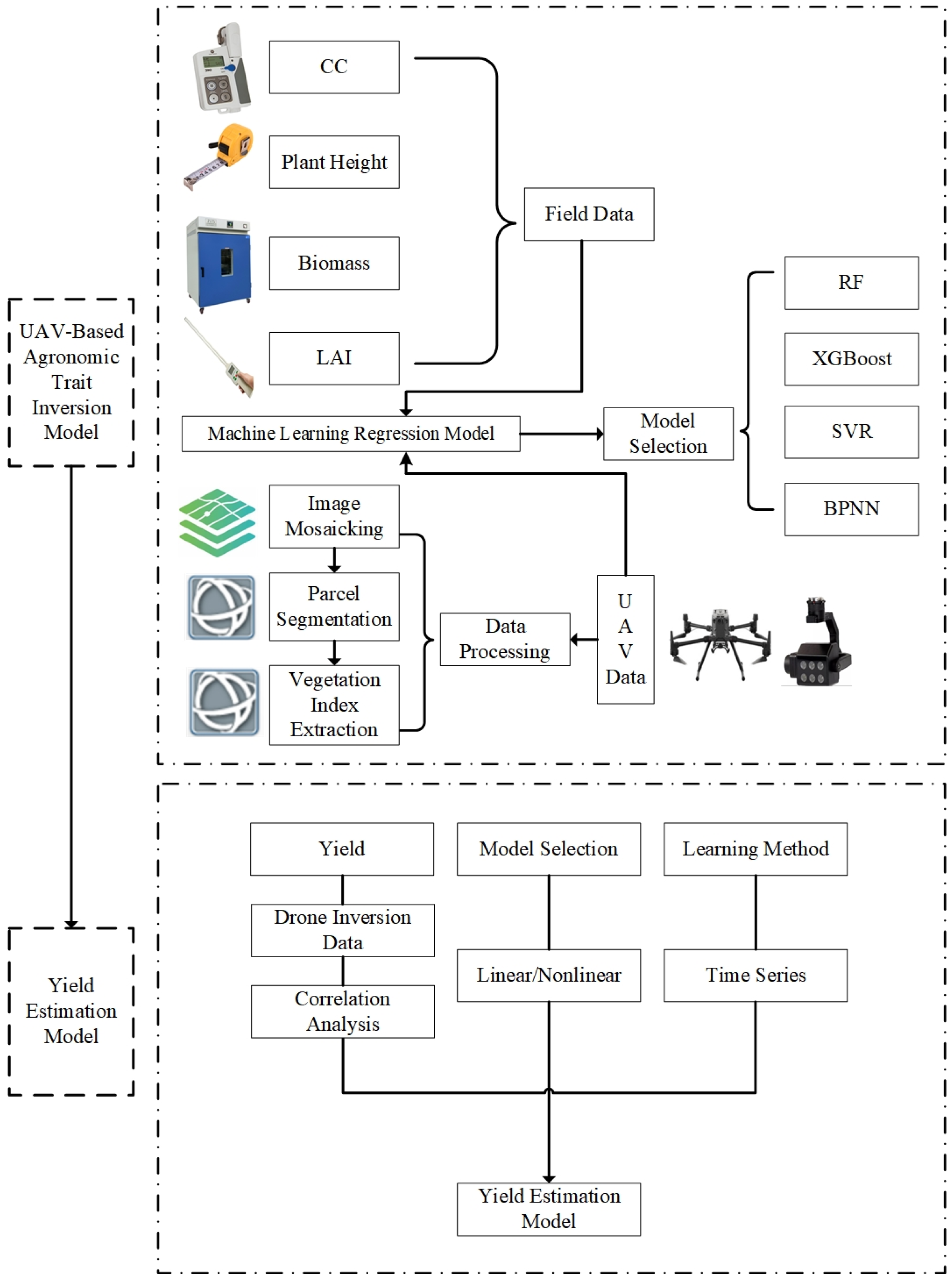
Workflow diagram of the study. The diagram illustrates the key steps of the research process: (1) collection of field data, including chlorophyll content (CC), plant height, biomass, and leaf area index (LAI); (2) acquisition and preprocessing of UAV multispectral data, involving image stitching, cropping, and extraction of vegetation indices; (3) development of inversion models (RF, XGBoost, SVR, BPNN) by correlating vegetation indices with field data, followed by selection of the most accurate model for field inversion; (4) construction of a rice yield estimation model using correlation analysis between yield and inversion data, comparing linear and nonlinear models across different phenological stages via time-series analysis.
Figure 2.
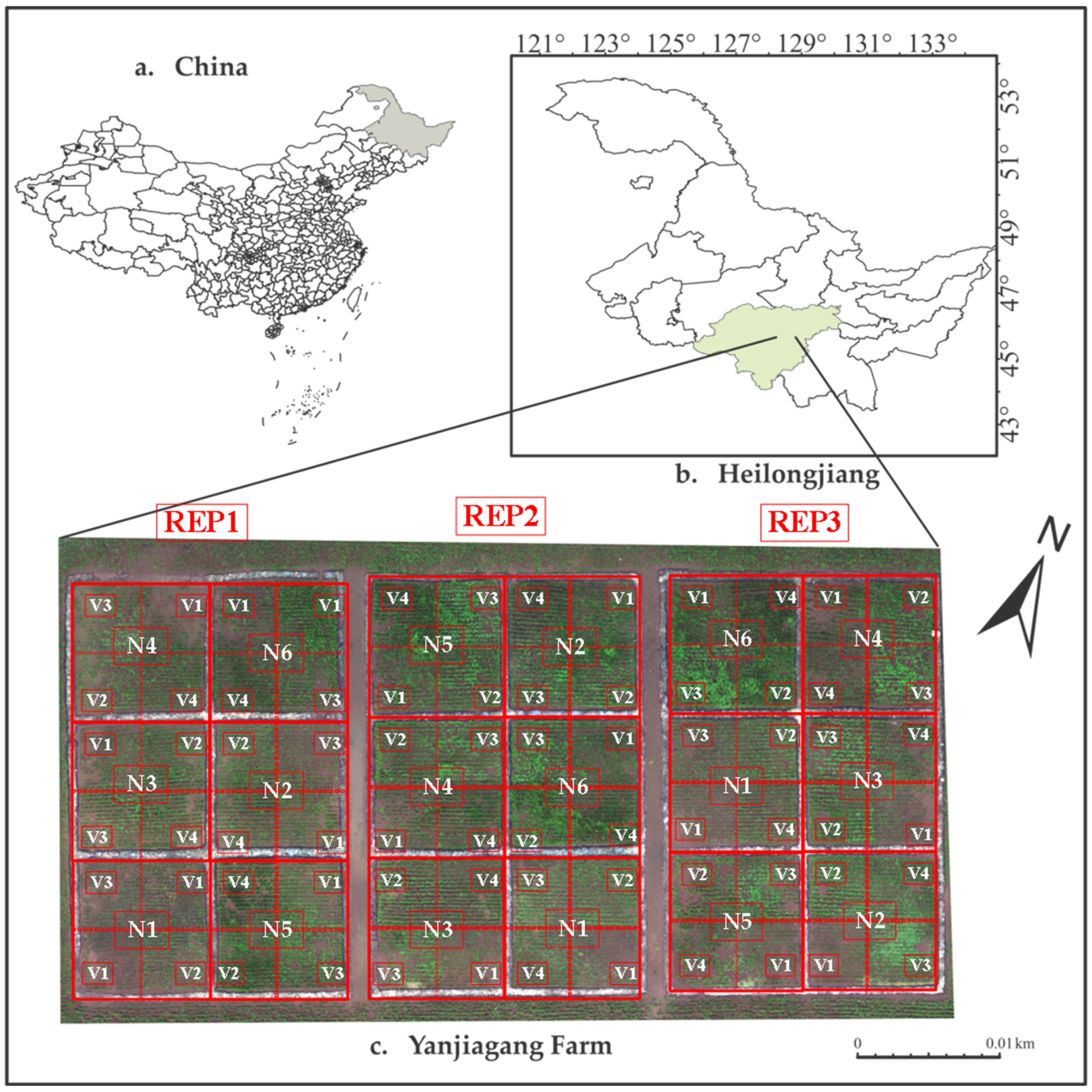
Overview of the experimental study area. The UAV image depicts the layout of the experimental plots. (a) Map of China; (b) map of Heilongjiang Province; and (c) map of Yanjiagang Farm, where V1, V2, V3, and V4 denote the four rice varieties, Kongyu131, Songjing22, Chuangyou31, and Tianlongyou619, respectively, and N1–N6 indicate different nitrogen treatments with increasing concentrations. Projection system: WGS 84.
Figure 3.
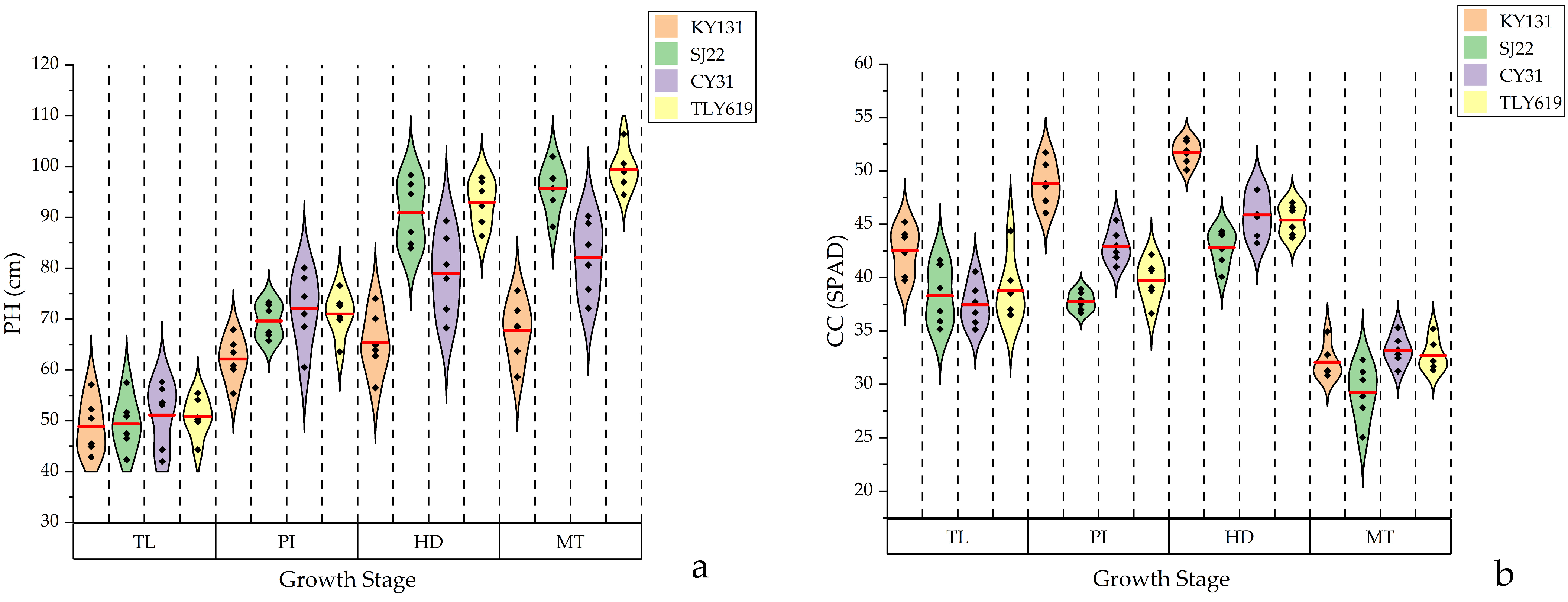
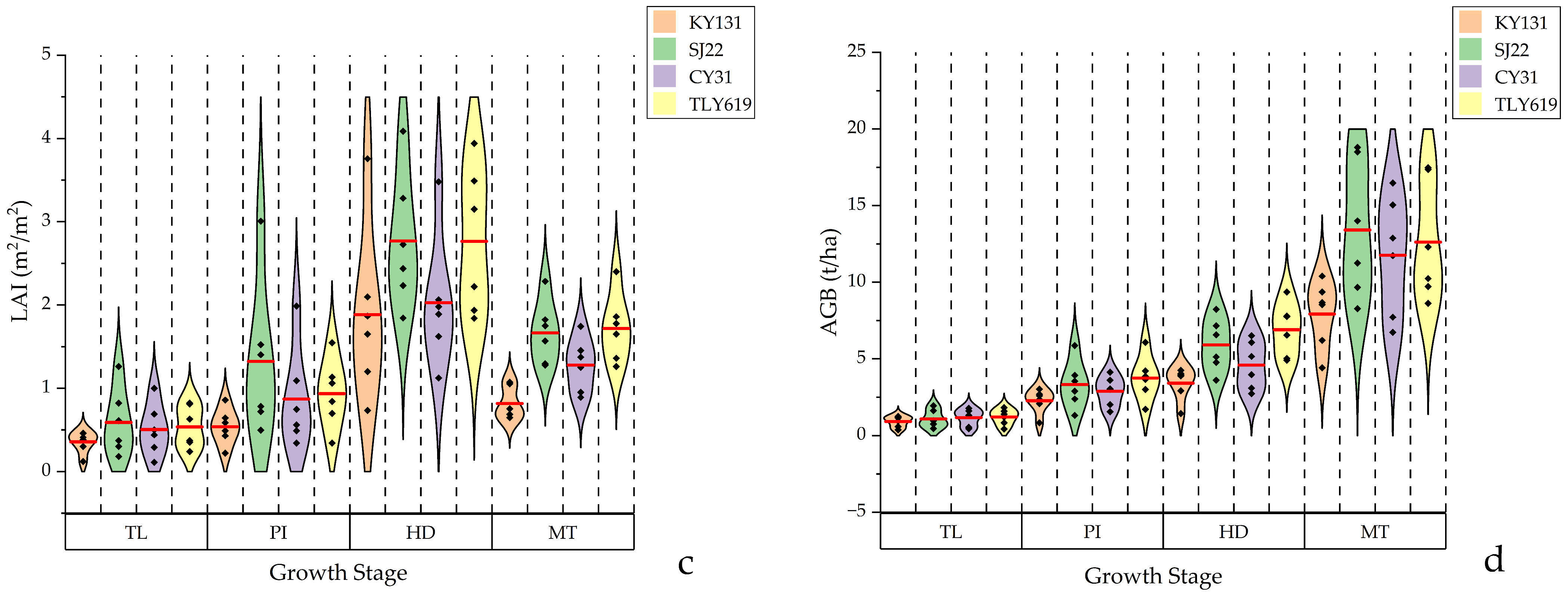
Comparison of measured phenotypic parameters among four varieties (KY131, SJ22, CY31, TLY619) at four key growth stages (TL, PI, HD, MT). (a) PH; (b) CC; (c) LAI; (d) AGB. Note: The red line in the figure represents the mean value of each variety.
Figure 3.
Comparison of measured phenotypic parameters among four varieties (KY131, SJ22, CY31, TLY619) at four key growth stages (TL, PI, HD, MT). (a) PH; (b) CC; (c) LAI; (d) AGB. Note: The red line in the figure represents the mean value of each variety.
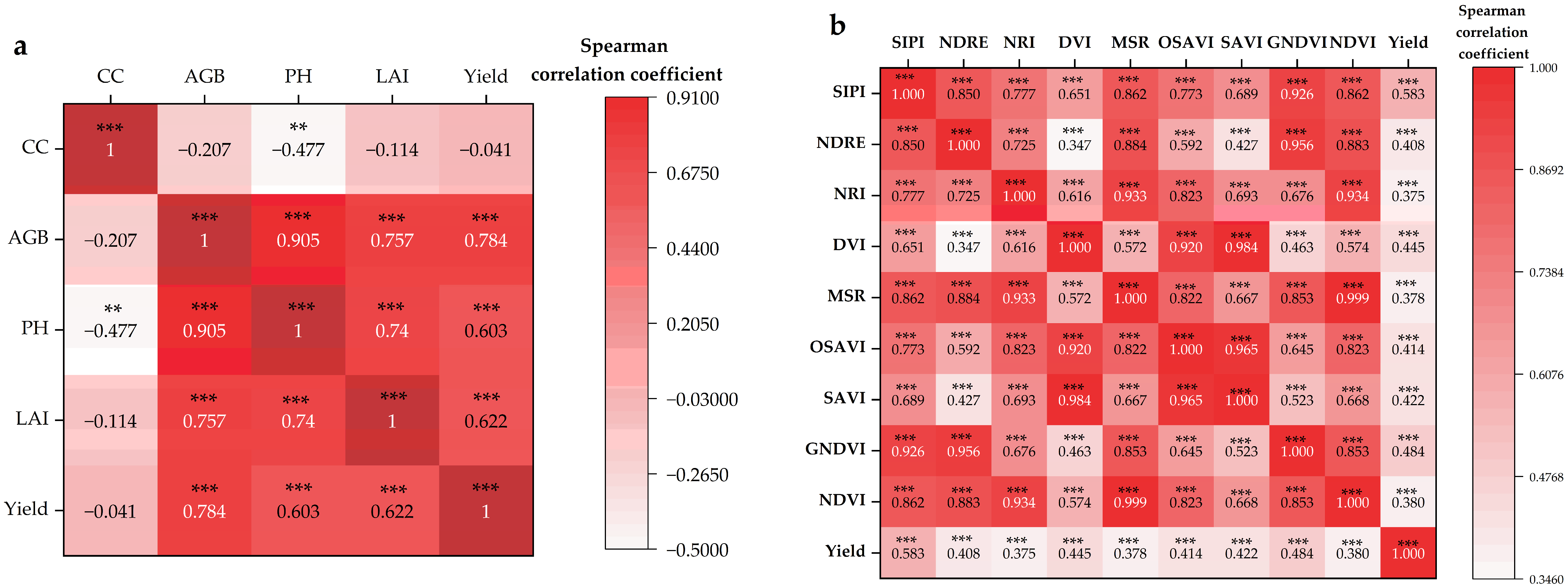
Figure 4.
Spearman correlation analysis: (a) between rice phenotypic traits and yield; (b) between vegetation indices and yield. Note: *** and ** indicate significant correlations at p < 0.01 and p < 0.05, respectively.
Figure 4.
Spearman correlation analysis: (a) between rice phenotypic traits and yield; (b) between vegetation indices and yield. Note: *** and ** indicate significant correlations at p < 0.01 and p < 0.05, respectively.
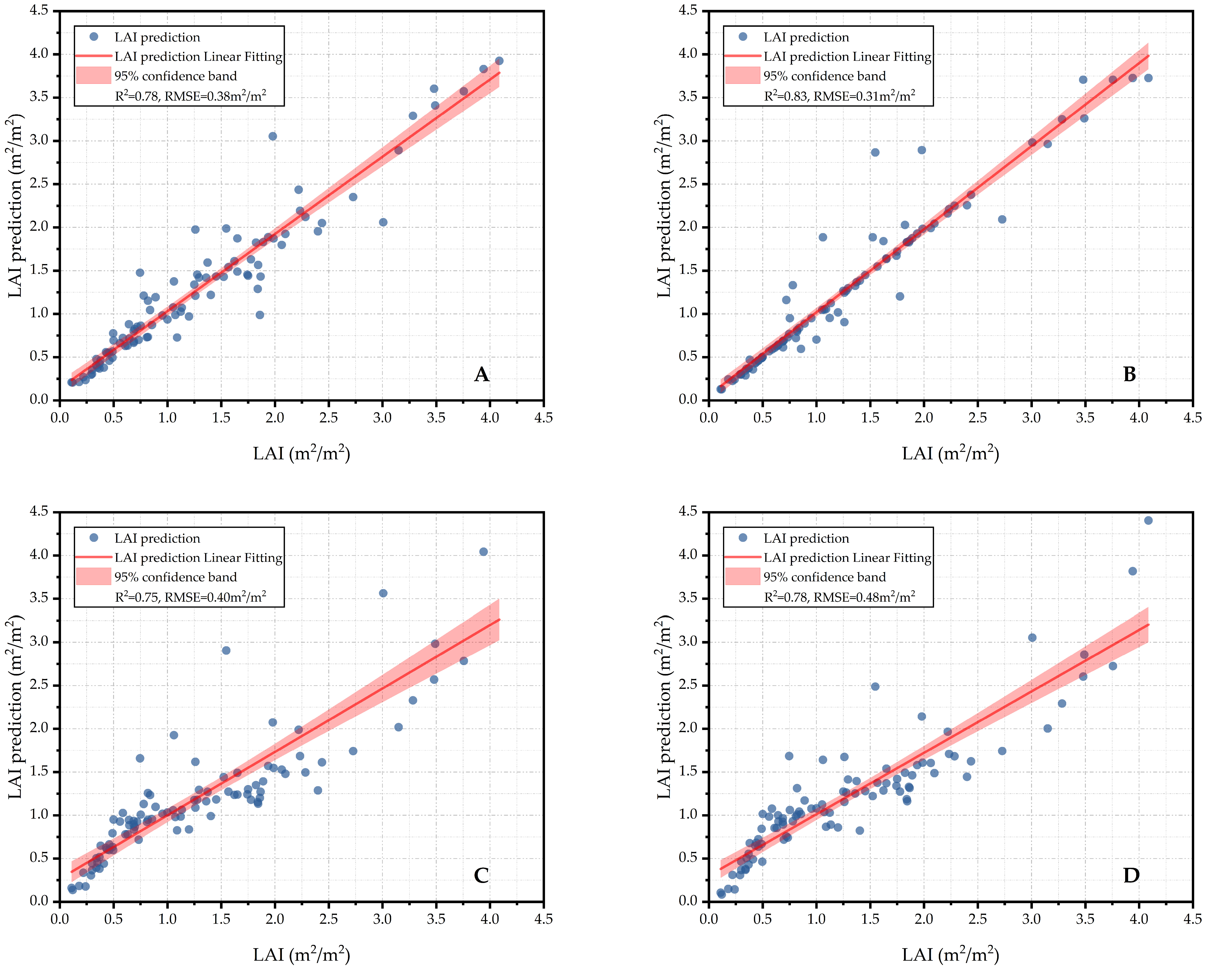
Figure 5.
Validation of UAV-derived LAI prediction models using vegetation indices. Scatter plots of ground-truth vs. predicted values: (A) RF; (B) XGBoost; (C) SVR; (D) BPNN.
Figure 5.
Validation of UAV-derived LAI prediction models using vegetation indices. Scatter plots of ground-truth vs. predicted values: (A) RF; (B) XGBoost; (C) SVR; (D) BPNN.
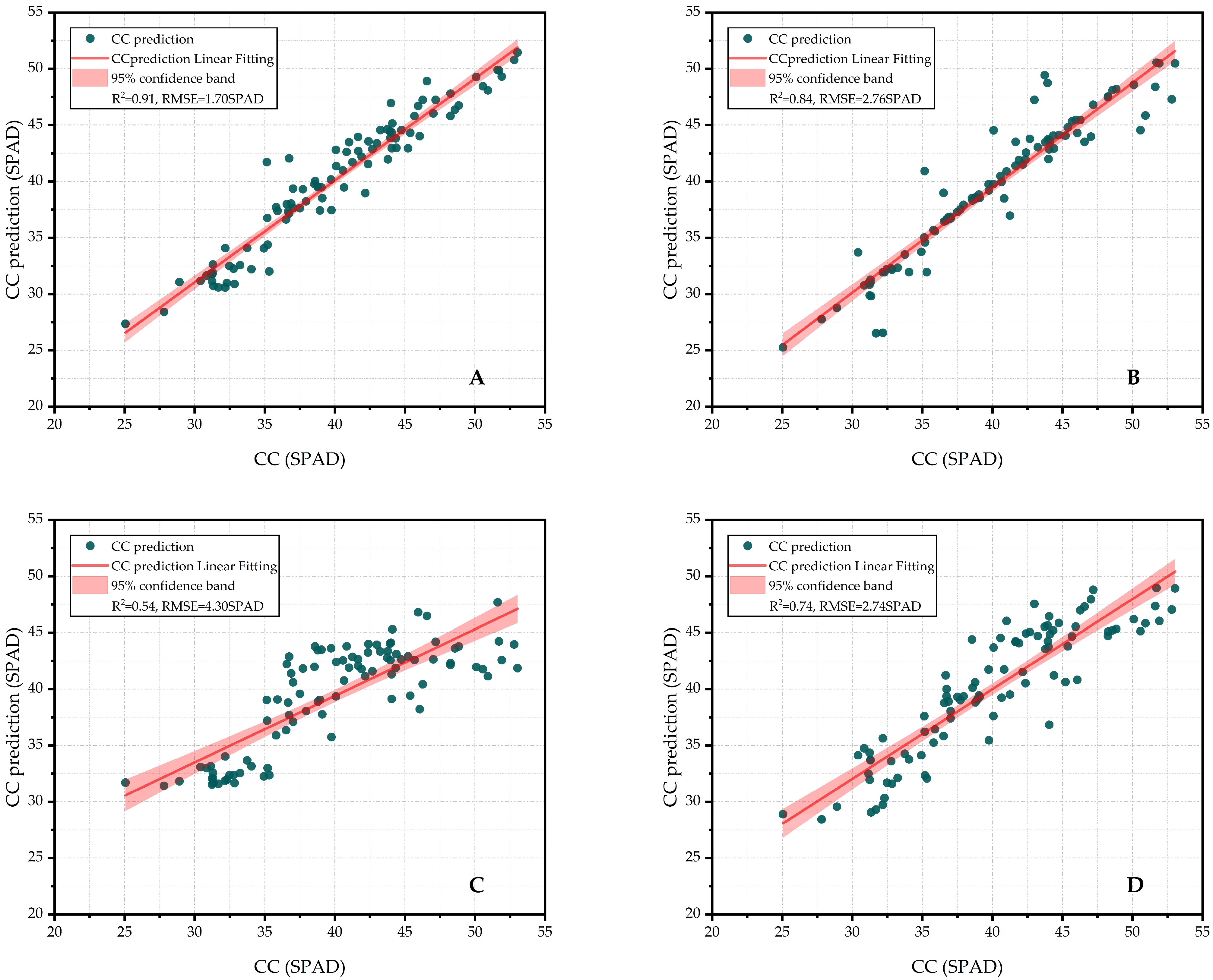
Figure 6.
Validation of UAV-derived CC prediction models using vegetation indices. Scatter plots of ground-truth vs. predicted values: (A) RF; (B) XGBoost; (C) SVR; (D) BPNN.
Figure 6.
Validation of UAV-derived CC prediction models using vegetation indices. Scatter plots of ground-truth vs. predicted values: (A) RF; (B) XGBoost; (C) SVR; (D) BPNN.
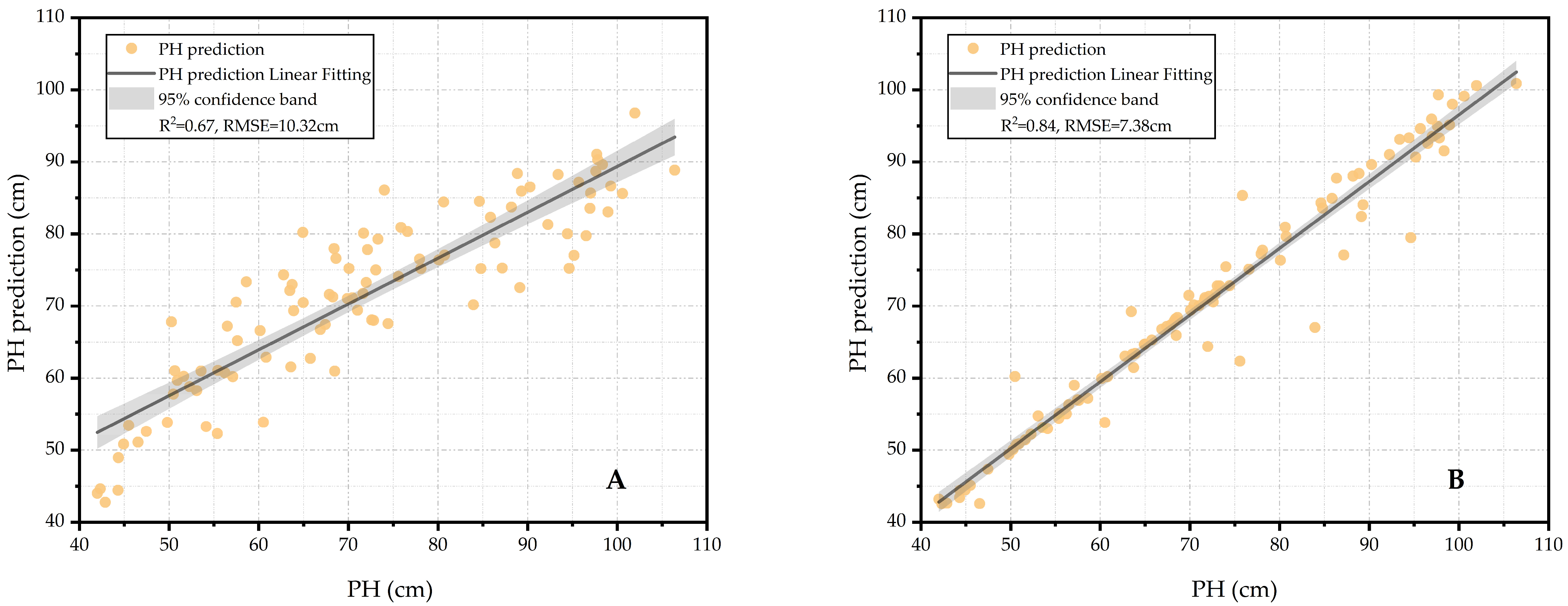
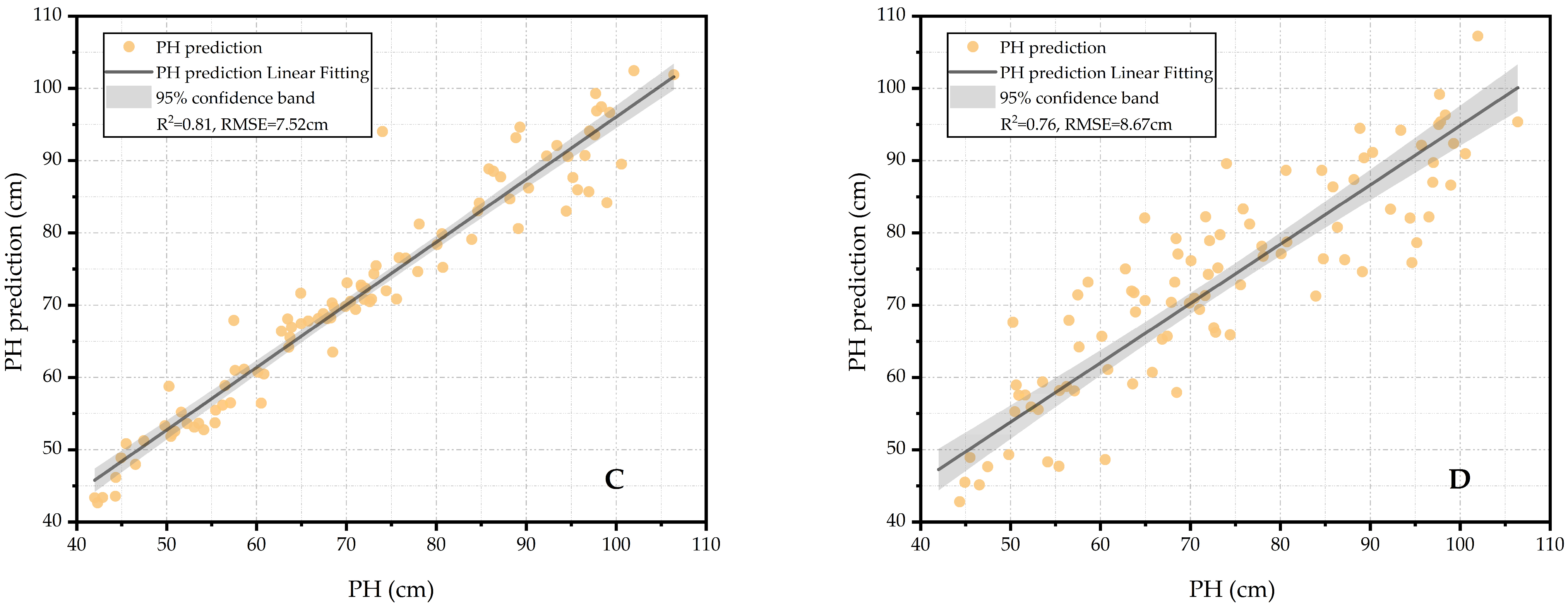
Figure 7.
Validation of UAV-derived PH prediction models using vegetation indices. Scatter plots of ground-truth vs. predicted values: (A) RF; (B) XGBoost; (C) SVR; (D) BPNN.
Figure 7.
Validation of UAV-derived PH prediction models using vegetation indices. Scatter plots of ground-truth vs. predicted values: (A) RF; (B) XGBoost; (C) SVR; (D) BPNN.
Figure 8.
Validation of UAV-derived AGB prediction models using vegetation indices: Scatter plots of ground-truth vs. predicted values: (A) RF; (B) XGBoost; (C) SVR; (D) BPNN.
Figure 8.
Validation of UAV-derived AGB prediction models using vegetation indices: Scatter plots of ground-truth vs. predicted values: (A) RF; (B) XGBoost; (C) SVR; (D) BPNN.
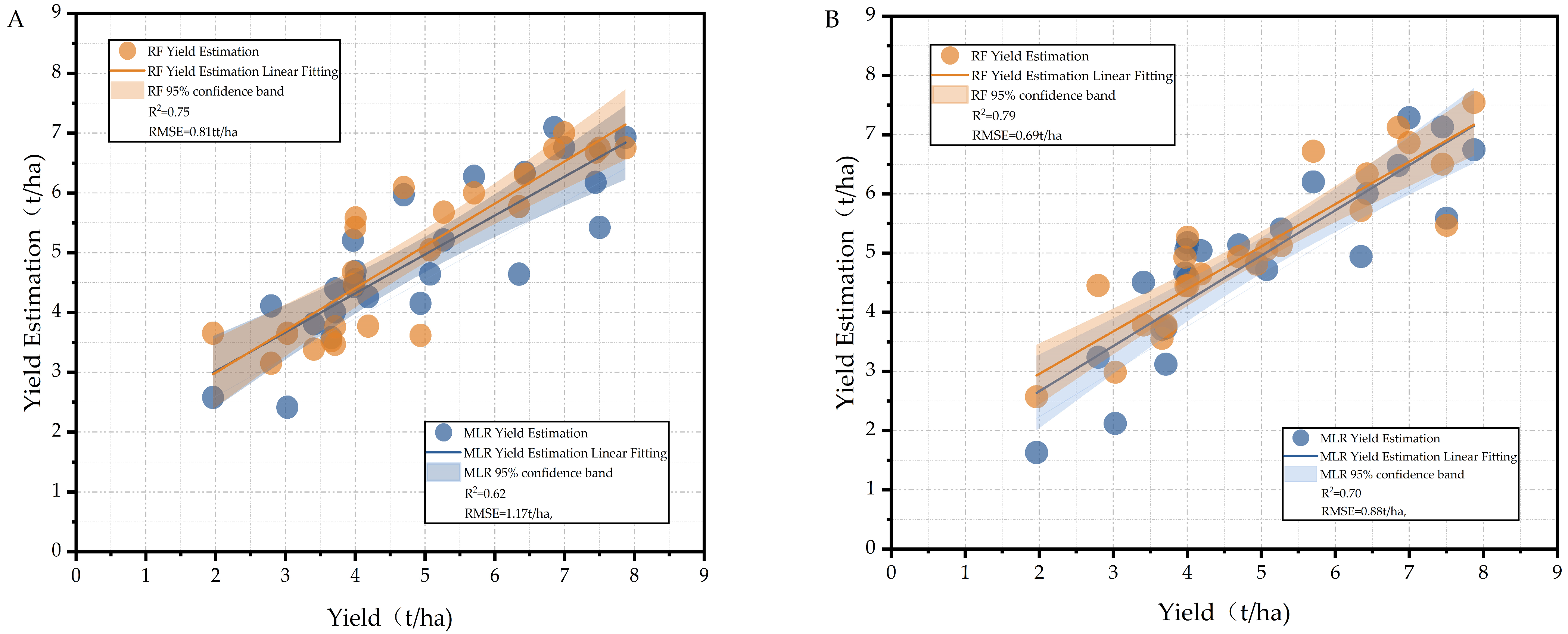
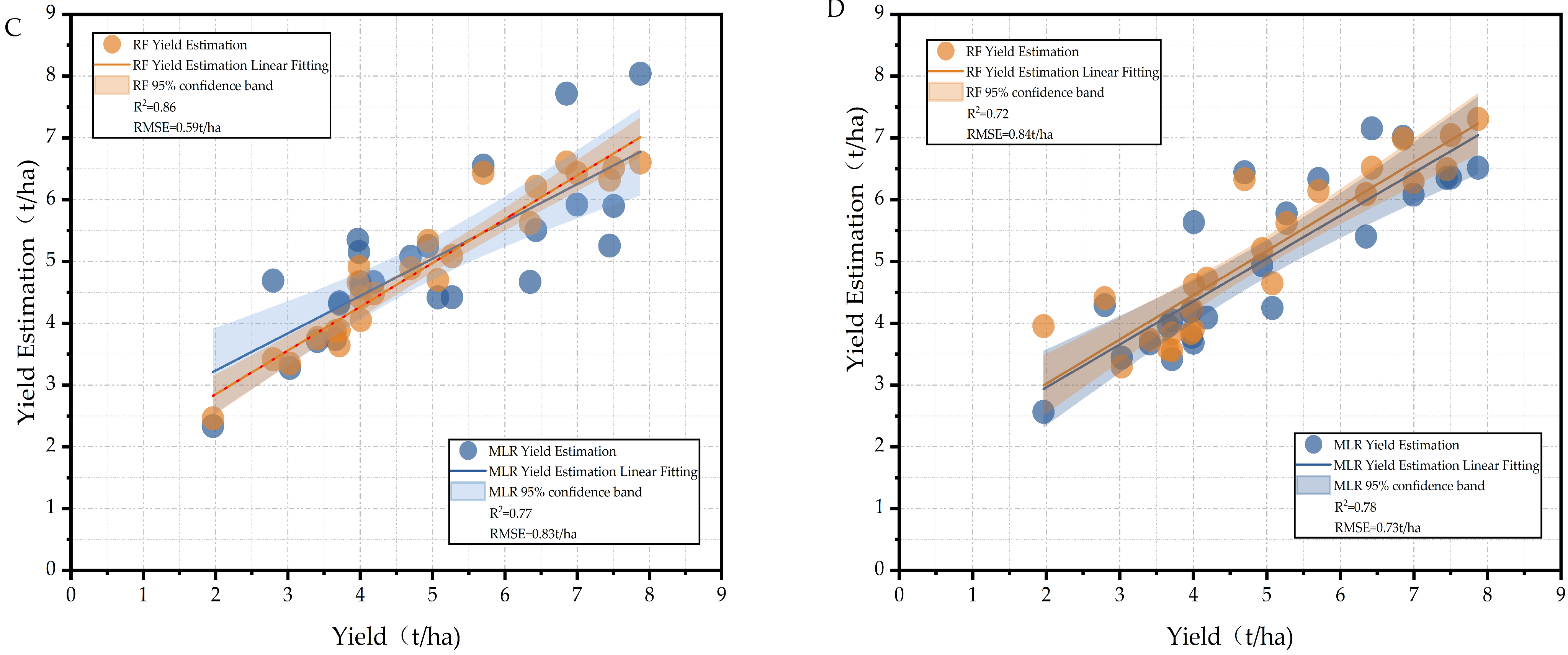
Figure 9.
Performance comparison of rice yield models across growth stages, evaluating RF and MLR algorithms with phenotypic parameters. (A) TL stage, (B) PI stage, (C) HD stage, (D) MT stage.
Figure 9.
Performance comparison of rice yield models across growth stages, evaluating RF and MLR algorithms with phenotypic parameters. (A) TL stage, (B) PI stage, (C) HD stage, (D) MT stage.
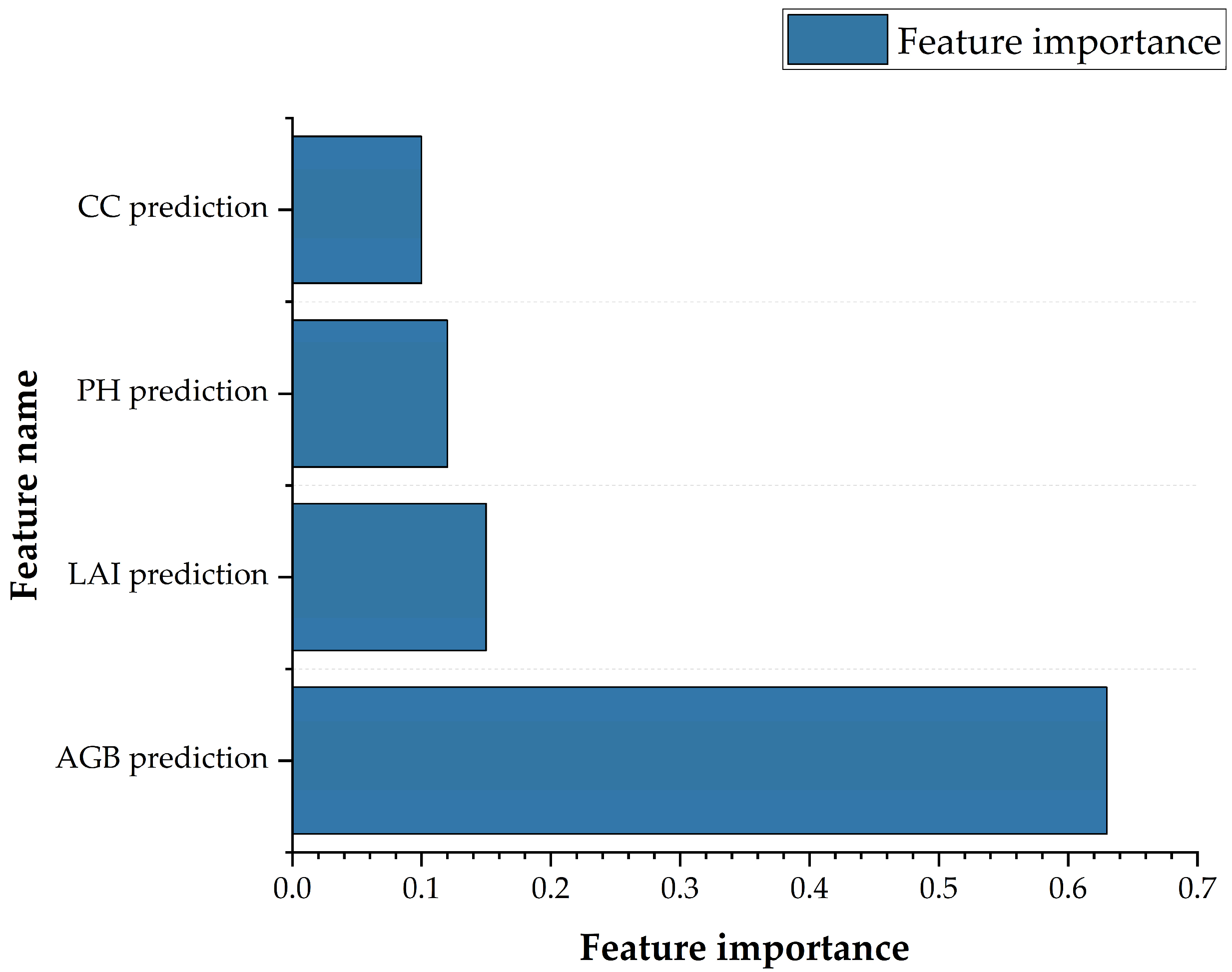
Figure 10.
Feature importance of the RF yield estimation model at the HD stage.
Figure 10.
Feature importance of the RF yield estimation model at the HD stage.
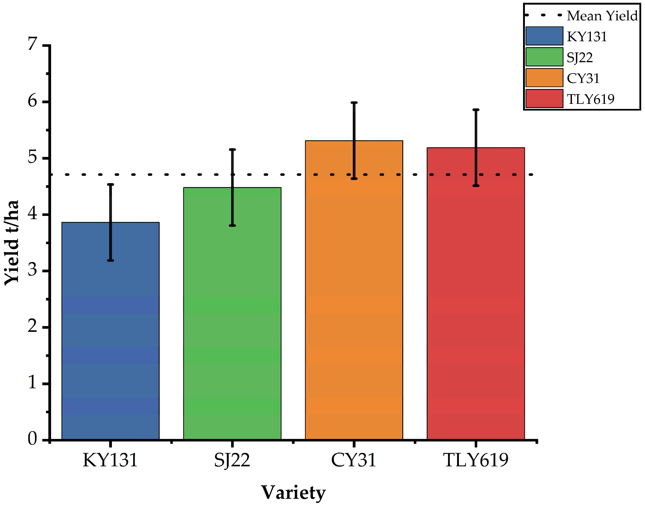
Figure 11.
Comparison of actual yield differences among varieties. Note: Yield differences were observed between conventional japonica rice varieties (KY131, SJ22) and hybrid japonica rice varieties (CY31, TLY619). The bars represent mean ± standard deviation (SD), with data based on 6 treatments and 3 field replicates.
Figure 12.
Residual plot of the yield estimation model across rice varieties. Each point represents the average yield across six treatments for the corresponding variety. The area between the dashed lines indicates the interval within which the prediction error is less than the model’s RMSE.
Figure 12.
Residual plot of the yield estimation model across rice varieties. Each point represents the average yield across six treatments for the corresponding variety. The area between the dashed lines indicates the interval within which the prediction error is less than the model’s RMSE.
Table 1.
Information on tested rice varieties used in the experiment.
Table 1.
Information on tested rice varieties used in the experiment.
| Group | Variety | Abbreviation | Variety Characteristics | Days to Maturity |
|---|
| Conventional japonica rice | Kongyu131 | KY131 | Early-maturing | 127 D |
| Songjing22 | SJ22 | Late-maturing | 144 D |
| Hybrid japonica rice | Chuangyou31 | CY31 | Early-maturing | 129 D |
| Tianlongyou619 | TLY619 | Late-maturing | 139 D |
Table 2.
Vegetation indices and their formulas.
Table 2.
Vegetation indices and their formulas.
| Vegetation Index | Formula | Reference |
|---|
| NDVI | | Rouse, J. W et al., 1974 [20] |
| GNDVI | | Anatoly A et al., 1996 [21] |
| SAVI | | A.R Huete et al., 1988 [22] |
| OSAVI | | Geneviève Rondeaux et al., 1988 [23] |
| MSR | | Compton J et al., 1979 [24] |
| DVI | | Filella, 1995 [25] |
| NRI | | Jordan et al., 1969 [26] |
| NDRE | | Barnes et al., 2000 [27] |
| SIPI | | Peñuelas et al., 1995 [28] |
Table 3.
Comparison of the RMSE and R2 obtained by RF, XG Boost, SVR, and BPNN regression models for predicting four rice phenotypic parameters: LAI, CC, PH, and AGB.
Table 3.
Comparison of the RMSE and R2 obtained by RF, XG Boost, SVR, and BPNN regression models for predicting four rice phenotypic parameters: LAI, CC, PH, and AGB.
| Model Type | | LAI | CC | PH | AGB |
|---|
| RF | RMSE | 0.38 (m2/m2) | 1.70 (SPAD) | 7.38 (cm) | 1.74 (t/ha) |
| R2 | 0.78 | 0.91 | 0.84 | 0.86 |
| XG Boost | RMSE | 0.31 (m2/m2) | 2.76 (SPAD) | 7.52 (cm) | 1.94 (t/ha) |
| R2 | 0.83 | 0.84 | 0.81 | 0.82 |
| SVR | RMSE | 0.40 (m2/m2) | 4.30 (SPAD) | 10.32 (cm) | 3.46 (t/ha) |
| R2 | 0.75 | 0.54 | 0.67 | 0.61 |
| BPNN | RMSE | 0.48 (m2/m2) | 2.74 (SPAD) | 8.67 (cm) | 1.85 (t/ha) |
| R2 | 0.78 | 0.74 | 0.76 | 0.73 |
Table 4.
Accuracy comparison of yield estimation models: predicted phenotypic parameters vs. direct vegetation indices (VIs) using RF and MLR algorithms across four growth stages: TL, PI, HD, and MT.
Table 4.
Accuracy comparison of yield estimation models: predicted phenotypic parameters vs. direct vegetation indices (VIs) using RF and MLR algorithms across four growth stages: TL, PI, HD, and MT.
| Model Type | | TL | PI | HD | MT |
|---|
| Phenotypic Parameters | VIs | Phenotypic Parameters | VIs | Phenotypic Parameters | VIs | Phenotypic Parameters | VIs |
|---|
| MLR | RMSE | 1.17 (t/ha) | 1.35 (t/ha) | 0.88 (t/ha) | 1.10 (t/ha) | 0.83 (t/ha) | 1.44 (t/ha) | 0.84 (t/ha) | 0.80 (t/ha) |
| R2 | 0.62 | 0.31 | 0.70 | 0.39 | 0.77 | 0.41 | 0.72 | 0.37 |
| RF | RMSE | 0.81 (t/ha) | 1.24 (t/ha) | 0.69 (t/ha) | 0.82 (t/ha) | 0.59 (t/ha) | 1.06 (t/ha) | 0.73 (t/ha) | 1.46 (t/ha) |
| R2 | 0.75 | 0.44 | 0.79 | 0.38 | 0.86 | 0.50 | 0.78 | 0.38 |
