A Study on Predicting Natural Gas Prices Utilizing Ensemble Model

Abstract

Natural gas, a key low-emission energy source with significant strategic value in modern energy systems, necessitates accurate forecasting of its market price to ensure effective policy planning and economic stability. This paper proposes an ensemble framework to enhance natural gas price forecasting accuracy across multiple temporal scales (weekly and monthly) by constructing hybrid models and exploring diverse ensemble strategies, while balancing model complexity and computational efficiency. For weekly data, an Autoregressive Integrated Moving Average (ARIMA) model optimized via 5-fold cross-validation captures linear patterns, while the Long Short-Term Memory (LSTM) network captures nonlinear dependencies in the residual component after seasonal and trend decomposition based on LOESS (STL). For monthly data, the superior-performing model (ARIMA or SARIMA) is integrated with LSTM to address seasonality and trend characteristics. To further improve forecasting performance, three diverse ensemble techniques including stacking, bagging, and weighted averaging are individually implemented to synthesize the predictions of the two baseline models. The bagging ensemble method slightly outperforms other models on both weekly and monthly data, achieving MAPE, MAE, RMSE, and $R^2$ values of 9.60%, 0.3865, 0.5780, and 0.8287 for the weekly data, and 11.43%, 0.5302, 0.6944, and 0.7813 for the monthly data, respectively. The accurate forecasting of natural gas prices is critical for energy market stability and the realization of sustainable development goals.

1. Introduction

As a low-emission energy source, natural gas serves as a pivotal component in global energy systems and has become a crucial choice for the energy transition in numerous countries. It is well known that the prediction of natural gas can facilitate effective policy formulation by governments, ensure secure energy supply to humans, and optimize investment returns on energy projects, thereby supporting sustainable development. However, natural gas prices are subject to significant volatility due to geopolitical tensions, supply disruptions, and fluctuating demand, posing challenges for both market participants and policymakers. From a macroeconomic perspective, persistent price increases in natural gas can trigger cost–push inflation dynamics, where rising input costs propagate through production chains and contribute to broader price-level pressures [1,2]. At the same time, the efficiency of energy markets, in which prices are expected to reflect all publicly available information, imposes inherent limits on predictability, consistent with the semi-strong form of the Efficient Market Hypothesis [3]. In recent years, the application of natural gas has expanded significantly across various sectors, including power generation, petroleum, and transportation. Driven by the global transition away from coal and the increasing adoption of natural gas as a low-emission energy source, the accurate forecasting of natural gas prices has emerged as a vital concern across energy markets, industrial operations, and policy planning [4].

Owing to the criticality of natural gas price forecasting, some work has studied how to predict commodity prices through different models. For example, Li and Kong [5] constructed the ARIMA, the SARIMA, and the ARIMA-GARCH models to predict natural gas prices. The corresponding shows that SARIMA is the best model for time series data with the seasonal effect and trend effect. Moreover, Su et al. [6] conducted predictive modeling of natural gas prices using four individual machine learning methods, and evaluated their forecasting performance separately. Bilgili and Pinar [7] employed a LSTM network to forecast gross energy consumption (GEC) in Turkey and compared its performance with the SARIMA model, with results indicating that the LSTM model generally outperforms SARIMA. For forecasting liquefied natural gas prices, Kim et al. [8] compared simple recurrent neural networks, LSTM network, and the gated recurrent unit model. The LSTM network demonstrates superior performance in modeling nonlinear and volatile time series by efficiently capturing long-term dependencies and mitigating the vanishing gradient issue.

The aforementioned works focus mainly on individual models such as ARIMA, SARIMA, and LSTM to compare their predictive performance. Nevertheless, ensemble models are capable of combining the strengths of various individual models. More recently, this issue has received much attention. He et al. [9] proposed a novel hybrid framework that integrates the SARIMA with model with a Convolutional Neural Network (CNN) and LSTM network, for high-frequency tourism demand forecasting. The model leverages SARIMA to extract linear components, CNN to capture hierarchical data structures, and LSTM to model long-term temporal dependencies. Parasyris et al. [10] evaluated the efficacy of SARIMA, LSTM, and hybrid models in forecasting meteorological variables for a two-day weather prediction in Greece, revealing that hybrid methodologies outperformed others for temperature and wind speed. Moreover, Peirano et al. [11] proposed a hybrid SARIMA-LSTM framework designed to robustly capture linear and nonlinear temporal dependencies in inflation rate forecasting for five emerging economies in Latin America, demonstrating superior predictive accuracy compared to standalone models and other combined approaches. Tahyudin et al. [12] demonstrated that the hybrid SARIMA-LSTM framework significantly enhances forecasting accuracy for US COVID-19 case predictions, with reduced RMSE and MAE compared to individual SARIMA and LSTM models. Yu and Song [13] developed a multi-stage hybrid model (VMD-GRU-AE-MLP-RF) that combines decomposition, correlation-based feature grouping, group-specific deep learning networks, and ensemble integration through random forest to enhance natural gas price forecasting performance. However, few existing studies have systematically compared the impact of different ensemble methods on forecasting performance.

However, despite the proliferation of hybrid and decomposition-based models, most adopt fixed integration mechanisms without systematic evaluation of alternative ensemble strategies. To illustrate the landscape and limitations of recent studies,

Table 1. Reference methodologies.

Reference Number	Methodologies
[14]	GA-optimized VMD-LSTM hybrid model for decomposition-based forecasting
[15]	STL-VMD-BiLSTM for enhanced wind speed forecasting
[16]	VMD-FMM-Transformer for natural gas forecasting in non-seasonal regions
[17]	Attention-based LSTM with dynamic window and GA optimization for production forecasting
[18]	SOA-optimized GRU with EEMD and sentiment analysis for crude oil price forecasting
[19]	A MSGWO optimized ELM with EEMD for natural gas price forecasting

summarizes representative works in natural gas price forecasting.

As summarized in Table 1, an increasing number of studies have adopted hybrid and data-driven approaches for natural gas price forecasting. However, several key limitations remain in the existing literature. For instance, many models rely on fixed ensemble strategies. Deep learning models such as LSTM have demonstrated strong performance but often suffer from overfitting and high computational complexity. In contrast, traditional statistical models are constrained by linear assumptions and are therefore unable to capture nonlinear dynamics inherent in time series data.

To overcome these challenges, some works have investigated various ensemble approaches to integrating individual models, such as stacking ensemble methods, bagging methods, and weighted average methods. For example, Abdellatif et al. [20] proposed a stacking ensemble learning model to forecast day-ahead PV power. In addition, Nguyen and Byeon [21] employed a stacking ensemble model utilizing logistic regression (LR) as the meta-classifier to enhance predictive performance, combined with five base learners to improve the early detection of depression in Parkinson’s disease patients. Li et al. [22] employed four machine learning models as base learners, and logistic regression was adopted as the meta-learner to construct a stacking ensemble model for predicting regional CO₂ concentrations. This hybrid model demonstrated high accuracy and reliability in the forecasting task. Duan et al. [23] improved SVR performance through the complete ensemble empirical mode decomposition with adaptive noise (CEEMDAN) preprocessing and the bagging ensemble. Moreover, Adnan et al. [24] integrated the Locally Weighted Learning (LWL) algorithm with the bagging ensemble technique to forecast streamflow in the Jhelum Basin, Pakistan, while Wang et al. [25] presented an ensemble model which combines three individual models using a weighted approach to forecast natural gas prices. Shashvat et al. [26] introduced a weighted averaging framework for forecasting infectious disease incidence rates, such as typhoid fever, and evaluated its performance against conventional predictive models through comparative analysis.

To facilitate a more intuitive comparison of ensemble methods,

Table 2. Reference ensemble methods.

Reference Number	Ensemble Methods
[27]	CEEMD with PSO-SVM and MS-GARCH for final prediction
[28]	Stacking ensemble with Lasso regression for short-term load forecasting
[29]	EEMD-EELM decomposition-ensemble for crude oil price forecasting
[30]	Improved stacking with walk-forward validation for carbon price forecasting

summarizes recent studies with respect to different integration approaches.

As shown in Table 2, ensemble learning is increasingly applied in forecasting methods. However, most studies have focused on a single integration strategy and lack a unified comparative evaluation.

To better assess the contribution of forecasting models to sustainability, this study reviews and compares the temporal scale choices adopted by previous researchers in energy forecasting, with a systematic summary provided in

Table 3. Reference time scale.

Reference Number	Time Scale
[31]	Daily
[32]	Weekly
[33]	Daily
[34]	Monthly
[35]	Daily
[36]	Monthly
[13]	Split the monthly data into daily data

.

As illustrated in Table 3, most existing research is confined to a single time scale or split high-frequency data into a lower temporal resolution, with limited systematic assessment of forecasting performance across temporal resolutions. However, this paper addresses this gap through a comparative analysis on two time scales such as weekly and monthly natural gas price predictions.

Based on the aforementioned studies, it is evident that relying solely on a single model, a single integration approach, or considering only one time scale may entail certain limitations. To address these limitations, this paper investigates natural gas price forecasting accuracy across two distinct time scales by constructing multiple hybrid models and exploring various ensemble strategies. Firstly, the model is constructed using two distinct temporal scales such as weekly and monthly data. The natural gas price series are decomposed via the STL method into interpretable trend, seasonal trend, and residual trend. Considering the trade-off between model complexity and predictive accuracy, for the weekly data, a 5-fold cross-validation procedure is applied to fit an ARIMA model to capture linear patterns in the time series, while an LSTM network is employed to model temporal dependencies and uncover potential nonlinear dynamics within the residual component. For the monthly data, 5-fold cross-validation is similarly used to fit both ARIMA and SARIMA models to the linear component, and their forecasting performance results are compared based on error metrics; the superior model is selected for subsequent ensemble integration. Concurrently, the LSTM network is applied to extract nonlinear features from the residual series. Finally, to explore the optimal strategy for enhancing predictive performance, this study conducts a comprehensive comparison of three ensemble methods: stacking, bagging, and weighted averaging. The primary objective is to identify the most effective integration approach under different temporal scales, thereby optimizing the synergy between the statistical (ARIMA or SARIMA) and deep learning (LSTM) components.

The subsequent sections are arranged as follows. In Section 2, some definitions of the ARIMA, SARIMA model, and LSTM network are given, and the evaluation metrics for forecasting performance are introduced briefly. Section 3 illustrates three ensemble methods such as stacked ensemble, bagging ensemble, and weighted average ensemble and describes the construction of ARIMA, SARIMA, and LSTM models, as well as their ensemble counterparts, at two temporal scales for natural gas price forecasting. Finally, a short discussion and conclusion is given in Section 4.

2. Methodology

This section provides an overview of the ARIMA, SARIMA model, and LSTM network. Then, we shall present different evaluation indicators in order to assess the predictive accuracy of models.

2.1. ARIMA

Stationarity is a fundamental assumption in time series, which serves as a prerequisite for statistical inference and parameter estimation. The ARMA model is typically used for modeling and forecasting when the data are stationary. For $ARMA(p,q)$, we have

$$y_t={\varphi }_0+{\varphi }_1{y}_{t-1}+\cdots +{\varphi }_p{y}_{t-p}+{\epsilon }_t-{\theta }_1{\epsilon }_{t-1}-\cdots -{\theta }_q{\epsilon }_{t-q},$$

(1)

where $y_t$ denotes the response variable at time $t\in T$, ${\varphi }_0$ represents the intercept term, the autoregressive parameters ${\varphi }_i(i=1,2,\cdots ,p)$ quantify the linear dependence between the current observation and its preceding p lagged observations, ${\epsilon }_t$ is the white noise, and ${\theta }_j(j=1,2,\cdots ,q)$ stands for the moving average parameters that can reflect the impact of past errors on the current observation. Furthermore, Model (1) can be expressed as

$${\varphi }_p\left(L\right)x_t={\Theta }_q\left(L\right){\epsilon }_t,$$

where the p-order autoregressive coefficient polynomial ${\Phi }_p\left(L\right)=1-{\sum }_{i=1}^p{\varphi }_i{L}^i$, the q-order moving average coefficient polynomial ${\Theta }_q\left(L\right)=1-{\sum }_{i=1}^q{\theta }_i{L}^i$, and L represents the lag operator.

Box and Jenkins [37] proposed the ARIMA model which is a widely recognized statistical forecasting technique that addresses non-stationarity in time series data by applying d-order differencing to achieve stationarity prior to parameter estimation. The ARIMA model is given by

$${\varphi }_p\left(L\right){\Delta }^d{x}_t={\Theta }_q\left(L\right){\epsilon }_t,$$

(2)

where the differentiating operator ${\nabla }^d={(1-L)}^d$. Thus, we denote model (2) as $ARIMA(p,d,q)$.

2.2. SARIMA

In practice, time series often exhibit significant seasonal trends, and the SARIMA model is commonly employed to solve these problems. The $SARIMA(p,d,q)\times {(P,D,Q)}_s$ model takes the form of

$${\varphi }_p\left(L\right)A_P\left(L^s\right){\Delta }^d{\Delta }_s^D{y}_t={\Theta }_q\left(L\right)B_Q\left(L^s\right){\epsilon }_t,$$

(3)

where $A_P\left(L^s\right)=1-{\sum }_{i=1}^P{A}_i{L}^{s,i}$ is the seasonal polynomial $AR\left(P\right)$, $A_i$ denotes the seasonal autoregressive coefficient corresponding to lag i, $B_Q\left(L^s\right)=1-{\sum }_{i=1}^Q{B}_i{L}^{s,i}$ is the seasonal polynomial $MA\left(Q\right)$, $B_i$ represents the seasonal moving average parameter at lag i, and s defines the seasonal period. The operator for seasonal differencing ${\nabla }_s^D={\left(1-L^s\right)}^D$ eliminates the seasonal non-stationarity. The modeling procedure follows a systematic approach, outlined as follows:

Step 1: Determine the optimal $SARIMA(p,d,q)\times {(P,D,Q)}_s$ configuration by analyzing the time series’ statistical properties, such as trend components and seasonal fluctuations.

Step 2: Estimating the unknown model parameters such as $p,d,q,P,D$, and Q using maximum likelihood estimation (MLE).

Step 3: Conduct diagnostic checks on the residuals to assess model adequacy, including tests for autocorrelation and overall goodness of fit.

Step 4: Produce predictive forecasts for subsequent time periods through the application of the estimated model and the utilization of existing historical data.

Based on the aforementioned theoretical analysis, it is evident that the ARIMA and SARIMA models exhibit distinct advantages in handling linear and highly seasonal time series data.

2.3. LSTM

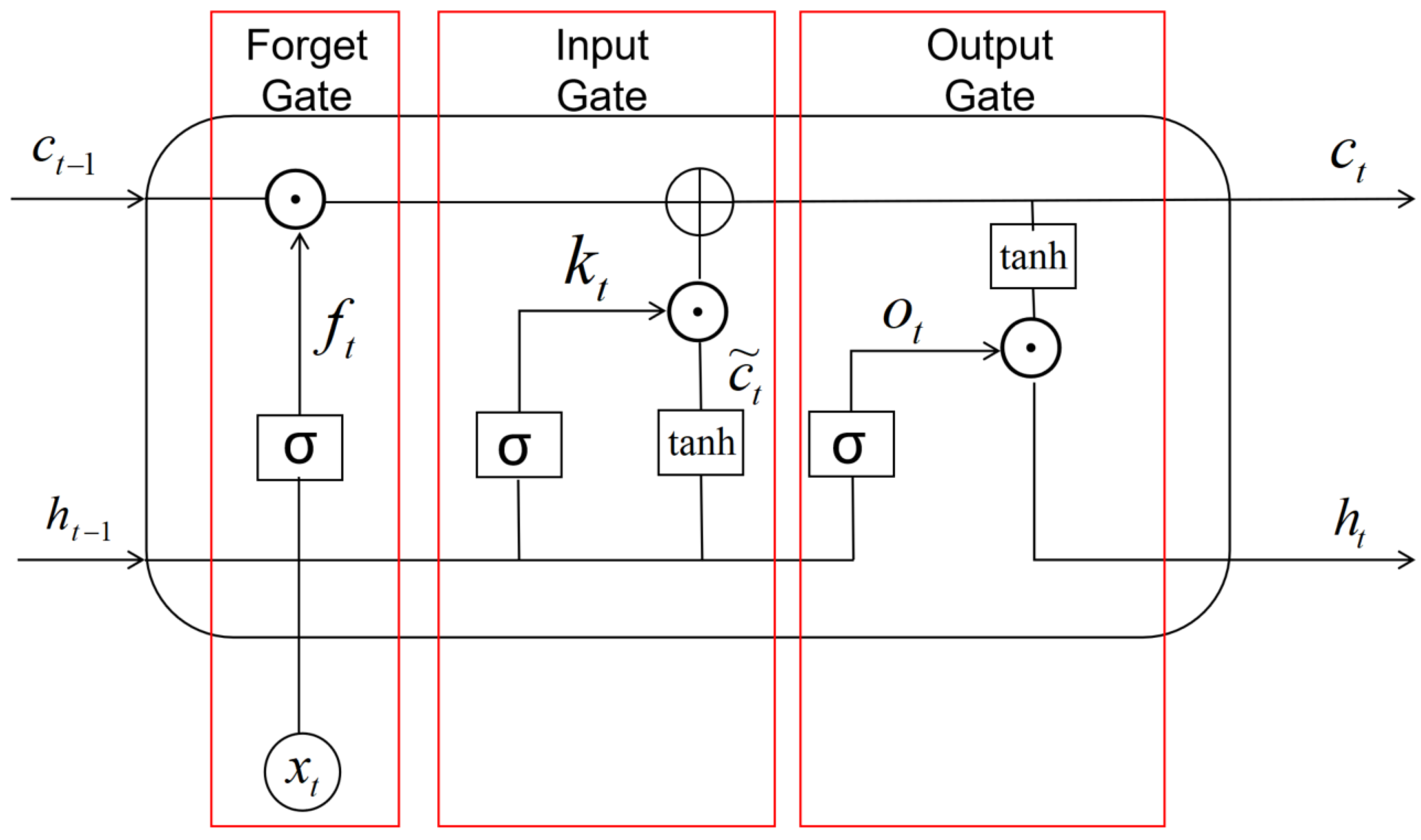
The LSTM proposed by Hochreiter and Schmidhuber [38] can overcome the recurrent neural network (RNN) shortcoming of the vanishing gradient. According to Qiu [39], the operations of the LSTM network at time t are formulated as follows.

Step 1: The forget gate activation $f_t$ is computed to filter out irrelevant information from the previous cell state,

$$f_t=\sigma \left(W_f{x}_t+U_f{h}_{t-1}+b_f\right),$$

(4)

where $\sigma$ denotes the Logistic sigmoid function, which maps its input to a value within the interval from 0 to 1, $b_f$ represents the bias term associated with the forget gate, and the weight matrices $W_f$ and $U_f$ correspond to the parameters that link the current input $x_t$ at time step t and the previous hidden state $h_{t-1}$ at time step $t-1$ to the forget gate activation $f_t$, respectively.

Step 2: The input gate determines which components of the input vector $x_t\in {\mathbb{R}}^M$ are retained in the cell state $c_t$, based on the transformed input $k_t$ generated through the gate’s activation function given by

$$k_t=\sigma \left(W_k{x}_t+U_k{h}_{t-1}+b_k\right),$$

(5)

where $b_k$ denotes the bias parameter associated with the input gate, and the weight matrices $W_k$ and $U_k$ are responsible for mapping the current input $x_t$ and the prior hidden state $h_{t-1}$ to the activation of the input gate, respectively. The candidate cell state ${\tilde{c}}_t$ can be updated by

$${\tilde{c}}_t=tanh\left(W_c{x}_t+U_c{h}_{t-1}+b_c\right),$$

(6)

where tanh represents the activation function that normalizes the input within the interval from −1 to 1, $b_c$ is the bias term for the candidate cell state, the weight matrices $W_c$ and $U_c$ connect the input $x_t$ and the previous hidden state $h_{t-1}$, contributing to the computation of the candidate cell state, respectively.

Step 3: The update of the cell state $c_t$ involves the fusion of the candidate memory ${\tilde{c}}_t$ and the previous memory $c_{t-1}$, and is formulated as

$$c_t=f_t\odot c_{t-1}+k_t\odot {\tilde{c}}_t,$$

where the symbol ⊙ stands for element-wise multiplication, and ⊕ is the sum of the elements of the vector.

Step 4: The hidden state $h_t$ is computed in the output gate by combining the output activation $o_t$, and the updated cell state $c_t$ is given

$$h_t=o_t\odot tanh\left(c_t\right)$$

with

$$o_t=\sigma \left(W_o{x}_t+U_o{h}_{t-1}+b_o\right),$$

(7)

where $b_o$ is the bias term for the output gate, and $W_o$ and $U_o$ are the weight matrices that map the current input $x_t$ and the previous hidden state $h_{t-1}$ to the output gate output, respectively.

Thus, model (4)–(7) can be succinctly described as follows:

$$\left[\begin{array}{c}{\tilde{c}}_t\\ o_t\\ k_t\\ f_t\end{array}\right]=\left[\begin{array}{c}tanh\\ \sigma \\ \sigma \\ \sigma \end{array}\right]\left(W\left[\begin{array}{c}{x}_t\\ h_{t-1}\end{array}\right]+b\right).$$

This intricate design enables the LSTM network to establish longer-distance temporal dependencies, thereby enhancing its capacity to handle time series data effectively. Furthermore, as illustrated in Figure 1, the recurrent unit structure of LSTM network mainly consists of the forget gate $f_t$, the input gate $k_t$, and the output gate $o_t$. The memory cell state, as a core element of the LSTM architecture, persists across the entire sequence and enables the controlled updating and forgetting of information through the three gating mechanisms.

2.4. Model Evaluation Metrics

To assess the predictive performance of the ensemble SARIMA-LSTM model, four widely adopted error metrics are employed, such as Mean Absolute Error (MAE), Root Mean Square Error (RMSE), Mean Absolute Percentage Error (MAPE) and the coefficient of determination ($R^2$). The MAE quantifies the average absolute deviation between predictions and observations, that is

$$\mathrm{MAE}={\displaystyle \frac{1}{n}}\sum _{t=1}^n|y_t-{\widehat{y}}_t|,$$

where n denotes the total number of observations, and ${\widehat{y}}_t$ refers to the predictions.

The RMSE represents the standard deviation of the residuals, indicating the dispersion of prediction errors relative to the true values is given by

$$\mathrm{RMSE}=\sqrt{{\displaystyle \frac{1}{n}}\sum _{t=1}^n{(y_t-{\widehat{y}}_t)}^2}.$$

Meanwhile, MAPE evaluates forecasting performance by representing prediction errors as a percentage. The MAPE is defined below:

$$\mathrm{MAPE}={\displaystyle \frac{100\%}{n}}\sum _{t=1}^n\left|{\displaystyle \frac{y_t-{\widehat{y}}_t}{y_t}}\right|.$$

Among the three evaluation metrics mentioned above, lower values signify superior model performance. $R^2$ quantifies the percentage of variability in $y_t$ accounted for by the model predictions, and is expressed as

$$R^2=1-{\displaystyle \frac{{\sum }_{t=1}^n{\left(y_t-{\widehat{y}}_t\right)}^2}{{\sum }_{t=1}^n{\left(y_t-\overline{y}\right)}^2}},$$

where $\overline{y}$ denotes the average of the observed data points. $R^2$ takes values between 0 and 1, with larger values suggesting a stronger alignment between the model predictions and the actual data.

3. Ensemble Model Construction at Two Temporal Scales

In this section, actual data are utilized to construct and evaluate ARIMA, SARIMA, and LSTM models, as well as their ensemble counterparts, at two temporal scales such as weekly and monthly for natural gas price forecasting. The primary objective is to compare their predictive performance and identify the most accurate modeling approach.

3.1. Data Source and Description

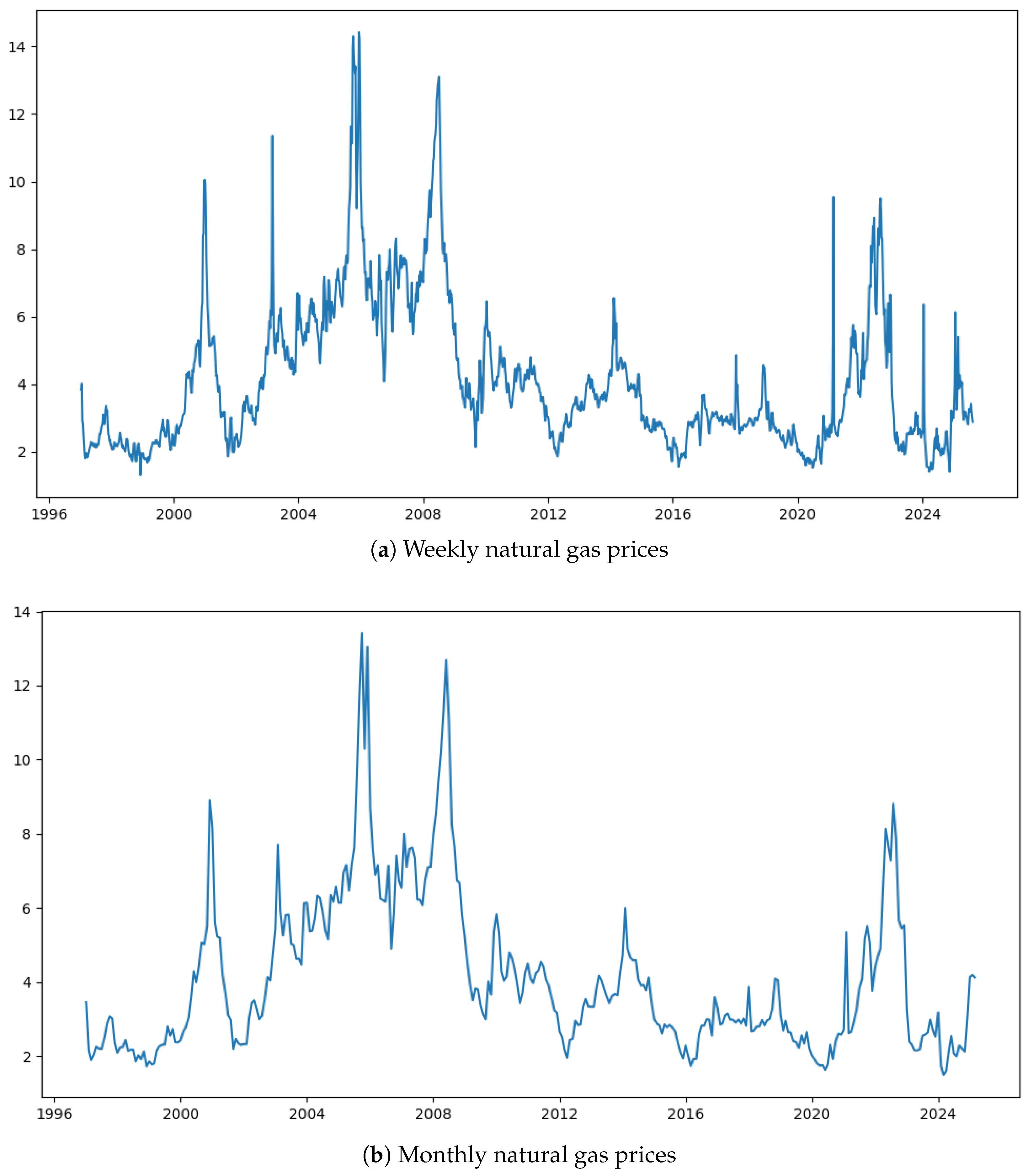
The key benchmarks for global natural gas prices that influence price fluctuations include the Henry Hub in the U.S., the Title Transfer Facility (TTF) of the Netherlands, the National Balancing Point (NBP) from the UK, the Japan Canada Cross (JCC) in Japan, and the Shanghai Energy Exchange (SHEL) in China. Due to the lack of natural gas price observations during weekends and the increased modeling complexity associated with high-frequency daily data, both weekly and monthly natural gas price data from January 1997 to August 2025 were obtained from the Henry Hub trading point (source: https://www.eia.gov/dnav/ng/hist/rngwhhdM.htm (accessed on 10 August 2025) [40]). The monthly dataset comprises $n=339$ observations, while the weekly dataset contains n = 1492 observations over the same period. Descriptive statistics for the original price series at both temporal scales are provided in

Table 4. Summary statistics of the original natural gas price data at weekly and monthly temporal scales.

	Min	${\mathit{Q}}_1$	Median	${\mathit{Q}}_3$	Max	Mean	Std
Weekly Price	1.31	2.58	3.39	5.14	14.41	4.11	2.16
Monthly Price	1.49	2.58	3.45	5.24	13.42	4.12	2.14

.

As shown in Table 4, both weekly and monthly price series show similar central tendencies, with median prices of 3.39 and 3.45 $/MMBtu, respectively. The monthly data range from 1.49 to 13.42 $/MMBtu, with a mean of 4.12 $/MMBtu and standard deviation of 2.14 $/MMBtu. The weekly data exhibit a broader range (1.31–14.41 $/MMBtu) and slightly higher variability (std = 2.16 $/MMBtu), reflecting greater short-term price fluctuations.

To observe both the temporal evolution and fundamental characteristics of the raw data at multiple scales, Figure 2 presents the time series of natural gas prices at weekly and monthly frequencies from January 1997 to August 2025.

As illustrated in Figure 2, the price series exhibits significant volatility and cyclical behavior across both time scales. The weekly data reveal more frequent fluctuations and finer short-term dynamics, including sharp spikes during periods such as 2005 and 2022, reflecting immediate market responses to supply–demand imbalances or geopolitical events. In contrast, the monthly series smooths high-frequency noise, highlighting broader trends such as the peak during 2008, the decline in the early 2010s, and the resurgence starting in 2021. Both series confirm the presence of non-stationarity and structural changes, underscoring the need for appropriate preprocessing in modeling.

To prevent information leakage and mitigate potential bias from single train–test partitioning, this study employs a 5-fold cross-validation methodology. The natural gas price series spanning January 1997 to August 2025 is divided into five consecutive, non-overlapping temporal folds. The cross-validation procedure strictly follows chronological order, with each test fold positioned temporally after its corresponding training folds. As the fold number increases, the training set progressively expands in a rolling-window manner while maintaining temporal integrity. The test sets remain non-overlapping and require no retrospective adjustments, ensuring strict adherence to the fundamental principle of temporal causality, where future observations never influence past model training. This approach provides a robust evaluation framework that captures model performance across evolving market dynamics while preserving the temporal structure of the time series data.

3.2. Modeling and Forecasting with ARIMA and SARIMA

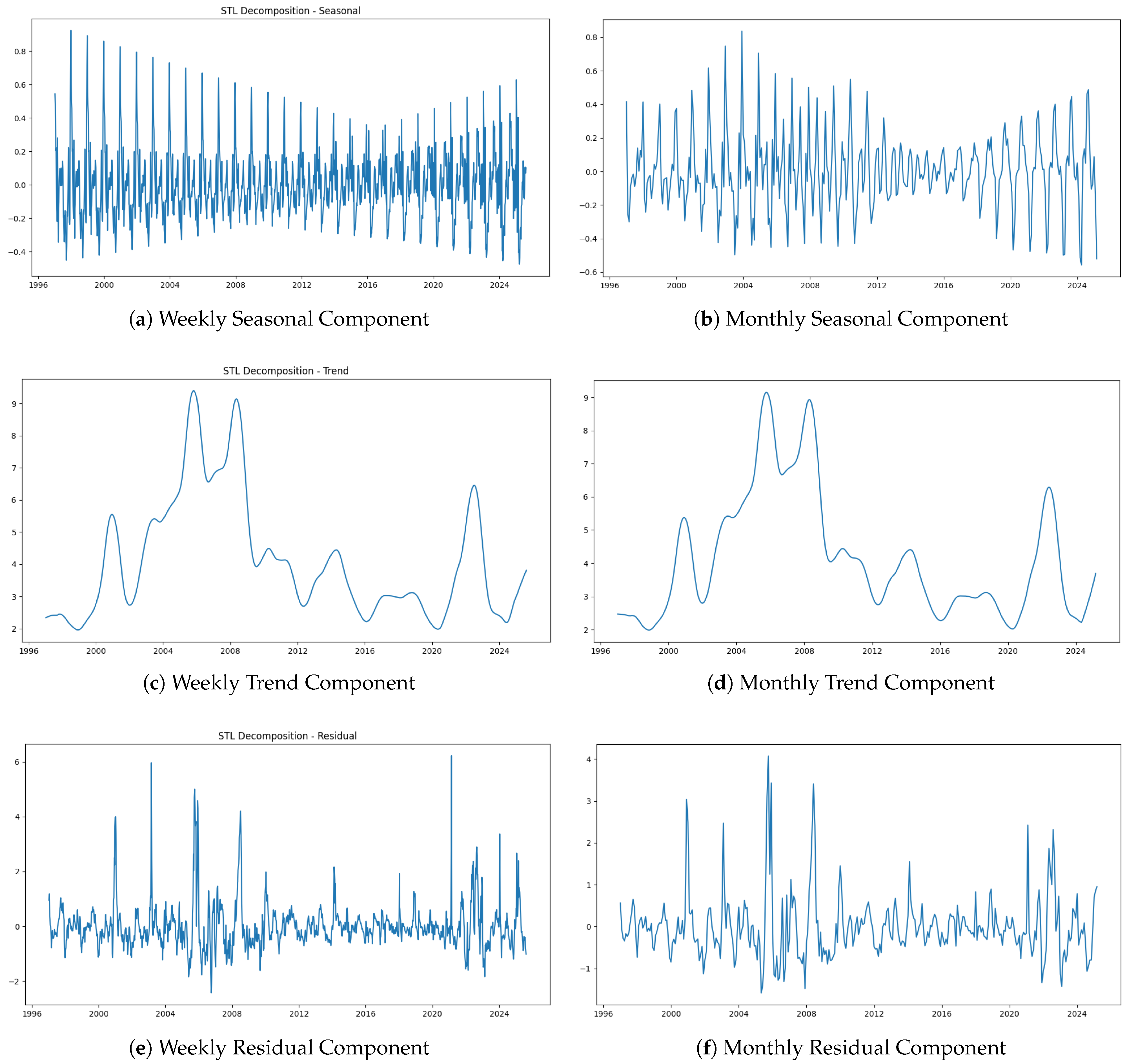
STL [41] represents a decomposition of the time series method designed to separate data into seasonal, trend, and residual components. Initially, the STL method is utilized to break down the dataset into its constituent components, followed by the visualization of their corresponding time series plots as displayed in Figure 3.

As shown in Figure 3, both weekly and monthly decompositions reveal distinct seasonal patterns: weekly seasonal components (Figure 4a) exhibit recurring fluctuations at shorter intervals, while monthly seasonal components (Figure 4b) display annual periodicity with peaks in specific months. The trend components (Figure 4c,d) show upward trajectories with volatility, confirming non-stationarity in both timeframes.

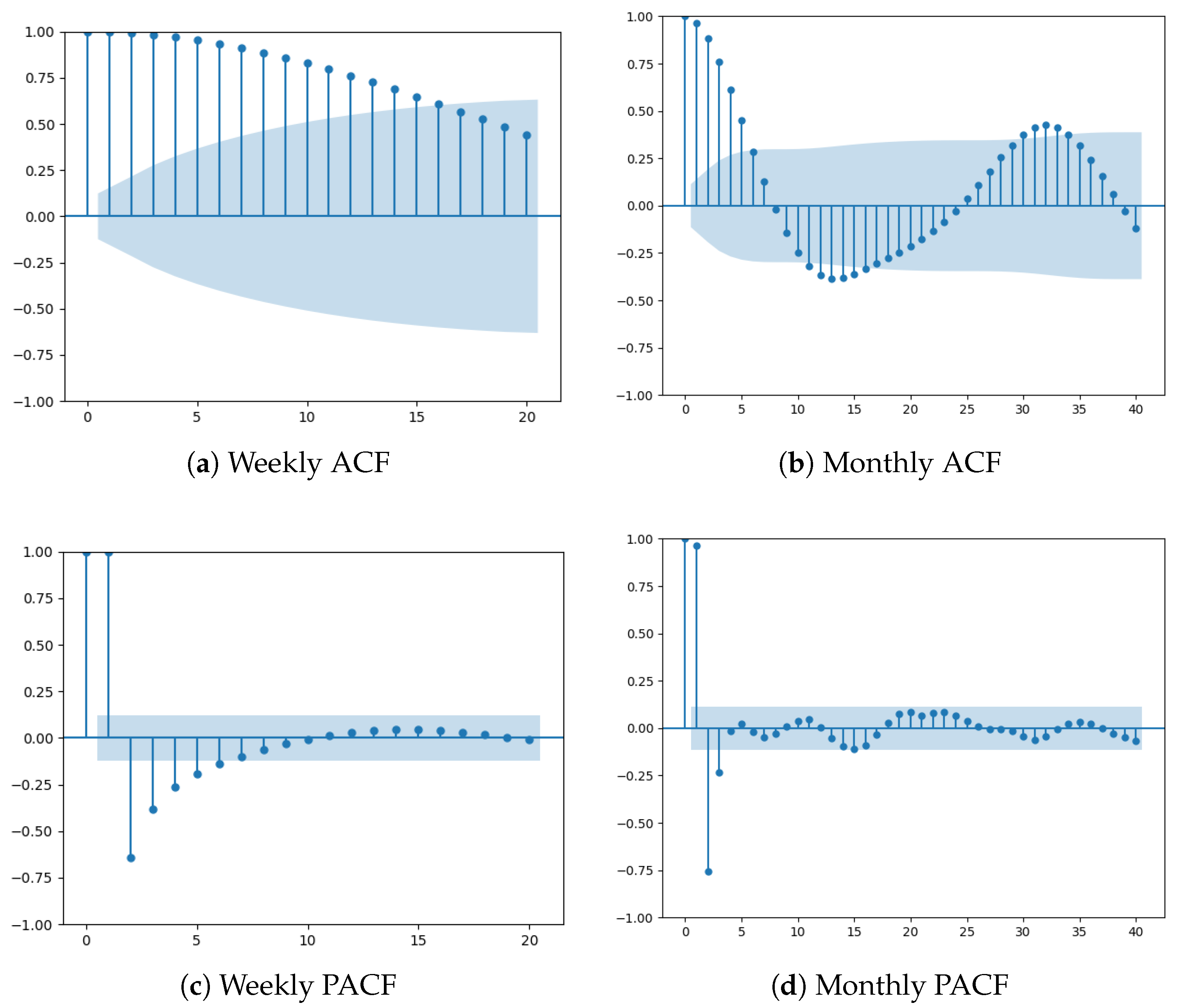
The inherent non-stationarity in the original trend component is mitigated through first-order differencing, which enhances the model’s ability to discern latent price drivers and elevates forecasting accuracy. This finding is corroborated by Augmented Dickey–Fuller (ADF) test results: the differenced weekly series exhibits an ADF statistic of −5.2354 (p = 0.008), while the monthly series yields a test statistic of −3.789 (p = 0.003). Both outcomes demonstrate statistical significance at conventional thresholds, confirming the stationarity of the transformed time series across temporal resolutions. Additionally, Figure 4 displays the autocorrelation function (ACF) and partial autocorrelation function (PACF) plots for the two temporal scales of natural gas price series.

As illustrated in Figure 4, the ACF in Figure 4a,b reveals a gradual decline in correlations across lag terms, with notably high autocorrelation coefficients in the initial lags. Meanwhile, the PACF in Figure 4c,d demonstrates significant spikes at the first and second lags, followed by a rapid decay to near-zero values. These characteristics collectively suggest that the differenced series is primarily influenced by short-term dynamics, making it suitable for ARIMA and SARIMA modeling. Given that the dataset comprises monthly observations and exhibits clear annual seasonality, the seasonal period s is set to 12 to align with the observed 12-month periodicity.

The Akaike Information Criterion (AIC) is widely recognized in academic research as an effective method for model comparison based on information entropy, quantified through Kullback–Leibler divergence. From this perspective, considering the complexity of model construction and the computational cost, we employ five-fold cross-validation to separately construct ARIMA models for weekly data and both ARIMA and SARIMA models for monthly data, determining the optimal model based on AIC values computed across different parameter configurations. It is worth noting that in model selection based on the AIC, it is computed from a single model fit on the training window only and is not averaged across cross-validation folds. Model performance is subsequently evaluated out-of-sample using standard forecasting accuracy metrics. For the monthly data, both ARIMA and SARIMA models are fitted under identical conditions, including the same data window, parameter search grid, and computational environment. The SARIMA model with parameters $SARIMA(3,1,2)\times {(0,1,0)}_{12}$ is selected based on superior out-of-sample forecast accuracy. For the weekly data, the $ARIMA(3,1,3)$ model is chosen as the preferred model after comparative evaluation of forecasting error metrics. Based on the above analysis, the mathematical expression of the model is presented below:

$$(1-{\varphi }_{1}L-{\varphi }_2{L}^2-{\varphi }_3{L}^3){(1-L)}^1{(1-L^{12})}^1{y}_t=(1+{\theta }_{1}L+{\theta }_2{L}^2){\epsilon }_t.$$

Meanwhile, it is important to note here that STL performs separate fitting on each training window of the five-fold cross-validation for each group, and the components used for the test window are derived without peeking. The final predicted values are obtained by adding the trend component predicted by the ARIMA or SARIMA model to the corresponding seasonal component defined as

$${\widehat{y}}_t^{\mathrm{final}}={\widehat{T}}_t^{\mathrm{ARIMA}\mathrm{or}\mathrm{SARIMA}}+S_t,$$

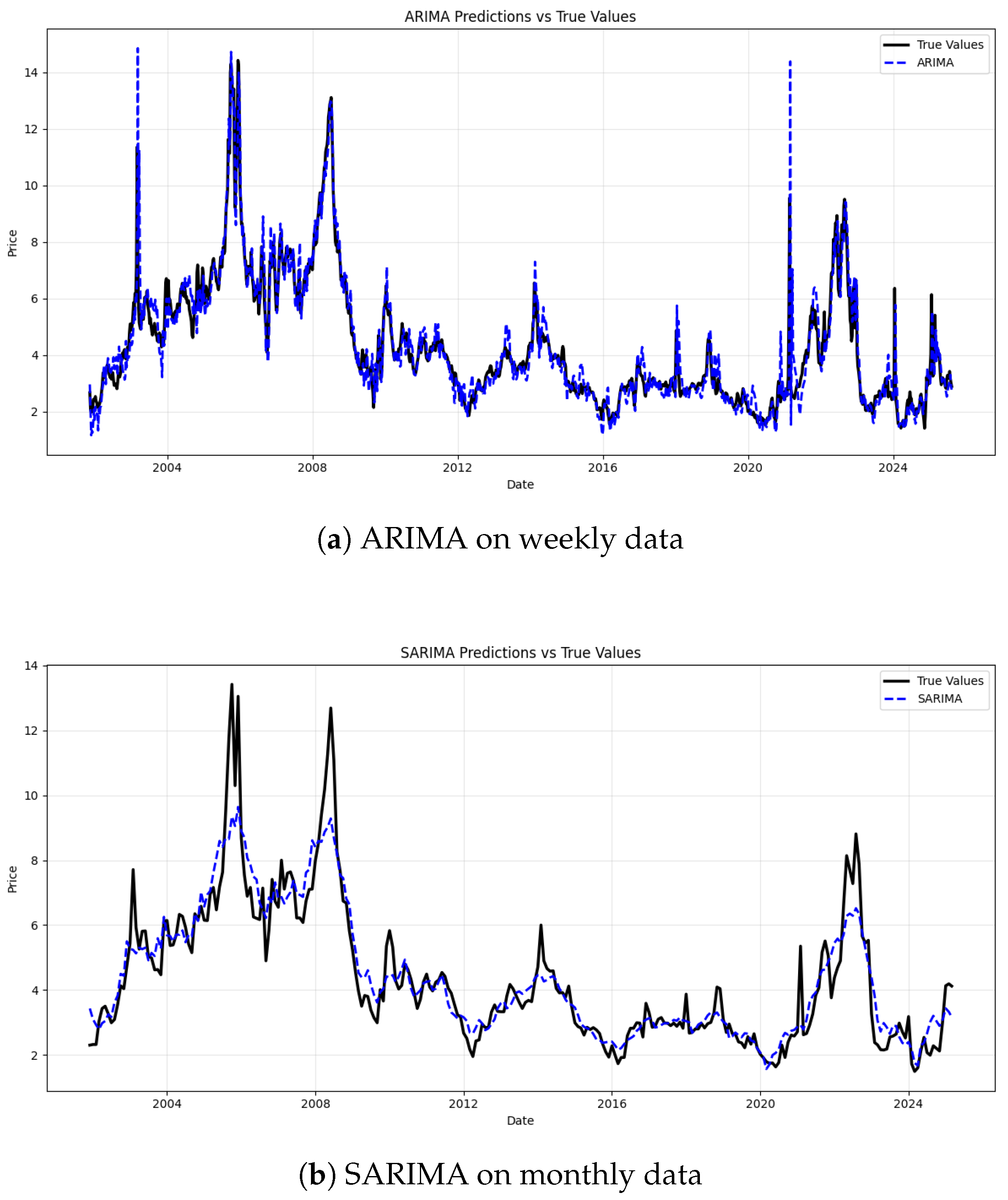
where ${\widehat{T}}_t^{\mathrm{ARIMA}\mathrm{or}\mathrm{SARIMA}}$ and $S_t$ denote the trend and seasonal components fitted by STL on the training window of each group, respectively. Meanwhile, the subsequent analysis presents separate plots of predicted versus actual values for the ARIMA model applied to weekly data and the SARIMA model applied to monthly data as illustrated in Figure 5.

As shown in Figure 5, the outcomes indicate a strong alignment between the model’s predictions and the observed data. Meanwhile, the model residuals are subjected to the Ljung–Box test post-forecasting to assess whether they conform to white noise. For the weekly and monthly data, the resulting p values are 0.2386 and 0.3345, respectively. These results indicate that the residual series are statistically consistent with white noise, supporting the validity of the model’s variance assumptions and confirming the appropriateness of ARIMA and SARIMA modeling for the given time series.

3.3. Modeling and Forecasting with LSTM

Since the LSTM model demonstrates superior performance in handling nonlinear components, an LSTM model is constructed for the residual component obtained from the STL decomposition. In order to enhance model convergence and ensure consistent variable scaling, min–max normalization is utilized in this work as follows:

$$x^{\prime }={\displaystyle \frac{x-x_{\min }}{x_{\max }-x_{\min }}},$$

where $x^{\prime }$ and x denote the original and normalized values, respectively, and $x_{\max }$ and $x_{\min }$ correspond to the maximum and minimum of the original data. It is important to emphasize here that the method is not used globally but is only computed in the training window of each fold and then applied to the test window by transformation. Additionally, the Adam optimizer is employed to minimize the MSE loss function. An early stopping mechanism is implemented during training to prevent overfitting by halting the process when the validation loss shows no improvement for a predefined number of epochs. Meanwhile, the final forecasts are generated by aggregating the trend, seasonal, and residual components predicted by the LSTM model

$${\widehat{y}}_t^{\mathrm{final}}={\mathrm{T}}_t+{\mathrm{S}}_t+{\widehat{ϵ}}_t^{\mathrm{LSTM}},$$

where ${\mathrm{S}}_t$ refers to the seasonal variation at time t which is fitted by STL on the training window of each group, and ${\widehat{ϵ}}_t^{\mathrm{LSTM}}$ denotes the residual term predicted by the LSTM model at time t. The use of a decomposition strategy allows the model to separately analyze and reconstruct both the underlying trend and transient fluctuations in the data. By employing five-fold cross-validation and grid search to identify optimal hyperparameters, the parameter configuration table for the LSTM model developed on weekly data and monthly data is presented in

Table 5. Parameter setting of LSTM model on two temporal scales.

Hyperparameters	Weekly Data	Monthly Data
Input variable count	1	1
Output variable count	1	1
Neurons count	32	50
Learning rate	0.001	0.001
Optimizer	Adam	Adam
Loss function	MSE	MSE
Training period	50	100

.

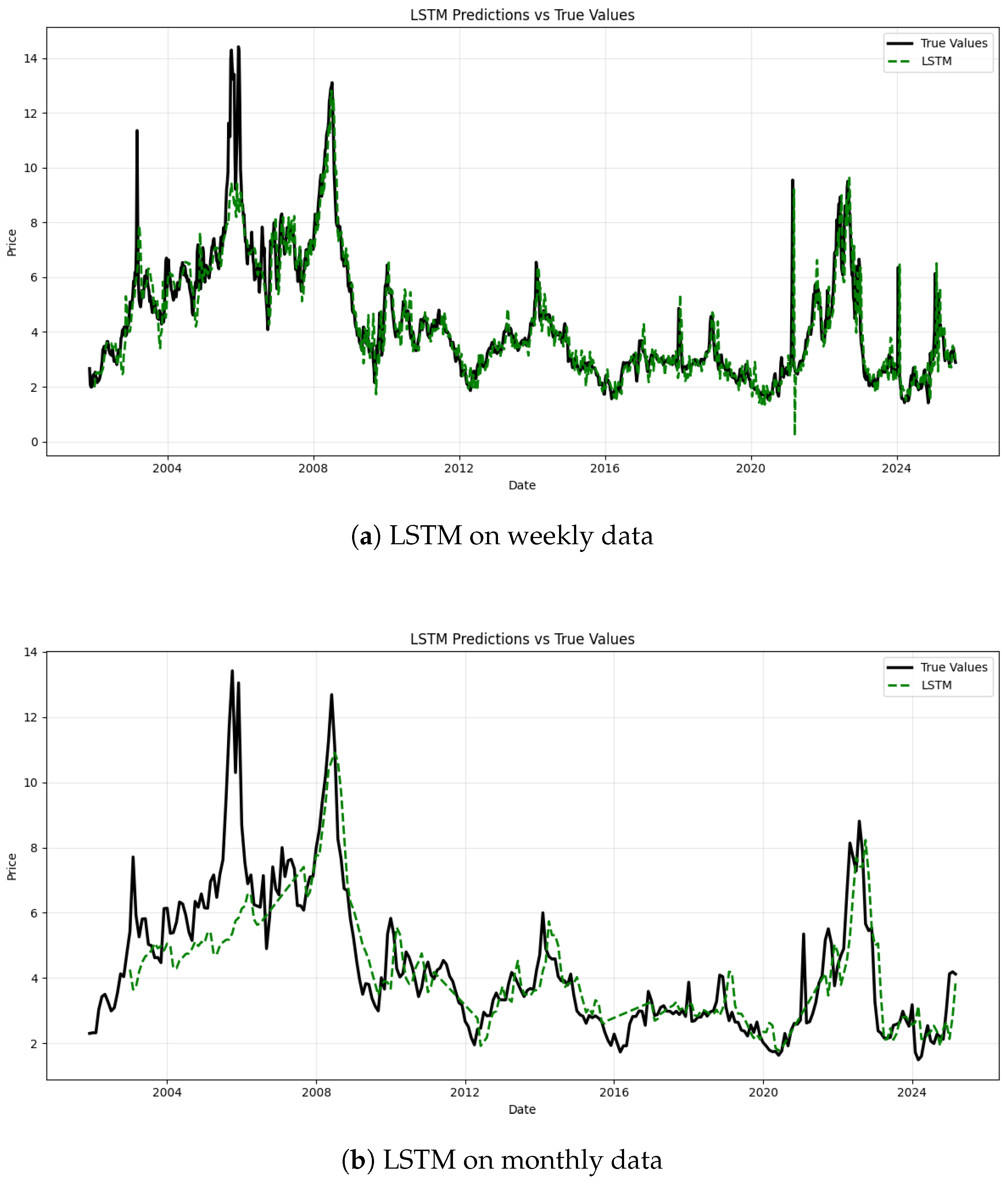
To ensure robust evaluation, a five-fold cross-validation approach is implemented. The resulting fitting curves of the LSTM model across on weekly and monthly data are shown in Figure 6.

As illustrated in Figure 6, the LSTM model’s predicted values demonstrate strong alignment with the observed values in most scenarios, particularly during periods of pronounced price volatility where the model effectively captures the dynamic trends of the actual price trajectory. However, during intervals characterized by extreme price fluctuations, the model exhibits relatively larger prediction errors as evidenced by noticeable discrepancies between the predicted and observed values. This suggests that while the LSTM architecture excels in modeling long-term temporal dependencies within time series data, it demonstrates inherent limitations in accurately forecasting abrupt or extreme market events.

3.4. Comparative Analysis of Forecasting Performance Among Multiple Ensemble Models

To further enhance the predictive performance, three ensemble strategies such as stacking ensemble, bagging ensemble, and weighted average ensemble are employed to integrate the two base models and generate forecasts for the natural gas price series. Each method leverages predictions from multiple base models to produce a more accurate and robust final forecast by reducing model variance and capturing complementary strengths across individual predictors.

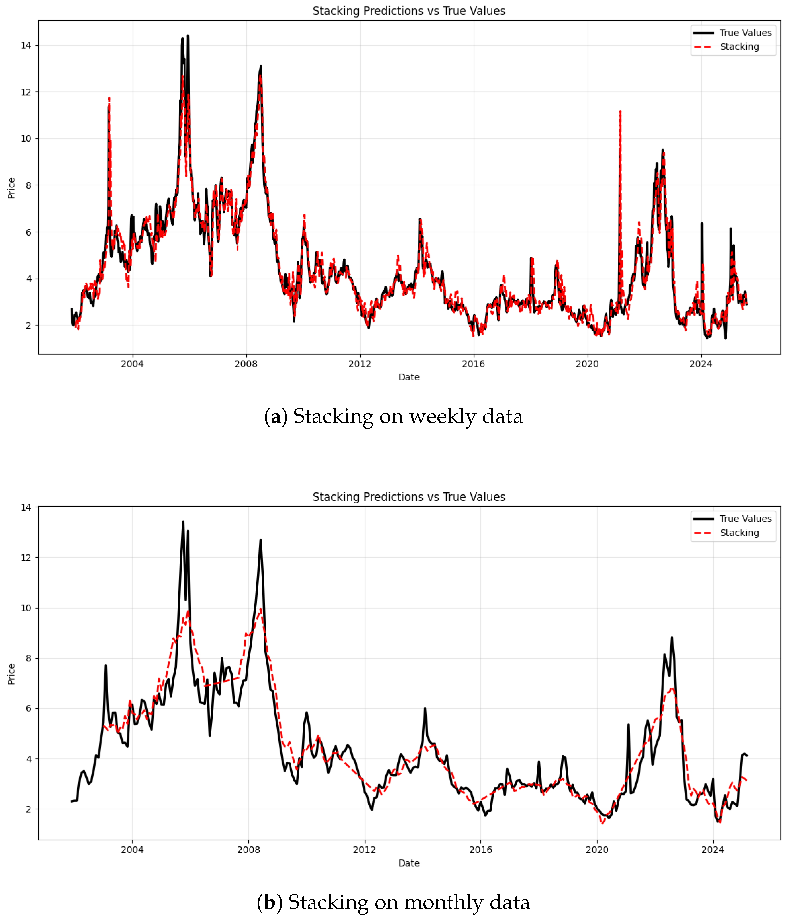
The stacking ensemble method integrates predictions from individual base models by employing a meta-model that learns the optimal combination strategy. In this study, ARIMA (SARIMA) and LSTM models are used as base learners, and their predictions are integrated through Out-of-Fold (OOF) predictions. Specifically, via 5-fold time series cross-validation, predictions for the test set (outer fold data) of each fold are generated independently using ARIMA and LSTM. These outer-fold predictions are then aggregated and used as input features, termed meta-features, for the second-level model. A meta-model is trained on these meta-features along with their corresponding true target values; importantly, these target values are from samples not used in training the base models. Meanwhile, a linear regression model is selected as the meta-model with MSE loss optimized via ordinary least squares (OLS), and trained on OOF predictions. This ensures the meta-model is trained on outer-fold prediction results and their corresponding true targets (rather than samples that the base models are trained on), thus preventing the meta-model from being exposed to target values of training samples that the base models might have overfitted to. During inference, the base models generate predictions that are stacked and fed into the meta-model to produce the final ensemble output, which is formulated as

$${\widehat{y}}_t^{\mathrm{stacking}}=f_{\mathrm{meta}}\left({\widehat{y}}_t^{\left(1\right)},{\widehat{y}}_t^{\left(2\right)},\dots ,{\widehat{y}}_t^{\left(n\right)}\right),$$

where ${\widehat{y}}_t^{\left(i\right)}$ denotes the forecast generated by the $i-th$ base model at time t, and $f_{\mathrm{meta}}$ is the learned meta-model.

To ensure a thorough evaluation, five-fold cross-validation is employed, and the fitting performance results of the stacking ensemble across various datasets are depicted in Figure 7.

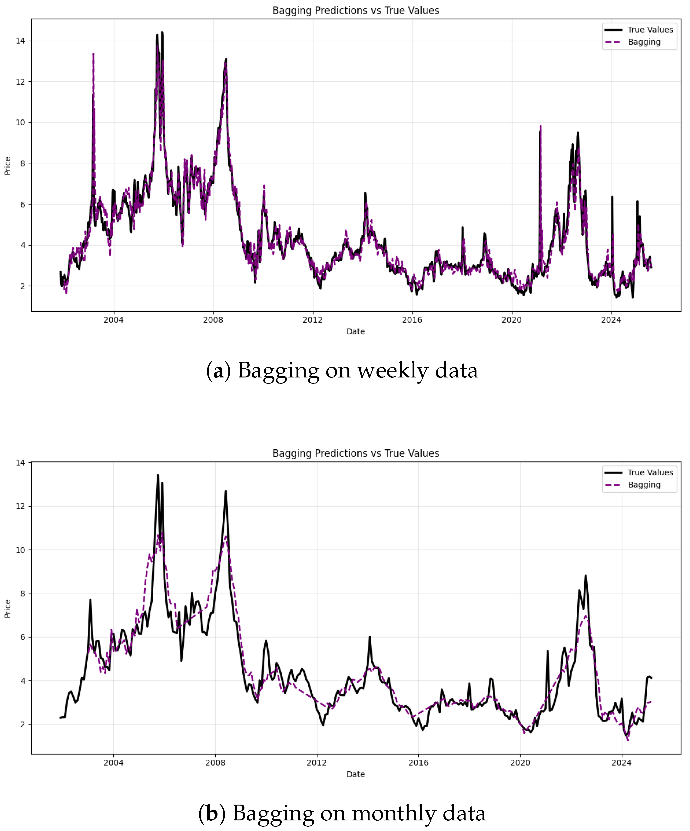
Meanwhile, considering the temporal correlation characteristics of time series data, the bagging ensemble model designed in this study is an upper-level integration framework based on the prediction results of base models. It takes the prediction results of ARIMA (SARIMA) and LSTM as meta-features. Firstly, through time index alignment, the common temporal samples between the predictions of these two types of base models and the true values are filtered out to construct a meta-feature matrix with dimensions (number of samples × 2). Subsequently, the Moving Block Bootstrap (MBB) resampling strategy is adopted with a block size of 8 for weekly data and 6 for monthly data, where 10 groups of differentiated resampled training sets are generated by randomly extracting and concatenating continuous temporal blocks. Each resampled set independently trains a linear regression base learner, ultimately forming a bagging ensemble pool consisting of 10 base learners. In the prediction phase, the ARIMA and LSTM predictions of the samples to be predicted are input into all base learners, and the final prediction value of the bagging ensemble is obtained by taking the temporal average of the outputs from each base learner, which can be expressed as

$${\widehat{y}}_t^{\mathrm{bagging}}={\displaystyle \frac{1}{N}}\sum _{i=1}^N{\widehat{y}}_t^{\left(i\right)},$$

This construction method not only preserves the intrinsic correlation of time series through moving block resampling but also reduces the variance of individual models by leveraging the differentiated predictions of multiple base learners. It effectively avoids the impact of overfitting in base models on the ensemble results and enhances the stability and generalization ability of time series prediction. The corresponding prediction performance is visualized in Figure 8.

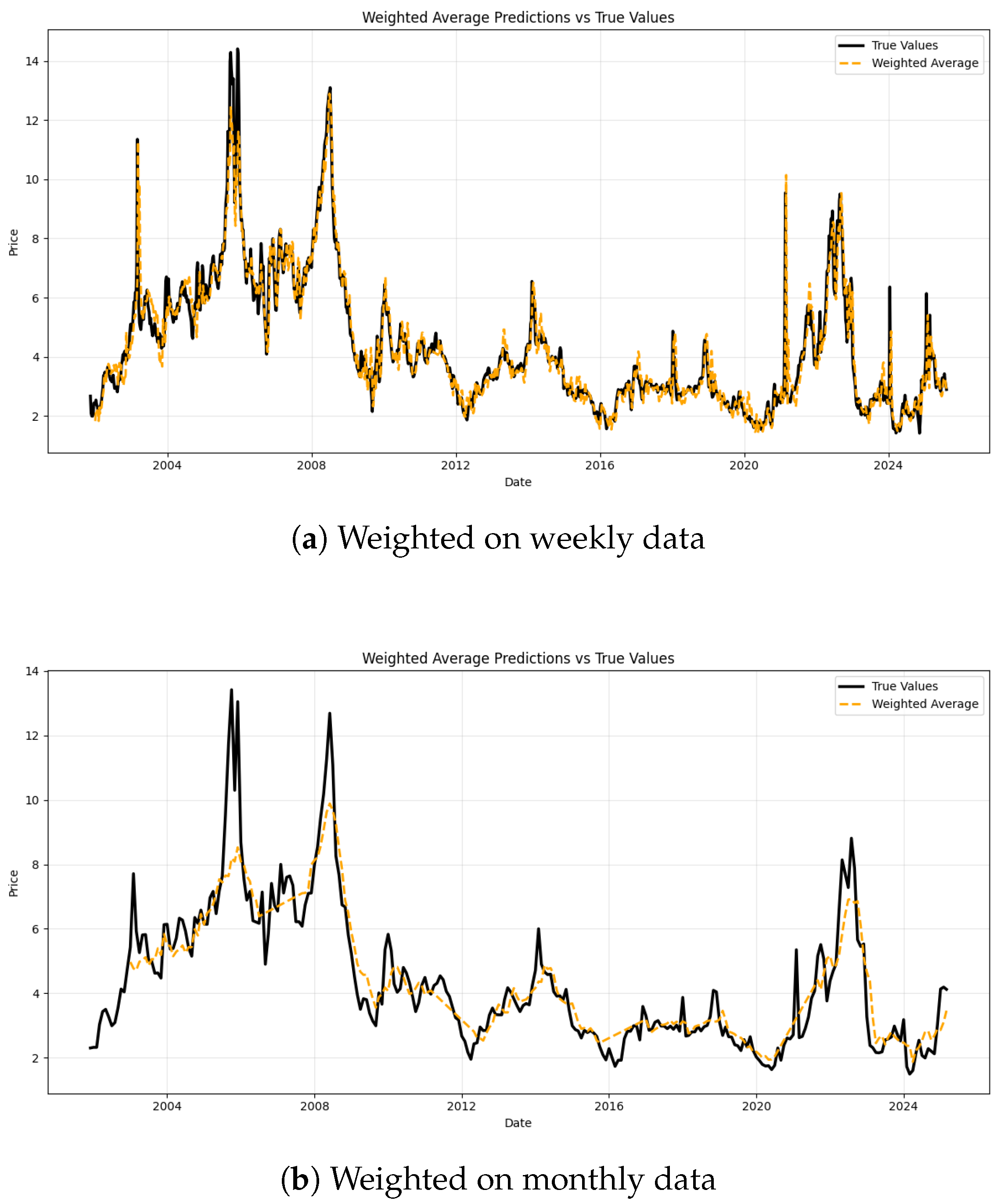
Finally, the weighted average ensemble method combines forecasts from two distinct models such as ARIMA or SARIMA with the LSTM model, based on their relative predictive performance. Specifically, model weights are determined according to the inverse of each model’s MAE on the validation set such that models exhibiting superior accuracy are assigned higher weights, formulated as

$$w_i={\displaystyle \frac{1/{\mathrm{MAE}}_i}{{\sum }_j(1/{\mathrm{MAE}}_j)}},$$

where the weight assigned to model i, and $MA{E}_i$ is its corresponding MAE. Subsequently, the final prediction is computed as the weighted sum of the individual model outputs, given as

$${\widehat{y}}_t^{\mathrm{weighted}}=w^{\mathrm{ARIMA}\mathrm{or}\mathrm{SARIMA}}·{\widehat{y}}_t^{\mathrm{ARIMA}\mathrm{or}\mathrm{SARIMA}}+w^{\mathrm{LSTM}}·{\widehat{y}}_t^{\mathrm{LSTM}}.$$

This strategy combines diverse forecasting techniques with the model’s performance and is illustrated in Figure 9.

From the above prediction fitting figures, it can be seen that the bagging method has the best prediction effect, indicating that this method can effectively integrate the advantages of the two base models and improve the accuracy and robustness of prediction.

To facilitate a direct comparison between individual and ensemble models,

Table 6. Results of model error metrics on weekly data.

	ARIMA	LSTM	Stacking	Bagging	Weighted Average
MAPE (%)	11.01	11.52	9.67	9.60	9.69
MAE	0.4259	0.4995	0.3976	0.3865	0.4022
RMSE	0.6707	0.7632	0.6008	0.5780	0.6016
$R^2$	0.7440	0.7211	0.8031	0.8287	0.8050

presents the computed performance metrics for ARIMA, LSTM, and the ensemble approach on weekly data.

As seen from Table 6, during the weekly data, the ensemble approach outperforms the individual base models in terms of predictive accuracy. Among the three ensemble methods evaluated, the bagging ensemble achieves the lowest MAPE, MAE, and RMSE, as well as the highest $R^2$. This result indicates that the bagging approach outperforms both the stacking and weighted average ensembles in terms of forecasting accuracy.

Moreover, to facilitate a direct comparison between individual and ensemble models,

Table 7. Results of model error metrics on monthly data.

	ARIMA	SARIMA	LSTM	Stacking	Bagging	Weighted Average
MAPE (%)	12.14	12.12	18.41	11.87	11.43	12.47
MAE	0.5261	0.5253	0.8670	0.5570	0.5302	0.5718
RMSE	0.7154	0.7145	1.1812	0.7294	0.6944	0.7978
$R^2$	0.7698	0.7702	0.3196	0.7531	0.7813	0.7089

presents the computed performance metrics for ARIMA, SARIMA, LSTM, and the ensemble approach on monthly data.

As seen from Table 7, the ensemble approach slightly outperforms the individual base models in terms of predictive accuracy. During the monthly data, based on the comparison of error metrics between the ARIMA and SARIMA models, the SARIMA and LSTM models are selected for ensemble modeling. On the weekly data, the bagging ensemble method slightly outperforms other models in terms of MAPE of 9.60%, MAE of 0.3865, RMSE of 0.5780, and $R^2$ of 0.8287. Similarly, on the monthly data, the bagging ensemble method also slightly outperforms other models in terms of MAPE of 11.43%, MAE of 0.5302, RMSE of 0.6944, and $R^2$ of 0.7813. Specifically, among the three ensemble methods evaluated for both weekly and monthly data, the bagging ensemble performs slightly better. This result indicates that the bagging approach slightly outperforms both the stacking and weighted average ensembles in terms of forecasting accuracy.

4. Conclusions and Discussion

To develop a more accurate ensemble method for natural gas price forecasting across time scales while considering model complexity and computational cost, this paper compares two ensemble models. One combines ARIMA optimized through 5-fold cross-validation and LSTM for weekly data, and the other integrates LSTM with the better-performing model between ARIMA and SARIMA, where the better-performing one is selected via error metrics, for monthly data. Both of these ensemble models use STL decomposition to separate seasonal, trend, and residual components: ARIMA and LSTM capture linear patterns, and LSTM models residual nonlinear dependencies. This paper also evaluates stacking, bagging, and weighted averaging to find the optimal hybrid approach.

Despite the contributions of this study, several limitations should be acknowledged. Firstly, the analysis relies exclusively on a single dataset without incorporating regional variations, potentially limiting the generalizability of the findings. Secondly, external factors such as macroeconomic indicators, weather patterns, and geopolitical events are not integrated into the modeling framework, which may overlook critical drivers of natural gas price fluctuations. Thirdly, the absence of nonlinear meta-learners such as gradient boosting machines or neural network-based ensemblers prevent further refinement of the ensemble framework due to data constraints. Finally, this study does not explicitly account for the impacts of market-specific characteristics (e.g., storage capacity and regulatory policies) on model performance.

To address these limitations in future research, two key directions could be prioritized. On the one hand, future research should thus validate the proposed framework by expanding the dataset: collect multi-regional and multi-temporal natural gas price data, and integrate external variables such as economic indices and climate factors to capture broader market interactions and thereby better assess its cross-market robustness. On the other hand, diversifying the ensemble framework through the development of additional base models and optimization of their combinations enhances predictive accuracy via complementary modeling strengths. These improvements could ultimately lead to more robust and universally applicable forecasting methodologies.

Research on improving the efficiency of natural gas price forecasting models facilitates timely policy formulation by governments and contributes to the support of sustainable development goals. This paper presents a comparative analysis of ensemble models for natural gas price forecasting at two temporal scales such as weekly and monthly. The findings lead to the following conclusions. On the weekly dataset, the bagging ensemble method demonstrates a marginal edge over other models, with a MAPE of 9.60%, MAE of 0.3865, RMSE of 0.5780, and an R² of 0.8287. Meanwhile, on the monthly dataset, the bagging ensemble maintains this slight superiority, achieving a MAPE of 11.43%, MAE of 0.5302, RMSE of 0.6944, and an R² of 0.7813. The results demonstrate that the bagging ensemble method slightly outperforms the other two ensemble approaches in predictive accuracy on both temporal scales. This finding highlights the robustness and effectiveness of the bagging framework across different data frequencies, can aid risk management by enabling traders and firms to hedge against price uncertainty, suggests potential patterns consistent with the nuances of the semi-strong efficient market hypothesis to integrate with market efficiency theory, and supports cost structure optimization in the industry by predicting input cost volatility. We also link forecast accuracy to broader macroeconomic stability and market dynamics, providing a valuable reference for future energy price forecasting research.

References

1. Blanchard, O.; Gali, J. Real wage rigidities and the New Keynesian model. J. Money Credit Bank. 2007, 39, 35–65. [Google Scholar] [CrossRef]
2. Kilian, L. The economic effects of energy price shocks. J. Econ. Lit. 2008, 46, 871–909. [Google Scholar] [CrossRef]
3. Fama, E.F. Efficient capital markets: A review of theory and empirical work. J. Financ. 1970, 25, 383–417. [Google Scholar] [CrossRef]
4. Mouchtaris, D.; Sofianos, E.; Gogas, P.; Papadimitriou, T. Forecasting natural gas spot prices with machine learning. Energies 2021, 14, 5782. [Google Scholar] [CrossRef]
5. Li, M.; Kong, Y. Prediction of Natural Gas Price Based on Time Series Model. Pet. New Energy 2023, 35, 61–66. [Google Scholar]
6. Su, M.; Zhang, Z.; Zhu, Y.; Zha, D.; Wen, W. Data Driven Natural Gas Spot Price Prediction Models Using Machine Learning Methods. Energies 2019, 12, 1680. [Google Scholar] [CrossRef]
7. Bilgili, M.; Pinar, E. Gross electricity consumption forecasting using LSTM and SARIMA approaches: A case study of Türkiye. Energy 2023, 284, 128575. [Google Scholar] [CrossRef]
8. Kim, K.; Lim, S.; Lee, W.J.; Jeon, H.; Jung, J.; Jung, D. Forecasting Liquefied Natural Gas Bunker Prices Using Artificial Neural Network for Procurement Management. J. Mar. Sci. Eng. 2022, 10, 1814. [Google Scholar] [CrossRef]
9. He, K.; Ji, L.; Wu, C.W.D.; Tso, K.F.G. Using SARIMA–CNN–LSTM approach to forecast daily tourism demand. J. Hosp. Tour. Manag. 2021, 49, 25–33. [Google Scholar] [CrossRef]
10. Parasyris, A.; Alexandrakis, G.; Kozyrakis, G.V.; Spanoudaki, K.; Kampanis, N.A. Predicting meteorological variables on local level with SARIMA, LSTM and hybrid techniques. Atmosphere 2022, 13, 878. [Google Scholar] [CrossRef]
11. Peirano, R.; Kristjanpoller, W.; Minutolo, M.C. Forecasting inflation in Latin American countries using a SARIMA–LSTM combination. Soft Comput. 2021, 25, 10851–10862. [Google Scholar] [CrossRef]
12. Tahyudin, I.; Wahyudi, R.; Nambo, H. SARIMA-LSTM Combination for COVID-19 Case Modeling. IIUM Eng. J. 2022, 23, 171–182. [Google Scholar] [CrossRef]
13. Yu, H.; Song, S. Natural Gas Futures Price Prediction Based on Variational Mode Decomposition–Gated Recurrent Unit/Autoencoder/Multilayer Perceptron–Random Forest Hybrid Model. Sustainability 2025, 17, 2492. [Google Scholar] [CrossRef]
14. Choudhary, K.; Jha, G.K.; Jaiswal, R.; Kumar, R.R. A genetic algorithm optimized hybrid model for agricultural price forecasting based on VMD and LSTM network. Sci. Rep. 2025, 15, 9932. [Google Scholar] [CrossRef] [PubMed]
15. Da, X.; Ye, D.; Shen, Y.; Cheng, P.; Yao, J.; Wang, D. A novel hybrid method for multi-step short-term 70 m wind speed prediction based on modal reconstruction and STL-VMD-BiLSTM. Atmosphere 2024, 15, 1014. [Google Scholar] [CrossRef]
16. Li, X.; Zou, X.; Cheng, J.; Tang, M.; Hu, P. FMM-VMD-Transformer: A hybrid deep learning model for predicting natural gas consumption. Digit. Eng. 2024, 2, 100005. [Google Scholar] [CrossRef]
17. Kumar, I.; Tripathi, B.K.; Singh, A. Attention-based LSTM network-assisted time series forecasting models for petroleum production. Eng. Appl. Artif. Intell. 2023, 123, 106440. [Google Scholar] [CrossRef]
18. Jiang, H.; Hu, W.; Lao, L.; Dong, Y. A decomposition ensemble based deep learning approach for crude oil price forecasting. Resour. Policy 2022, 78, 102855. [Google Scholar] [CrossRef]
19. Wu, Z.; Zhou, J.; Yu, X. Forecast Natural Gas Price by an Extreme Learning Machine Framework Based on Multi-Strategy Grey Wolf Optimizer and Signal Decomposition. Sustainability 2025, 17, 5249. [Google Scholar] [CrossRef]
20. Abdellatif, A.; Mubarak, H.; Ahmad, S.; Ahmed, T.; Shafiullah, G.M.; Hammoudeh, A.; Abdellatef, H.; Rahman, M.M.; Gheni, H.M. Forecasting Photovoltaic Power Generation with a Stacking Ensemble Model. Sustainability 2022, 14, 11083. [Google Scholar] [CrossRef]
21. Nguyen, H.V.; Byeon, H. Prediction of Parkinson’s Disease Depression Using LIME-Based Stacking Ensemble Model. Mathematics 2023, 11, 708. [Google Scholar] [CrossRef]
22. Li, Z.; Zhao, N.; Zhang, H.; Wei, Y.; Chen, Y.; Ma, R. Research on High Spatiotemporal Resolution of XCO2 in Sichuan Province Based on Stacking Ensemble Learning. Sustainability 2025, 17, 3433. [Google Scholar] [CrossRef]
23. Duan, Y.; Zhang, J.; Wang, X. Henry Hub Monthly Natural Gas Price Forecasting Using CEEMDAN–Bagging–HHO–SVR. Front. Energy Res. 2023, 11, 1323073. [Google Scholar] [CrossRef]
24. Adnan, R.M.; Jaafari, A.; Mohanavelu, A.; Kisi, O.; Elbeltagi, A. Novel Ensemble Forecasting of Streamflow Using Locally Weighted Learning Algorithm. Sustainability 2021, 13, 5877. [Google Scholar] [CrossRef]
25. Wang, J.; Lei, C.; Guo, M. Daily natural gas price forecasting by a weighted hybrid data-driven model. J. Pet. Sci. Eng. 2020, 192, 107240. [Google Scholar] [CrossRef]
26. Shashvat, K.; Basu, R.; Bhondekar, A.P.; Kaur, A. A weighted ensemble model for prediction of infectious diseases. Curr. Pharm. Biotechnol. 2019, 20, 674–678. [Google Scholar] [CrossRef]
27. Abdollahi, H. A novel hybrid model for forecasting crude oil price based on time series decomposition. Appl. Energy 2020, 267, 115035. [Google Scholar] [CrossRef]
28. Guo, F.; Mo, H.; Wu, J.; Pan, L.; Zhou, H.; Zhang, Z.; Huang, F. A hybrid stacking model for enhanced short-term load forecasting. Electronics 2024, 13, 2719. [Google Scholar] [CrossRef]
29. Yu, L.; Dai, W.; Tang, L. A novel decomposition ensemble model with extended extreme learning machine for crude oil price forecasting. Eng. Appl. Artif. Intell. 2016, 47, 110–121. [Google Scholar] [CrossRef]
30. Ye, P.; Li, Y.; Siddik, A.B. Forecasting the return of carbon price in the Chinese market based on an improved stacking ensemble algorithm. Energies 2023, 16, 4520. [Google Scholar] [CrossRef]
31. Zhou, Y.; Li, T.; Shi, J.; Qian, Z. A CEEMDAN and XGBOOST-based approach to forecast crude oil prices. Complexity 2019, 2019, 4392785. [Google Scholar] [CrossRef]
32. Wang, J.; Cao, J.; Yuan, S.; Cheng, M. Short-term forecasting of natural gas prices by using a novel hybrid method based on a combination of the CEEMDAN-SE-and the PSO-ALS-optimized GRU network. Energy 2021, 233, 121082. [Google Scholar] [CrossRef]
33. Yun, P.; Huang, X.; Wu, Y.; Yang, X. Forecasting carbon dioxide emission price using a novel mode decomposition machine learning hybrid model of CEEMDAN-LSTM. Energy Sci. Eng. 2023, 11, 79–96. [Google Scholar] [CrossRef]
34. Gangwar, S.; Bali, V.; Kumar, A. Comparative Analysis of Wind Speed Forecasting Using LSTM and SVM. EAI Endorsed Trans. Scalable Inf. Syst. 2020, 7, 25. [Google Scholar] [CrossRef]
35. Li, R.; Song, X. A multi-scale model with feature recognition for the use of energy futures price forecasting. Expert Syst. Appl. 2023, 211, 118622. [Google Scholar] [CrossRef]
36. Szostek, K.; Mazur, D.; Drałus, G.; Kusznier, J. Analysis of the Effectiveness of ARIMA, SARIMA, and SVR Models in Time Series Forecasting: A Case Study of Wind Farm Energy Production. Energies 2024, 17, 19. [Google Scholar] [CrossRef]
37. Box, G.E.P.; Jenkins, G.M. Time Series Analysis: Forecasting and Control, 1st ed.; Holden-Day: San Francisco, CA, USA, 1976. [Google Scholar]
38. Hochreiter, S.; Schmidhuber, J. Long Short-Term Memory. Neural Comput. 1997, 9, 1735–1780. [Google Scholar] [CrossRef]
39. Qiu, X. Neural Networks and Deep Learning; China Machine Press: Beijing, China, 2020; pp. 145–147. [Google Scholar]
40. Henry Hub Trading Center. 2025. Available online: https://www.eia.gov/dnav/ng/hist/rngwhhdM.htm (accessed on 10 August 2025).
41. Cleveland, R.B.; Cleveland, W.S. STL: A Seasonal-Trend Decomposition Procedure Based on Loess. J. Off. Stat. 1990, 6, 3–33. [Google Scholar]
Figure 1. Recurrent unit structure of an LSTM network.
Sustainability 17 08514 g001
Figure 2. Original natural gas price time series at different temporal scales.
Sustainability 17 08514 g002
Figure 3. Decomposition result diagram: (a,b) display the seasonal components, (c,d) illustrate the trend components, and (e,f) show the residual components.
Sustainability 17 08514 g003
Figure 4. Autocorrelation and partial autocorrelation functions: (a,b) show the ACF for weekly and monthly data, respectively; (c,d) present the PACF patterns.
Sustainability 17 08514 g004
Figure 5. Comparison of predicted and actual natural gas prices.
Sustainability 17 08514 g005
Figure 6. Comparison of predicted and actual natural gas prices.
Sustainability 17 08514 g006
Figure 7. Comparison of predicted and actual natural gas prices.
Sustainability 17 08514 g007
Figure 8. Comparison of predicted and actual natural gas prices.
Sustainability 17 08514 g008
Figure 9. Comparison of predicted and actual natural gas prices.
Sustainability 17 08514 g009