Advanced Machine Learning Methods as a Planning Strategy in the Capellanía Wetland

Abstract

This study evaluated the spatio-temporal dynamics of vegetation cover in the Capellanía wetland (Bogotá, Colombia) between 2013 and 2032 through spectral indices, machine learning, and spatial simulation. A multitemporal Random Forest model (R² = 0.991; RMSE = 0.0214; MAE = 0.0127) was integrated with cellular automata (MOLUSCE) to project vegetation trajectories under different urban growth scenarios. NDVI-based classification revealed a marked transition: degraded classes (bare soil and sparse vegetation) decreased from over 80% in 2013 to less than 10% in 2032, while moderate and dense vegetation surpassed 90%. Cellular automata achieved moderate agreement (Kappa = 0.640) and high internal calibration (pseudo-R² = 1.00); the transition matrix in scenario II, simulating the construction of the Avenida Longitudinal de Occidente (ALO), indicated a conversion 0→1 = 0.414 and persistence 1→1 = 0.709, evidencing intense urbanization pressure in peripheral areas. The Shannon index confirmed recovery but highlighted structural homogenization, underscoring the need to preserve heterogeneity to sustain ecosystem resilience. Scenario analysis showed that the ALO would act as a catalyst for urban expansion, threatening ecological connectivity and increasing pressure on vegetation. Overall, this study provides quantitative, spatial, and prospective evidence to promote preventive, integrated, and data-driven approaches for the conservation of strategic urban wetlands.

1. Introduction

Wetlands are strategic ecosystems that play a crucial role in maintaining biodiversity and hydromorphic vegetation. They function as natural buffers against floods, filter pollutants, and provide habitat for endemic species. However, accelerated urban growth has transformed these ecosystems, leaving only small remnants within highly urbanized zones [1]. In addition, planning policies and road construction have fragmented wetlands, reducing vegetation cover, water bodies, and, consequently, the resilience of these ecosystems [2].

In Latin America and the Caribbean, wetlands located within or near cities are highly threatened by rapid population growth and informal settlements that invade hydraulic buffer zones and areas designated for environmental management [3]. Weaknesses in territorial planning and public policy exacerbate their degradation, with impacts not only on ecological processes but also on economic activities and spatial organization. As a result, mangroves, lagoons, and marshes have suffered severe transformations due to their proximity to large urban centers [4]. For example, in Lima (Peru), 203 hectares of wetlands disappeared between 1990 and 2013, compromising their ecological functions. In Chile, the Aconcagua–Concón wetland has been deteriorating since 2015 due to urban pressure and extreme climatic events [5].

In this context, photointerpretation and satellite imagery have proven useful for monitoring wetland transformations. Specifically, the Normalized Difference Vegetation Index (NDVI), derived from near-infrared and visible red bands, has been widely applied to classify land cover and distinguish natural from artificial zones [6]. NDVI provides a powerful tool for regional-scale monitoring, given the accessibility of remote sensing data and its applicability across diverse Latin American contexts.

Similarly, spectral water indices are essential for detecting water bodies and quantifying surface moisture based on reflectance in near-, mid-, and shortwave infrared bands [6,7]. Among them, the Normalized Difference Water Index (NDWI) is widely used in wetland studies. For instance, urban wetlands in China have been analyzed with NDWI to assess water body variations under anthropogenic and climatic influences [8]. In Colombia, Pedraza et al. [9] used NDWI to track seasonal water fluctuations in the Torca–Guaymaral wetland, while in Kenya, the Automated Water Extraction Index (AWEI) has been applied to analyze historical water-level variations in Lake Baringo, incorporating factors such as land use change, surface temperature, erosion, sedimentation, and precipitation [3].

More recently, the integration of spectral indices with advanced machine learning (ML) methods has expanded monitoring and predictive capacities. Algorithms such as Random Forest (RF) and cellular automata (CA) allow for the simulation of land-use dynamics at the pixel level, capturing spatiotemporal processes of change. Random Forest stands out for its robustness against noise, ability to handle high-dimensional datasets, and capacity to evaluate variable importance. When combined with neural networks—particularly for calibrating transition rules—ML methods achieve high accuracy in projecting future scenarios [10].

The integration of these spectral indices with advanced machine learning (ML) methods has significantly expanded monitoring and predictive capacities. Algorithms such as Random Forest (RF) are particularly notable for their robustness against noise, ability to handle high-dimensional datasets, and capacity to evaluate variable importance. For example, the RF algorithm has been successfully employed using vegetation indices to classify wetlands and create classification maps in Gansu Province across eight periods from 1987 to 2020 (at 30 m resolution), achieving robust results with an average overall accuracy (OA) of 96.0% and a Kappa coefficient of 0.954 [11]. The marsh wetland type exhibited the highest average user’s accuracy (UA) and producer’s accuracy (PA) at 96.4% and 95.2%, respectively. When combined with other techniques like cellular automata (CA)—particularly using neural networks for calibrating transition rules—these ML methods achieve high accuracy in projecting future scenarios [10,12].

Several studies illustrate the effectiveness of this approach in wetland conservation. At Khinjhir Lake, Pakistan, a spatiotemporal analysis (2000–2020) combining spectral indices, Random Forest, and CA–Markov modeling revealed an 11% reduction in water bodies and a 30% loss of moderately to highly vulnerable zones, with projections indicating further decline [13]. Likewise, in Cauca, Colombia, the application of K-Means and Random Forest with NDVI/NDWI enabled the identification of five wetland complexes, including 25,929.39 ha of high-vegetation swamps and 1795.51 ha of low-vegetation cover [14].

In Bogotá, the urgency of such approaches is clear: wetlands have lost 84.52% of their area in the 21st century due to urban growth and road infrastructure development [15]. The Capellanía wetland, despite being part of Bogotá’s Main Ecological Structure and receiving international protection under the Ramsar Convention, remains highly vulnerable. Infrastructure projects, such as Avenida La Esperanza and Avenida Ferrocarril de Occidente, have already fragmented its connectivity, while the planned Avenida Longitudinal de Occidente (ALO) threatens to eliminate nearly one-third of its area, severely affecting its hydrological dynamics and vegetation [16].

Given this situation, the present study seeks to monitor the Capellanía wetland using spectral indices and machine learning algorithms to predict future scenarios and evaluate vegetation cover changes under urban expansion pressures.

2. Materials and Methods

2.1. Methodological Framework

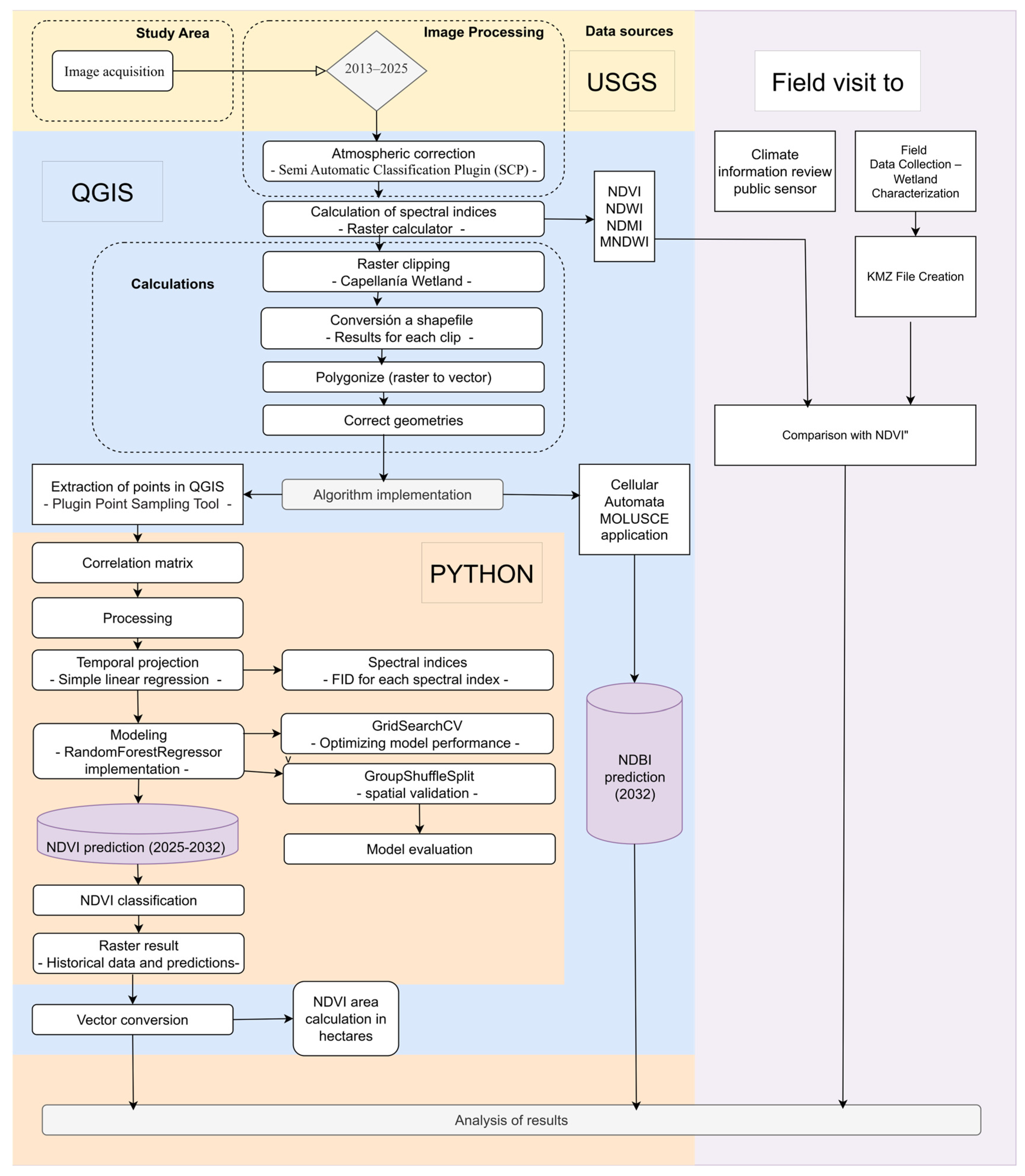
This study analyzes vegetation cover dynamics in the Capellanía wetland through an integrated methodological framework that combines (1) multitemporal remote sensing, (2) fieldwork, (3) spectral index calculation, and (4) predictive modeling with machine learning algorithms. This strategy enabled the quantification of historical vegetation transformation patterns and the projection of future scenarios under varying levels of urban pressure (Figure 1).

Satellite data preprocessing was conducted in QGIS using a standardized workflow that included (1) clipping images to the study area to ensure spatial consistency; (2) converting raster to vector format to obtain discrete spatial units; (3) reclassifying spectral values using correspondence tables and correcting invalid geometries to guarantee topological integrity; and (4) calculating the area of each polygon in hectares to facilitate quantitative analysis.

In parallel, to minimize atmospheric interference, only scenes with minimal cloud cover were selected. This strict quality control of input data was essential to ensure the reliability of subsequent regression analyses and machine learning model training, which included Linear Regression and the Random Forest (RF) algorithm—the latter widely recognized for its robustness in remote sensing applications [16].

2.2. Study Area

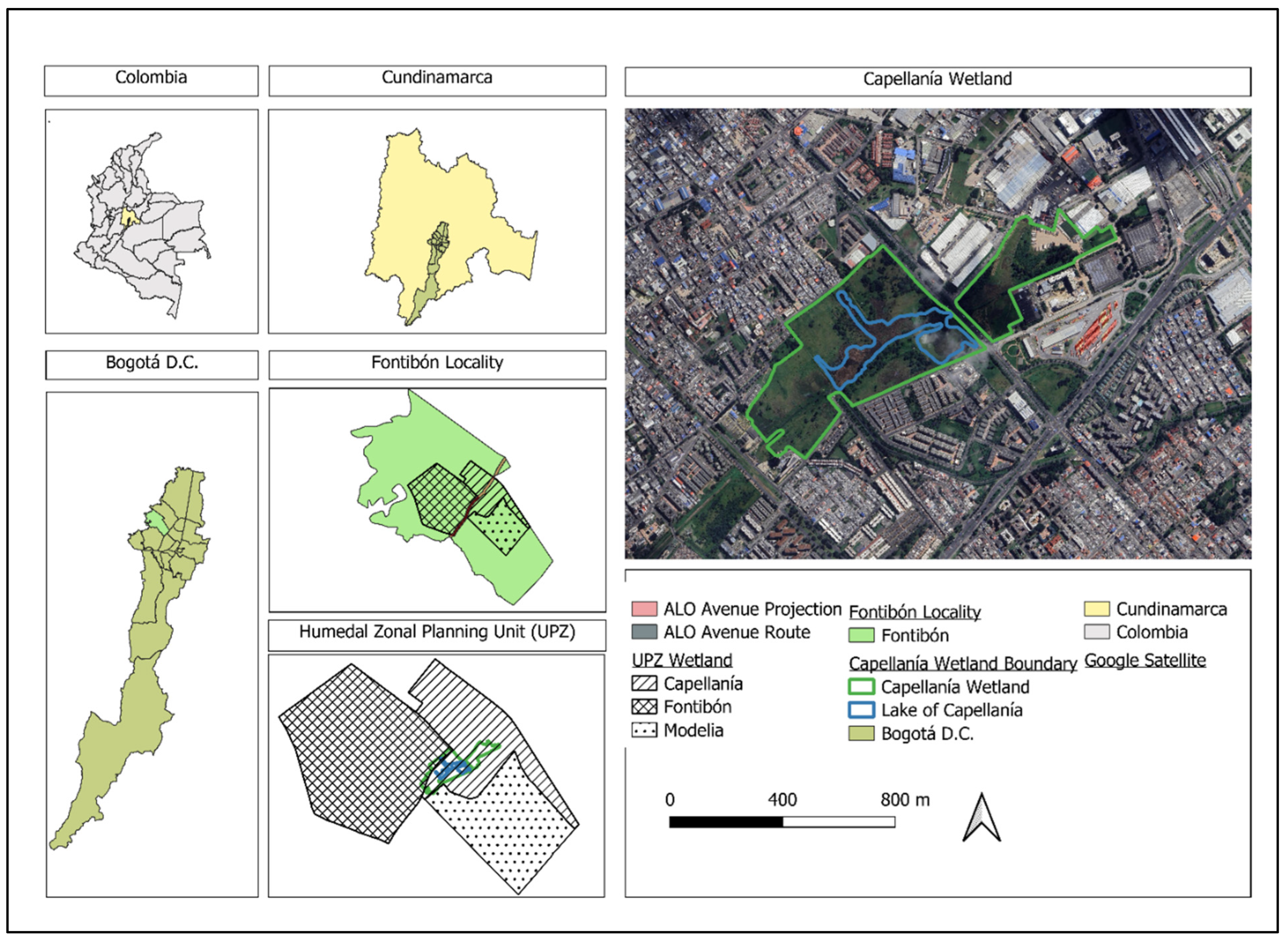
This research was conducted in the Capellanía wetland, located in the northwestern urban sector of Bogotá, within the locality of Fontibón, specifically in the Zonal Planning Units (UPZ) of Modelia, Fontibón Centro, and Capellanía (Figure 2).

∗

The Modelia UPZ covers 261.3 hectares and comprises 5 neighborhoods.

∗

Fontibón Centro UPZ extends over 496.06 hectares with 43 neighborhoods.

∗

The Capellanía UPZ spans 271.8 hectares and includes 6 neighborhoods.

Altogether, the study area encompasses 1029.16 contiguous hectares. The Capellanía wetland itself covers 37.76 hectares, of which 21 hectares are designated as legally protected areas [17]. The study area was selected due to its high vulnerability to urbanization. Historical records indicate that the wetland has lost approximately 88% of its original extent as a result of road infrastructure and urban expansion [18]. Recent studies reinforce this condition, projecting an additional reduction of nearly 25% by 2034 and identifying Capellanía as one of the most impacted urban wetlands in Bogotá [16,19]. This combination of factors makes it a representative case for assessing vegetation dynamics under anthropogenic pressure scenarios.

Climatically, the region exhibits a bimodal rainfall regime with two wet seasons per year (March–June and September–November). August is typically the coldest month, whereas the first two months of the year record the lowest average temperatures. Although this period corresponds to the dry season of the Bogotá Savanna, reduced cloud cover generates strong thermal amplitudes—warm days followed by cold nights—resulting in lower overall mean temperatures [20]. According to the Bogotá Air Quality Monitoring Network, the mean surface temperature in Fontibón over the past 12 years is 14.06 °C [21].

2.3. Field Survey and Land-Cover Identification

The field survey in the Capellanía wetland was conducted in 2024, following standardized methodologies for wetland characterization [15,22]. The protocol involved identifying control points using a high-precision handheld GPS device (Garmin eTrex-30x, Garmin Ltd., Olathe, KS, USA), a widely adopted practice for georeferencing and characterizing vegetation cover [23]. The in situ data collection enabled the registration of coordinates for major vegetation types and water bodies, creating a ground-truth dataset. These observations were essential for verifying vegetation typologies, characterizing landscape elements [24,25], and, critically, validating the results derived from spectral index analysis through remote sensing. The integration of field data and remote sensing is considered a robust approach to improving classification accuracy in wetland ecosystems [26].

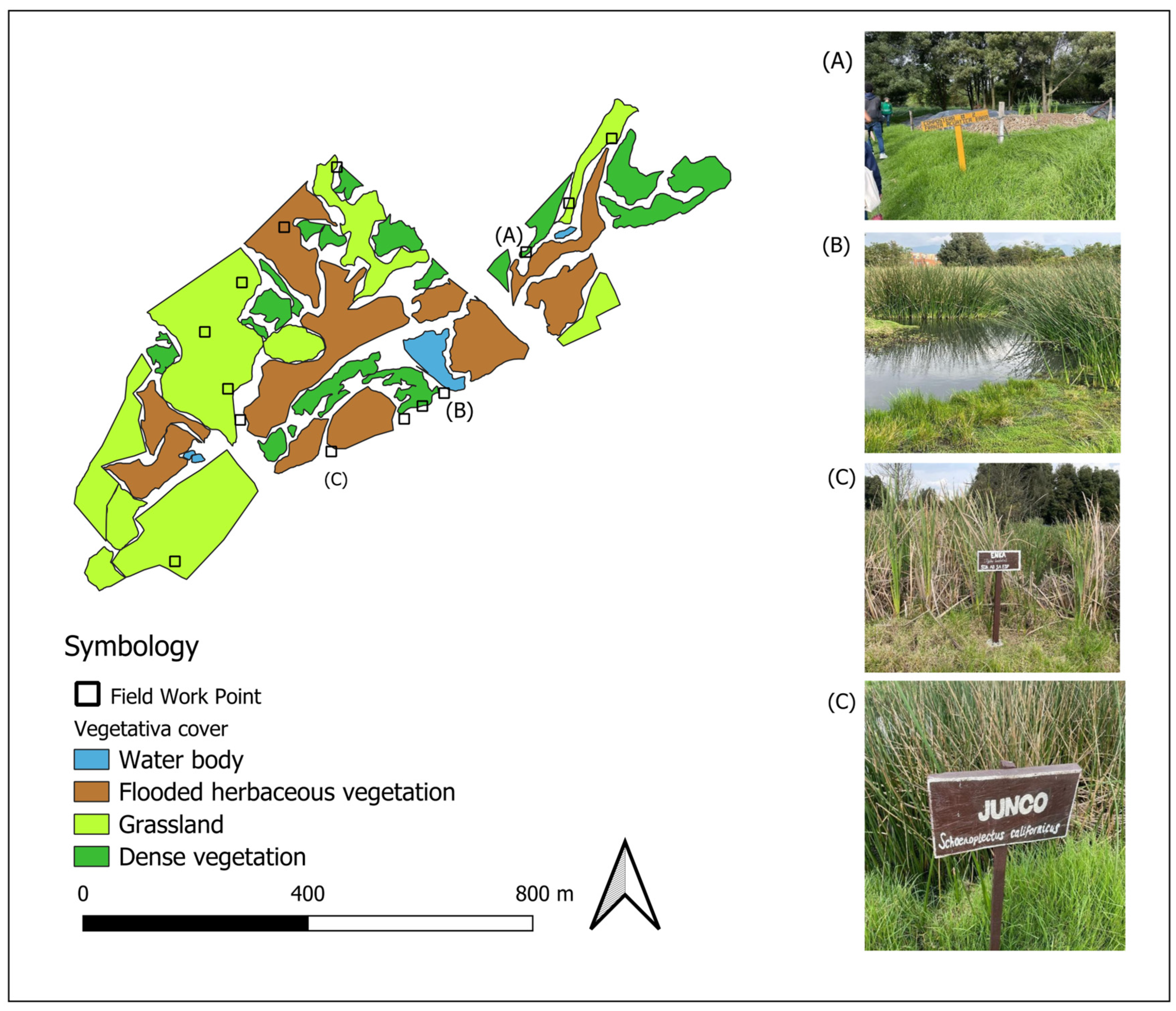
Finally, the collected information was used to generate classified layers in KMZ format, which were subsequently processed in QGIS. As a result of this integrated methodology—combining remote sensing, fieldwork, and GIS analysis—the following land-cover classes were identified and mapped in the study area, using a legend adapted from standardized classification systems such as CORINE Land Cover [27] (Figure 3).

2.4. Spectral Indices in Satellite Image Processing

The first processing stage involved the collection of 35 Landsat 8 images, downloaded from the USGS Earth Explorer platform. Only images with less than 40% cloud cover were selected. Atmospheric correction was applied using the Dark Object Subtraction method (DOS1) through the Semi-Automatic Classification Plugin (SCP) in QGIS [28]. All images were subsequently reprojected to the WGS 84/UTM Zone 18N coordinate system (EPSG:32618) to ensure spatial consistency [29].

The most widely used spectral indices for urban wetlands were calculated: NDVI, NDWI, MNDWI, NDMI, and NDBI, through algebraic operations on specific Landsat 8 bands (

Table 1. Calculation of Spectral Indices for Vegetation, Water, and Urban Areas.

NDVI	NDWI	MNDWI	NDMI	NDBI
${\displaystyle \frac{\mathrm{N}\mathrm{I}\mathrm{R}-\mathrm{R}}{\mathrm{N}\mathrm{I}\mathrm{R}+\mathrm{R}}}$	${\displaystyle \frac{\mathrm{G}\mathrm{r}\mathrm{e}\mathrm{e}\mathrm{n}-\mathrm{N}\mathrm{I}\mathrm{R}}{\mathrm{G}\mathrm{r}\mathrm{e}\mathrm{e}\mathrm{n}+\mathrm{N}\mathrm{I}\mathrm{R}}}$	${\displaystyle \frac{\mathrm{G}\mathrm{r}\mathrm{e}\mathrm{e}\mathrm{n}-\mathrm{S}\mathrm{W}\mathrm{I}\mathrm{R}}{\mathrm{G}\mathrm{r}\mathrm{e}\mathrm{e}\mathrm{n}+\mathrm{S}\mathrm{W}\mathrm{I}\mathrm{R}}}$	${\displaystyle \frac{\mathrm{N}\mathrm{I}\mathrm{R}-\mathrm{S}\mathrm{W}\mathrm{I}\mathrm{R}}{\mathrm{N}\mathrm{I}\mathrm{R}+\mathrm{S}\mathrm{W}\mathrm{I}\mathrm{R}}}$	${\displaystyle \frac{\mathrm{S}\mathrm{W}\mathrm{I}\mathrm{R}-\mathrm{N}\mathrm{I}\mathrm{R}}{\mathrm{S}\mathrm{W}\mathrm{I}\mathrm{R}+\mathrm{N}\mathrm{I}\mathrm{R}}}$

Note: NIR = Near-infrared (Band 5); R = Red (Band 4); Green = Band 3; SWIR = Shortwave infrared (Band 6).

) [3,19]. The combined use of NDVI, NDWI, and MNDWI enhances vegetation detection, water content estimation, and discrimination between water bodies and urban surfaces, thereby increasing classification accuracy in wetland studies [30]. These indices enable the visualization of vegetation dynamics, water body changes, and urban expansion. To assess built-up areas, temporal comparisons were cond for the period 2013–2024.

2.5. Vegetation Reclassification in Remote Sensing

The NDVI thresholds used for classification were established based on widely accepted criteria in the remote sensing literature, which distinguish between surfaces without vegetation cover and those with varying degrees of vegetation density. In this study, four intervals were adopted: bare soil or no vegetation (NDVI < 0.1), sparse vegetation (0.1–0.3), moderate vegetation (0.3–0.5), and dense vegetation (NDVI ≥ 0.5). These thresholds are grounded in the biophysical behavior of NDVI [31], which demonstrates that low NDVI values correspond to bare soil or urban surfaces, whereas higher values indicate vigorous and dense vegetation.

However, since low NDVI values may overlap between water and bare soil, an additional step was introduced to avoid misclassification. Water bodies were identified using water-sensitive spectral indices, particularly the Modified Normalized Difference Water Index (MNDWI), proposed by Xu [30], which improves the delineation of open water bodies in satellite imagery. Thus, water was classified as an independent category, ensuring more accurate separation from non-vegetated soils. The classification thresholds and spectral indices are summarized in

Table 2. Value ranges and spectral indices associated with each reclassification category.

Class	Parameters	NDVI Criteria/Indices
1	Water	(MNDWI > 0) OR (NDWI > 0 AND NDMI < 0)
2	Bare soil/No vegetation	0.0 < NDVI < 0.10
3	Sparse vegetation	0.10 ≤ NDVI < 0.30
4	Moderate vegetation	0.30 ≤ NDVI < 0.50
5	Dense vegetation	NDVI ≥ 0.50

.

2.6. Exploration of Climatic Variables (Not Integrated)

During the exploratory phase, external climatic data (precipitation and temperature) from a nearby station were reviewed. However, these datasets presented limitations in resolution, calibration, and representativeness, which could have introduced noise into the model. Consequently, they were not integrated into the predictive analysis. Previous studies highlight that the accuracy of models such as Random Forest is highly dependent on the quality of input variables, and that climatic data provide meaningful contributions only when derived from reliable in situ observations [32].

For descriptive purposes, correlations were computed between NDVI and the main spectral and climatic variables (NDWI, LST, area, mean temperature, precipitation, and a derived climatic variable). The results indicated weak associations, supporting the decision to exclude them from the predictive modeling (

Table 3. Correlation matrix between NDVI and spectral and climatic variables.

	LST	AVG	PR	PNVin
NDVI	0.2182	0.1948	−0.0944	0.0436

Note: LST: Land Surface Temperature; AVG T: Monthly Average Temperature (°C); PR: Monthly Precipitation (mm); PNVin: Derived Climatic Variable (Precipitation Normalized Linked).

).

2.7. Modeling and Simulation of Future Scenarios

The modeling combined three analytical approaches, ranging from temporal projection using linear regression, vegetation cover estimates, and urban expansion simulations up to 2032, as described below.

2.7.1. Projection of Predictor Variables

Observation dates were transformed into ordinal values, and a future date was established. Using the forecast_index_by_fid function, independent linear models were fitted for each polygon (fid) with at least two records, projecting NDWI, NDMI, and MNDWI values. This procedure allowed the extension of the time series to the analysis horizon and ensured the continuity of the predictors. Although this method assumes an approximately linear relationship over the analyzed period (2013–2024), potentially underestimating non-linear behaviors associated with climatic events or anthropogenic interventions, its application is appropriate given the limited number of observations per polygon and the need to obtain continuous values to feed the main model. This approach has been employed in previous studies on wetland and landscape dynamics [33]. Integration with subsequent non-linear models (such as Random Forest) mitigates this limitation and has been validated in studies of landscape and wetland dynamics [34].

2.7.2. Estimation Using Random Forest

NDVI was used as the dependent variable, while NDWI, NDMI, MNDWI, and seasonal variables (sine and cosine of the month) were used as predictors. These seasonal variables capture the cyclical nature of the calendar and climatic seasonality, representing each month in a unit circular space using trigonometric transformations (month_sin = sin(2π·month/12), month_cos = cos(2π·month/12)). This procedure prevents December and January from appearing artificially distant on a linear scale and allows the model to adequately capture periodic vegetation patterns. In recent studies on Landsat time series, sine and cosine coefficients have proven to be key predictors for describing seasonality and improving vegetation type discrimination compared to conventional seasonal compositions [35].

The dataset was partitioned into 80% for training and 20% for spatial validation using GroupShuffleSplit, ensuring independence between polygons (fid). This strategy prevents the same polygon from appearing in both sets, providing a more robust spatial evaluation. The use of grouped or spatial validation methods has been recommended in recent studies, as random validation can overestimate Random Forest predictive performance in the presence of spatial autocorrelation, whereas block- or group-based approaches more realistically reflect generalization capacity [36].

A Random Forest Regressor with 600 trees was trained, and its hyperparameters were optimized using exhaustive search (GridSearchCV). Model performance was evaluated using accuracy metrics such as R², RMSE, and MAE. This approach aligns with recent research, in which Random Forest, combined with spectral indices and variable optimization, has shown high accuracy in wetland classification (OA > 95%) using Landsat imagery [11].

2.7.3. Thematic Classification and Raster Generation

Thematic classification was performed following the methodology described in Section 2.5, uniformly applying the same NDVI thresholds and water mask. This procedure was replicated for both historical data and projections, generating comparable maps throughout the analysis period. The final output consisted of thematic rasters integrating five categories into a single spatial layer. NDVI predictions and the water mask were joined to the reference vector grid (fid) and subsequently rasterized using the extent and resolution of a base raster in QGIS. This produced projected NDVI maps, water masks, and a final five-class classification, forming the basis for multitemporal analysis and scenario evaluation. A similar methodological approach was used by Suir et al. [37], who applied NDVI thresholds in coastal ecosystems to differentiate vegetation absence, sparse, moderate, and dense vegetation, demonstrating the method’s efficacy in characterizing vegetation vigor and density.

2.7.4. Urban Expansion Simulation with MOLUSCE (QGIS)

Urbanization scenarios were evaluated using the MOLUSCE plugin (Modules for Land Use Change Evaluation) in QGIS, which applies cellular automata to simulate land cover transitions. This tool was selected for its capacity to integrate cellular automata and neural networks, an approach recognized for modeling non-linear and probabilistic spatial processes, allowing projection of future scenarios and analysis of complex territorial dynamics [38]. The suitability of this methodology is supported by recent studies in urban contexts such as Linyi, China, and Porto Alegre, where MOLUSCE has been successfully applied to project land use changes by integrating various spatial and physical variables (slope and road distance) [39,40]. This tool is also applicable in mountainous systems, as it incorporates slope and road distance variables [40].

The classification raster was developed from the NDBI Urbanization Index for 2013 and 2025, differentiating two categories: built-up and non-built-up areas. Model configuration included a 1-pixel neighborhood, 500 iterations, and spatial weight analysis. A pseudo-R² = 1.00 was obtained, indicating internal model calibration. MOLUSCE does not produce a traditional confusion matrix; instead, it provides class-level statistics and transition matrices showing the proportion of pixels that remain or change between categories, serving an equivalent function in evaluating model fit [38,39,41].

2.8. Advanced Predictive Modeling

Spatial validation was conducted by contrasting the projected vegetation loss (NDVI Random Forest model) with urban expansion projections (MOLUSCE model) for 2032. This multivariable validation approach evaluates the spatial coherence between vegetation loss and urban area gain. Agreement between both projections supports the reliability of the overall land-use change model [42].

Additionally, to quantify the magnitude and rate of territorial transformation over the long term (2013–2032), the Compound Annual Growth Rate (CAGR) was calculated. This metric is particularly suitable for land cover time series, as it smooths interannual variability and provides a constant average rate of change, allowing for more robust comparisons while minimizing biases associated with atypical yearly fluctuations [43]. The formula used was:

$$\mathrm{C}\mathrm{A}\mathrm{G}\mathrm{R}={\left({\displaystyle \frac{\mathrm{final} \mathrm{area}}{\mathrm{Initial} \mathrm{area}}}\right)}^{{\displaystyle \frac{1}{\mathrm{n}}}}-1,$$

(1)

As a complementary measure of landscape diversity, the Shannon–Weaver diversity index (H′) was calculated, quantifying structural heterogeneity by considering the abundance and proportion of the classes present [44]. The index was computed as follows:

H′ = −∑ p_i · ln(p_i)

(2)

Scenario modeling has become an essential tool to anticipate the impacts of urban planning and environmental conservation decisions, particularly in sensitive ecosystems under anthropogenic pressure [17]. To evaluate the vulnerability and potential future trajectory of the Capellanía wetland, land cover change dynamics were simulated for the 2013–2032 period using three contrasting scenarios, a recommended practice to capture the range of future uncertainties [45]:

Scenario I (Conservation): This scenario is based on a conservation model that prioritizes the protection and restoration of native vegetation cover, legally and physically restricting urban expansion. Projections were generated using the Random Forest algorithm, recognized for its high predictive accuracy in modeling categorical classes such as vegetation coverl [46,47]. The model was configured to maximize the persistence of green areas, incorporating environmental protection variables.

Scenario II (Intervention—ALO): Designed to simulate the specific impact of a key driver of change: the construction of the Autopista Lógica Occidental (ALO). The new road infrastructure acts as a powerful catalyst for land-use change, fragmenting ecosystems and inducing dispersed urbanization patterns [48]. This scenario was modeled using cellular automata (CA), a proven method for simulating spatial diffusion of urban processes based on neighborhood rules, suitability parameters, and accessibility-derived attraction factors [49].

Scenario III (Trend—No ALO): Represents a business-as-usual scenario, excluding the construction of the ALO, projecting urban expansion solely based on historical growth trends. This counterfactual scenario is essential for isolating and quantifying the net effect attributable exclusively to the new infrastructure and serves as a baseline for comparison. It was also modeled using cellular automata to maintain methodological consistency [49].

3. Results

3.1. Diagnosis of the Capellanía Wetland

The initial diagnosis, based on NDVI and NDBI indices (2024–2025), indicates that the Capellanía wetland maintains dense vegetation cover in its central and southwestern sectors, dominated by grasslands and shrubs, particularly near ecological trails. The wetland also preserves permanent and seasonal water bodies, which sustain ecological connectivity.

In contrast, the peripheral zones exhibit sparse vegetation or bare soil, coinciding with areas of high probability of cover loss as indicated by the NDBI. These areas are subject to intense anthropogenic pressure from surrounding urban, road, and industrial developments. This situation highlights the vulnerability of ecosystem edges and underscores the urgent need for restoration and management actions to mitigate progressive vegetation cover loss (Figure 4).

3.2. Fieldwork Results

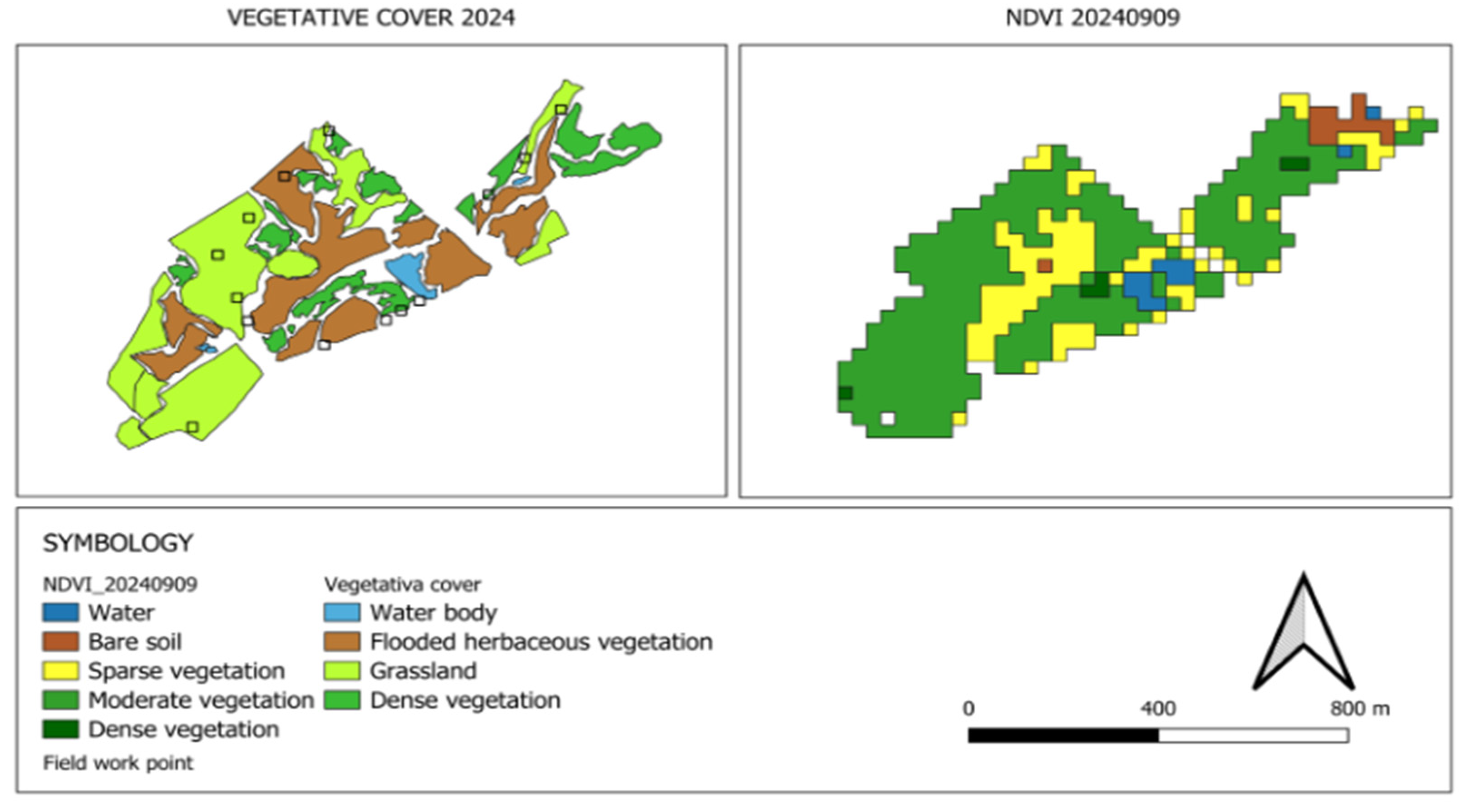
Validation of the vegetation cover maps through field observations (April 2024) showed a consistent correspondence with vegetation index values (NDVI; Figure 5). A clear spectral gradient was identified: high NDVI values (>0.6) corresponded to dense vegetation areas, intermediate values (0.2–0.4) were associated with grasslands and herbaceous cover, while low or negative values (<0.1) coincided with water bodies.

During in situ verification, wetland indicator species such as Schoenoplectus californicus and Typha angustifolia were documented, along with invasive taxa such as Ulex europaeus. Characteristic wetland birds were also recorded, including the Tropical Kingbird (Tyrannus melancholicus) and Vermilion Cardinal (Pyrocephalus rubinus). These observations provided ecological validation of the assigned spectral classes.

However, widespread anthropogenic pressures were also observed, including landfills, drainage systems, and extensive livestock grazing, which explain the atypically low NDVI values recorded along wetland edges and buffer zones. Collectively, these results confirm the robustness of the automated spectral classification and quantitatively complement the satellite analysis with direct botanical, zoological, and geospatial evidence, consolidating the foundation for subsequent predictive modeling.

3.3. Spectral Correlation Matrix Between Moisture and Vegetation Indices

The correlation matrix (

Table 4. Correlation matrix of spectral indices.

NDVI	NDWI	NDMI	MNDWI
1.000000	−0.992192	0.290679	−0.573456

Source: Authors’ elaboration.

) shows a very strong negative relationship between NDVI and NDWI (−0.99), a moderate negative correlation between NDVI and MNDWI (−0.57), and a low positive correlation between NDVI and NDMI (0.29). This indicates that areas with higher vegetation density tend to have lower surface moisture. Although the NDMI correlation is low, it was retained in the model because it provides complementary information about canopy and soil, which is useful for algorithms such as Random Forest that capture non-linear interactions.

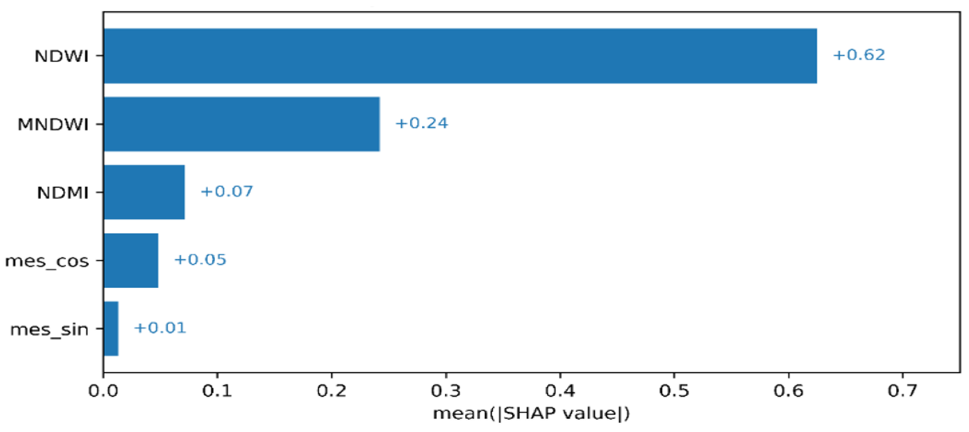
These results are complemented by the SHAP technique (Figure 6), which identified NDWI and MNDWI as the variables with the highest influence on predictions, followed by NDMI. Seasonal variables (month_sin and month_cos) showed a smaller but non-negligible contribution, indicating that temporal seasonality also partially affects vegetation spectral response, albeit to a lesser extent.

3.4. Multitemporal Analysis of NDVI (2013–2032)

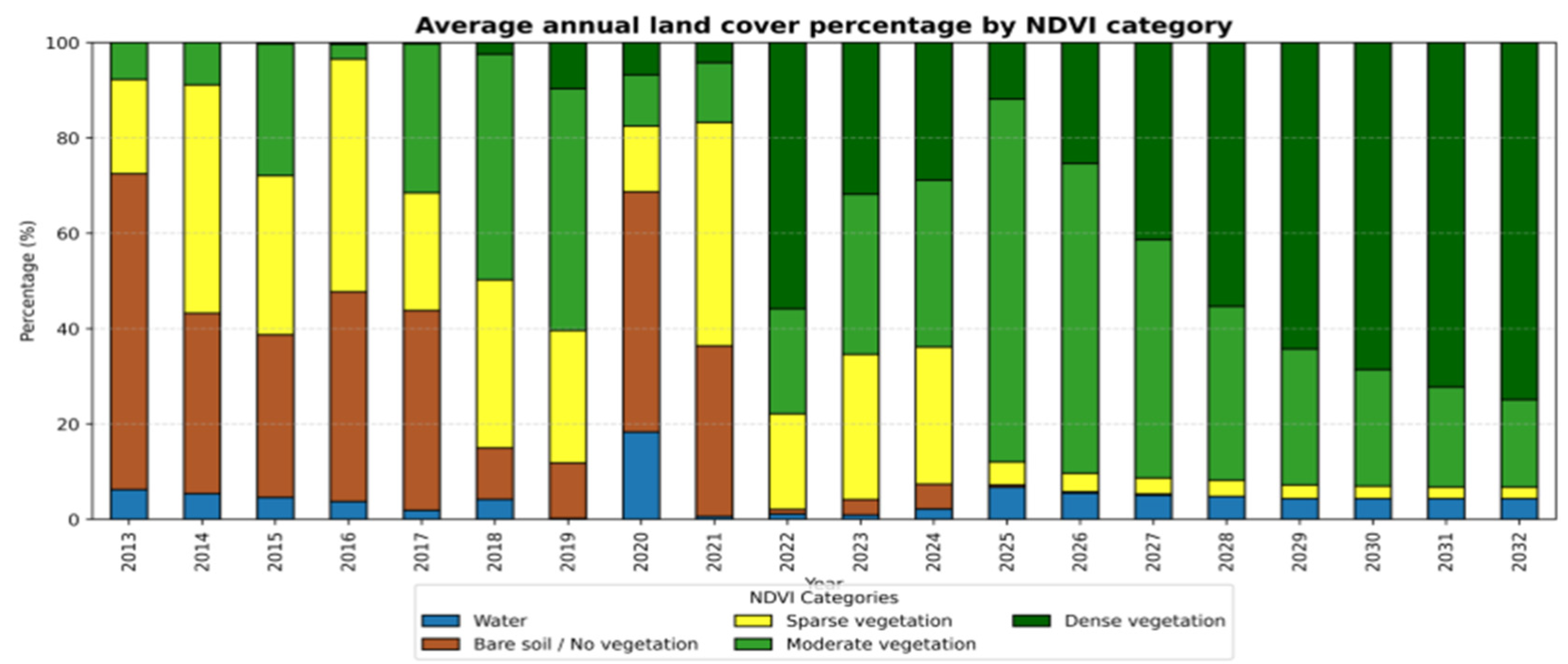
Figure 7 illustrates the temporal evolution of vegetation cover in the Capellanía wetland between 2013 and 2032. Initially, bare soil and sparse vegetation dominate, with localized water presence. From 2021 onwards, a progressive transition is observed, characterized by an increase in moderate vegetation, which exceeds 50% of the area during several periods. Starting in 2022, there is a notable increase in dense vegetation, reaching approximately 70% of the total cover by 2032.

In this context, the strong negative correlation observed between NDVI and NDWI (−0.99) does not pose a methodological issue; rather, it reflects an expected dynamic in urban wetlands. While the increase in NDVI indicates vegetation recovery, the concurrent decrease in NDWI signals a relative reduction of water-covered surfaces. This result highlights the competitive relationship between water and vegetation within the ecosystem.

The evolution of the Shannon diversity index (H′) in the Capellanía wetland between 2013 and 2032 shows marked variability in the early years (values ranging from 0.2 to 1.3), reflecting phases dominated by bare soil or sparse vegetation, alternating with periods of higher heterogeneity. From 2021 onwards, a sustained increase in structural diversity is observed, associated with the expansion of moderate vegetation, reaching values between 0.8 and 1.0.

In the projected period (2025–2032), the index tends to stabilize, although with a slight decline toward 2032, indicating the consolidation of moderate and dense vegetation cover, but with a reduced relative balance among categories. These results suggest a process of partial wetland recovery, in which vegetation cover strengthens while structural diversity gradually declines (Figure 8).

The calculation of the Compound Annual Growth Rate (CAGR) between 2013 and 2032 (

Table 5. NDVI class area (ha). Note: NA indicates that no dense vegetation was present in 2013.

Class	Percentages (%)
Water	−1.91
Bare soil/non-vegetated	−100
Sparse vegetation	−13.68
Moderate vegetation	0.91
Dense vegetation	NA

) reflects a transition from degraded covers toward increased vegetation presence. There is a sustained decrease in water and bare soil, while moderate vegetation shows a slight but consistent growth. The most notable case is dense vegetation, whose compound growth rate is infinite because it starts from zero in 2013 and consolidates by 2032. These figures confirm a reduction of degraded areas (bare soil and sparse vegetation) and a significant increase in moderate and dense vegetation.

3.5. Multitemporal NDVI Mapping (2013–2032)

Figure 9 shows the spatial distribution of vegetation classes at different dates and projections for 2025 and 2032. Each map is classified into four categories: bare soil/non-vegetated (brown), sparse vegetation (yellow), moderate vegetation (light green), and dense vegetation (dark green).

2013–2019: Dominance of bare soil and sparse vegetation, especially in the northern and eastern sectors of the wetland, with small patches of dense vegetation concentrated in the southern sector.

2020: Critical scenario characterized by strong internal fragmentation, an increase in water bodies, and a reduction in vegetation cover.

2022–2024: Transition phase with a decrease in degraded areas and an increase in moderate and dense vegetation, particularly toward the central and southwestern sectors.

2025–2032 (projections): Predominance of moderate and dense vegetation, with almost complete disappearance of degraded categories, reflecting ecological recovery and consolidation of the ecosystem.

This spatial sequence supports the numerical results and Shannon index trends, showing that the wetland is moving toward higher vegetation cover, although with progressively greater structural homogeneity by 2032.

The multitemporal mapping supports the numerical results shown in Table 4 and the NDVI graphs, illustrating how the wetland is trending toward higher vegetation cover and diversity by 2032.

3.6. Urban Simulation Scenarios (With and Without ALO)

Scenarios II and III were analyzed using cellular automata (MOLUSCE), and the results are described below:

Scenario II (with ALO): Non-urbanized areas decrease from 705.6 ha (2013) to 356.85 ha (2025, −33.8%), while urbanized areas increase from 324.09 ha to 672.30 ha (+33.8%) (

Table 6. Statistics by Class with the ALO Project (Planned Road) Scenario II.

Land Use Transition Patterns	Area 2013 (ha)	Area 2025 (ha)	∆	2013 (%)	2025 (%)	∆ (%)
0 (Unbuilt Land)	705.6	356.85	34.6	34.67	34.67	−33.83
1 (Developed Land)	324.09	672.30	63.33	65.32	65.32	33.83

and

Table 7. Transition Matrix with the ALO Project (Scenario II).

	0	1
0	0.58595	0.41404
1	0.29060	0.70931

0 = Unbuilt Land; 1 = Developed Land.

).

The transition matrix for Scenario II with the ALO project shows a land-use change dynamic where unbuilt land (State 0) has a 41.4% probability of being developed in the next period, reflecting high urbanization pressure. Conversely, already developed land (State 1) has an unusually high probability (29.1%) of reverting to unbuilt status, suggesting notable instability or reversibility in the development process under the modeled conditions.

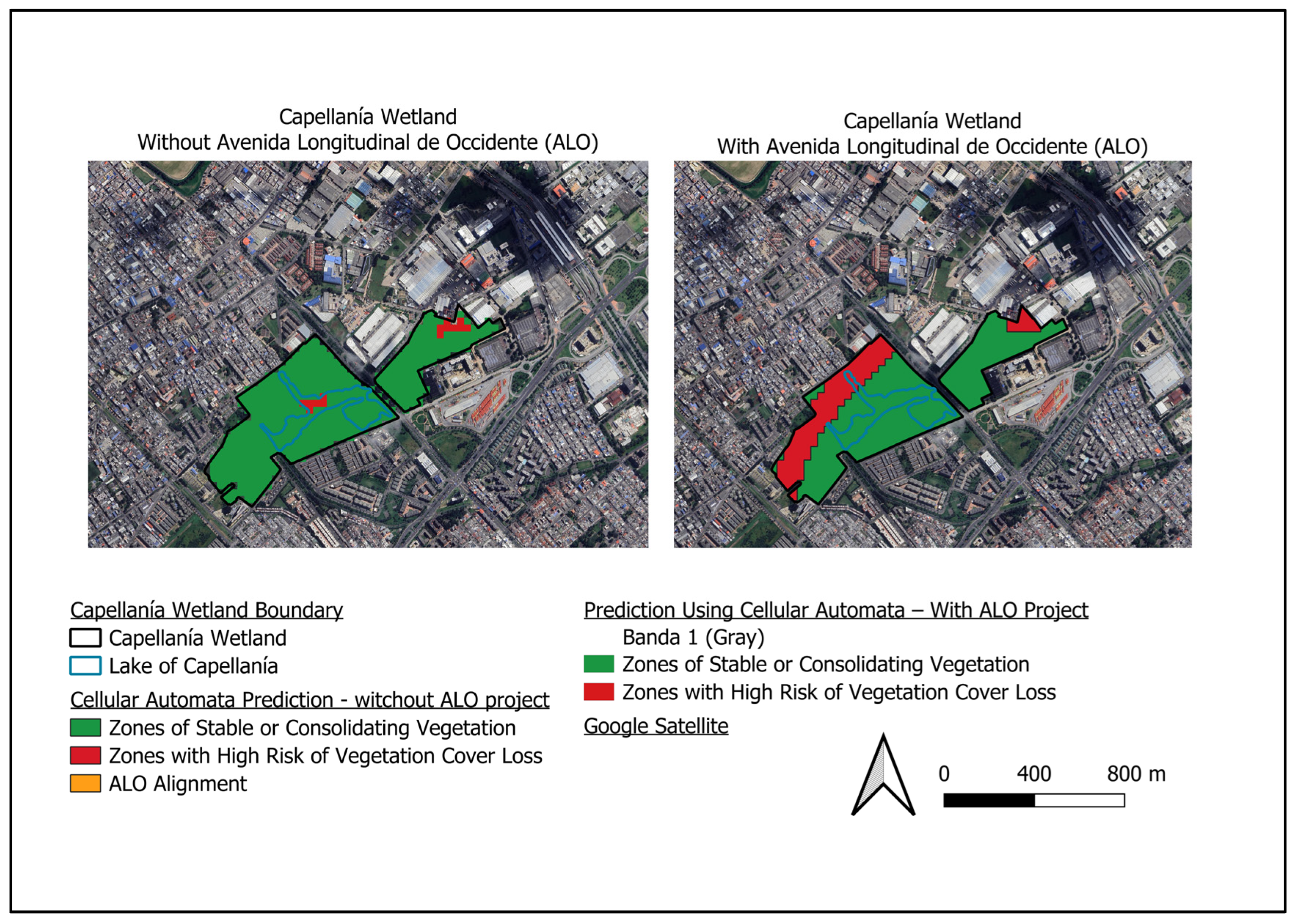
Figure 10 shows comparative results for the two projected scenarios in 2032 using the MOLUSCE cellular automata model. In the scenario without the ALO (left), large green areas correspond to stable or consolidating vegetation, with smaller red areas indicating high risk of vegetation loss. In contrast, the scenario with the ALO (right) shows a notable increase in red areas, particularly in the northeastern sector, reflecting a significant reduction in stable vegetation cover.

These results confirm that the ALO acts as a catalyst for urbanization processes, exerting greater pressure on wetland vegetation and increasing the risk of loss in adjacent areas. These findings highlight the urgent need to implement mitigation and restoration measures should the road project be executed.

The comparison between the spectral NDVI projection for 2032 and the cellular automata simulation based on NDBI, including the ALO route (Figure 10), shows strong spatial convergence in identifying areas at risk of ecological degradation. Both models highlight the northeastern sector of the wetland as critical, characterized by high NDBI and low NDVI values, indicating a direct relationship between urban intensification and vegetation loss.

Although the methodological approaches differ—NDVI projections via linear regression and Random Forest do not explicitly account for the ALO, while the cellular automata model incorporates it as a spatial variable—both models consistently indicate urban expansion as the main driver of ecological deterioration. This convergence reinforces the validity of the results and underscores the value of NDBI as an early indicator of anthropogenic pressure, particularly when integrated with vegetation indices in vulnerable urban wetlands.

4. Discussion

Machine learning-based approaches have become essential tools for wetland analysis. This study implements a methodology combining the Random Forest algorithm and Markov chains for vegetation cover analysis, complemented by cellular automata (via the MOLUSCE module) for prospective spatial simulation. The analysis relies on the calculation of vegetation, moisture, and urbanization spectral indices, selected for their demonstrated effectiveness in managing high-dimensional datasets and robustness in discriminating spectrally similar classes [50].

The relevance of these methods is supported by applications in cities facing analogous pressures, such as Barranquilla, Pakistan, Lima, and Concepción, where they proved effective in quantifying wetland degradation driven by urban expansion a [5,10,14].

It is important to note that this study was conducted exclusively for the urban Capellanía wetland in Bogotá, so its findings reflect the specific biophysical, climatic, and anthropogenic conditions of this ecosystem. While the proposed approach (spectral indices, Random Forest, MOLUSCE) proved effective in modeling vegetation dynamics and urban expansion, generalization to other wetland types, such as coastal, alpine, or rural wetlands, requires additional validation that considers the peculiarities of each environment and necessitates fieldwork [25]. Wetland classification from remote sensing data is often challenging due to seasonal vegetation dynamics [29].

Additionally, the MOLUSCE model, based on cellular automata and historical data, does not incorporate external variables such as policy decisions or socioeconomic changes; therefore, its projections should be interpreted with caution. This limitation aligns with findings from arid wetlands, such as those in Xinjiang, China, where Random Forest achieved high accuracy (99%, Kappa = 0.92) but exhibited constraints in transferring the model to other scenarios [38].

4.1. Analysis of Wetland Vulnerability Metrics

The Random Forest model for the Capellanía wetland exhibited outstanding performance, with a coefficient of determination (R²) of 0.991, a root mean square error (RMSE) of 0.0214, and a mean absolute error (MAE) of 0.0127. These results demonstrate the model’s high predictive capacity and the close agreement between estimates and observed values, providing rigorous quantitative validation for assessing wetland vulnerability, consistent with studies conducted in the Sindh province [13]. Recent research confirms that Random Forest is highly accurate across diverse contexts, including marshes and coastal wetlands, due to the integration of multiple spectral indices [43,48].

Urban areas adjacent to wetlands were validated using the cellular automata algorithm, yielding a moderate Kappa coefficient of 0.640. This is consistent with studies modeling Lake Baringo (Kenya), where Kappa values above 0.45 were reported. Cellular automata provide higher sampling efficiency and capture complex interactions between urban growth drivers and wetland dynamics [3]. These results support the ability of cellular automata to model spatially complex interactions between urban growth drivers and wetland dynamics.

4.2. Comparison of Machine Learning and Simulation Models in Land-Use Change

Combining Random Forest and cellular automata enriched the analysis of territorial dynamics. NDVI-based vegetation cover projections accurately identified areas directly influencing the wetland, confirming the utility of Random Forest in urban environments. Studies in Sindh highlighted its robustness in vulnerable ecosystems [13]. Other studies have also demonstrated Random Forest’s ability to integrate spectral indices (NDVI, NDWI, NDBI) and improve predictions in urban and wetland contexts [51].

Concurrently, MOLUSCE successfully captured neighborhood effects and local spatial dynamics, demonstrating its potential for evaluating urban growth scenarios. Simulations for the Capellanía wetland, including the projection of the (ALO), indicate that this infrastructure could threaten ecological integrity, increasing pressure on vegetation. This finding aligns with studies such as “Urban Wetland Trends in Three Latin American Cities” (Rojas et al., 2020), which identify urban expansion as a critical threat to metropolitan wetlands [5]. Additionally, Cuéllar & Pérez (2023) [19] applied a hybrid model (Markov-ANN-FLUS) to 15 urban wetlands in Bogotá, projecting a nearly 25% reduction by 2034 and highlighting Capellanía as one of the most affected ecosystems by urbanization. These findings support our results and emphasize the need to consider road infrastructure scenarios like the ALO in urban wetland planning and conservation. Similar predictive approaches have been successfully applied at Lake Baringo using neural networks and cellular automata [3].

Overall, these discussions demonstrate that the results obtained for the Capellanía wetland are consistent with global and regional trends. Despite significant surrounding urban pressure, there is a clear trend toward vegetation cover recovery and progressive consolidation of the wetland core, underscoring the relevance of implementing comprehensive planning and ecological restoration measures. Simultaneously, urban simulation projections confirm that infrastructure projects, such as the ALO, can dramatically accelerate vegetation loss in adjacent areas. These conclusions, supported by both current remote sensing data and recent scientific literature, provide a solid foundation for management, conservation, and decision-making in urban wetlands facing similar ecological characteristics and anthropogenic pressures.

4.3. Structural Diversity and Ecological Resilience (Shannon Index Analysis)

Shannon index values correspond with observations in the Capellanía Wetland Environmental Management Plan (2008) [20], which noted a loss of structural diversity due to water body drying and the predominance of degraded covers [1]. The marked variability observed between 2013 and 2020, with index declines approaching zero, reflects this ecosystem fragility and the temporal dominance of categories such as bare soil or sparse vegetation.

From 2021 onwards, the increase in moderate vegetation and the consequent recovery of diversity aligns with the 2023 Management Report of the RDH Capellanía, highlighting improvements in water quality, vegetation restoration processes, and strengthened community monitoring [2,19]. However, index stabilization around intermediate values (0.8–1.0) toward 2032 indicates that, although vegetation cover recovers, structural diversity tends to decrease due to the dominance of moderate and dense vegetation.

This finding suggests that the ecosystem is moving toward a more homogeneous state, which, while indicative of recovery, limits long-term ecological resilience. Therefore, restoration actions should aim to preserve cover heterogeneity, ensuring not only increased vegetation cover but also structural diversity that supports the ecological stability of the wetland.

5. Conclusions

The results demonstrate a clear transition in vegetation cover in the Capellanía Wetland between 2013 and 2032. Degraded classes (bare soil and sparse vegetation) decreased from over 80% to less than 10%, while moderate and dense vegetation increased steadily to exceed 90% by the end of the period. Water cover remained low but stable. These changes reflect a progressive recovery process and consolidation of vegetation, in contrast with the loss trends observed in other Latin American urban wetlands, such as the Ciénaga de Mallorquín.

Methodologically, this study demonstrates the value of integrating a multitemporal Random Forest model (R² = 0.991; RMSE = 0.0214; MAE = 0.0127) with spatial simulations based on cellular automata in MOLUSCE. This approach proved effective in anticipating ecological trajectories, identifying critical areas, and guiding targeted restoration strategies. The strong negative correlation between NDVI and NDWI (–0.99), along with vegetation consolidation in the core and potential loss along the northeastern edges, underscores the need for specific interventions to maintain ecological connectivity.

Urbanization scenario analysis confirms that the construction of the (ALO) would act as a catalyst for urban expansion, drastically reducing non-urbanized areas and increasing pressure on vegetation. This finding provides critical input for strategic environmental assessments and highlights the necessity of integrating spatial modeling into road and territorial planning in Bogotá.

Overall, this study provides quantitative, spatial, and prospective evidence to inform conservation policies and sustainable urban planning. The results advocate for preventive, integrated, and data-driven approaches to ensure the protection of strategic wetlands like Capellanía, which perform essential ecological functions within the urban matrix.

Finally, a limitation of this study is the absence of integrated climatic and socioeconomic variables due to resolution and data quality constraints, presenting an opportunity for model expansion in future research. It is also recommended to explore participatory management scenarios and incorporate in situ data to strengthen decision-making and promote more effective environmental governance in urban wetlands across Latin America.

References

1. González Angarita, G.; Henríquez, C.; Peña Angulo, D.; Castro Álvarez, D.; Forero Buitrago, G. Geomatic Analysis Techniques in the Loss of Urban. Wetlands in Bogotá. What Role Do Ilegal Settlements Play? Rev. De Geogr. De Norte Gd. 2022, 81, 207–233. [Google Scholar] [CrossRef]
2. IPBES. Global Assessment Report on Biodiversity and Ecosystem Services; IPBES: Bonn, Germany, 2019; Available online: https://ipbes.net/ (accessed on 14 April 2025).
3. Kimtai, D.J.; Makokha, G.O.; Sichangi, A.W. Modeling of Water Level Trends and Characterizing Potential Influencing Factors in Lake Baringo, Kenya. Discov. Water 2024, 4, 55. [Google Scholar] [CrossRef]
4. Ballut-Dajud, G.A.; Herazo, L.C.S.; Fernández-Lambert, G.; Marín-Muñiz, J.L.; Méndez, M.C.L.; Betanzo-Torres, E.A. Factors Affecting Wetland Loss: A Review. Land 2022, 11, 434. [Google Scholar] [CrossRef]
5. Rojas, C.; Aldana-Domínguez, J.; Munizaga, J.; Moschella, P.; Martínez, C.; Stamm, C. Urban Wetland Trends in Three Latin American Cities during Recent Decades (2002–2019): Concon (Chile), Barranquilla (Colombia) and Lima (Perú). Wetl. Sci. Pract. 2020, 37, 283–293. [Google Scholar] [CrossRef]
6. Ariza, A.; Garcia, S.; Rojas, S.; Ramírez, M. Development of a Satellite Image Correction Model for Floods: (CAIN—Atmospheric Correction and Flood Indices). Technical Report; Instituto Geográfico Agustín Codazzi (IGAC): Bogotá, Colombia, 2013; Available online: https://un-spider.org/sites/default/files/ModeloCAIN.pdf (accessed on 15 March 2025).
7. García, C. PM Particulate Matter Concentration as a Function of Humidity and Atmospheric Reflectance Using Landsat-8 Images in Metropolitan Lima, 2015–2016. Rev. Cient. Pakamuros 2023, 6, v77ptx88. [Google Scholar] [CrossRef]
8. Lv, J.; Jiang, W.; Wang, W.; Wu, Z.; Liu, Y.; Wang, X.; Li, Z. Wetland Loss Identification and Evaluation Based on Landscape and Remote Sensing Indices in Xiong’an New Area. Remote Sens. 2019, 11, 2834. [Google Scholar] [CrossRef]
9. Sabogal Vélez, C.L.; Pedroza Toro, L.M.; González Angarita, G.P. Vegetation Analysis Using Spectral Indices and Its Relevance for Identifying Water Bodies in the Torca Guaymaral Wetland, Bogotá, Colombia. Av. Investig. Ing. 2023, 20, 10708. [Google Scholar] [CrossRef]
10. Olmedo, M.T.C.; Pontius, R.G.; Paegelow, M.; Mas, J.-F. Comparison of Simulation Models in Terms of Quantity and Allocation of Land Change. Environ. Model. Softw. 2015, 69, 214–221. [Google Scholar] [CrossRef]
11. Zhang, J.; Liu, X.; Qin, Y.; Fan, Y.; Cheng, S. Wetlands Mapping and Monitoring with Long-Term Time Series Satellite Data Based on Google Earth Engine, Random Forest, and Feature Optimization: A Case Study in Gansu Province, China. Land 2024, 13, 1527. [Google Scholar] [CrossRef]
12. Jafarzadeh, H.; Mahdianpari, M.; Gill, E.W.; Brisco, B.; Mohammadimanesh, F. Remote Sensing and Machine Learning Tools to Support Wetland Monitoring: A Meta-Analysis of Three Decades of Research. Remote Sens 2022, 14, 6104. [Google Scholar] [CrossRef]
13. Aslam, R.W.; Shu, H.; Naz, I.; Quddoos, A.; Yaseen, A.; Gulshad, K.; Alarifi, S.S. Machine Learning-Based Wetland Vulnerability Assessment in the Sindh Province Ramsar Site Using Remote Sensing Data. Remote Sens. 2024, 16, 928. [Google Scholar] [CrossRef]
14. De Los Reyes, J.E.M.; Castro, J.F.H.; Páez, M.E.M. Identification of Wetland Complexes Using Satellite Images and Machine Learning, Piamonte Municipality, Cauca (Colombia). Rev. Noved. Colomb. 2024, 19, 30–45. [Google Scholar] [CrossRef]
15. González, G.P. The Impact of Urban Dynamics on the Wetlands of Bogotá (Colombia). Ph.D. Thesis, Universidad de Zaragoza, Zaragoza, España, 2018. Available online: https://zaguan.unizar.es/record/98389/files/%20TESIS-2021-010.pdf (accessed on 10 October 2024).
16. Belgiu, M.; Drăguţ, L. Dragut. Random forest in remote sensing: A review of applications and future directions. ISPRS J. Photogramm. Remote Sens. 2016, 114, 24–31. [Google Scholar] [CrossRef]
17. Moreno, V.; García, J.F.; Villalba, J.C. Descripción General de los Humedales de Bogotá, D.C. Sociedad Geográfica de Colombia; Academia de Ciencias Geográficas; Bogotá, Colombia, diciembre de 2002. Available online: https://www.researchgate.net/publication/338897341_Descripcion_General_de_los_humedales_de_Bogota_DC (accessed on 10 October 2024).
18. Cruz Solano, D.P.; Motta Morales, J.E. Estimation of Area Loss in the Bogotá Wetlands in the Last Five Decades Due to Construction and its Respective Effects. Trabajo de Grado, Universidad Distrital Francisco José de Caldas, Bogotá D.C., Colombia. 2012. Available online: https://repository.udistrital.edu.co/items/c7198b2d-b095-4708-8e57-ee39d2fd19da (accessed on 10 October 2024).
19. Cuellar, Y.; Perez, L. Multitemporal modeling and simulation of the complex dynamics in urban wetlands: The case of Bogota, Colombia. Sci. Rep. 2023, 13, 9374. [Google Scholar] [CrossRef]
20. Empresa de Acueducto de Bogotá. Environmental Management Plan Capellanía Wetland. 2008. Available online: https://oab.ambientebogota.gov.co/?post_type=dlm_download&p=15032 (accessed on 15 February 2025).
21. Alcaldía Mayor de Bogotá. General Characterization of Risk Scenarios; Alcaldía Mayor de Bogotá: Bogotá, Colombia, 2018. [Google Scholar]
22. Fennessy, M.S.; Jacobs, A.D.; Kentula, M.E. Review of Rapid Methods for Assessing Wetland Condition; US Environmental Protection Agency: Washington, DC, USA, 2004.
23. Baeza, S.; Paruelo, J.M. Land Use/Land Cover Change (2000–2014) in the Rio de la Plata Grasslands: An Analysis Based on MODIS NDVI Time Series. Remote Sens. 2020, 12, 381. [Google Scholar] [CrossRef]
24. Mahdavi, S.; Salehi, B.; Granger, J.; Amani, M.; Brisco, B.; Huang, W. Remote sensing for wetland classification: A comprehensive review. Giscience Remote Sens. 2017, 55, 623–658. [Google Scholar] [CrossRef]
25. Zhu, G.; Zhang, Y.; Shen, C.; Luo, X.; Yao, X.; Chen, G.; Xie, T.; Dong, Z. Mapping Vegetation-Covered Water Areas Using Sentinel-2 and RadarSat-2 Data: A Case Study of the Caohai Wetland in Guizhou Province. Water 2025, 17, 729. [Google Scholar] [CrossRef]
26. Guo, M.; Li, J.; Sheng, C.; Xu, J.; Wu, L. A Review of Wetland Remote Sensing. Sensors 2017, 17, 777. [Google Scholar] [CrossRef]
27. European Environment Agency. Corine land Cover; European Environment Agency: Copenhagen, Denmark, 1995. [Google Scholar]
28. Castro, E.M.C. Multitemporal Analysis of Deforestation Indices in the Yambrasbamba District, Bongará, Amazonas, Peru. Revista Científica UNTRM Ciencias Naturales e Ingeniería 2021, 5, 20–28. [Google Scholar] [CrossRef]
29. Duarte, L.; Queirós, C.; Teodoro, A.C. Comparative Analysis of Four QGIS Plugins for Web Map Creation. La Granja Rev. De Cienc. De La Vida 2021, 34, 8–26. [Google Scholar] [CrossRef]
30. Melnyk, O.; Brunn, A. Analysis of Spectral Index Interrelationships for Vegetation Condition Assessment on the Example of Wetlands in Volyn Polissya, Ukraine. Earth 2025, 6, 28. [Google Scholar] [CrossRef]
31. De La Iglesia Martinez, A.; Labib, S.M. Demystifying normalized difference vegetation index (NDVI) for greenness exposure assessments and policy interventions in urban greening. Environ. Res. 2023, 220, 115155. [Google Scholar] [CrossRef] [PubMed]
32. Zhang, L.; Zeng, Y.; Zhuang, R.; Szabó, B.; Manfreda, S.; Han, Q.; Su, Z. In Situ Observation-Constrained Global Surface Soil Moisture Using Random Forest Model. Remote Sens. 2021, 13, 4893. [Google Scholar] [CrossRef]
33. McFeeters, S.K. The use of the Normalized Difference Water Index (NDWI) in the delineation of open water features. Int. J. Remote Sens. 1996, 17, 1425–1432. [Google Scholar] [CrossRef]
34. Kennedy, R.E.; Yang, Z.; Cohen, W.B. Detecting trends in forest disturbance and recovery using yearly Landsat time series: 1. LandTrendr—Temporal segmentation algorithms. Remote Sens. Environ. 2010, 114, 2897–2910. [Google Scholar] [CrossRef]
35. Wilson, N.R.; Norman, L.M. Analysis of vegetation recovery surrounding a restored wetland using the normalized difference infrared index (NDII) and normalized difference vegetation index (NDVI). Int. J. Remote Sens. 2018, 39, 3243–3274. [Google Scholar] [CrossRef]
36. Muhammad, R.; Zhang, W.; Abbas, Z.; Guo, F.; Gwiazdzinski, L. Spatiotemporal Change Analysis and Prediction of Future Land Use and Land Cover Changes Using QGIS MOLUSCE Plugin and Remote Sensing Big Data: A Case Study of Linyi, China. Land 2022, 11, 419. [Google Scholar] [CrossRef]
37. Fontana, A.G.; Nascimento, V.F.; Ometto, J.P.; do Amaral, F.H.F. Analysis of past and future urban growth on a regional scale using remote sensing and machine learning. Front. Remote Sens. 2023, 4, 1123254. [Google Scholar] [CrossRef]
38. Alipbeki, O.; Alipbekova, C.; Mussaif, G.; Grossul, P.; Zhenshan, D.; Muzyka, O.; Turekeldiyeva, R.; Yelubayev, D.; Rakhimov, D.; Kupidura, P.; et al. Analysis and Prediction of Land Use/Land Cover Changes in Korgalzhyn District, Kazakhstan. Agronomy 2024, 14, 268. [Google Scholar] [CrossRef]
39. Gündüz, H.I. Land-Use Land-Cover Dynamics and Future Projections Using GEE, ML, and QGIS-MOLUSCE: A Case Study in Manisa. Sustainability 2025, 17, 1363. [Google Scholar] [CrossRef]
40. Seto, K.C.; Güneralp, B.; Hutyra, L.R. Global forecasts of urban expansion to 2030 and direct impacts on biodiversity and carbon pools. Proc. Natl. Acad. Sci. USA 2012, 109, 16083–16088. [Google Scholar] [CrossRef]
41. Wang, H.; Yang, C.; Sun, Y.; Liu, H.; Liu, Y.; Xing, H. A New Method for Evaluating the Coordinated Relationship Between Vegetation Greenness and Urbanization. Sci. Rep. 2025, 15, 6003. [Google Scholar] [CrossRef]
42. Tan, X.; Shan, Y.; Wang, X.; Liu, R.; Yao, Y. Comparison of the predictive ability of spectral indices for commonly used species diversity indices and Hill numbers in wetlands. Ecol. Indic. 2022, 142, 109233. [Google Scholar] [CrossRef]
43. Verburg, P.H.; Alexander, P.; Evans, T.; Magliocca, N.R.; Malek, Z.; DA Rounsevell, M.; van Vliet, J. Beyond land cover change: Towards a new generation of land use models. Curr. Opin. Environ. Sustain. 2019, 38, 77–85. [Google Scholar] [CrossRef]
44. Rounsevell, M.D.A.; Arneth, A.; Alexander, P.; Brown, D.G.; de Noblet-Ducoudré, N.; Ellis, E.; Finnigan, J.; Galvin, K.; Grigg, N.; Harman, I.; et al. Towards decision-based global land use models for improved understanding of the Earth system. Earth Syst. Dyn. 2014, 5, 117–137. [Google Scholar] [CrossRef]
45. Jaeger, J.A.; Bertiller, R.; Schwick, C.; Kienast, F. Suitability criteria for measures of urban sprawl. Ecol. Indic. 2010, 10, 397–406. [Google Scholar] [CrossRef]
46. Santé, I.; García, A.M.; Miranda, D.; Crecente, R. Cellular automata models for the simulation of real-world urban processes: A review and analysis. Landsc. Urban Plan. 2010, 96, 108–122. [Google Scholar] [CrossRef]
47. Maxwell, A.E.; Warner, T.A.; Fang, F. Implementation of machine-learning classification in remote sensing: An applied review. Int. J. Remote Sens. 2018, 39, 2784–2817. [Google Scholar] [CrossRef]
48. Suir, G.M.; Jackson, S.; Saltus, C.; Reif, M. Multi-Temporal Trend Analysis of Coastal Vegetation Using Metrics Derived from Hyperspectral and LiDAR Data. Remote Sens. 2023, 15, 2098. [Google Scholar] [CrossRef]
49. Tian, S.; Zhang, X.; Tian, J.; Sun, Q. Random Forest Classification of Wetland Landcovers from Multi-Sensor Data in the Arid Region of Xinjiang, China. Remote Sens. 2016, 8, 954. [Google Scholar] [CrossRef]
50. Windle, A.E.; Staver, L.W.; Elmore, A.J.; Scherer, S.; Keller, S.; Malmgren, B.; Silsbe, G.M. Multi-temporal high-resolution marsh vegetation mapping using unoccupied aircraft system remote sensing and machine learning. Front. Remote Sens. 2023, 4, 1140999. [Google Scholar] [CrossRef]
51. Wang, M.; Mao, D.; Wang, Y.; Song, K.; Yan, H.; Jia, M.; Wang, Z. Annual Wetland Mapping in Metropolis byTemporal Sample Migration and Random Forest Classification with Time Series Landsat Data and Google Earth Engine. Remote Sens. 2022, 14, 3191. [Google Scholar] [CrossRef]
Figure 1. Methodological workflow for the multitemporal analysis of spectral indices and predictive modeling of NDVI and NDBI (2013–2032) in the Capellanía Wetland, integrating QGIS 3.34, Python v.3.11.7, and MOLUSCE v 4.2.1 cellular automata.
Sustainability 17 08462 g001
Figure 2. Study area: Location of the Capellanía wetland. Multi-scale maps from Colombia to the UPZ level, showing the wetland boundary, lake, Fontibón locality, and the projected Avenida Longitudinal de Occidente (ALO) over satellite imagery.
Sustainability 17 08462 g002
Figure 3. Field survey and identification of the main vegetation covers in the Capellanía wetland.
Sustainability 17 08462 g003
Figure 4. Current NDVI and NDBI of the Capellanía wetland. Vegetation cover classification into four categories and areas with probability of vegetation loss, derived from NDVI and NDBI indices on satellite imagery.
Sustainability 17 08462 g004
Figure 5. Comparison between NDVI indices and Vegetation Cover Map.
Sustainability 17 08462 g005
Figure 6. Relative contribution of each predictor according to SHAP analysis.
Sustainability 17 08462 g006
Figure 7. Percentage of area by NDVI category (2013–2032) in the Capellanía wetland.
Sustainability 17 08462 g007
Figure 8. Shannon diversity index (H′) of vegetation cover in the Capellanía Wetland (2013–2032), showing phases of heterogeneity, homogenization, and partial recovery.
Sustainability 17 08462 g008
Figure 9. Spatial evolution and projection of vegetation cover in the Capellanía Wetland (2013–2032), classified into four NDVI categories.
Sustainability 17 08462 g009
Figure 10. Predicted vegetation cover change in the Capellanía Wetland for 2032: Classification into stable/consolidating vegetation zones and zones at high risk of vegetation loss, obtained using cellular automata applied to satellite imagery.
Sustainability 17 08462 g010