Constructing Real-Time Meteorological Forecast Method of Short-Term Cyanobacteria Bloom Area Index Changes in the Lake Taihu

Abstract

The dynamics of cyanobacteria bloom in Lake Taihu, China, are subject to rapid fluctuations under the influence of various factors, with meteorological conditions being particularly influential. In this study, monitoring data on the surface area of cyanobacteria bloom in Lake Taihu and observational data from automatic meteorological stations around Lake Taihu from 2016 to 2022 were utilized. Meteorological sub-indices were constructed based on the probability density distributions of meteorological factors in different areas of cyanobacterial bloom. A stacked ensemble model utilizing various machine learning algorithms was developed. This model was designed to forecast the cyanobacterial bloom area index in Lake Taihu based on meteorological data. This model has been deployed with real-time gridded forecasts from the China Meteorological Administration (CMA) to predict changes in the cyanobacteria bloom area index in Lake Taihu over the next 7 days. The results demonstrate that utilizing meteorological sub-indices, rather than traditional meteorological elements, provides a more effective reflection of changes in cyanobacteria bloom area. Key meteorological sub-indices were identified through recursive feature elimination, with wind speed variance and wind direction variance highlighted as especially important factors. The real-time forecasting system operated over a 2.5-year period (2023 to July 2025). Results demonstrate that for cyanobacteria bloom areas exceeding 100 km², the 1-day lead-time forecast hit rate exceeded 72%, and the 3-day forecast hit rate remained above 65%. These findings significantly enhance forecasting capability for cyanobacterial blooms in Lake Taihu, offering critical support for sustainable water management practices in one of China’s most important freshwater systems.

1. Introduction

The eutrophication problem constitutes one of the critical environmental issues confronting lakes, with the frequent cyanobacterial blooms being a significant manifestation of this ecological degradation in aquatic systems [1,2]. Influenced by factors such as climate change and eutrophication, the frequency, intensity, and duration of cyanobacterial bloom outbreaks in many global aquatic ecosystems have shown an increasing trend [3]. Analysis of over 100 lakes in North America and Europe indicates that since 1945, approximately 60% of these lakes have experienced an accelerating growth rate of cyanobacteria [4]. In the USA’s Lake Erie, cyanobacterial blooms had reappeared by the mid-1990s and have been on the rise since, with the bloom area reaching 5000 square kilometers in 2011 [5]. Similarly, Lake Taihu in China has frequently experienced cyanobacterial blooms since the 1980s, with the bloom coverage reaching 1217 square kilometers in 2017 [6]. Cyanobacterial blooms are also expanding in estuarine and marine ecosystems. Dai et al. [7] found that since the beginning of the 21st century, the area and frequency of coastal phytoplankton blooms have been increasing globally.

Cyanobacterial blooms pose significant risks to water quality. These blooms increase turbidity and can smother submerged aquatic vegetation, thereby reducing light penetration. The microbial degradation of senescent blooms leads to oxygen depletion, which may induce hypoxic or anoxic conditions, resulting in the death of fish and benthic invertebrates. Additionally, cyanobacteria produce taste and odor compounds that interfere with recreational use of lakes and affect the suitability of reservoirs for drinking water [3]. For instance, in August 2014, a ‘do not drink’ advisory was issued in Toledo, OH, USA, when microcystin levels exceeded the World Health Organization (WHO) guideline value for safe drinking water, leaving over 400,000 residents without tap water for nearly 48 h [8]. Similarly, the 2007 cyanobacterial bloom crisis in Lake Taihu triggered a drinking water crisis in Wuxi City [9]. Given these impacts, forecasting and providing early warnings for cyanobacterial blooms are essential for managing water quality in lakes prone to such occurrences, such as Lake Taihu [10].

Cyanobacterial blooms occur in lakes experiencing eutrophication due to human activities that release significant amounts of nitrogen and phosphorus. These conditions are further exacerbated by favorable meteorological and hydrodynamic settings [11]. Numerous observations confirm that cyanobacterial blooms in Lake Taihu exhibit distinct spatiotemporal variations [12,13]. The inter-annual variability of these blooms is influenced by both changes in nutrient concentrations and meteorological factors [14], while daily and hourly fluctuations are predominantly driven by elements such as wind speed and temperature [15]. Changes in wind patterns play a particularly crucial role in the dynamics of bloom formation [16,17]. The predictability of meteorological and hydrodynamic elements enables the forecasting of rapid changes in cyanobacterial bloom coverage.

Researchers have developed various methods and models to forecast the dynamic variations in cyanobacterial blooms [18]. Zhang et al. [19] and Stumpf et al. [8] established annual forecasting methods for cyanobacterial bloom intensity in Lake Taihu and Lake Erie using meteorological elements and nutrient concentrations, respectively, both achieving good fitting results [8,19]. The hydrodynamic-algal biomass coupled model developed by Li et al. [18] can predict chlorophyll-a concentrations in different regions of Lake Taihu, with prediction accuracy exceeding 80% for short-term bloom forecasts. With advancements in machine learning technology, an increasing number of artificial intelligence methods have also been applied to cyanobacterial bloom forecasting [20,21]. Ni et al. [22] predicted chlorophyll-a concentration in the Lake Taihu using a deep learning model, achieving promising forecasting results. Sandubete-López et al. [23] and Fournier et al. [24] used Long Short-Term Memory (LSTM) models to predict cyanobacterial blooms, achieving over 70% accuracy for long-term forecasts in the Cuerda del Pozo reservoir, Spain. Currently, most forecasting models predict chlorophyll-a concentration or algal density at specific regions or monitoring sites, lacking research on predicting short-term changes in cyanobacterial bloom coverage. However, the surface area of blooms can be monitored using satellites, which offer the advantage of high spatial and temporal resolution. This method is widely used to assess cyanobacterial bloom intensity in lakes and reservoirs [5,25]. Changes in algal density and chlorophyll-a concentration, constrained by monitoring locations, differ significantly from changes in bloom surface area [26]. The short-term variation in bloom coverage is primarily influenced by meteorological conditions. Therefore, there is a need to evaluate meteorological forecasting methods for short-term changes in cyanobacterial bloom area to enhance predictive and early warning capabilities.

This study aims to forecast short-term changes in the surface area of cyanobacterial blooms in Lake Taihu. Meteorological sub-indices are constructed based on wind fields over Lake Taihu and other meteorological elements that influence the dynamic variations in cyanobacterial blooms. The impact of these meteorological sub-indices on the bloom area is analyzed. A stacking ensemble model based on multiple machine learning algorithms is employed to predict the Lake Taihu cyanobacterial bloom area. We conducted a real-time forecasting experiment on short-term variations in cyanobacterial bloom area over a 2.5-year period, utilizing the China Meteorological Administration’s Grid Weather Forecast products. This paper develops a meteorological forecasting model targeting the short-term variation in cyanobacterial bloom area in Lake Taihu, identifies key meteorological sub-indices influencing rapid changes in area, and provides robust support for forecasting, early warning, and effective management of cyanobacterial blooms.

2. Materials and Methods

2.1. Cyanobacterial Bloom Area Monitoring

The cyanobacterial bloom area in Lake Taihu was monitored using data from the Moderate Resolution Imaging Spectroradiometer (MODIS) onboard the Terra satellite during the period 2016 to July 2025, with a spatial resolution of 250 m. The inversion method for estimating cyanobacterial bloom coverage utilized the Normalized Difference Vegetation Index (NDVI) method (Formula (1)). Images obscured by clouds were excluded. he NDVI values of cyanobacterial blooms in Lake Taihu are affected by atmospheric conditions and the solar zenith angle, resulting in significant variations in the applicable NDVI thresholds. Therefore, the daily NDVI threshold was established by visually distinguishing between the lake surface and cyanobacterial bloom areas. The bloom-covered regions were delineated using these manually defined NDVI thresholds (−0.15 to 0.10), which align with ranges reported in previous studies [27,28]. This process yielded a total of 558 valid images. Given that the annual maximum bloom area shows significant variations, mainly influenced by factors such as winter temperature and nutrient levels [19], and daily variations in blooms are primarily driven by fluctuations in meteorological elements like wind fields and temperature [14], this study applied normalization to the Lake Taihu cyanobacterial bloom area data (Formula (2)). This approach aimed to better characterize short-term variations in cyanobacterial blooms and minimize the impact of inter-annual changes on predictive model construction. Model training and testing utilized data from 2016 to 2022, while data from 2023 to July 2025 were used for real-time validation of model forecasting results.

$$NDVI=\left(NIR-R\right)/\left(NIR+R\right)$$

(1)

$${area}_{st}={\displaystyle \frac{area}{{area}_{95}}}$$

(2)

where NIR is the near-infrared band, R is the red band, area represents the Lake Taihu cyanobacterial bloom area, ${area}_{95}$ represents the 95th percentile value of the bloom coverage within a year, and ${area}_{st}$ represents the normalized Lake Taihu cyanobacterial bloom area index for a specific day.

2.2. Meteorological Data and Processing Methods

Meteorological data were obtained from 40 automatic weather stations located within Lake Taihu and along its shores (Figure 1), operated by the China Meteorological Administration. Monitored meteorological elements included wind direction, wind speed, temperature, hourly precipitation, and humidity. Among these, the Dongshan station in Lake Taihu provided additional data on atmospheric pressure, visibility, sunshine duration, cloud cover, and evaporation, because it is a manned meteorological observation station equipped with more comprehensive instrumentation than other automatic observation stations.

The meteorological data were divided into training and testing datasets. The training dataset comprised data from 2016 to 2021 (478 samples). The testing dataset consisted of data from 2022, comprising 80 samples. Subsequent meteorological sub-index construction and model training utilized only the training dataset. To further validate the applicability of the proposed model, daily grid forecast data from the China Meteorological Administration for the period from 2023 to July 2025 were employed to forecast the Lake Taihu cyanobacterial bloom area index for the subsequent 7 days.

Qin et al. [16] demonstrated that wind-driven convergence and divergence of lake currents predominantly determine the distribution and accumulation patterns of cyanobacterial blooms. However, previous studies relying on averaged wind speed measurements from surrounding stations inadequately characterize the spatial heterogeneity of Taihu’s wind field. This study therefore employed statistical analyses including mean wind speed, mean wind direction, wind direction variance, and wind speed variance to quantify wind field variations. Variance metrics of wind direction and speed reflect spatial consistency across the lake region; higher variance indicates localized convergence/divergence or abrupt wind shifts. Such wind field perturbations can trigger bloom outbreaks or rapid dissipation. Accordingly, spatio-temporal variations in the wind field were characterized using variance metrics for wind speed and wind direction.

As most satellite observations occurred during morning and afternoon periods, wind field data from 08:00 to 14:00 local time were specifically analyzed to capture meteorological conditions preceding satellite detection windows. A total of 30 meteorological variables were derived to construct meteorological sub-indices. Computational methods are detailed in

Table 1. Calculation method of meteorological factors.

Meteorological Factor	Calculation Method	Meteorological Factor	Calculation Method
Hourly mean wind direction $(\overline{wd})$	The wind direction of the vector sum under the assumption of uniform wind speed	Wind direction, wind speed, wind direction variance, and wind speed variance from 08:00 to 14:00	based on the wind field data from 08:00 to 14:00
Hourly mean wind speed $\left(\overline{ws}\right)$	${\displaystyle \raisebox{1ex}{$\sum {ws}_i$}\!\left/ \!\raisebox{-1ex}{$n$}\right.}$	Daily mean temperature ($\overline{T}$)	Average temperature form all the stations and all the hours
Hourly wind direction variance	$\sqrt{\sum {({wd}_i-\overline{wd})}^2}$	5-day accumulated temperature (AT)	${\displaystyle \raisebox{1ex}{${\sum }_{d-4}^d{\overline{T}}_d$}\!\left/ \!\raisebox{-1ex}{$5$}\right.}$
Hourly wind speed variance	$\sqrt{\sum {({ws}_i-\overline{ws})}^2}$	5-day accumulated temperature variation (dAT)	${AT}_d-{AT}_{d-1}$
Daily mean wind speed (${\overline{ws}}_d$)	${\displaystyle \raisebox{1ex}{$\sum {\overline{ws}}_h$}\!\left/ \!\raisebox{-1ex}{$24$}\right.}$	Daily precipitation (Pre)	Average daily precipitation form all the stations
Daily wind speed variance	$\sqrt{\sum {({\overline{ws}}_h-{\overline{ws}}_d)}^2}$	Precipitation in the previous 1–3 days (${Pre}_3$)	${Pre}_{d-1}+{Pre}_{d-2}+{Pre}_{d-3}$
Daily mean wind direction (${\overline{wd}}_d$)	Daily-averaged vectors of $\overline{wd}$	Daily mean RH	Dongshan Station
Daily wind direction variance	$\sqrt{\sum {({\overline{wd}}_h-{\overline{wd}}_d)}^2}$	Daily average air pressure	Dongshan Station
Daily maximum wind speed	The maximum value of $\overline{ws}$ in a single day	Daily average cloud cover	Dongshan Station
6-h mean wind speed	based on 6-h moving window wind field data, processed in the same manner as the daily wind direction/speed variance computation method	Daily average evaporation	Dongshan Station
6-h mean wind direction		Daily minimum visibility	Dongshan Station
6-h wind direction variance		Sunshine duration	Dongshan Station
6-h wind speed variance

Note: ${wd}_i$, the wind direction of station i, ${ws}_i$, the wind speed of station i, n, the number of stations, ${\overline{ws}}_h$, the hourly mean wind speed of hour h, ${\overline{ws}}_d$, the daily mean wind speed of day d, ${\overline{wd}}_h$, the hourly mean wind direction of hour h, ${\overline{wd}}_d$, the daily mean wind direction of day d.

.

2.3. Meteorological Index Construction Methodology

2.3.1. Construction of Meteorological Sub-Indices

The influence of meteorological factors on cyanobacterial bloom coverage exhibits nonlinear relationships. Certain meteorological factors promote cyanobacterial bloom within specific thresholds but inhibit it beyond those ranges. Accordingly, this study preprocesses meteorological variables to characterize their differential impacts on Lake Taihu cyanobacterial bloom coverage across varying intervals. Referencing conventional meteorological data processing methods in atmospheric environmental studies [29], each meteorological parameter is divided into 12 intervals based on magnitude. The probability of cyanobacterial bloom occurrence within each interval was calculated to derive meteorological sub-indices. Per relevant standards [30], bloom coverage exceeding 240 km² indicates mild or higher-intensity blooms. Since this study normalized annual bloom area data, the 240 km² threshold corresponds approximately to a normalized bloom area index value of 0.3. Consequently, a bloom outbreak was defined by a normalized bloom area index value greater than 0.3. The computational method for deriving area indices is detailed in Formula (3).

$$K_{mi}={\displaystyle \frac{\raisebox{1ex}{$a_i$}\!\left/ \!\raisebox{-1ex}{$a$}\right.}{\raisebox{1ex}{$b_i$}\!\left/ \!\raisebox{-1ex}{$b$}\right.}}$$

(3)

where $K_{mi}$ represents the meteorological sub-index for element m within interval i, $a_i$ denotes the number of occurrences where the normalized Lake Taihu cyanobacterial bloom index exceeds 0.3 within interval i, $a$ is the total count of instances with an index value greater than 0.3 across all intervals, $b_i$ indicates the number of occurrences with an index value less than or equal to 0.3 in interval i, and b is the total count of instances with an index value less than or equal to 0.3 across all intervals.

2.3.2. Forecasting Model for Area Index

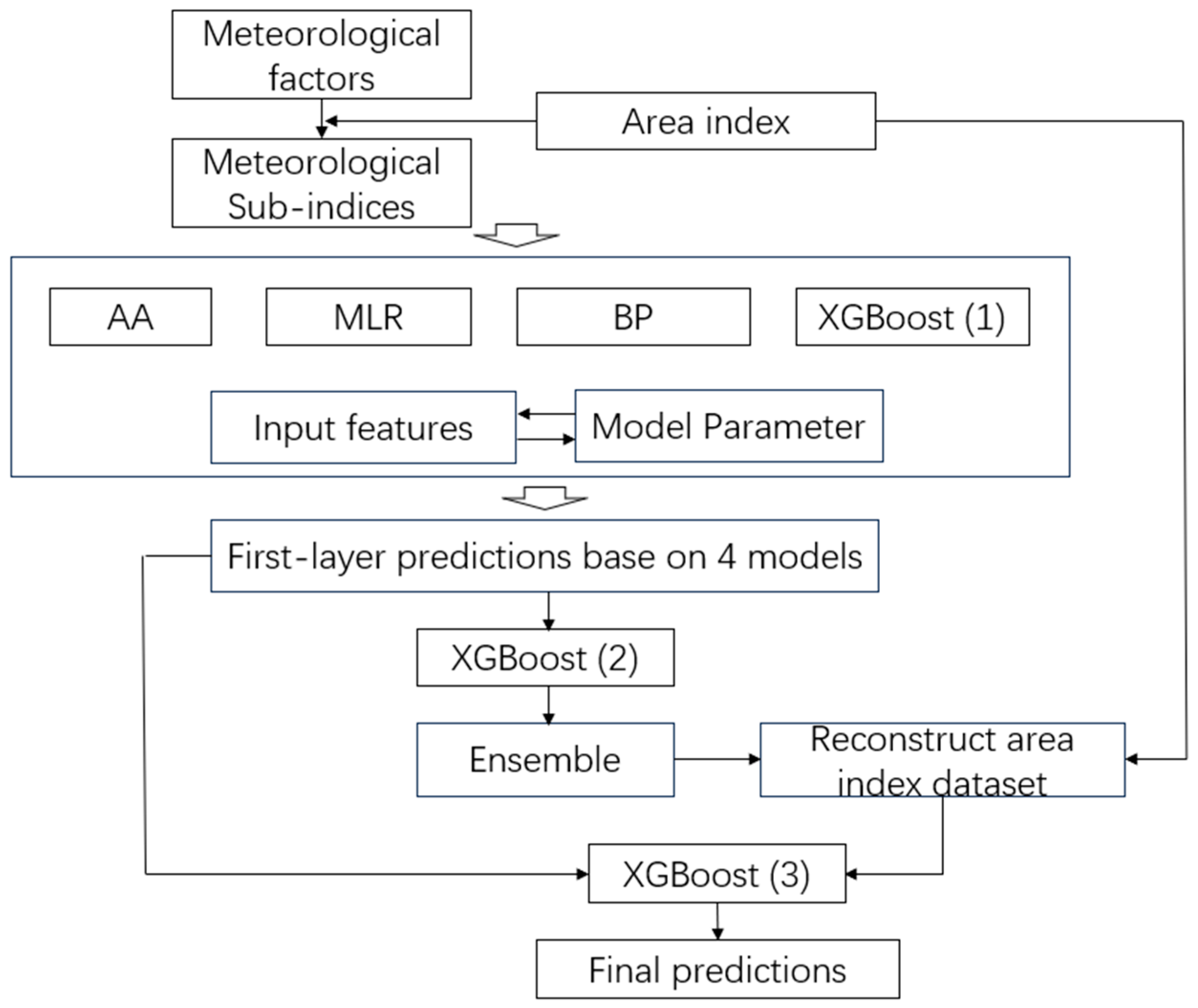
This study employs a stacking ensemble model based on multiple machine learning algorithms to construct the meteorological forecasting model for predicting the Lake Taihu cyanobacterial bloom area index. The stacking ensemble approach integrates multiple base models to enhance predictive performance, typically comprising a two-layer structure: the first layer consists of multiple mutually independent machine learning models, while the second layer utilizes their outputs as inputs to build a model that generates final predictions [31]. The comprehensive modeling procedure involves three sequential steps, which are illustrated in Figure 2.

(1) Four distinct models, additive index accumulation (AA), multiple linear regression (MLR), backpropagation neural network (BPNN), and extreme gradient boosting regression (XGBoost), are trained using the area index and meteorological sub-indices to generate preliminary predictions.

(2) An XGBoost model integrates the four first-layer predictions to produce refined outputs.

(3) To address temporal discontinuities in satellite-based area observations and enhance short-term forecasting capabilities, the predictions from step 2 are used to fill data gaps and then reconstruct area index dataset (including previous-day data). A final XGBoost model synthesizes the filled dataset with first-layer predictions.

The AA model aggregates selected meteorological sub-indices to form a comprehensive meteorological index K. This approach, widely adopted in atmospheric environmental research, is introduced here for cyanobacterial bloom forecasting. The methodology is formulated as:

$$K=\sum K_m$$

(4)

where $K_m$ is the meteorological sub-index for variable m, K represents a composite meteorological index derived from the additive aggregation of selected sub-indices.

The MLR model employs the least squares method to determine coefficients and intercept terms for selected meteorological sub-indices relative to the coverage index. This optimization minimizes the residual variance between predicted composite indices and observed area indices, thereby enhancing dimensional consistency and strengthening the indicative value of meteorological indices. The methodology is formulated as follows:

$$K={\beta }_0+\sum {\beta }_m{K}_m$$

(5)

where $K_m$ is the meteorological sub-index for variable m, ${\beta }_m$ is the regression coefficient for $K_m,{\beta }_0$ is the intercept term.

The BPNN model utilizes error backpropagation to train the relationship between meteorological sub-indices and the coverage index. As a multilayer feedforward neural network, BPNN operate through forward propagation of signals and backward propagation of errors. During forward propagation, input signals are processed layer-by-layer from the input layer through hidden layers to the output layer. If the output deviates from the expected value, error signals propagate backward to adjust weights across all layers [32].

XGBoost model is a supervised learning model that iteratively trains multiple weak learners to enhance predictive performance. It excels at capturing nonlinear relationships among variables through regularization (L1/L2) to control model complexity and prevent overfitting, Taylor-expansion approximation of the loss function (using first/second-order derivatives) for accelerated training and approximate greedy algorithms for optimal split point selection [33]. XGBoost is used in the 3 steps, and recorded as XGBoost (1), XGBoost (2), and XGBoost (3).

2.3.3. Model Parameters

This study employed grid search with 5-fold cross-validation to optimize parameters for both the BPNN and XGBoost models. Grid search systematically explores all predefined hyperparameter combinations to identify optimal configurations. In 5-fold cross-validation, the dataset is divided into five equal subsets. Iteratively, four subsets are used for training and one for validation, repeating this process until each subset has served as validation data.

BPNN comprises an input layer, two hidden layers, and an output layer. The input layer incorporates all aforementioned meteorological sub-indices. The output layer corresponds to the area index. The network contains two hidden layers with 39 and 13 neurons, respectively. Training specifications: 2500 iterations; loss function: Root Mean Square Error; learning rate: 0.01; L2 regularization applied; activation function: Rectified Linear Unit (ReLU); optimization method: Stochastic Gradient Descent.

Given the positively right-skewed distribution of the target variable in this study, the objective function for XGBoost is designated as ‘reg:gamma’. Other parameters are specified in

Table 2. XGBoost model parameter settings.

	XGBoost (1)	XGBoost (2)	XGBoost (3)
Number of Trees	200	150	100
Max Depth	4	2	2
Learning Rate	0.05	0.10	0.09
L2 Regularization Weight	1.00	1.00	1.00

.

2.3.4. Recursive Feature Elimination

This study employs Recursive Feature Elimination (RFE) to select optimal meteorological sub-indices combinations for training the four models in Step 1. RFE is a model-based feature selection method that iteratively trains models and removes the least important features to identify the optimal feature subset. Through successive rounds of model construction, features are progressively eliminated based on their performance contributions until all features have been evaluated. The elimination sequence directly reflects feature importance rankings, thereby facilitating the automatic selection of features that enhance both predictive accuracy and generalization capability. During RFE implementation, the coefficient of determination (R²) derived from 5-fold cross-validation was used to assess the performance of each feature subset.

2.4. Statistical Methods

The coefficient of determination (R²) was employed to statistically evaluate the correlation between predicted and observed area indices. Forecast accuracy was assessed based on whether the normalized area index exceeded 0.3. Correct prediction (Hit): Both forecast and observation values exceed 0.3, False negative: The forecast value is less than or equal to 0.3, while the observed value exceeds 0.3, False positive: The forecast value exceeds 0.3, while the observed value is less than or equal to 0.3.

$$R^2=1-{\displaystyle \frac{{(y_i-\widehat{y_i})}^2}{{(y_i-\overline{y})}^2}}$$

(6)

where $y_i$ is the observation date, $\widehat{y_i}$ is the prediction data, $\overline{y}$ is the mean of observation data.

Hit rate was also utilized to evaluate model performance. It is defined as the ratio of the number of correct predictions to the total number of observation values exceeding 0.3.

3. Results

3.1. Variation Characteristics of Cyanobacterial Bloom Coverage in Lake Taihu

Analysis of cyanobacterial blooms from 2016 to 2022 reveals that cyanobacterial blooms typically initiate in early May, with May–June representing the primary outbreak period. During July and August, the frequency and intensity of cyanobacterial blooms decrease due to increased precipitation and high temperatures. From September to November, cyanobacterial blooms area increases once more, reaching a secondary peaking in October, although overall intensity remains lower than during May–June. Bloom intensity declines markedly after mid-November, entering dormancy by December. The annual bloom coverage displays a clear bimodal pattern (Figure 3), with the most pronounced peak occurring in May. This observation indicates a significant shift compared to monitoring data from a decade ago, aligning with climate-driven changes in Lake Taihu’s bloom dynamics [26,34].

Interannual variations in cyanobacterial bloom outbreaks show significant differences across different years. From 2016 to July 2025, the most severe outbreak was recorded in 2017, reaching a maximum coverage of 1345 km², while 2023 saw the weakest manifestation at just 335 km². Annual occurrence rates also varied significantly: in 2017 and 2019, bloom area exceeded 50 km² on more than 50% of detectable days, contrasting sharply with 2023’s rate of only 10%. While some studies have reported the attenuated cyanobacterial blooms in 2023 and their causative factors [35], resurgence was observed in 2024 and 2025, with both years exhibiting peak area exceeding 400 km².

3.2. Correlations Analysis Between Meteorological Variables and Cyanobacterial Bloom Area in Lake Taihu

Table 3. Correlations between meteorological factors and cyanobacterial bloom surface area indices.

Meteorological Factors	Correlations with Meteorological Sub-Indices		Correlations with Meteorological Factors Values		Meteorological Factors	Correlations with Meteorological Sub-Indices		Correlations with Meteorological Factors Values
	Coefficient	Rank	Coefficient	Rank		Coefficient	Rank	Coefficient	Rank
08:00–14:00 mean wind speed (V1)	0.44	1	−0.41	1	Daily max wind speed (V16)	0.22	16	−0.21	13
08:00–14:00 wind speed variance (V2)	0.41	2	−0.29	2	Daily evaporation (V17)	0.21	18	0.25	8
Daily minimum 6-h wind speed variance (V3)	0.40	3	−0.28	5	Daily mean RH (V18)	0.18	19	0.20	14
08:00–14:00 wind direction variance (V4)	0.39	4	0.22	10	Previous-day max 6-h wind speed variance (V19)	0.17	20	−0.10	25
Daily maximum 6-h wind direction variance (V5)	0.36	5	0.22	12	Daily Precipitation (V20)	0.17	21	0.04	29
Daily mean wind direction variance (V6)	0.32	6	0.27	6	Daily min 6-h wind direction variation (V21)	0.16	22	0.14	22
Daily wind direction variance (V7)	0.32	7	0.16	18	Daily wind speed variance (V22)	0.15	23	−0.07	28
5-day accumulated temperature (V8)	0.31	8	0.28	4	Sunshine duration (V23)	0.14	24	−0.02	31
Daily minimum visibility (V9)	0.30	9	−0.15	19	Daily mean wind direction (V24)	0.14	25	−0.09	26
Daily mean temperature (V10)	0.28	10	0.29	3	Daily average air pressure (V25)	0.13	26	−0.25	9
Daily mean wind speed (V11)	0.28	11	−0.26	7	Daily average cloud cover (V26)	0.13	27	0.14	21
Precipitation in the previous 1–3 days (V12)	0.27	12	0.20	15	Previous-day max hourly wind speed variance (V27)	0.11	28	−0.14	20
Previous-day mean wind speed (V13)	0.25	13	−0.22	11	dAT (V28)	0.08	30	0.01	32
Daily max 6-h wind speed variance (V14)	0.25	14	−0.16	17	Daily max hourly wind speed variance (V29)	0.08	31	−0.13	23
Previous-day wind speed variance (V15)	0.23	15	0.04	30	Previous-day max hourly wind speed (V30)	0.06	32	−0.12	24

presents a comparison of the correlations between absolute values of various meteorological variables and the area index of cyanobacterial blooms in Lake Taihu. The strongest correlation was shown by the mean wind speed from 08:00–14:00 (r = −0.41), followed by the 08:00–14:00 wind speed variance, daily mean temperature, 5-day cumulative temperature, daily minimum 6-h variance, and daily mean wind direction variance. All these correlation coefficients had absolute values below 0.3. When comparing meteorological sub-indices with the cyanobacterial bloom area index in Lake Taihu, the mean wind speed from 08:00–14:00 showed the highest correlation (r = 0.44) again. This was followed sequentially by the 08:00–14:00 wind speed variance, daily minimum 6-h wind speed variance, 08:00–14:00 wind direction variance, daily maximum 6-h wind direction variance, and daily mean wind direction variance. Notably, all these correlation coefficients were above 0.3. Statistical processing of the meteorological data ensured that all correlations with the cyanobacterial bloom area index were positive. Additionally, meteorological sub-indices at each ranking position showed stronger correlations compared to their respective meteorological variables. This suggests that constructing meteorological sub-indices enhances their correlation with the cyanobacterial bloom area index in Lake Taihu.

The ranking of sub-indices by correlation strength with the cyanobacterial bloom area index differed from that of the absolute values of meteorological variables. Notably, the top seven correlated sub-indices all pertained to wind speed and direction. In contrast, the top seven absolute values of meteorological variables included parameters related to temperature. Analysis using meteorological sub-indices highlights that wind field variations, especially those measured by variance metrics, dominate short-term changes in cyanobacterial blooms in Lake Taihu. Conversely, the absolute values of correlation coefficients for cumulative and mean temperature showed minimal differences between results from meteorological sub-indices and those from raw meteorological data.

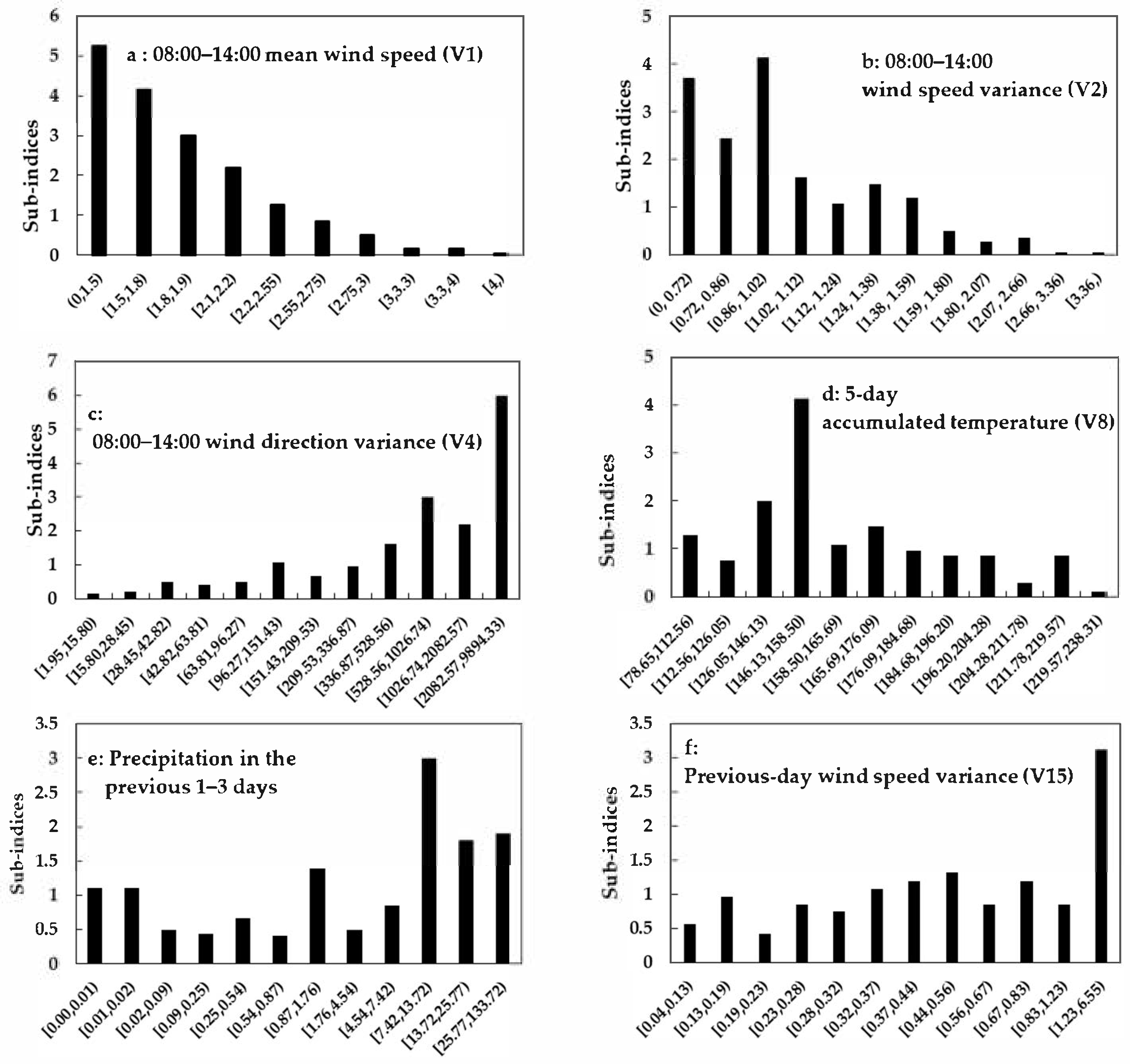
Figure 4 presents the value distribution of representative meteorological indices. These sub-indices decrease as wind speeds lower, increase with reduced wind speed variance, and rise with greater wind direction variance. The accumulated temperature over 7 days reaches its maximum within the range of 146.13–158.50 °C, indicating that moderate temperatures represent the most favorable conditions. High cyanobacterial bloom incidence occurs when the average temperature is near 30 °C. Increased precipitation in the preceding three days correlates with a higher likelihood of cyanobacterial blooms. Greater wind speed variance on the previous day also promotes cyanobacterial bloom formation.

3.3. Screening of Key Meteorological Sub-Indices

Given the large number of meteorological sub-indices established in this study, it is necessary to screen these indices to eliminate redundancy. This screening process aims to enhance the learning efficiency and performance of machine learning models. Figure 5 illustrates the change in the coefficient of determination (R²) following the stepwise elimination of input indices using the RFE method for the four models in Step 1.

Among the four models, the highest coefficient of determination (R²) was achieved by the XGBoost(1) model, reaching 0.403 after eliminating 14 variables. When all meteorological sub-indices were used, the R² values for the four models were similar, around 0.33. As feature variables were eliminated, the R² values gradually increased. The AA model reached its maximum R² of 0.365 after eliminating 9 indices. The BPNN model peaked at an R² of 0.392 after eliminating 13 indices. The MLR model reached its maximum R² of 0.375 after eliminating 15 indices. Throughout the process of reducing indices, the XGBoost (1) model consistently outperformed the other three models. Even when using only 7 meteorological sub-indices as inputs, the XGBoost (1) model maintained an R² of 0.370.

The optimal input meteorological sub-indices differed across models (

Table 4. The optimal combination of input indices based on recursive feature elimination method.

Models	Optimal Combination of Input Indices
AA	V2, V5, V4, V12, V19, V15, V20, V1, V8, V7, V9, V29, V25, V3, V10, V18, V27, V24, V28, V22, V26
MLP	V2, V5, V4, V15, V12, V10, V3, V1, V9, V25, V20, V7, V22, V29, V26, V28
BP	V4, V21, V12, V13, V8, V30, V15, V20, V7, V2, V22, V29, V27, V18, V10, V24, V19
XGBoost(1)	V2, V4, V1, V22, V5, V3, V8, V26, V10, V12, V27, V30, V23, V24, V15, V19, V20

Note: The meteorological sub-indices are sequenced according to the order of importance determined by the Recursive Feature Elimination method.

), but key indices also shared common characteristics, aiding in the identification of critical meteorological factors significantly impacting cyanobacterial bloom area in Lake Taihu. Specifically, V2, V4, V5 and V1 were consistently top-ranking across all four models. These results highlight that wind speed and direction are crucial meteorological factors influencing cyanobacterial blooms in Lake Taihu. Additionally, V12, V8 and V15 also played large roles in all four models. Moreover, some meteorological sub-indices with lower correlation rankings contributed significantly to model construction. For instance, V20 ranked 7th in the accumulation model, and V22 ranked 4th in the XGBoost (1) model.

3.4. Forecast Evaluation of Cyanobacterial Bloom Area Index in Lake Taihu

In Step 2 of model construction, the multi-model forecast result stacking model XGBoost (2) was employed. The 5-fold cross-validation coefficient of determination during model training reached 0.87, significantly higher than the optimal coefficient (0.40) obtained from the four models in Step 1. The results from XGBoost (2) and observational data were used to reconstruct the preceding-day observational dataset, with 42% of the data coming from observations and 58% from XGBoost (2) predictions. Step 3 utilized the reconstructed preceding-day observational data to predict the area index based on XGBoost (3). The 5-fold cross-validation coefficient of determination during training further improved to 0.90.

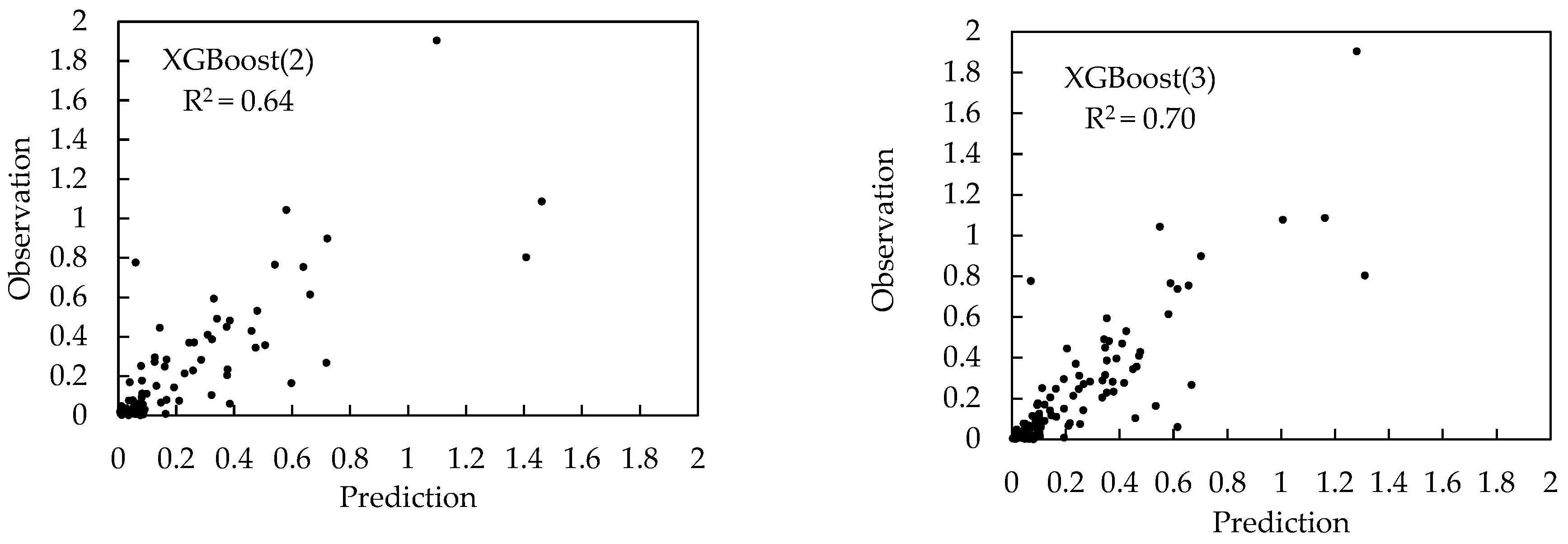
Using 2022 meteorological observation data, forecasts of cyanobacterial bloom area index were generated separately through XGBoost (2) and XGBoost (3) in the models (Figure 6). The coefficient of determination based on test data was lower than that from 5-fold cross-validation during modeling, but XGBoost (2) and XGBoost (3) reached 0.64 and 0.70, respectively. Regarding forecast accuracy (

Table 5. Verification of the Predictive Model for Cyanobacterial Bloom Area Index.

	Train Data The 5-Fold Cross-Validation Coefficient of Determination (R2)	Test Data (80)
		Deciding Coefficient (R2)	RMSE	>0.3 False Positive Rate	>0.3 False Negative Rate	>0.3 Hit Rate
XGBoost (2)	0.87	0.64	0.07	10%	5%	85%
XGBoost (3)	0.90	0.70	0.06	8%	5%	87%

Note: The correct rate, false negative rate, and false positive rate were evaluated using the criterion of whether the index exceeds 0.3.

), the hit rate for determining whether cyanobacterial bloom area exceeded 0.3 was over 85%. The false negative rate was around 5%, and the false positive rate was approximately 10%. XGBoost (3) demonstrated certain advantages over XGBoost (2) by reducing false positive rates.

3.5. Real-Time Forecast Verification of Cyanobacterial Bloom Area in Lake Taihu

Based on the China Meteorological Administration gridded meteorological forecasts [36], meteorological factor values are interpolated to each station to calculate the meteorological sub-indices. According to the prediction model constructed in this study, real-time forecasts of cyanobacterial bloom area index are generated. We use the observed area and forecasted area index from the previous day to convert the forecasted cyanobacterial bloom area indices for the next 7 days into actual bloom areas. This process allows us to further assess the model’s forecasting capability.

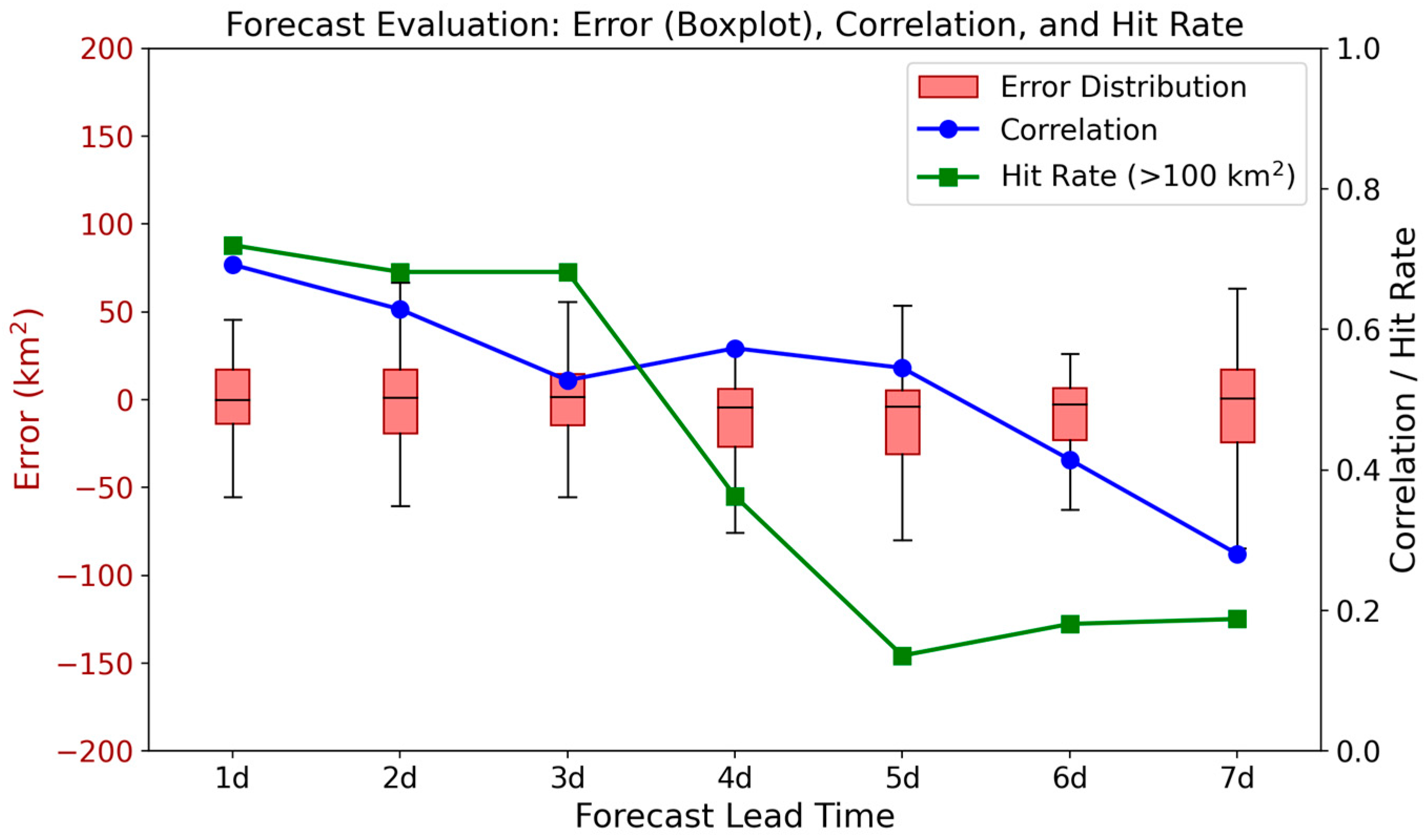
The performance of real-time cyanobacterial bloom area forecasts for Lake Taihu, covering the period from 2023 to July 2025, was evaluated. The correlation coefficient between forecast and observed bloom areas exceeded 0.6 for forecast lead times up to 2 days. A decline in correlation was observed from days 3 to 5, where coefficients averaged approximately 0.4. Further reduction occurred at longer lead times (days 6–7), with correlation coefficients averaging around 0.2 (Figure 7). During this period, 31 events with cyanobacterial bloom areas exceeding 100 km² were recorded (Figure 8). The model demonstrated considerable skill in forecasting whether the bloom area would exceed this threshold within 3 days. Hit rate exceeded 65% within this window, peaking at 72% for the 1-day lead time. However, model performance declined substantially beyond day 3, with hit rate falling to 36% on day 4 and remaining below 30% for lead times of 5–7 days.

4. Discussion

4.1. Impact of Key Meteorological Sub-Indices on Lake Taihu Cyanobacterial Bloom Area

Significant differences were observed among the key meteorological sub-indices selected during model construction. This variation may result from the inherent correlations between different meteorological sub-indices, alongside the fact that cyanobacterial blooms in Lake Taihu are driven by the combined effects of multiple meteorological factors [26]. Consequently, identifying a single dominant meteorological factor is challenging. However, a common set of key meteorological sub-indices was identified across the four models: Wind Speed Variance from 08:00–14:00, Wind Direction Variance from 08:00–14:00, Daily Maximum 6-h Wind Direction Variance, Wind Speed from 08:00–14:00, Precipitation Accumulation over the previous three days, 5-day Accumulated Temperature, and Wind Speed Variance on the previous day. These seven meteorological elements appear to be good indicators for predicting cyanobacterial bloom outbreaks. Although Precipitation Accumulation over the Previous 3 Days and Wind Speed Variance on the Previous Day ranked lower in correlation with the area index, they exert a greater influence on bloom outbreaks than some higher-ranking meteorological sub-indices.

Wind-field-related variables, such as wind speed and wind direction variance from 08:00 to 14:00, exhibit larger correlation coefficients with the Lake Taihu cyanobacterial bloom area index. Specifically, low wind speeds favor large-scale outbreaks of cyanobacterial blooms in Lake Taihu, a finding consistent with relevant studies [14,37]. However, within the models constructed in this study, wind speed variance and wind direction variance demonstrated greater importance than average wind speed; these two indices serve as crucial variables characterizing the spatiotemporal heterogeneity of the Lake Taihu wind field. The values of the wind speed variance and wind direction variance sub-indices reveal that smaller wind speed variance and larger wind direction variance facilitate cyanobacterial bloom outbreaks. Both wind speed variance and wind direction variance exhibit critical thresholds beyond which the probability of a cyanobacterial bloom outbreak in Lake Taihu significantly increases. The critical threshold for wind speed variance is approximately 1.02 m/s, and for wind direction variance, it is 528°. Smaller wind speed variance indicates more consistent wind speeds across the lake region, while larger wind direction variance signifies significant convergence or divergence within the wind field. Conditions of small wind speed variance and large wind direction variance typically occur when the wind field is weak and exhibits distinct convergence or divergence. Lake current convergence/divergence is a decisive factor influencing the dynamic changes in the spatial extent of Lake Taihu cyanobacterial blooms [16,38]. This study further confirms that wind speed and direction variance derived from meteorological observation data can effectively reflect the status of lake current convergence/divergence. Moreover, critical thresholds for their impact on cyanobacterial bloom area were identified.

Wind speed variance on the previous day was also identified as a key meteorological sub-index in the models. The sub-index values indicate that larger wind speed variance on the previous day favors cyanobacterial bloom outbreaks in Lake Taihu. Specifically, a critical threshold exists: when the wind speed variance on the previous day exceeds 1.23 m/s, the probability of a cyanobacterial bloom outbreak is more than three times higher than the average state. Qin et al. [16] indicated that during the cyanobacterial bloom outbreak stage in Lake Taihu, wind-wave action facilitates the rapid aggregation of cyanobacterial cells into large colonies, enabling them to float rapidly to the surface and form visible blooms when wind speed subsequently decreases [16]. Larger wind speed variance on the previous day suggests greater wind speed fluctuations, instability in the wind field, and larger wave variations within the Lake Taihu region during that period, which promotes the formation of large cyanobacterial colonies.

Current research presents some controversy regarding the impact of precipitation on cyanobacterial bloom outbreaks. Huang et al. [39] suggested a weak correlation between precipitation and the intensity of lake cyanobacterial blooms, potentially influenced by extreme precipitation events; Hang et al. [27] reported that precipitation can inhibit the occurrence of cyanobacterial blooms in Lake Taihu; while Zhu et al. [40] indicated that precipitation exerts multifaceted effects on cyanobacterial blooms in Lake Taihu. The results of this study demonstrate that precipitation accumulation over the previous three days has a considerable impact on cyanobacterial blooms in Lake Taihu. Precipitation within a certain intensity range appears favorable for bloom outbreaks, whereas precipitation on the same day shows minimal influence. The complexity of precipitation’s effect on Lake Taihu cyanobacterial blooms may arise because moderate antecedent precipitation can deliver more nutrients into the lake, while precipitation on the same day primarily acts as a flushing agent.

Numerous studies have pointed out that factors such as solar radiation and atmospheric pressure also strongly influence cyanobacterial bloom outbreaks. However, the results of this study did not highlight the impact of these elements. Specifically, their correlation coefficient ranks were both below 20th place, and their contributions to improving the composite index correlation coefficient were minor. This may be because factors like solar radiation primarily influence the process of cyanobacterial biomass accumulation [26]. Once cyanobacteria have resuscitated and accumulated sufficient biomass, solar radiation may no longer play a significant role in determining whether a large-scale bloom outbreak occurs. Given that this study primarily focuses on the short-term area changes in cyanobacterial blooms following resuscitation, the influence of solar radiation and other growth-promoting factors becomes less pronounced.

4.2. Analysis of Meteorological Forecast Performance for Lake Taihu Cyanobacterial Bloom Area Index

The forecast model based on stacked ensemble integration of multiple model results significantly outperformed single-model forecasts. In this study, the 5-fold cross-validated determination coefficient (R²) for the ensemble model XGBoost (2) increased to 0.87, compared to 0.40 for the single-model baseline. Incorporating observe data from the previous day further improved the model’s predictive performance, with XGBoost (3) achieving a 5-fold cross-validated R² of 0.90. Validation using observed data from 2022 as a test set yielded an R² of 0.70 for XGBoost (3), indicating good model generalization capability. While XGBoost (3) showed some improvement over XGBoost (2). However, the improvement was marginal, showing only about a 2% increase in prediction accuracy. Incorporating observational data contributed to the model learning process; however, since observational data was only available for 42% of the days, its effect on model improvement was limited. Nevertheless, utilizing observational data can reduce the model’s false positive rate, especially in real-time forecasting, where incorporating observations can improve forecasts for the next few days.

Based on real-time forecasts from 2023 to July 2025, the model demonstrated a 72% hit rate for 1-day lead predictions of Lake Taihu cyanobacterial bloom areas exceeding 100 km². This accuracy level is comparable to other methods [18,21]. Predictive performance degrades with increasing forecast lead time, mirroring the increase in bias observed in the gridded meteorological forecasts themselves. Within the first 1-day forecast window, gridded meteorological forecasts offer hourly resolution, allowing for more accurate calculations of parameters such as wind field variance. However, from day 2 onwards, the temporal resolution decreases to 3-h intervals, leading to a reduction in accuracy compared to the 1-day forecasts. Nevertheless, this methodology requires further refinement to enhance prediction accuracy.

The forecast model established in this study solely utilizes meteorological elements and cyanobacterial bloom area data, excluding variables such as nutrient concentrations and Chlorophyll-a concentrations. Consequently, the model lacks the capacity to reflect the influence of eutrophication levels on cyanobacterial blooms. However, since this study primarily focuses on short-term forecasts (1–3 days) of bloom area changes, it is noteworthy that lake eutrophication status shows relatively minor short-term variability. As a result, the model still demonstrated good performance despite the exclusion of these factors. These elements are crucial for constructing numerical models in other research contexts. Incorporating relevant observational data in future work will be beneficial for further improving the forecast capability for Lake Taihu cyanobacterial bloom outbreaks.

5. Conclusions

From 2016 to July 2025, the annual variation in Lake Taihu cyanobacterial bloom area exhibited a distinct bimodal pattern; the area peaked between May and June, with another notable but smaller peak around October. In 2023, the cyanobacterial bloom area was the smallest observed during this period. However, there was a noticeable increasing trend in recurrence in both 2024 and 2025.

Compared to the absolute values of meteorological elements, meteorological sub-indices constructed based on the probability distribution of these elements across different levels of Lake Taihu cyanobacterial bloom areas more accurately reflect the impact of meteorological factors on changes in the bloom area. Specifically, by employing the recursive feature elimination method, several key meteorological sub-indices have been identified as influencing changes in the cyanobacterial bloom area of Lake Taihu. These include: 08:00–14:00 wind speed variance, 08:00–14:00 wind direction variance, daily maximum 6-h wind direction variance, 08:00–14:00 wind speed, previous 3-day precipitation, 5-day accumulated temperature, and previous-day wind speed variance.

Wind speed variance and wind direction variance are important meteorological variables that characterize lake current convergence or divergence. Compared to average wind speed, these two variables exhibit greater importance within the model, offering more substantial indicative significance for predicting cyanobacterial blooms in Lake Taihu.

The forecast model based on stacked integration of multiple model results can effectively predict the short-term changes in the Lake Taihu cyanobacterial bloom area. Specifically, its 5-fold cross-validated determination coefficient reached 0.90, significantly higher than that of the single model. The determination coefficient between model results and test data reached 0.70.

Real-time forecasting results of Lake Taihu cyanobacterial blooms, based on meteorological elements from CMA gridded meteorological forecasts, show a hit rate of 72% for predicting bloom areas exceeding 100 km² one day in advance. The predictive performance for forecasts three days in advance shows overall good results, with hit rates all above 65%.

In the future, we will incorporate relevant observational data, including nutrient concentrations and Chlorophyll-a concentrations, to improve the forecast capability for Lake Taihu cyanobacterial bloom outbreaks. Furthermore, by leveraging gridded meteorological observations alongside cyanobacterial bloom distributions, we aim to develop more detailed forecasts of bloom distribution. This approach will enable us to provide more refined warnings regarding cyanobacterial blooms, significantly strengthening the foundation for sustainable water management in Lake Taihu.

References

1. Qin, B.; Gao, G.; Zhu, G.; Zhang, Y.; Song, Y.; Tang, X.; Xu, H.; Deng, J. Lake eutrophication and its ecosystem response. Chin. Sci. Bull. 2013, 58, 961–970. [Google Scholar] [CrossRef]
2. Kong, F.; Gao, G. Hypothesis on cyanobacteria bloom-forming mechanisam in large shallow eutrophic lakes. Acta Ecol. Sin. 2005, 25, 589–595. [Google Scholar] [CrossRef]
3. Huisman, J.; Codd, G.A.; Paerl, H.W.; Ibelings, B.W.; Verspagen, J.M.H.; Visser, P.M. Cyanobacterial blooms. Nat. Rev. Microbiol. 2018, 16, 471–483. [Google Scholar] [CrossRef]
4. Taranu, Z.E.; Gregory-Eaves, I.; Leavitt, P.R.; Bunting, L.; Buchaca, T.; Catalan, J.; Domaizon, I.; Guilizzoni, P.; Lami, A.; McGowan, S.; et al. Acceleration of cyanobacterial dominance in north temperate-subarctic lakes during the Anthropocene. Ecol. Lett. 2015, 18, 375–384. [Google Scholar] [CrossRef]
5. Michalak, A.M.; Anderson, E.J.; Beletsky, D.; Boland, S.; Bosch, N.S.; Bridgeman, T.B.; Chaffin, J.D.; Cho, K.; Confesor, R.; Daloğlu, I.; et al. Record setting algal bloom in Lake Erie caused by agricultural and meteorological trends consistent with expected future conditions. Proc. Natl. Acad. Sci. USA 2013, 110, 6448–6452. [Google Scholar] [CrossRef] [PubMed]
6. Yang, Z.; Li, Y.; Zhu, G.; Kang, H.; Li, N.; Zhang, Y.; Qin, B. Control factors of cyanobacterial bloom area in Lake Taihu, China (2003–2023). J. Lake Sci. 2025, 37, 734–751. [Google Scholar] [CrossRef]
7. Dai, Y.; Yang, S.; Zhao, D.; Hu, C.; Xu, W.; Anderson, D.M.; Li, Y.; Song, X.P.; Boyce, D.G.; Gibson, L.; et al. Coastal phytoplankton blooms expand and intensify in the 21st century. Nature 2023, 615, 280–284. [Google Scholar] [CrossRef] [PubMed]
8. Stumpf, R.D.; Johnson, L.T.; Wynne, T.T.; Baker, D.B. Forecasting annual cyanobacterial bloom biomass to inform management decisions in Lake Erie. J. Great Lakes Res. 2016, 42, 1174–1183. [Google Scholar] [CrossRef]
9. Qin, B.; Zhu, G.; Gao, G.; Zhang, Y.; Li, W.; Paerl, H.W.; Carmichael, W.W. A drinking water crisis in Lake Taihu, China: Linkage to climatic variability and lake management. Environ. Manag. 2010, 45, 105–112. [Google Scholar] [CrossRef]
10. Qin, B.; Li, W.; Zhu, G.; Zhang, Y.; Wu, T.; Gao, G. Cyanobacterial bloom management through integrated monitoring and forecasting in large shallow eutrophic Lake Taihu (China). J. Hazard. Mater. 2015, 287, 356–363. [Google Scholar] [CrossRef]
11. Yang, L.; Yang, X.; Ren, L.; Qian, X.; Xiao, L. Mechanism and control strategy of cyanobacterial bloom in Lake Taihu. J. Lake Sci. 2019, 31, 10. [Google Scholar] [CrossRef][Green Version]
12. Li, W.; Qin, B. Dynamics of spatiotemporal heterogeneity of cyanobacterial blooms in large eutrophic Lake Taihu, China. Hydrobiologia 2019, 833, 81–93. [Google Scholar] [CrossRef]
13. Qi, L.; Hu, C.; Visser, P.M.; Ma, R. Diurnal changes of cyanobacteria blooms in Lake Taihu as derived from GOCI observations. Limnol. Oceanogr. 2018, 63, 1711–1726. [Google Scholar] [CrossRef]
14. Shi, K.; Zhang, Y.; Zhou, Y.; Liu, X.; Zhu, G.; Qin, B.; Gao, G. Long-term MODIS observations of cyanobacterial dynamics in Lake Taihu: Responses to nutrient enrichment and meteorological factors. Sci. Rep. 2017, 7, 40326. [Google Scholar] [CrossRef] [PubMed]
15. Wang, S.; Zhang, X.; Chen, N.; Wang, W. Classifying diurnal changes of cyanobacterial blooms in Lake Taihu to identify hot patterns, seasons and hotspots based on hourly GOCI observations. J. Environ. Manag. 2022, 310, 114782. [Google Scholar] [CrossRef]
16. Qin, B.; Yang, G.; Ma, J.; Deng, J.; Li, W.; Wu, T.; Liu, L.; Gao, G.; Zhu, G.; Zhang, Y. Dynamics of variability and mechanism of harmful cyanobacteria bloom in Lake Taihu, China. Chin. Sci. Bull. 2016, 61, 759–770. [Google Scholar] [CrossRef]
17. Wu, T.; Yang, Z.G.; Qin, B.; Ma, J.; Yang, G. Movement of cyanobacterial colonies in a large, shallow and eutrophic lake: A review. Chin. Sci. Bull. 2019, 64, 3833–3843. [Google Scholar] [CrossRef]
18. Li, W.; Qin, B.; Zhu, G. Forecasting short-term cyanobacterial blooms in Lake Taihu, China, using a coupled hydrodynamic-algal biomass model. Ecohydrology 2014, 7, 794–802. [Google Scholar] [CrossRef]
19. Zhang, H.; Song, T.; Zhu, B.; Shi, J.; Zhang, J. Annual Forecast of the Extent of Cyanobacteria Bloom in Taihu Lake. Environ. Monit. China 2022, 38, 157–164. [Google Scholar] [CrossRef]
20. Park, Y.; Lee, H.K.; Shin, J.K.; Chon, K.; Kim, S.; Cho, K.H.; Kim, J.H.; Baek, S. A machine learning approach for early warning of cyanobacterial bloom outbreaks in a freshwater reservoir. J. Environ. Manag. 2021, 288, 112415. [Google Scholar] [CrossRef] [PubMed]
21. Pyo, J.; Cho, K.H.; Kim, K.; Baek, S.; Nam, G.; Park, S. Cyanobacteria cell prediction using interpretable deep learning model with observed, numerical, and sensing data assemblage. Water Res. 2021, 203, 117483. [Google Scholar] [CrossRef]
22. Ni, J.; Liu, R.; Tang, G.; Xie, Y. An Improved Attention-based Bidirectional LSTM Model for Cyanobacterial Bloom Prediction. Int. J. Control. Autom. Syst. 2022, 20, 3445–3455. [Google Scholar] [CrossRef]
23. Sandubete-López, J.; Fernandez-Fernandez, R.; Lopez-Orozco, J.A.; Risco-Martín, J.L. Shallow learning model for long-term cyanobacterial bloom forecasting in real-time monitoring system. Water Res. 2025, 287, 124283. [Google Scholar] [CrossRef]
24. Fournier, C.; Fernandez-Fernandez, R.; Cirés, S.; López-Orozco, J.A.; Besada-Portas, E.; Quesada, A. LSTM networks provide efficient cyanobacterial blooms forecasting even with incomplete spatio-temporal data. Water Res. 2024, 267, 122553. [Google Scholar] [CrossRef] [PubMed]
25. Binding, C.E.; Greenberg, T.A.; McCullough, G.; Watson, S.B.; Page, E. An analysis of satellite-derived chlorophyll and algal bloom indices on Lake Winnipeg. J. Great Lakes Res. 2018, 44, 436–446. [Google Scholar] [CrossRef]
26. Zhang, M.; Yang, Z.; Shi, X. Expansion and drivers of cyanobacterial blooms in Lake Taihu. J. Lake Sci. 2019, 31, 336–344. [Google Scholar] [CrossRef]
27. Hang, X.; Luo, X.; Xie, X.; Li, Y. Suitable Meteorological Indicators for Formation of Cyanobacteria Blooms in Lake Taihu. Meteor. Sci. Tec. 2019, 47, 171–178. [Google Scholar] [CrossRef]
28. Ma, R.; Kong, F.; Duan, H.; Zhang, S.; Kong, W.; Hao, J. Spatio-temporal distribution of cyanobacteria blooms based on satellite imageries in Lake Taihu, China. J. Lake Sci. 2008, 20, 687–694. [Google Scholar] [CrossRef]
29. Huang, Y.; Guo, B.; Sun, H.; Liu, H.; Chen, S.X. Relative importance of meteorological variables on air quality and role of boundary layer height. Atmos. Environ. 2021, 267, 118737. [Google Scholar] [CrossRef]
30. HJ 1098—2020; Technical Specifications for Monitoring and Evaluating Algal Bloom Based on Remote Sensing and Field Monitoring. China Environment Press: Beijing, China, 2020. Available online: https://www.mee.gov.cn/ywgz/fgbz/bz/bzwb/other/qt/202002/W020200213479102762551.pdf (accessed on 16 September 2025).
31. Wolpert, D.H. Stacked generalization. Neural Netw. 1992, 5, 241–259. [Google Scholar] [CrossRef]
32. Michael, A.N. Neural Networks and Deep Learning; Determination Press. 2015. Available online: http://neuralnetworksanddeeplearning.com/ (accessed on 16 September 2025).
33. Chen, T.; Guestrin, C.E. XGBoost: A scalable tree boosting system. In Proceedings of the 22nd ACM SIGKDD International Conference on Knowledge Discovery and Data Mining, San Francisco, CA, USA, 13–17 August 2016; pp. 785–794. [Google Scholar] [CrossRef]
34. Liu, X.; Zhang, G. A review of studies on the impact of climate change on cyanobacteria blooms in lakes. Adv. Water Sci. 2022, 33, 316–326. [Google Scholar] [CrossRef]
35. Song, T.; Zhang, H.; Xu, Y.; Dai, X.; Fan, F.; Wang, Y.; Liu, G. Cyanobacterial blooms in Lake Taihu: Temporal trends and potential drivers. Sci. Total Environ. 2024, 942, 173684. [Google Scholar] [CrossRef]
36. Hu, Z.; Xue, F.; Jin, R.; Sun, J.; Song, W.; Gao, B. Design and implementation of gridded forecast application platform. Meteorol. Mon. 2020, 46, 1340–1350. [Google Scholar] [CrossRef]
37. Luo, X.; Hang, X.; Cao, Y.; Hang, R.; Li, Y. Dominant meteorological factors affecting cyanobacterial blooms under eutrophication in Lake Taihu. J. Lake Sci. 2019, 031, 1248–1258. [Google Scholar] [CrossRef]
38. Ding, W.; Li, Y.; Xu, S.; Li, J.; Zhao, J.; Ruan, S.; Wang, Y. Characteristics of surface lake current and its effect on cyanobacteria migration in Lake Taihu under changing wind field. J. Hohai Univ. (Nat. Sci.) 2022, 50, 58–65. [Google Scholar] [CrossRef]
39. Huang, J.; Zhang, Y.; Arhonditsis, G.B.; Gao, J.; Chen, Q.; Peng, J. The magnitude and drivers of harmful algal blooms in China’s lakes and reservoirs: A national-scale characterization. Water Res. 2020, 181, 115902. [Google Scholar] [CrossRef]
40. Zhu, G.; Shi, K.; Li, M.; Li, N.; Zou, W.; Guo, C.; Zhu, M.; Xu, H.; Zhang, Y.; Qin, B. Seasonal forecast method of cyanobacterial bloom intensity in eutrophic Lake Taihu, China. J. Lake Sci. 2020, 32, 11. [Google Scholar] [CrossRef]
Figure 1. Location map of the meteorological monitoring sites (red dots) and the spatial distribution of cyanobacterial bloom frequency (the ratio of observed cyanobacterial bloom days to valid observation days, i.e., cloud-free days) from 2016 to July 2025 in the Lake Taihu, China.
Sustainability 17 08376 g001
Figure 2. The framework of the stacking ensemble model (AA is the additive index accumulation model, MLR represents the multiple linear regression model, BPNN represents the backpropagation neural network model, and XGBoost is the extreme gradient boosting regression model).
Sustainability 17 08376 g002
Figure 3. Monthly (left) and annual (right) variations in cyanobacterial surface bloom areas in Lake Taihu from 2016–July 2025.
Sustainability 17 08376 g003
Figure 4. The value of typical meteorological sub-indexes ((a): average wind speed from 08:00 to 14:00, (b): wind speed variance from 08:00 to 14:00, (c): wind direction variance from 08:00 to 14:00, (d): accumulated temperature for 5 days, (e): precipitation in the previous 3 days, (f): wind speed variance in the previous day).
Sustainability 17 08376 g004
Figure 5. Variation in deciding coefficient with the variable selection using Recursive feature elimination method.
Sustainability 17 08376 g005
Figure 6. The predictive and observed data for 2022.
Sustainability 17 08376 g006
Figure 7. Forecast verification for the cyanobacteria bloom area over the leading 1–7 days (the blue line represents the correlation coefficient between forecasted and observed areas, the green line indicates the hit rate for events where the cyanobacteria bloom area exceeds 100 km2, and the boxplot shows the distribution of errors).
Sustainability 17 08376 g007
Figure 8. Forecast and observed values of cyanobacterial bloom area for Lake Taihu from 2023 to July 2025 at the 1-day lead time.
Sustainability 17 08376 g008