Abstract
Among various natural hazards, floods stand out due to their frequency and severe impact on society and the environment. This study aimed to develop a flood susceptibility model for Demak District, Indonesia, by integrating remote sensing data, machine learning techniques, and CMIP6 Global Climate Model (GCM) data. The approach involved mapping current flood susceptibility using Sentinel-1 SAR data as the flood inventory and applying machine learning algorithms such as MLP-NN, Random Forest, Support Vector Machine (SVM), and XGBoost to predict flood-prone areas. Additionally, future flood susceptibility was projected using CMIP6 GCM precipitation data under three Shared Socioeconomic Pathway (SSP) scenarios (SSP1-2.6, SSP2-4.5, and SSP5-8.5) covering the 2021–2100 period. To enhance the reliability of future projections, a multi-model ensemble approach was employed by combining the outputs of multiple GCMs to reduce model uncertainties. The results showed a significant increase in flood susceptibility, especially under higher emission scenarios (SSP5-8.5), with very high susceptibility areas growing from 16.67% in the current period to 27.43% by 2081–2100. The XGBoost model demonstrated the best performance in both current and future projections, providing valuable sustainable planning insights for flood risk management and adaptation to climate change.
1. Introduction
Floods are among the most frequent hydrometeorological disasters, causing significant environmental, social, and economic impacts worldwide [1]. They lead to infrastructure damage, socioeconomic disruption, and environmental degradation [2,3]. Over the past two decades, flood events have increased by 40%, driven by changing weather patterns and environmental stressors such as deforestation, land degradation, urbanization, and population growth [4,5]. These disasters are influenced by complex meteorological, hydrological, geomorphological, and topographical factors, which are often exacerbated by unsustainable human activities [6].
Human-induced greenhouse gas emissions, resulting from activities such as fossil fuel combustion, deforestation, and livestock farming, have intensified climate change since the mid-19th century [7,8]. Climate change manifests in various forms, including rising temperatures, rising sea levels, increased droughts, and increased flooding [9]. Evidence increasingly links climate change to more frequent extreme precipitation and rising sea levels, especially affecting coastal and low-lying areas [10,11]. Accurate flood prediction and strategic intervention are therefore essential to reduce socio-economic losses. This aligns with Sustainable Development Goal (SDG) 13, which emphasizes the urgency of addressing climate-related hazards such as flooding [12]. Changes in precipitation patterns are a major flood driver [12], and urbanization increases flood risks by expanding impervious surfaces and reducing infiltration [13]. Thus, understanding future flood risks and their contributing factors is crucial, and incorporating future climate scenarios, particularly precipitation projections, can enhance mitigation and adaptation strategies. Numerous Global Climate Models (GCMs) have been developed to simulate future climate scenarios and support the IPCC’s reports [14]. The latest CMIP6 initiative advances previous frameworks by offering coordinated simulations with improved spatial and temporal resolution, forming the scientific basis of the IPCC’s Sixth Assessment Report [15,16,17]. CMIP6 includes five Shared Socioeconomic Pathways (SSPs) that reflect different global development and emission trajectories, and the use of SSP-based GCM outputs is valuable in assessing future flood risks and informing adaptation planning [18,19].
A flood susceptibility model (FSM) identifies areas prone to flooding based on regional geographical and hydrometeorological characteristics and helps to map flood-prone zones and to guide mitigation strategies [20]. Common FSM methods include physically based models, multi-criteria decision making (MCDM), statistical approaches, and machine learning (ML) techniques [21]. While physically based models are detailed, they often face data availability challenges [22]. Similarly, MCDM, such as AHP, relies on expert judgment, introducing subjectivity [23]. Likewise, statistical methods such as logistic regression and frequency ratio are widely used but assume linearity, which limits their effectiveness in capturing flood complexity [21,24]. In contrast, machine learning has emerged as a robust alternative due to its ability to process complex, non-linear patterns and large datasets, including variables such as precipitation, slope, and land use [25,26]. Reliable FSMs require historical flood records, commonly in the form of flood inventory maps [27,28]. While field surveys offer precise data, they are limited by accessibility, time, cost, and scale [29]. Remote sensing, especially using Sentinel-1 SAR, offers a practical, timely, and extensive alternative for flood inventory development, overcoming many limitations of field-based approaches [30].
This study is motivated by the need to assess how climate change will influence flood susceptibility across space and time. While climate data from the Coupled Model Intercomparison Project Phase 6 (CMIP6) are widely used to evaluate future precipitation trends, their application in predictive flood mapping remains limited. Very few studies integrate CMIP6 GCM outputs with machine learning and remote sensing to generate forward-looking flood susceptibility maps. This study addresses that gap by incorporating precipitation projections from CMIP6 Global Climate Models (GCMs) under three different Shared Socioeconomic Pathways (SSP1 2.6, SSP2-4.5, and SSP5-8.5). These are used to project future flood susceptibility patterns under varying climate change scenarios.
The first objective is to develop a flood susceptibility model using Sentinel-1 SAR data as a flood inventory for current flood susceptibility modeling. This involves improving the mapping approach by combining Sentinel-1 SAR-derived flood data with other remote sensing inputs and applying machine learning algorithms such as Random Forest, MLP-NN, XGBoost, and Support Vector Machine. The second objective is to predict future flood susceptibility in Demak District using CMIP6 GCM precipitation data under various climate change scenarios, enabling an assessment of how flood risk may evolve over time. The third objective is to evaluate the impact of different climate change scenarios (SSP1-2.6, SSP2-4.5, and SSP5-8.5) on flood susceptibility, providing insights into how emissions pathways and climate dynamics contribute to long-term flood risk, thereby supporting adaptive sustainable development spatial planning and flood mitigation efforts in data-scarce regions.
2. Materials and Methods
2.1. Study Area
Demak District is located in the north of Central Java Province, Indonesia, is geographically situated between the coordinates of 6°43′26″–7°09′43″ South Latitude and 110°27′58″–110°48′47″ East Longitude. The area is approximately 995.32 km2 or 2.76 percent of the total area of Central Java, and consists of 14 sub-districts (Figure 1). It borders the Java Sea to the north, Kudus and Grobogan District to the east, Semarang District to the south, and Semarang City to the west. According to the Koppen-Geiger climate classification, Demak has a tropical monsoon climate (Am) as shown in Figure 2, with precipitation varying from 375 mm to 2436 mm per year [31]. The majority of the population are farmers, with a total population of around 1.12 million and an average population density of 1246 people per km2.
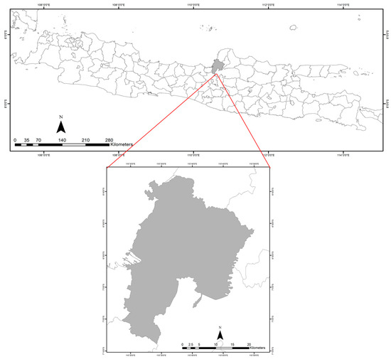
Figure 1.
Demak District as the study location within Central Java.
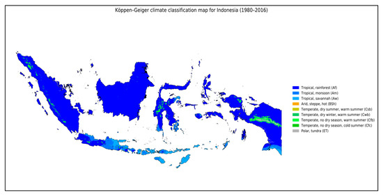
Figure 2.
Overview of climate classification in Indonesia according to the Koppen-Geiger during period 1980–2016.
2.2. Datasets
This study incorporated several data types from satellite remote sensing (Table 1) and CMIP6 GCM data (Table 2). Due to the absence of field survey-based flood inventory data, flood data from mapping results using Sentinel-1 SAR were used to construct the flood inventory. Data pre-processing was conducted both in Google Earth Engine and ArcMap 10.8 (accessed on 1 October 2024). The data were then used to generate current and future flood susceptibility models.

Table 1.
Summary of spatial datasets and resolutions applied in this study.
Table 2.
Overview of Sentinel-1A image acquisition during March 2024 flood in Demak District.
2.2.1. Flood Inventory Map
A flood inventory map was reconstructed via Sentinel-1 Synthetic Aperture Radar (SAR) imagery using the Otsu method, thus allowing for the reliable detection of inundated areas regardless of cloud cover [32,33]. To validate the accuracy of the flood inventory generated from the Sentinel-1 SAR data, flood extent maps provided by UNOSAT for the March 2024 flood event were used as a reference. A visual and spatial comparison confirmed a high degree of correspondence between the SAR-derived inundation areas and the UNOSAT delineations, with an accuracy of more than 89.00. Given the lack of comprehensive field data, this secondary validation supports the reliability of the flood inventory used in model training. A time-series analysis of the SAR data captured the flooding during major events, particularly the severe flood that struck Demak District on 13 March 2024, triggered by intense rainfall and the collapse of the Wulan River embankment (Table 2).
Figure 3 depicts the dynamics of flood inundation in Demak District, detected using Sentinel-1 SAR imagery with the Otsu thresholding method. The detection was performed by comparing the backscatter values before and during the flood, where a decrease in the backscatter value indicates an inundated area [34,35]. Visualizations on 15, 19, 27, and 31 March show changes in the flood distribution over time.
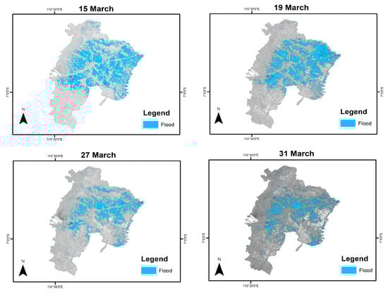
Figure 3.
Dynamic flood captured based on Otsu thresholding overlay with different backscatter coefficients.
This flood lasted for more than one month and was the most devastating flood in the last 30 years. The disaster caused widespread impacts, including crop failure across 4299 hectares of rice fields and the displacement of over 25,000 people, and affected more than 95,000 residents. A composite inundation map representing the maximum flood extent was generated by aggregating the four Sentinel-1 SAR captures from March 2024. Based on this composite map, a total of 450 flood and non-flood data points were then obtained via stratified random sampling, as shown in Figure 4. In total, 80% of the data were allocated for training and the remaining 20% for testing, while 25% of the training data were further set aside for validation purposes.
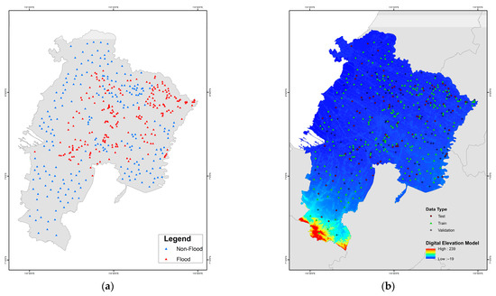
Figure 4.
Flood and non-flood points (a): training, validation, and testing datasets (b).
2.2.2. Flood Conditioning Factors
The selection of appropriate variables before use for flood susceptibility modeling analysis is crucial because it will affect the accuracy of the flood hazard map results [36,37]. Indicators that are considered as variables need to be analyzed, and their effects on the influence of flood events should be visualized. In this study, 14 flood predictors were carefully selected based on data availability and a literature review of previous studies [38,39]. Incorporating many flood conditioning factors, including topographic, hydrological, and geo-environmental data, will improve the accuracy of the flood susceptibility models generated via machine learning. A large number of predictors in a flood susceptibility model improves the model’s ability to detect flood-prone areas but also brings challenges related to model complexity and interpretation of the results [40]. The selection of relevant and appropriate predictors is crucial to ensure reliable and useful results. A total of 14 flood conditioning factors were selected in this research.
Flood susceptibility is affected by a range of topographic, hydrological, and environmental factors (Figure 5 and Figure 6). Elevation plays a vital role, as low-lying areas are more prone to water accumulation and river overflow, while steep slopes promote runoff and reduce pooling [41,42]. Slope further determines the speed and direction of water flow, with steep slopes facilitating rapid drainage, whereas gentle slopes increase flood potential [43,44]. Aspect, or slope orientation, affects microclimates and moisture retention; shaded slopes retain more water, increasing susceptibility [45]. Curvature of the land influences whether water tends to accumulate (concave areas) or drain quickly (convex areas), affecting flood formation and erosion [46].
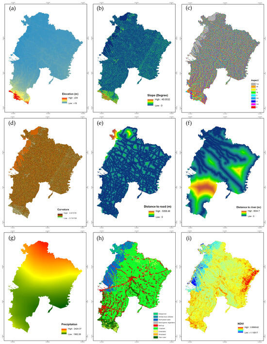
Figure 5.
Flood conditioning factors: (a) elevation, (b) slope, (c) aspect (d) curvature, (e) distance to road, (f) distance to river, (g) precipitation, (h) land use land cover (LULC), and (i) Normalized Different Vegetation Index (NDVI).
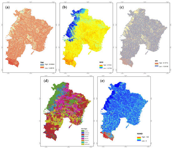
Figure 6.
Flood conditioning factors: (a) Topographic Wetness Index (TWI), (b) Normalized Different Soil Index (NDSI), (c) Stream Power Index (SPI), (d) soil type, and (e) height above nearest drainage (HAND).
The Topographic Wetness Index (TWI) estimates potential water accumulation based on slope and catchment area, with high values indicating areas vulnerable to water pooling [47]. The TWI equation is shown below:
Distance to river (DTRiver) is another key factor, as proximity to rivers increases exposure to overflow, particularly in flat or low-lying zones [48]. Similarly, distance to road (DTRoad) influences flood risk depending on infrastructure presence; roads may offer drainage or act as barriers, while remote areas lacking infrastructure are more vulnerable [49]. Land use land cover (LULC) impacts water absorption and runoff behavior. Urban areas, due to impervious surfaces, exacerbate runoff and flood risk, while vegetated regions mitigate it [50]. The year 2023 was chosen for the LULC period. The Normalized Difference Vegetation Index (NDVI) assesses vegetation health, where high NDVI reduces runoff and low NDVI, often in urbanized or deforested zones, increases flood susceptibility [51,52]. This study used NDVI in the December 2023 period.
Precipitation is a direct flood trigger; intense or prolonged precipitation overwhelms drainage, leading to inundation, especially where soil saturation is high [53]. In this study, we used precipitation during the 2015–2024 period. The Stream Power Index (SPI) measures the erosive energy of flowing water. High SPI indicates stronger water forces capable of causing erosion and flooding in steep terrain [54].
Soil type is also critical, as it determines infiltration capacity; permeable soils reduce runoff, while compacted or clay-rich soils increase it [55]. The Normalized Difference Soil Index (NDSI) provides insight into soil moisture, with lower values associated with wetter soils and increased flood risk [56]. The year 2023 was selected as the NDSI mapping period.
Lastly, the height above nearest drainage (HAND) calculates elevation relative to drainage points; lower HAND values indicate greater susceptibility due to proximity to water channels [57,58].
2.2.3. CMIP6 Global Climate Models (GCMs)
This study used climate projection data from 12 GCMs developed by various international climate research institutions. To ensure reliability, historical data (1991–2014) were compared with gauge station observations for validation. Future projections (2020–2100) were based on three Shared Socioeconomic Pathway (SSP) scenarios, as shown in Table 3: SSP1-2.6, SSP2-4.5, and SSP5-8.5. All climate data were downloaded from the WorldClim website (https://www.worldclim.org/ (accessed on 2 October 2024)) and NASA Earth Exchange Global Daily Downscaled Projections (NEX-GDDP-CMIP6) website (https://nex-gddp-cmip6.s3.us-west-2.amazonaws.com/index.html (accessed on 2 October 2024)). CMIP6 GCM data are shown in Table 4. These datasets were used to generate precipitation projections, which were then integrated into the flood susceptibility modeling framework to assess future flood risks under different climate scenarios.
Table 3.
Three different scenarios and their descriptions.
Table 4.
The CMIP6 (Coupled Model Intercomparison Project Phase 6) GCM dataset.
2.2.4. Gauge Station
In Table 5, three precipitation gauge stations—Brumbung, Bungo, and Jatisono—were used to validate the historical outputs of the selected GCMs. The observed precipitation data from these stations were obtained from the Indonesian Meteorological, Climatological, and Geophysical Agency (BMKG) through its official portal website (https://dataonline.bmkg.go.id/dataonline-home (accessed on 1 October 2024)).
Table 5.
Gauge stations in Demak District.
Due to data availability, the data covered the period 1991–2014 (24 years) and served as a reference for assessing the accuracy of GCM simulations. This validation process ensured that the climate models used in this study accurately represented historical precipitation patterns in the study area.
2.3. Methods
This study was conducted in two main steps (Figure 7). The first step focused on generating a current flood susceptibility model using 14 flood conditioning factors, flood inventory data (225 flood and 225 non-flood points), and Sentinel-1 SAR imagery. The influencing factors were selected based on their variance inflation factors (VIFs) and tolerance, and then, machine learning modeling (MLP-NN, RF, SVM, and XGBoost) was performed to produce the current flood susceptibility model. To enhance model robustness and generalizability, a 5-fold cross-validation strategy is implemented, ensuring that each subset of the data is used for both training and validation. In addition, hyperparameter optimization is carried out using GridSearchCV for each algorithm to fine-tune model settings and maximize predictive accuracy. Finally, the SHAP (SHapley Additive exPlanations) method was used to interpret the results and explain the contribution of each factor to the flood susceptibility predictions generated by the model.
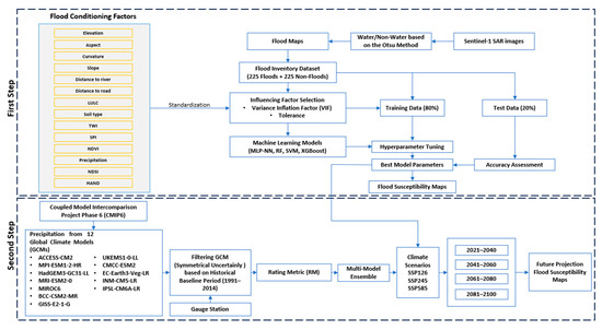
Figure 7.
This study’s research methodology.
The second step aimed to project future flood susceptibility by utilizing precipitation data from 12 CMIP6 GCMs. These models were filtered using symmetrical uncertainty and evaluated using the Rating Metric (RM). GCMs with RM scores above 0.70 were selected and combined into a multi-model ensemble, which was applied to future climate scenarios (SSP126, SSP245, and SSP585) across four time periods (2021–2040, 2041–2060, 2061–2080, and 2081–2100) to generate future flood susceptibility projections. To ensure spatial consistency for the modeling process, all raster datasets were resampled to a uniform spatial resolution of 30 m.
2.3.1. Multicollinearity Analysis
A multicollinearity analysis identifies collinearity among conditioning factors [59]. Two indices were used in this analysis: variance inflation factor (VIF) and tolerance. The purpose of a multicollinearity analysis in flood susceptibility modeling is to identify and eliminate high correlations among independent predictor variables that may distort model interpretation [60]. By reducing multicollinearity, the analysis ensures more reliable and accurate assessment of each variable’s contribution to flood risk. These indices can be calculated using the following equations:
where is the coefficient of determination of the -th independent variable on all the other independent variables.
In this study, a VIF threshold of less than 5 and a tolerance threshold of more than 0.1 were used to identify the presence of multicollinearity [61]. Variables that met these criteria were considered suitable to be used as flood conditioning factors.
2.3.2. Machine Learning Models
Four machine learning models were used to develop the flood susceptibility maps. MLP-NN, Random Forest, Support Vector Machine, and XGBoost were selected due to their complementary strengths in handling nonlinear relationships, high-dimensional feature spaces, and imbalanced datasets commonly encountered in geospatial flood susceptibility modeling.
MLP-NN
A Multilayer Perceptron Neural Network (MLP-NN) is a widely utilized feedforward artificial neural network architecture for classification. Its structure consists of an input layer, one or more hidden layers, and an output layer, with interconnected neurons that use non-linear activation functions [62]. MLPs are capable of approximating complex, non-linear functions by learning from data through a supervised process such as backpropagation [63].
Random Forest
Random Forest (RF) is an ensemble learning method that constructs a multitude of decision trees, with each tree trained on a random subset of the data (bagging) [64]. By using a random subset of features at each node, the model introduces diversity among the trees, which helps to reduce overfitting and improve generalization performance [65]. The final prediction is an aggregated result from all trees, leading to superior accuracy and robustness compared to a single decision tree [66].
Support Vector Machine (SVM)
A Support Vector Machine (SVM) is a supervised learning technique that performs classification by finding the ideal hyperplane that maximally separates data points into different classes [67]. To handle non-linearly separable data, SVM uses kernel functions to transform the data into a higher-dimensional space, which enhances its generalization performance [68].
XGboost
Extreme Gradient Boosting (XGBoost) is a robust and efficient ensemble learning algorithm based on the gradient boosting framework [69]. It sequentially adds models typically decision trees that correct the errors of their predecessors to enhance predictive performance [70]. To prevent overfitting and improve generalization, XGBoost employs built-in regularization methods, making it highly effective for large datasets.
2.3.3. Evaluation Metric
To systematically evaluate machine learning model performance, this study employs several classification metrics, including accuracy, precision (PPV), recall (sensitivity), specificity, negative predictive value (NPV), F1-score, and Cohen’s Kappa [71,72]. The Area Under the Receiver Operating Characteristic Curve (AUC), along with its 95% confidence interval, is used to assess the discriminatory power of the models, while asymptotic significance values are reported to confirm the statistical validity.
2.3.4. Symmetrical Uncertainty
Symmetrical uncertainty (SU) is an entropy-based filtering selection method used to evaluate the similarity between observed data and Global Climate Model (GCM) outputs in time series form [73,74]. It relies on information entropy principles to assess mutual information, where the mutual entropy between two variables X and Y is calculated using their joint and marginal probability distributions. The information gain (IG) quantifies how much knowledge of Y reduces the uncertainty in X and is defined as the difference between the entropy of X and the joint entropy of X and Y [75].
Since IG is scale-sensitive, it is normalized using the entropies of both variables, resulting in the symmetrical uncertainty (SU) metric:
This metric yields values between 0 (no similarity) and 1 (perfect similarity), providing a balanced and scale-independent measure of how closely GCM data resemble observed climate records [73].
The results of GCM performance across the three gauges station, Brumbung, Bungo, and Jatisono, are presented in Table 6. The analysis shows that IPSL had the highest SU values at Brumbung (0.87) and Jatisono (0.83), indicating strong agreement with the observed data. MIROC6 ranked first at Bungo (0.85) and performed well at the other stations (Brumbung: 0.82, Jatisono: 0.76). EC-EARTH consistently achieved high scores across all stations, with 0.85 (Brumbung), 0.85 (Bungo), and 0.74 (Jatisono). Furthermore, BCC showed strong performance at Brumbung (0.85) and Bungo (0.81), but a lower SU of 0.72 at Jatisono. MRI consistently had the lowest SU scores 0.80 (Brumbung), 0.75 (Bungo), and 0.72 (Jatisono), indicating relatively weak similarity with observed precipitation patterns.
Table 6.
Symmetrical uncertainty result in three different gauge stations.
2.3.5. Rating Metric
After evaluating the performance of the twelve GCMs using the symmetrical uncertainty (SU) method at three gauges stations in Demak District, the Rating Metric (RM) approach was applied to assess the spatial consistency of each GCM across the stations. The Rating Metric (RM) quantifies the overall spatial consistency of each GCM by averaging its rankings across multiple stations, as defined by the following equation [76]:
where n represents the number of GCMs, and Rank1 to Rankₙ are the SU-based ranks of each GCM at each station. The RM score ranges from 0 to 1, with 1 indicating excellent spatial consistency and 0 indicating poor performance [77].
Based on the results shown in Table 7, IPSL recorded the highest Rating Metric (RM) score of 0.83, with an average rank of 2 across the Brumbung, Bungo, and Jatisono stations, indicating superior spatial consistency and overall performance. MIROC6 and EC-EARTH followed, with RM scores of 0.81 and 0.78, respectively, also showing strong agreement with the observed precipitation data. In contrast, models such as UKEMS (RM = 0.03), HADGEM (RM = 0.06), and CMCC (RM = 0.17) showed the lowest scores, reflecting poor spatial correlation. In line with common practice in GCM evaluation studies, a threshold of RM > 0.70 was adopted to select models for the ensemble. These results confirm that IPSL, MIROC6, and EC-EARTH are the most consistent and reliable GCMs for representing precipitation patterns in the study area.
Table 7.
Overall Rating Metric score.
2.3.6. Multi-Model Ensemble
Following the application of the Rating Metric (RM) method to assess GCM performance, a multi-model ensemble (MME) was constructed to improve the reliability and reduce the uncertainty among models of precipitation projections [78,79]. By combining the outputs of several Global Climate Models (GCMs), this method helps to mitigate the biases and limitations inherent to individual model [80,81,82]. The ensemble comprises GCMs with RM scores above 0.70, with IPSL, MIROC6, and EC-EARTH showing strong spatial agreement with the observed data. To assign relative importance to each model, normalized weights were calculated by dividing each model’s RM score by the total RM of the top three models. These weights were then applied to generate the ensemble output ) through a weighted average of individual model outputs. The formula is shown below:
2.3.7. Multi-Model Ensemble Evaluation
The performance of the model was assessed using several statistical indicators, including the Pearson correlation coefficient , Nash–Sutcliffe Efficiency , Root Mean Square Error , and index of agreement . The equations are given in the following equation:
The Pearson correlation coefficient , which ranges from −1 to 1, indicates the strength of the linear relationship between the observed and simulated values. Values closer to 1 signify a strong correlation. The Nash–Sutcliffe Efficiency ranges from to 1, where values above 0.5 suggest acceptable model performance. Root Mean Square Error measures the average magnitude of prediction errors in the same units as the observed data, with lower values indicating better accuracy. The index of agreement reflects the average bias between the predicted and observed values, where values close to 1 indicate perfect agreement.
3. Results
3.1. Multicollinearity Analysis
Multicollinearity analyses are a crucial step in the pre-modeling phase of a flood susceptibility model. Table 8 shows the scores for both the VIF and tolerance values across all 14 variables. SPI has the highest value for VIF, with a score of 3.553, and a tolerance of 0.281. Since all variables have a VIF of less than 5 and a tolerance of more than 0.1, it indicates that there is no significant multicollinearity. Therefore, they can be used as flood conditioning factors in the flood susceptibility model.
Table 8.
Multicollinearity analysis results.
3.2. Feature Importance
After confirming the absence of significant multicollinearity among flood conditioning factors, this study proceeded to assess the relative influence of each variable on flood susceptibility. A feature importance analysis was performed using four machine learning algorithms, MLP-NN, Random Forest, SVM, and XGBoost to identify the most dominant factors influencing flood susceptibility in the study area.
Figure 8 shows the feature importance analysis, which revealed variations in the contribution of flood conditioning factors across the four machine learning models. Elevation, DTRoad, LULC, and precipitation consistently emerged as key variables across models, indicating that topography, land use, infrastructure, and precipitation patterns are crucial in predicting flood susceptibility in Demak District. The differing rankings reflect the varied sensitivity of each algorithm to environmental factor interactions and due to the different ways algorithms like tree-based models vs. neural networks interpret data.
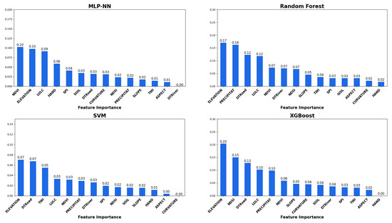
Figure 8.
Feature importance of each machine learning model.
3.3. Model Validation
Model performance was evaluated using several indicators, including sensitivity, specificity, positive predictive value (PPV), negative predictive value (NPV), and AUC, on both the training and test datasets to assess predictive reliability, as shown in Table 9. Among the four algorithms, XGBoost demonstrated the best performance, with the highest AUC (0.9291), sensitivity (0.8824), and specificity (0.8718) on the test data, indicating superior accuracy in detecting flood-prone areas. Random Forest model also performed well, with an AUC of 0.9286, a sensitivity of 0.8039, and a specificity of 0.8718, showing good but slightly lower stability than XGBoost. SVM achieved moderate results, with a sensitivity of 0.7451, a specificity of 0.8718, and an AUC of 0.9236, while MLP-NN had the lowest performance with a sensitivity of 0.7843, a specificity of 0.8718, and an AUC of 0.9105.
Table 9.
Evaluation of sensitivity, specificity, and predictive performance of ML models.
The ROC curve (Figure 9) shows the performance curve of each model based on the relationship between the true positive rate (sensitivity) and false positive rate (specificity). From the graph, XGBoost shows the ROC curve closest to the upper left corner, with an AUC value of 0.9291, slightly outperforming Random Forest (0.9286), SVM (0.9236), and MLP-NN (0.9105). Further evaluation of the model’s classification performance, as shown in Table 10, confirmed the strong discriminative power of XGBoost in distinguishing between flood- and non-flood-prone areas, with XGBoost having a standard error of 0.0121 and a 95% confidence interval from 0.9054 to 0.9528, Random Forest having a standard error of 0.0121 and a confidence interval from 0.9048 to 0.9524, SVM having a standard error of 0.0125 and a confidence interval from 0.899 to 0.9481, and MLP-NN having a standard error of 0.0135 with a confidence interval from 0.8841 to 0.9369.
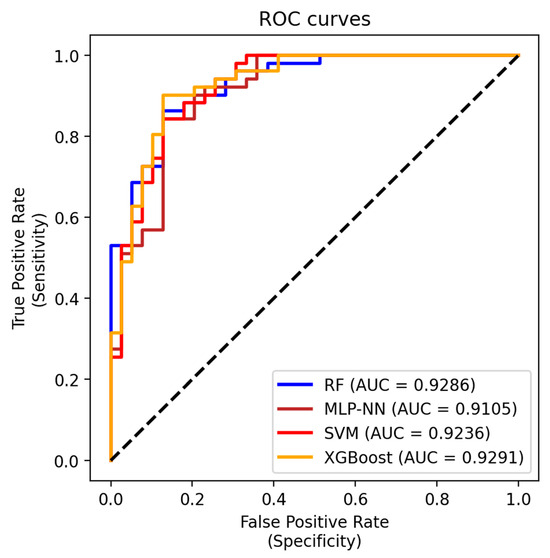
Figure 9.
Model performance based on ROC curves and AUC values for flood susceptibility.
Table 10.
AUROC and 95% confidence interval analysis of machine learning models for flood susceptibility.
Considering all these evaluation metrics, XGBoost emerged as the most optimal model, offering a strong balance across all evaluation metrics for flood susceptibility prediction in the study area. The model recorded the highest accuracy (87.8%), precision (90.0%), recall (88.2%), and F1 score (89.1%), which were consistently better than those of the other models, as shown in Table 11. Its Cohen’s Kappa value of 0.752 indicates an excellent level of predictive agreement between the model’s predictions and the actual data. Therefore, XGBoost can be concluded as the most optimized algorithm for flood susceptibility modeling in the study area.
Table 11.
Comparison of classification performance metrics for flood susceptibility.
3.4. Flood Susceptibility Map
Figure 10 presents flood susceptibility maps generated with MLP-NN, Random Forest, SVM, and XGBoost. All models consistently identified high to very high susceptibility class, mainly concentrated in the central and southeastern areas of Demak District. We classified flood susceptibility into five categories (very low, low, moderate, high, and very high) using the natural breaks (Jenks) classification method. However, classification sharpness varied across models. XGBoost demonstrated the most structured and distinct segmentation, especially in the northern region, where it classified some areas as low susceptibility, contrasting with other models indicating superior sensitivity to local hydrological and topographical variations. Random Forest also showed detailed classifications but tended to over-predict medium susceptibility class. SVM and MLP-NN maps exhibited more scattered high-susceptibility classes and lower classification clarity. Based on these results, the XGBoost model produced the most accurate and spatially coherent flood susceptibility maps. A subsequent analysis of the proportion of susceptibility classes further assessed each model’s ability to distinguish between risk levels and identify the most balanced classification.
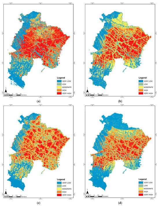
Figure 10.
Spatial distribution of susceptibility maps generated via (a) MLP-NN, (b) Random Forest (c) SVM, and (d) XGBoost.
Figure 11 shows the percentage distribution of areas by flood susceptibility class as predicted by four machine learning models. The XGBoost model produced a relatively balanced classification, assigning 36.60% of the area to the very low category and 16.67% to the very high category, suggesting a conservative tendency in identifying high-risk zones. In contrast, the MLP-NN model classified 34.12% of areas as very low and the highest proportion (29.83%) as very high, indicating a possible overestimation of flood-prone regions. Random Forest and SVM showed similar trends, with very high classifications at 22.64% and 20.86%, respectively. These results suggest that while all models capture the spatial distribution of risk, XGBoost stands out by delivering more balanced and realistic flood susceptibility predictions. Based on the visual overlay between the flood susceptibility modeling results and the sample points (Figure 12), the XGBoost model shows the highest spatial match between the high-susceptibility areas and the locations of the flood points (red triangles) and between the low-susceptibility areas and the locations of non-flood points (blue triangles), particularly in the northern Demak District. This finding is in line with the previous quantitative evaluation results, where XGBoost obtained the highest AUC of 0.9291 and a classification accuracy of 87.8% (Table 9 and Table 11).
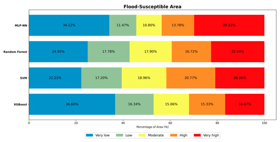
Figure 11.
Percentage of flood susceptibility area.
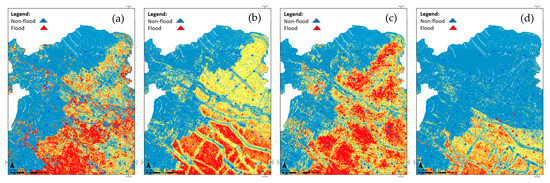
Figure 12.
Visual validation of flood susceptibility maps generated with four machine learning models using flood and non-flood sample points: (a) MLP-NN, (b) Random Forest, (c) SVM, and (d) XGBoost.
Table 12 explains the flood susceptibility area distribution across five classes for each model. XGBoost estimated the largest very low area (343.36 km2) and the smallest very high area (156.35 km2), indicating a tendency toward a conservative classification of high-risk zones. MLP-NN predicted the highest very high area (276.12 km2), suggesting possible overestimation of risk. Random Forest and SVM showed more moderate patterns but still allocated substantial areas to the high-risk categories.
Table 12.
Flood susceptibility area distribution (km2) predicted by MLP-NN, Random Forest, SVM, and XGBoost.
3.5. Feature Contribution
To interpret the machine learning model and understand the quantitative contribution of each factor to the prediction of flood susceptibility, we employed the SHAP (SHapley Additive exPlanations) method. The results of the SHAP analysis, summarized in Figure 13, present a clear hierarchy of feature importance and the direction of their respective impacts.
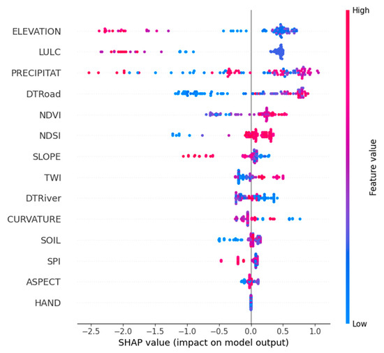
Figure 13.
SHAP (SHapley Additive exPlanations) summary plot for the XGBoost model, showing the contribution of each flood conditioning factor.
The SHAP analysis reveals how a combination of physical and land cover factors drives flood susceptibility. Physically, elevation is the key determinant, with lowlands being the most at-risk zones; this is exacerbated by high precipitation, which acts as a primary trigger. Regarding land cover, areas with high vegetation density (NDVI) and those dominated by cropland (LULC) exhibit greater vulnerability. This effect is amplified by anthropogenic factors such as proximity to roads (DTRoad), which often alters natural drainage and increases surface runoff. This is consistent with the visual map shown in Figure 10, where most of the flood-prone areas are located in cropland areas, which can lead to crop failure.
The SHAP analysis further reveals the significant influence of key topographical and hydrological factors. Specifically, high Topographic Wetness Index (TWI) values, which signify water accumulation, are shown to consistently increase flood susceptibility. Furthermore, land curvature is found to modulate surface water flow patterns, while proximity to rivers (DTRiver) inherently elevates flood risk. The SHAP results underscore the critical importance of these complex interactions among topographical and hydrological variables for accurate flood susceptibility modeling.
3.6. Future Flood Projection
Following the successful development of the current flood susceptibility model, the subsequent phase focuses on projecting future flood susceptibility. This projection is based on three Shared Socioeconomic Pathway (SSP) scenarios, SSP1-2.6, SSP2-4.5, and SSP5-8.5, derived from the Coupled Model Intercomparison Project Phase 6 (CMIP6) Global Climate Models (GCMs). XGBoost was selected for future flood projections due to its superior performance and optimal results demonstrated in previous model evaluations.
3.6.1. Multi-Model Ensemble
Model performance was evaluated using observed data from three gauges station—Brumbung, Bungo, and Jatisono as presented in Table 13. The results show a strong agreement between the simulated and observed data, with correlation coefficients (r) ranging from 0.98 to 0.99 and Nash–Sutcliffe Efficiency (NSE) values between 0.80 and 0.92. The RMSE values remain relatively low (31.1 to 55.63), while the index of agreement (md) is close to 1.0 across all stations, indicating minimal systematic bias. The agreement between observed and ensemble-simulated monthly precipitation at the three stations is further illustrated in Figure 14, demonstrating the model’s ability to replicate temporal precipitation patterns across the historical period, with some minor discrepancies in peak precipitation years. Ensembles of climate models are important because they improve the accuracy of climate change projections and help quantify climate uncertainty associated with individual model projections. These findings further confirm the reliability and suitability of the ensemble model for projecting future flood susceptibility under various climate scenarios.
Table 13.
Multi-model ensemble performance metrics.
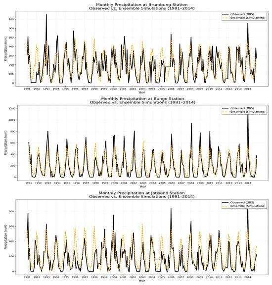
Figure 14.
Observed against ensemble monthly precipitation in Brumbung, Bungo, and Jatisono.
3.6.2. Future Flood Projection in Different Scenarios
To assess the potential impact of climate change on future flood susceptibility, flood projections were made for the Demak District under three distinct climate scenarios: SSP1-2.6, SSP2-4.5, and SSP5-8.5. These scenarios represent various pathways of socioeconomic development and greenhouse gas emissions, ranging from low to high emissions. The projections utilized the precipitation data derived from the multi-model ensemble of CMIP6 GCM, which was processed earlier in this study, to model future flood susceptibility from 2021 to 2100.
The spatial distribution of MME precipitation, as shown in Figure 15, illustrates the projected changes in precipitation under different climate scenarios (SSP1-2.6, SSP2-4.5, and SSP5-8.5) from 2021 to 2100. The multi-model ensemble projections reveal an increase in precipitation across all scenarios, with the highest increases observed under the SSP5-8.5 scenario. Notably, the highest precipitation is projected to be concentrated in the northern region of Demak, which borders the Java Sea. Table 14 provides supporting statistical data on maximum, minimum, and average precipitation for each period under the different scenarios, reinforcing the conclusion that rising emissions will lead to more extreme precipitation events.
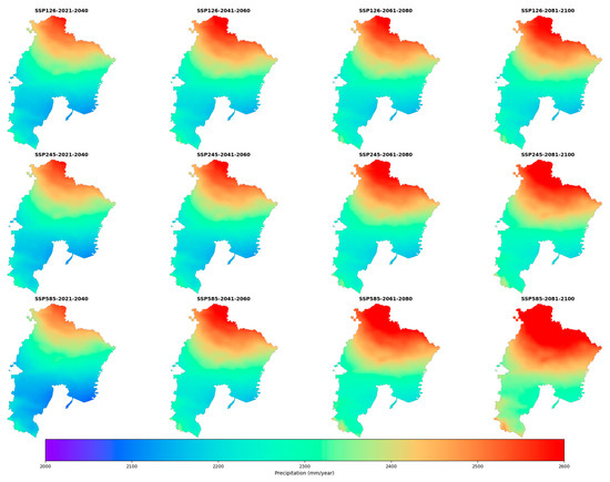
Figure 15.
Multi-model ensemble (MME) projected precipitation under different scenarios.
Table 14.
Maximum, minimum, and average precipitation in different scenarios.
Figure 16 depicts the spatial distribution of flood susceptibility maps for Demak District based on climate change projections under three Shared Socioeconomic Pathway (SSP) scenarios (SSP1-2.6, SSP2-4.5, and SSP5-8.5) from 2021 to 2100. Each scenario is divided into four time periods: 2021–2040, 2041–2060, 2061–2080, and 2081–2100. The maps depict variations in flood susceptibility based on projected precipitation increases, with areas of higher susceptibility indicated by red and areas of lower susceptibility shown in blue. The SSP1-2.6 scenario, representing a low-emission pathway, shows relatively fewer areas in the high- and very-high-susceptibility classes compared to those in the SSP2-4.5 and SSP5-8.5 scenarios, which, under higher-emission pathways, exhibit an expansion in these high-susceptibility zones. This indicates that as emissions increase, flood susceptibility is projected to rise. These maps provide an overview of how flood risks in Demak may increase over time, driven by escalating greenhouse gas emissions.
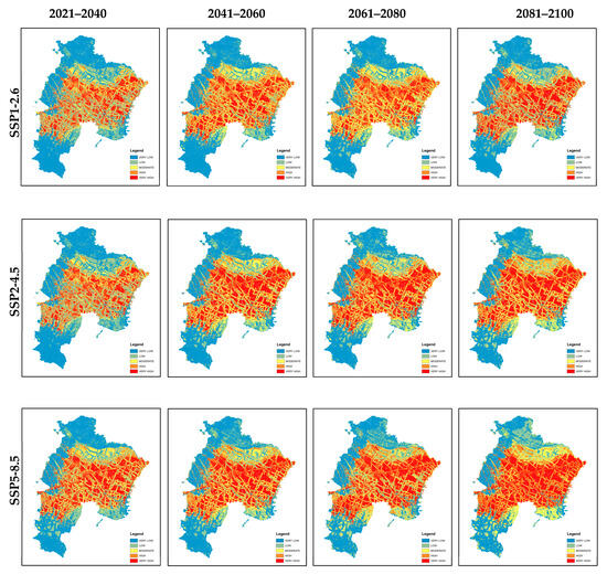
Figure 16.
Spatial distribution of flood susceptibility maps in different scenarios and periods.
Figure 17 and Table 15, Table 16 and Table 17 illustrate the projected changes in flood susceptibility for Demak District under climate change scenarios SSP1-2.6, SSP2-4.5, and SSP5-8.5 from 2021 to 2100. The projections show that as greenhouse gas emissions increase, areas with very high flood susceptibility are expected to rise significantly. Under the SSP1-2.6 scenario (low emission pathway), areas with very low flood susceptibility remain relatively stable, decreasing slightly from 36.6% in the current period to 31.64% in 2081–2100. However, under the SSP5-8.5 scenario (high emission pathway), areas with very high flood susceptibility are projected to increase sharply from 16.67% to 27.43%, indicating a growing flood susceptibility. Table 13, Table 14 and Table 15 provide detailed changes in flood susceptibility area distribution for each scenario and period, highlighting that under high-emission scenarios (SSP5-8.5), the expansion of very-high-susceptibility areas is more pronounced compared with that of low-emission scenarios (SSP1-2.6), with the most dramatic changes occurring in the period of 2081–2100.
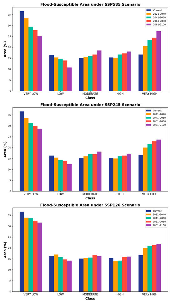
Figure 17.
Bar charts showing the percentage of flood susceptible areas under different climate scenarios (SSP1-2.6, SSP2-4.5, and SSP5-8.5) for the periods 2021–2040, 2041–2060, 2061–2080, and 2081–2100, along with the current (baseline) condition.
Table 15.
Flood susceptibility area (%) under SSP1-2.6 compared with current flood susceptibility.
Table 16.
Flood susceptibility area (%) under SSP2-4.5 compared with current flood susceptibility.
Table 17.
Flood susceptibility area (%) under SSP5-8.5 compared with current flood susceptibility.
Table 18 and Table 19 further analyze the risk trend percentage changes in flood susceptibility areas across the different scenarios. Red represents changes that lead to an increase in susceptibility (i.e., positive changes), while blue indicates changes that result in a decrease in susceptibility (i.e., negative changes). These tables highlight significant differences between the various periods within each scenario. Under SSP1-2.6, very-low-susceptibility areas show a slight reduction, but the very-high-susceptibility areas increase gradually. In contrast, under SSP2-4.5 and SSP5-8.5, the increase in very-high-risk areas is much more significant, with SSP5-8.5 showing the largest increase across all periods. The very low and low areas show a downward trend of change throughout the period and all scenarios, while the high and very high areas show an upward trend. The largest difference in change occurred in the period 2081–2100 in SSP585-SSP245, by about 3.81%. Although fluctuations in change are seen, this underscores the severe impact of climate change on flood susceptibility, especially in regions such as Demak District, which is expected to face escalating flood risks over time.
Table 18.
Percentages of changes in flood susceptibility area (%) over four periods in each scenario.
Table 19.
Percentages of changes in flood susceptibility area (%) based on changes in climate change scenario for each period.
To summarize the long-term impacts, Table 20 condenses the projected changes in the ‘Very High’ flood susceptibility area. The results clearly show a significant expansion of this high-risk zone by the end of the century across all scenarios, with the most severe increase occurring under the high-emission SSP5-8.5 pathway. The projected expansion of ‘Very High’ flood susceptibility class (from 16.67% to over 27% under SSP5-8.5) demands urgent action. These findings provide a critical evidence base for local stakeholders to revise spatial planning policies, upgrade infrastructure, and expand community preparedness programs to adapt to the escalating future flood risk.
Table 20.
Summary of projected changes in very high flood susceptibility area by 2081–2100.
4. Discussion
Integrating machine learning algorithms with remote sensing data has proven to be an effective approach for generating an accurate flood susceptibility model. In this study, we applied machine learning techniques such as Random Forest, MLP-NN, SVM, and XGBoost to model current and future flood susceptibility in Demak District, Indonesia. The models performed well in identifying areas with varying levels of flood susceptibility, with XGBoost emerging as the most effective model due to its high accuracy and ability to clearly distinguish between different susceptibility classes. XGBoost excels because of its ability to reduce overfitting, handle complex non-linear relationships between variables, and efficiently process large datasets, making it particularly suited for the complex environmental factors affecting flood susceptibility in Demak [83]. Environmental factors such as elevation, precipitation, and land use showed strong correlations with flood susceptibility, which aligns with findings from previous studies that emphasize the importance of topographic and hydrological variables in determining flood-prone areas, particularly in low-lying regions such as Demak [84,85,86].
The projections based on different Shared Socioeconomic Pathway (SSP) scenarios (SSP1-2.6, SSP2-4.5, SSP5-8.5) highlight the significant impact of increased greenhouse gas emissions on flood susceptibility. This is directly related to the intensification of precipitation patterns triggered by global warming: high-emission scenarios (SSP5-8.5) lead to more intense evaporation and a more active hydrological cycle, which result in increased extreme precipitation and higher intensity precipitation events. Under the SSP5-8.5 scenario, areas with very high flood susceptibility are projected to rise from 16.67% (current period) to 27.43% (2081–2100). In contrast, the increase in very high susceptibility areas under the SSP1-2.6 scenario is much more moderate. This demonstrates that higher emission pathways not only raise global temperatures but also drive changes in precipitation patterns, leading to more frequent and intense extreme precipitation, which directly increases flood susceptibility.
Although the projected flood susceptibility shows a generally increasing trend across future time periods, this is a direct response to the consistent rise in precipitation projected by CMIP6 GCMs. It is important to note that this finding operates under the explicit limitation and assumption that non-climatic factors, such as land use and infrastructure, remain unchanged. Moreover, despite resampling the GCM data for spatial consistency, inherent uncertainties associated with the climate models and the future projection scenarios themselves persist and impact the final susceptibility outputs.
The utilization of Sentinel-1 SAR imagery for flood inventory mapping proved invaluable, especially considering the challenges posed by limited field data in Demak. SAR’s ability to detect flooded areas regardless of cloud cover enabled the development of accurate flood inventory maps [87]. These maps, including those for the severe flood event in March 2024, provide reliable data for training machine learning models, which improves the spatial accuracy of flood susceptibility models. While our use of Sentinel-1 SAR imagery provided a robust flood inventory, we acknowledge a limitation in its validation. The process relied on comparison with UNOSAT data, another satellite product, as direct field surveys were not feasible for such a large-scale event due to logistical constraints. Despite this, validating against a reputable, independent dataset was the most robust alternative, and the high accuracy achieved (>89.00%) supports the reliability of our flood inventory for model training. The absence of ground-truth data is a limitation that future studies could address.
The multi-model ensemble approach for future projections also enhances the reliability of the results by reducing uncertainty [88,89]. Through the selection of the highest-ranking CMIP6 GCMs using the Rating Metric as a basis, we achieved more consistent precipitation projections, which strengthens the flood susceptibility model. A limitation of this validation is the reliance on only three-gauge stations for a large 995.32 km2 area. However, these were the only official stations with reliable, long-term data available from BMKG. Despite this low spatial density, the strong performance of the ensemble model at these locations provides confidence in its predictive capabilities.
This study highlights that future flood susceptibility is influenced not only by changes in precipitation patterns due to emissions but also by local environmental factors. Firstly, future research should explore the integration of socioeconomic data (population density) and land use land cover (LULC) prediction into flood susceptibility models to create more context-specific and actionable maps. Since LULC significantly influences flood susceptibility, methods such as CA-MARKOV or CA-ANN for LULC prediction could enhance the accuracy of these models [90,91], and also incorporate temporal analysis. Secondly, while this study provides a static susceptibility map, a significant future step would be to couple this model with real-time precipitation data and satellite imagery to develop an operational flood early warning system. This would transition the research from a planning tool to an active disaster management solution, providing timely alerts to vulnerable communities, ultimately supporting more effective flood risk management and adaptation planning.
5. Conclusions
This study successfully developed novel integration of Sentinel-1 SAR, remote sensing, CMIP6 GCM data, and machine learning techniques to robustly predict current and future flood susceptibility models in Demak District. The XGBoost model demonstrated the highest accuracy in identifying flood-prone areas, providing a clear spatial representation of flood susceptibility. XGBoost’s ability to reduce overfitting, handle complex non-linear relationships between variables, and process large datasets efficiently made it particularly effective for this analysis. Remote sensing data, particularly Sentinel-1 SAR, have proven invaluable for generating flood inventories and improving the accuracy of susceptibility models in the absence of extensive field data.
Projections using CMIP6 GCM precipitation data under different climate change scenarios (SSP1-2.6, SSP2-4.5, and SSP5-8.5) indicate a significant increase in flood susceptibility in Demak District, especially under higher emission scenarios. The area of very high flood susceptibility is projected to grow notably by the end of the century, emphasizing the increasing impact of climate change on flood susceptibility in the region.
The integration of climate projections into flood susceptibility modeling provides valuable insights into how flood susceptibility will evolve over time due to changing precipitation patterns and greenhouse gas emissions. These findings underline the urgent need for sustainable adaptive flood management strategies to address the growing flood susceptibility in Demak, especially in the context of climate change and rising emissions.
Author Contributions
Conceptualization, T.-H.L.; methodology, A.V., F.T. and T.-H.L.; software, A.V. and Y.-L.C.; validation, A.V.; formal analysis and investigation, T.-H.L. and A.V.; data curation, A.V. and F.-C.W.; writing—original draft preparation, A.V. and T.-H.L.; writing—review and editing, T.-H.L., F.T. and A.V.; supervision, project administration, and funding acquisition, T.-H.L. All authors have read and agreed to the published version of the manuscript.
Funding
This work was financially supported by the Taiwan National Science and Technology Council (NSTC), grant NSTC 113-2119-M-008-014 and NSTC 113-2111-M-008-029.
Institutional Review Board Statement
Not applicable.
Informed Consent Statement
Not applicable.
Data Availability Statement
The data that supports the findings of this study are available from the corresponding author upon reasonable request.
Conflicts of Interest
The authors declare no conflicts of interest.
References
- Shen, G.; Hwang, S.N. Spatial–Temporal Snapshots of Global Natural Disaster Impacts Revealed from EM-DAT for 1900–2015. Geomat. Nat. Hazards Risk 2019, 10, 912–934. [Google Scholar] [CrossRef]
- Bui, D.T.; Tsangaratos, P.; Ngo, P.T.T.; Pham, T.D.; Pham, B.T. Flash Flood Susceptibility Modeling Using an Optimized Fuzzy Rule Based Feature Selection Technique and Tree Based Ensemble Methods. Sci. Total Environ. 2019, 668, 1038–1054. [Google Scholar] [CrossRef] [PubMed]
- Chowdhuri, I.; Pal, S.C.; Chakrabortty, R. Flood Susceptibility Mapping by Ensemble Evidential Belief Function and Binomial Logistic Regression Model on River Basin of Eastern India. Adv. Space Res. 2020, 65, 1466–1489. [Google Scholar] [CrossRef]
- Gai, L.; Nunes, J.P.; Baartman, J.E.M.; Zhang, H.; Wang, F.; de Roo, A.; Ritsema, C.J.; Geissen, V. Assessing the Impact of Human Interventions on Floods and Low Flows in the Wei River Basin in China Using the LISFLOOD Model. Sci. Total Environ. 2019, 653, 1077–1094. [Google Scholar] [CrossRef]
- Gholami, F.; Sedighifar, Z.; Ghaforpur, P.; Li, Y.; Zhang, J. Spatial–Temporal Analysis of Various Land Use Classifications and Their Long-Term Alteration’s Impact on Hydrological Components: Using Remote Sensing, SAGA-GIS, and ARCSWAT Model. Environ. Sci. Water Res. Technol. 2023, 9, 1161–1181. [Google Scholar] [CrossRef]
- Roy, P.; Chandra Pal, S.; Chakrabortty, R.; Chowdhuri, I.; Malik, S.; Das, B. Threats of Climate and Land Use Change on Future Flood Susceptibility. J. Clean. Prod. 2020, 272, 122757. [Google Scholar] [CrossRef]
- Filonchyk, M.; Peterson, M.P.; Zhang, L.; Hurynovich, V.; He, Y. Greenhouse Gases Emissions and Global Climate Change: Examining the Influence of CO2, CH4, and N2O. Sci. Total Environ. 2024, 935, 173359. [Google Scholar] [CrossRef]
- Prăvălie, R.; Bandoc, G.; Patriche, C.; Sternberg, T. Recent Changes in Global Drylands: Evidences from Two Major Aridity Databases. Catena 2019, 178, 209–231. [Google Scholar] [CrossRef]
- Kim, J.C.; Lee, S.; Jung, H.S.; Lee, S. Landslide Susceptibility Mapping Using Random Forest and Boosted Tree Models in Pyeong-Chang, Korea. Geocarto Int. 2018, 33, 1000–1015. [Google Scholar] [CrossRef]
- Coronese, M.; Lamperti, F.; Keller, K.; Chiaromonte, F.; Roventini, A. Evidence for Sharp Increase in the Economic Damages of Extreme Natural Disasters. Proc. Natl. Acad. Sci. USA 2019, 116, 21450–21455. [Google Scholar] [CrossRef]
- Rajkhowa, S.; Sarma, J. Climate Change and Flood Risk, Global Climate Change. Glob. Clim. Change 2021, 321–339. [Google Scholar] [CrossRef]
- Janizadeh, S.; Kim, D.; Jun, C.; Bateni, S.M.; Pandey, M.; Mishra, V.N. Impact of Climate Change on Future Flood Susceptibility Projections under Shared Socioeconomic Pathway Scenarios in South Asia Using Artificial Intelligence Algorithms. J. Environ. Manag. 2024, 366, 121764. [Google Scholar] [CrossRef]
- Mahdian, M.; Hosseinzadeh, M.; Siadatmousavi, S.M.; Chalipa, Z.; Delavar, M.; Guo, M.; Abolfathi, S.; Noori, R. Modelling Impacts of Climate Change and Anthropogenic Activities on Inflows and Sediment Loads of Wetlands: Case Study of the Anzali Wetland. Sci. Rep. 2023, 13, 5399. [Google Scholar] [CrossRef]
- Kurniadi, A.; Weller, E.; Kim, Y.H.; Min, S.K. Evaluation of Coupled Model Intercomparison Project Phase 6 Model-Simulated Extreme Precipitation over Indonesia. Int. J. Climatol. 2023, 43, 174–196. [Google Scholar] [CrossRef]
- Ge, F.; Zhu, S.; Luo, H.; Zhi, X.; Wang, H. Future Changes in Precipitation Extremes over Southeast Asia: Insights from CMIP6 Multi-Model Ensemble. Environ. Res. Lett. 2021, 16, 024013. [Google Scholar] [CrossRef]
- Eyring, V.; Bony, S.; Meehl, G.A.; Senior, C.A.; Stevens, B.; Stouffer, R.J.; Taylor, K.E. Overview of the Coupled Model Intercomparison Project Phase 6 (CMIP6) Experimental Design and Organization. Geosci. Model. Dev. 2016, 9, 1937–1958. [Google Scholar] [CrossRef]
- O’Neill, B.C.; Tebaldi, C.; Van Vuuren, D.P.; Eyring, V.; Friedlingstein, P.; Hurtt, G.; Knutti, R.; Kriegler, E.; Lamarque, J.F.; Lowe, J.; et al. The Scenario Model Intercomparison Project (ScenarioMIP) for CMIP6. Geosci. Model. Dev. 2016, 9, 3461–3482. [Google Scholar] [CrossRef]
- Aryal, A.; Acharya, A.; Kalra, A. Assessing the Implication of Climate Change to Forecast Future Flood Using CMIP6 Climate Projections and HEC-RAS Modeling. Forecasting 2022, 4, 582–603. [Google Scholar] [CrossRef]
- Sun, J.; Yan, H.; Bao, Z.; Wang, G. Investigating Impacts of Climate Change on Runoff from the Qinhuai River by Using the SWAT Model and CMIP6 Scenarios. Water 2022, 14, 1778. [Google Scholar] [CrossRef]
- Mia, M.U.; Chowdhury, T.N.; Chakrabortty, R.; Pal, S.C.; Al-Sadoon, M.K.; Costache, R.; Islam, A.R.M.T. Flood Susceptibility Modeling Using an Advanced Deep Learning-Based Iterative Classifier Optimizer. Land 2023, 12, 810. [Google Scholar] [CrossRef]
- Liu, J.; Wang, J.; Xiong, J.; Cheng, W.; Li, Y.; Cao, Y.; He, Y.; Duan, Y.; He, W.; Yang, G. Assessment of Flood Susceptibility Mapping Using Support Vector Machine, Logistic Regression and Their Ensemble Techniques in the Belt and Road Region. Geocarto Int. 2022, 37, 9817–9846. [Google Scholar] [CrossRef]
- Shahabi, H.; Shirzadi, A.; Ghaderi, K.; Omidvar, E.; Al-Ansari, N.; Clague, J.J.; Geertsema, M.; Khosravi, K.; Amini, A.; Bahrami, S.; et al. Flood Detection and Susceptibility Mapping Using Sentinel-1 Remote Sensing Data and a Machine Learning Approach: Hybrid Intelligence of Bagging Ensemble Based on K-Nearest Neighbor Classifier. Remote Sens. 2020, 12, 266. [Google Scholar] [CrossRef]
- de Brito, M.M.; Almoradie, A.; Evers, M. Spatially-Explicit Sensitivity and Uncertainty Analysis in a MCDA-Based Flood Vulnerability Model. Int. J. Geogr. Inf. Sci. 2019, 33, 1788–1806. [Google Scholar] [CrossRef]
- Ranjgar, B.; Razavi-Termeh, S.V.; Foroughnia, F.; Sadeghi-Niaraki, A.; Perissin, D. Land Subsidence Susceptibility Mapping Using Persistent Scatterer SAR Interferometry Technique and Optimized Hybrid Machine Learning Algorithms. Remote Sens. 2021, 13, 1326. [Google Scholar] [CrossRef]
- Dodangeh, E.; Singh, V.P.; Pham, B.T.; Yin, J.; Yang, G.; Mosavi, A. Flood Frequency Analysis of Interconnected Rivers by Copulas. Water Resour. Manag. 2020, 34, 3533–3549. [Google Scholar] [CrossRef]
- Mishra, A.; Mukherjee, S.; Merz, B.; Singh, V.P.; Wright, D.B.; Villarini, G.; Paul, S.; Kumar, D.N.; Khedun, C.P.; Niyogi, D.; et al. An Overview of Flood Concepts, Challenges, and Future Directions. J. Hydrol. Eng. 2022, 27, 03122001. [Google Scholar] [CrossRef]
- Samanta, S.; Pal, D.K.; Palsamanta, B. Flood Susceptibility Analysis through Remote Sensing, GIS and Frequency Ratio Model. Appl. Water Sci. 2018, 8, 66. [Google Scholar] [CrossRef]
- Tehrany, M.S.; Pradhan, B.; Jebur, M.N. Flood Susceptibility Mapping Using a Novel Ensemble Weights-of-Evidence and Support Vector Machine Models in GIS. J. Hydrol. 2014, 512, 332–343. [Google Scholar] [CrossRef]
- Mehravar, S.; Razavi-Termeh, S.V.; Moghimi, A.; Ranjgar, B.; Foroughnia, F.; Amani, M. Flood Susceptibility Mapping Using Multi-Temporal SAR Imagery and Novel Integration of Nature-Inspired Algorithms into Support Vector Regression. J. Hydrol. 2023, 617, 129100. [Google Scholar] [CrossRef]
- Ngo, P.T.T.; Pham, T.D.; Nhu, V.H.; Le, T.T.; Tran, D.A.; Phan, D.C.; Hoa, P.V.; Amaro-Mellado, J.L.; Bui, D.T. A Novel Hybrid Quantum-PSO and Credal Decision Tree Ensemble for Tropical Cyclone Induced Flash Flood Susceptibility Mapping with Geospatial Data. J. Hydrol. 2021, 596, 125682. [Google Scholar] [CrossRef]
- Beck, H.E.; Zimmermann, N.E.; McVicar, T.R.; Vergopolan, N.; Berg, A.; Wood, E.F. Present and Future Köppen-Geiger Climate Classification Maps at 1-Km Resolution. Sci. Data 2018, 5, 180214. [Google Scholar] [CrossRef]
- Benzougagh, B.; Frison, P.L.; Meshram, S.G.; Boudad, L.; Dridri, A.; Sadkaoui, D.; Mimich, K.; Khedher, K.M. Flood Mapping Using Multi-Temporal Sentinel-1 SAR Images: A Case Study—Inaouene Watershed from Northeast of Morocco. Iran. J. Sci. Technol. Trans. Civ. Eng. 2022, 46, 1481–1490. [Google Scholar] [CrossRef]
- Moharrami, M.; Javanbakht, M.; Attarchi, S. Automatic Flood Detection Using Sentinel-1 Images on the Google Earth Engine. Environ. Monit. Assess. 2021, 193, 248. [Google Scholar] [CrossRef] [PubMed]
- Pelich, R.-M.; Schumann, G.; Giustarini, L.; Tran, K.H.; Menenti, M.; Jia, L. Surface Water Mapping and Flood Monitoring in the Mekong Delta Using Sentinel-1 SAR Time Series and Otsu Threshold. Remote Sens. 2022, 14, 5721. [Google Scholar] [CrossRef]
- Tiwari, V.; Kumar, V.; Matin, M.A.; Thapa, A.; Ellenburg, W.L.; Gupta, N.; Thapa, S. Flood Inundation Mapping-Kerala 2018; Harnessing the Power of SAR, Automatic Threshold Detection Method and Google Earth Engine. PLoS ONE 2020, 15, e0237324. [Google Scholar] [CrossRef]
- Ahmad, A.; Chen, J.; Chen, X.; Khadka, N.; Khan, M.U.; Wang, C.; Tayyab, M. Flood Risk Modelling by the Synergistic Approach of Machine Learning and Best-Worst Method in Indus Kohistan, Western Himalaya. Geomat. Nat. Hazards Risk 2025, 16, 2469766. [Google Scholar] [CrossRef]
- Kia, M.B.; Pirasteh, S.; Pradhan, B.; Mahmud, A.R.; Sulaiman, W.N.A.; Moradi, A. An Artificial Neural Network Model for Flood Simulation Using GIS: Johor River Basin, Malaysia. Environ. Earth Sci. 2012, 67, 251–264. [Google Scholar] [CrossRef]
- Karpouza, M.; Bathrellos, G.D.; Kaviris, G.; Antonarakou, A.; Skilodimou, H.D. How Could Students Be Safe during Flood and Tsunami Events? Int. J. Disaster Risk Reduct. 2023, 95, 103830. [Google Scholar] [CrossRef]
- Khosravi, K.; Pourghasemi, H.R.; Chapi, K.; Bahri, M. Flash Flood Susceptibility Analysis and Its Mapping Using Different Bivariate Models in Iran: A Comparison between Shannon’s Entropy, Statistical Index, and Weighting Factor Models. Environ. Monit. Assess. 2016, 188, 656. [Google Scholar] [CrossRef]
- Pham, B.T.; Luu, C.; Van Phong, T.; Nguyen, H.D.; Van Le, H.; Tran, T.Q.; Ta, H.T.; Prakash, I. Flood Risk Assessment Using Hybrid Artificial Intelligence Models Integrated with Multi-Criteria Decision Analysis in Quang Nam Province, Vietnam. J. Hydrol. 2021, 592, 125815. [Google Scholar] [CrossRef]
- Choubin, B.; Moradi, E.; Golshan, M.; Adamowski, J.; Sajedi-Hosseini, F.; Mosavi, A. An Ensemble Prediction of Flood Susceptibility Using Multivariate Discriminant Analysis, Classification and Regression Trees, and Support Vector Machines. Sci. Total Environ. 2019, 651, 2087–2096. [Google Scholar] [CrossRef]
- Kazakis, N.; Kougias, I.; Patsialis, T. Assessment of Flood Hazard Areas at a Regional Scale Using an Index-Based Approach and Analytical Hierarchy Process: Application in Rhodope-Evros Region, Greece. Sci. Total Environ. 2015, 538, 555–563. [Google Scholar] [CrossRef]
- Chen, Y.; Liu, R.; Barrett, D.; Gao, L.; Zhou, M.; Renzullo, L.; Emelyanova, I. A Spatial Assessment Framework for Evaluating Flood Risk under Extreme Climates. Sci. Total Environ. 2015, 538, 512–523. [Google Scholar] [CrossRef] [PubMed]
- Rahmati, O.; Hamid Reza, P.; Zeinivand, H. Flood Susceptibility Mapping Using Frequency Ratio and Weights-of-Evidence Models in the Golastan Province, Iran. Geocarto Int. 2016, 31, 42–70. [Google Scholar] [CrossRef]
- Regmi, A.D.; Devkota, K.C.; Yoshida, K.; Pradhan, B.; Pourghasemi, H.R.; Kumamoto, T.; Akgun, A. Application of Frequency Ratio, Statistical Index, and Weights-of-Evidence Models and Their Comparison in Landslide Susceptibility Mapping in Central Nepal Himalaya. Arab. J. Geosci. 2014, 7, 725–742. [Google Scholar] [CrossRef]
- Mohammadi, A.; Kamran, K.V.; Karimzadeh, S.; Shahabi, H.; Al-Ansari, N. Flood Detection and Susceptibility Mapping Using Sentinel-1 Time Series, Alternating Decision Trees, and Bag-ADTree Models. Complexity 2020, 2020, 4271376. [Google Scholar] [CrossRef]
- Fiorentino, C.; Donvito, A.R.; D’Antonio, P.; Lopinto, S. Experimental Methodology for Prescription Maps of Variable Rate Nitrogenous Fertilizers on Cereal Crops. In Innovative Biosystems Engineering for Sustainable Agriculture, Forestry and Food Production; Springer: Cham, Switzerland, 2020; Volume 67, pp. 863–872. [Google Scholar] [CrossRef]
- Aalto, R.; Maurice-Bourgoin, L.; Dunne, T.; Montgomery, D.R.; Nittrouer, C.A.; Guyot, J.L. Episodic Sediment Accumulation on Amazonian Flood Plains Influenced by El Niño/Southern Oscillation. Nature 2003, 425, 493–497. [Google Scholar] [CrossRef]
- Khosravi, K.; Shahabi, H.; Pham, B.T.; Adamowski, J.; Shirzadi, A.; Pradhan, B.; Dou, J.; Ly, H.B.; Gróf, G.; Ho, H.L.; et al. A Comparative Assessment of Flood Susceptibility Modeling Using Multi-Criteria Decision-Making Analysis and Machine Learning Methods. J. Hydrol. 2019, 573, 311–323. [Google Scholar] [CrossRef]
- Yalcin, A.; Reis, S.; Aydinoglu, A.C.; Yomralioglu, T. A GIS-Based Comparative Study of Frequency Ratio, Analytical Hierarchy Process, Bivariate Statistics and Logistics Regression Methods for Landslide Susceptibility Mapping in Trabzon, NE Turkey. Catena 2011, 85, 274–287. [Google Scholar] [CrossRef]
- Soltani, K.; Ebtehaj, I.; Amiri, A.; Azari, A.; Gharabaghi, B.; Bonakdari, H. Mapping the Spatial and Temporal Variability of Flood Susceptibility Using Remotely Sensed Normalized Difference Vegetation Index and the Forecasted Changes in the Future. Sci. Total Environ. 2021, 770, 145288. [Google Scholar] [CrossRef]
- Shrestha, S.; Dahal, D.; Poudel, B.; Banjara, M.; Kalra, A. Flood Susceptibility Analysis with Integrated Geographic Information System and Analytical Hierarchy Process: A Multi-Criteria Framework for Risk Assessment and Mitigation. Water 2025, 17, 937. [Google Scholar] [CrossRef]
- Hong, H.; Panahi, M.; Shirzadi, A.; Ma, T.; Liu, J.; Zhu, A.X.; Chen, W.; Kougias, I.; Kazakis, N. Flood Susceptibility Assessment in Hengfeng Area Coupling Adaptive Neuro-Fuzzy Inference System with Genetic Algorithm and Differential Evolution. Sci. Total Environ. 2018, 621, 1124–1141. [Google Scholar] [CrossRef]
- Fang, Z.; Wang, Y.; Peng, L.; Hong, H. Predicting Flood Susceptibility Using LSTM Neural Networks. J. Hydrol. 2021, 594, 125734. [Google Scholar] [CrossRef]
- Tariq, A.; Yan, J.; Ghaffar, B.; Qin, S.; Mousa, B.G.; Sharifi, A.; Huq, M.E.; Aslam, M. Flash Flood Susceptibility Assessment and Zonation by Integrating Analytic Hierarchy Process and Frequency Ratio Model with Diverse Spatial Data. Water 2022, 14, 3069. [Google Scholar] [CrossRef]
- Vibhute, A.D.; Dhumal, R.; Nagne, A.; Surase, R.; Varpe, A.; Gaikwad, S.; Kale, K.V.; Mehrotra, S.C. Evaluation of Soil Conditions Using Spectral Indices from Hyperspectral Datasets. In Proceedings of the 2017 2nd International Conference on Man and Machine Interfacing, Bhubaneswar, India, 21–23 December 2017. [Google Scholar] [CrossRef]
- Nobre, A.D.; Cuartas, L.A.; Hodnett, M.; Rennó, C.D.; Rodrigues, G.; Silveira, A.; Waterloo, M.; Saleska, S. Height Above the Nearest Drainage—A Hydrologically Relevant New Terrain Model. J. Hydrol. 2011, 404, 13–29. [Google Scholar] [CrossRef]
- Aristizabal, F.; Salas, F.; Petrochenkov, G.; Grout, T.; Avant, B.; Bates, B.; Spies, R.; Chadwick, N.; Wills, Z.; Judge, J. Extending Height Above Nearest Drainage to Model Multiple Fluvial Sources in Flood Inundation Mapping Applications for the U.S. National Water Model. Water Resour. Res. 2023, 59, e2022WR032039. [Google Scholar] [CrossRef]
- Arora, A.; Arabameri, A.; Pandey, M.; Siddiqui, M.A.; Shukla, U.K.; Bui, D.T.; Mishra, V.N.; Bhardwaj, A. Optimization of State-of-the-Art Fuzzy-Metaheuristic ANFIS-Based Machine Learning Models for Flood Susceptibility Prediction Mapping in the Middle Ganga Plain, India. Sci. Total Environ. 2021, 750, 141565. [Google Scholar] [CrossRef]
- Khodaei, H.; Nasiri Saleh, F.; Nobakht Dalir, A.; Zarei, E. Future Flood Susceptibility Mapping under Climate and Land Use Change. Sci. Rep. 2025, 15, 12394. [Google Scholar] [CrossRef] [PubMed]
- Asghar Rostami, A.; Taghi Sattari, M.; Apaydin, H.; Milewski, A. Modeling Flood Susceptibility Utilizing Advanced Ensemble Machine Learning Techniques in the Marand Plain. Geosciences 2025, 15, 110. [Google Scholar] [CrossRef]
- Darabi, H.; Rahmati, O.; Naghibi, S.A.; Mohammadi, F.; Ahmadisharaf, E.; Kalantari, Z.; Torabi Haghighi, A.; Soleimanpour, S.M.; Tiefenbacher, J.P.; Tien Bui, D. Development of a Novel Hybrid Multi-Boosting Neural Network Model for Spatial Prediction of Urban Flood. Geocarto Int. 2022, 37, 5716–5741. [Google Scholar] [CrossRef]
- Isabona, J.; Imoize, A.L.; Ojo, S.; Karunwi, O.; Kim, Y.; Lee, C.C.; Li, C.T. Development of a Multilayer Perceptron Neural Network for Optimal Predictive Modeling in Urban Microcellular Radio Environments. Appl. Sci. 2022, 12, 5713. [Google Scholar] [CrossRef]
- Chen, W.; Li, Y.; Xue, W.; Shahabi, H.; Li, S.; Hong, H.; Wang, X.; Bian, H.; Zhang, S.; Pradhan, B.; et al. Modeling Flood Susceptibility Using Data-Driven Approaches of Naïve Bayes Tree, Alternating Decision Tree, and Random Forest Methods. Sci. Total Environ. 2020, 701, 134979. [Google Scholar] [CrossRef]
- Tsagkrasoulis, D.; Montana, G. Random Forest Regression for Manifold-Valued Responses. Pattern Recognit. Lett. 2018, 101, 6–13. [Google Scholar] [CrossRef]
- Al-Aizari, A.R.; Alzahrani, H.; Althuwaynee, O.F.; Al-Masnay, Y.A.; Ullah, K.; Park, H.-J.; Al-Areeq, N.M.; Rahman, M.; Hazaea, B.Y.; Liu, X. Uncertainty Reduction in Flood Susceptibility Mapping Using Random Forest and EXtreme Gradient Boosting Algorithms in Two Tropical Desert Cities, Shibam and Marib. Remote Sens. 2024, 16, 336. [Google Scholar] [CrossRef]
- Ren, F.; Wu, X.; Zhang, K.; Niu, R. Application of Wavelet Analysis and a Particle Swarm-Optimized Support Vector Machine to Predict the Displacement of the Shuping Landslide in the Three Gorges. Environ. Earth Sci. 2015, 73, 4791–4804. [Google Scholar] [CrossRef]
- Parisouj, P.; Mohebzadeh, H.; Lee, T. Employing Machine Learning Algorithms for Streamflow Prediction: A Case Study of Four River Basins with Different Climatic Zones in the United States. Water Resour. Manag. 2020, 34, 4113–4131. [Google Scholar] [CrossRef]
- Akinci, H.; Ozalp, A.Y. Investigating the Effects of Different Data Classification Methods on Landslide Susceptibility Mapping. Adv. Space Res. 2024, 75, 3427–3450. [Google Scholar] [CrossRef]
- Ren, H.; Pang, B.; Bai, P.; Zhao, G.; Liu, S.; Liu, Y.; Li, M. Flood Susceptibility Assessment with Random Sampling Strategy in Ensemble Learning (RF and XGBoost). Remote Sens. 2024, 16, 320. [Google Scholar] [CrossRef]
- Mosavi, A.; Golshan, M.; Janizadeh, S.; Choubin, B.; Melesse, A.M.; Dineva, A.A. Ensemble Models of GLM, FDA, MARS, and RF for Flood and Erosion Susceptibility Mapping: A Priority Assessment of Sub-Basins. Geocarto Int. 2022, 37, 2541–2560. [Google Scholar] [CrossRef]
- Dikshit, A.; Sarkar, R.; Pradhan, B.; Jena, R.; Drukpa, D.; Alamri, A.M. Temporal Probability Assessment and Its Use in Landslide Susceptibility Mapping for Eastern Bhutan. Water 2020, 12, 267. [Google Scholar] [CrossRef]
- Nashwan, M.S.; Shahid, S. Symmetrical Uncertainty and Random Forest for the Evaluation of Gridded Precipitation and Temperature Data. Atmos. Res. 2019, 230, 104632. [Google Scholar] [CrossRef]
- Singh, B.; Kushwaha, N.; Vyas, O.P.; Singh, B.; Kushwaha, N.; Vyas, O.P. A Feature Subset Selection Technique for High Dimensional Data Using Symmetric Uncertainty. J. Data Anal. Inf. Process. 2014, 2, 95–105. [Google Scholar] [CrossRef]
- Hassan, I.; Kalin, R.M.; White, C.J.; Aladejana, J.A. Selection of CMIP5 GCM Ensemble for the Projection of Spatio-Temporal Changes in Precipitation and Temperature over the Niger Delta, Nigeria. Water 2020, 12, 385. [Google Scholar] [CrossRef]
- Chen, W.; Jiang, Z.; Li, L. Probabilistic Projections of Climate Change over China under the SRES A1B Scenario Using 28 AOGCMs. J. Clim. 2011, 24, 4741–4756. [Google Scholar] [CrossRef]
- Dey, A.; Sahoo, D.P.; Kumar, R.; Remesan, R. A Multimodel Ensemble Machine Learning Approach for CMIP6 Climate Model Projections in an Indian River Basin. Int. J. Climatol. 2022, 42, 9215–9236. [Google Scholar] [CrossRef]
- Jose, D.M.; Vincent, A.M.; Dwarakish, G.S. Improving Multiple Model Ensemble Predictions of Daily Precipitation and Temperature through Machine Learning Techniques. Sci. Rep. 2022, 12, 4678. [Google Scholar] [CrossRef] [PubMed]
- Bordoni, S.; Kang, S.M.; Shaw, T.A.; Simpson, I.R.; Zanna, L. The Futures of Climate Modeling. NPJ Clim. Atmos. Sci. 2025, 8, 1–6. [Google Scholar] [CrossRef]
- Parsons, L.A.; Amrhein, D.E.; Sanchez, S.C.; Tardif, R.; Brennan, M.K.; Hakim, G.J. Do Multi-Model Ensembles Improve Reconstruction Skill in Paleoclimate Data Assimilation? Earth Space Sci. 2021, 8, e2020EA001467. [Google Scholar] [CrossRef]
- Panda, K.C.; Singh, R.M.; Thakural, L.N.; Sahoo, D.P. Representative Grid Location-Multivariate Adaptive Regression Spline (RGL-MARS) Algorithm for Downscaling Dry and Wet Season Rainfall. J. Hydrol. 2022, 605, 127381. [Google Scholar] [CrossRef]
- Salman, S.A.; Shahid, S.; Ismail, T.; Ahmed, K.; Wang, X.-J. Selection of Climate Models for Projection of Spatiotemporal Changes in Temperature of Iraq with Uncertainties. Atmos. Res. 2018, 213, 509–522. [Google Scholar] [CrossRef]
- Rondinone, M.; Fortunato, S.; Sasso, D.; Htay Aung, H.; Contillo, L.; Dimola, G.; Schiattarella, M.; Fiorentino, M.; Telesca, V. Assessing Flood and Landslide Susceptibility Using XGBoost: Case Study of the Basento River in Southern Italy. Appl. Sci. 2025, 15, 5290. [Google Scholar] [CrossRef]
- Pradhan, B.; Lee, S.; Dikshit, A.; Kim, H. Spatial Flood Susceptibility Mapping Using an Explainable Artificial Intelligence (XAI) Model. Geosci. Front. 2023, 14, 101625. [Google Scholar] [CrossRef]
- Waleed, M.; Sajjad, M. High-Resolution Flood Susceptibility Mapping and Exposure Assessment in Pakistan: An Integrated Artificial Intelligence, Machine Learning and Geospatial Framework. Int. J. Disaster Risk Reduct. 2025, 121, 105442. [Google Scholar] [CrossRef]
- Zhu, K.; Wang, Z.; Lai, C.; Li, S.; Zeng, Z.; Chen, X. Evaluating Factors Affecting Flood Susceptibility in the Yangtze River Delta Using Machine Learning Methods. Int. J. Disaster Risk Sci. 2024, 15, 738–753. [Google Scholar] [CrossRef]
- Mao, Y.; Van Niel, T.G.; McVicar, T.R. Reconstructing Cloud-Contaminated NDVI Images with SAR-Optical Fusion Using Spatio-Temporal Partitioning and Multiple Linear Regression. ISPRS J. Photogramm. Remote Sens. 2023, 198, 115–139. [Google Scholar] [CrossRef]
- Bilbao-Barrenetxea, N.; Martínez-España, R.; Jimeno-Sáez, P.; Faria, S.H.; Senent-Aparicio, J. Multi-Model Ensemble Machine Learning Approaches to Project Climatic Scenarios in a River Basin in the Pyrenees. Earth Syst. Environ. 2024, 8, 1159–1177. [Google Scholar] [CrossRef]
- Ahmed, K.; Sachindra, D.A.; Shahid, S.; Iqbal, Z.; Nawaz, N.; Khan, N. Multi-Model Ensemble Predictions of Precipitation and Temperature Using Machine Learning Algorithms. Atmos. Res. 2020, 236, 104806. [Google Scholar] [CrossRef]
- Tahir, Z.; Haseeb, M.; Mahmood, S.A.; Batool, S.; Abdullah-Al-Wadud, M.; Ullah, S.; Tariq, A. Predicting Land Use and Land Cover Changes for Sustainable Land Management Using CA-Markov Modelling and GIS Techniques. Sci. Rep. 2025, 15, 3271. [Google Scholar] [CrossRef]
- Lukas, P.; Melesse, A.M.; Kenea, T.T. Prediction of Future Land Use/Land Cover Changes Using a Coupled CA-ANN Model in the Upper Omo–Gibe River Basin, Ethiopia. Remote Sens. 2023, 15, 1148. [Google Scholar] [CrossRef]
Disclaimer/Publisher’s Note: The statements, opinions and data contained in all publications are solely those of the individual author(s) and contributor(s) and not of MDPI and/or the editor(s). MDPI and/or the editor(s) disclaim responsibility for any injury to people or property resulting from any ideas, methods, instructions or products referred to in the content. |
© 2025 by the authors. Licensee MDPI, Basel, Switzerland. This article is an open access article distributed under the terms and conditions of the Creative Commons Attribution (CC BY) license (https://creativecommons.org/licenses/by/4.0/).