Deep Learning and Optical Flow for River Velocity Estimation: Insights from a Field Case Study

Abstract

Accurate river flow velocity estimation is critical for flood risk management and sediment transport modeling. This study proposes an artificial intelligence (AI)-based framework that integrates optical flow analysis and deep learning to estimate flow velocity from charge-coupled device (CCD) camera videos. The approach was tested on a field dataset from Yufeng No. 2 stream (torrent), consisting of 3263 ten min 4 K videos recorded over two months, paired with Doppler radar measurements as the ground truth. Video preprocessing included frame resizing to 224 × 224 pixels, day/night classification, and exclusion of sequences with missing frames. Two deep learning architectures—a convolutional neural network combined with long short-term memory (CNN+LSTM) and a three-dimensional convolutional neural network (3D CNN)—were evaluated under different input configurations: red–green–blue (RGB) frames, optical flow, and combined RGB with optical flow. Performance was assessed using Nash–Sutcliffe Efficiency (NSE) and the index of agreement (d statistic). Results show that optical flow combined with a 3D CNN achieved the best accuracy (NSE > 0.5), outperforming CNN+LSTM and RGB-based inputs. Increasing the training set beyond approximately 100 videos provided no significant improvement, while nighttime videos degraded performance due to poor image quality and frame loss. These findings highlight the potential of combining optical flow and deep learning for cost-effective and scalable flow monitoring in small rivers. Future work will address nighttime video enhancement, broader velocity ranges, and real-time implementation. By improving the timeliness and accuracy of river flow monitoring, the proposed approach supports early warning systems, flood risk reduction, and sustainable water resource management. When integrated with turbidity measurements, it enables more accurate estimation of sediment loads transported into downstream reservoirs, helping to predict siltation rates and safeguard long-term water supply capacity. These outcomes contribute to the Sustainable Development Goals, particularly SDG 6 (Clean Water and Sanitation), SDG 11 (Sustainable Cities and Communities), and SDG 13 (Climate Action), by enhancing disaster preparedness, protecting communities, and promoting climate-resilient water management practices.

1. Introduction

Accurate estimation of river flow velocity is a fundamental requirement in hydrological science and engineering, as it underpins flood risk management, sediment transport modeling, and the design, operation, and maintenance of hydraulic structures such as reservoirs [1,2]. In Taiwan, where high precipitation, frequent typhoons, and numerous torrential streams are characteristic of the hydrological regime, precise and timely velocity measurements are particularly important for mitigating flood hazards and managing reservoir siltation. Despite these pressing needs, research and practical applications in this domain remain limited, especially for small and rapidly responding catchments.

Conventional in situ measurement techniques, such as Doppler radar and current meters [3,4], are widely employed for direct flow measurements; however, they are constrained by high equipment and maintenance costs, limited spatial coverage, and operational challenges in hazardous or inaccessible environments. These limitations highlight the need for innovative monitoring approaches that exploit advances in sensing and computational technologies to deliver accurate, real-time, and cost-effective flow velocity estimates.

High-resolution video data from fixed cameras offer a promising alternative for non-intrusive surface velocity estimation, provided that robust algorithms can reliably extract motion information from complex and dynamic river scenes. Several image-based methods have been developed for this purpose. Particle Image Velocimetry (PIV) has been extensively used in laboratory and controlled settings but faces limitations in field applications, particularly in relation to seeding requirements and flow complexity [5]. Large-Scale Particle Image Velocimetry (LSPIV) adapts the PIV framework to outdoor environments and has been applied in diverse river settings [6,7,8,9]. Space–Time Image Velocimetry (STIV) offers another approach, extracting velocity information from streak patterns in spatiotemporal image slices [10,11,12,13]. Optical flow methods, which track pixel-wise motion between image frames, have also been explored for river flow measurement [14,15,16,17].

The rapid advancement of artificial intelligence (AI), deep learning, and computer vision has opened new possibilities for image-based flow measurement. Optical flow algorithms can be combined with deep neural networks to capture complex, unstructured motion patterns in natural rivers. Recent studies have demonstrated the potential of deep learning-based image analysis [18,19] and the integration of PIV with deep learning [20,21,22], LSPIV with deep learning [23], and STIV with deep learning [24]. Furthermore, attention mechanisms have been incorporated into optical flow frameworks to enhance accuracy under challenging conditions [25].

Despite these advancements, significant challenges remain in applying AI-based methods to real-world river monitoring. Variations in lighting conditions, occlusions by vegetation, water surface reflections, and poor image quality—especially during nighttime or adverse weather—can degrade performance. In addition, the transferability of models across sites with different hydrological and morphological characteristics is still a concern. Practical deployment also requires balancing accuracy with computational efficiency, especially for real-time applications.

In this context, the present study investigates the application of convolutional neural networks combined with long short-term memory networks (CNN+LSTM) and three-dimensional convolutional neural networks (3D CNNs) to estimate flow velocity from video sequences of a torrential stream in Taiwan. The proposed framework is based on the optical flow method, with Doppler radar measurements serving as ground truth. To the best of our knowledge, this is the first application of CNN+LSTM and 3D CNN architectures for flow velocity estimation in a torrential stream setting in Taiwan. This work not only addresses a critical knowledge gap in the region but also provides insights into the potential of deep learning and optical flow integration for hydrological monitoring in challenging environments.

This study addresses these challenges by developing and evaluating a deep learning framework that incorporates optical flow analysis for estimating river flow velocity from charge-coupled device (CCD) camera videos. The approach is tested on a real-world case study using a large dataset of high-resolution videos paired with ground-truth velocity measurements. The objectives are to assess the effectiveness of different model architectures and input configurations, investigate the influence of data quality and training set size, and identify strategies for improving robustness under operational conditions.

2. Materials and Methods

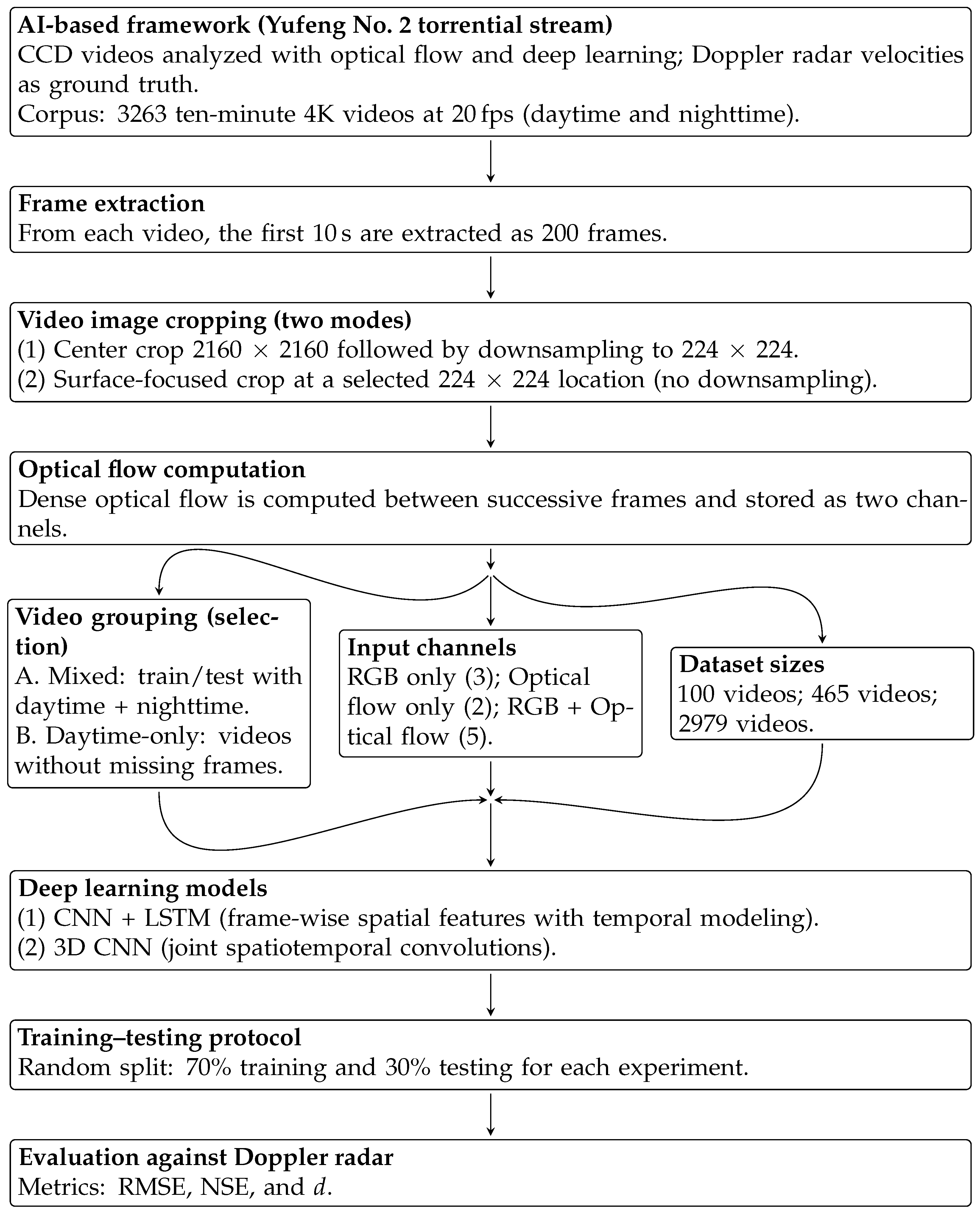
This study develops an end-to-end framework to estimate surface flow velocity from CCD camera videos by integrating dense optical flow computation with deep learning. We analyze a large-scale video corpus collected at the Yufeng No. 2 torrential stream and pair the videos with co-located Doppler radar velocity measurements that serve as reference labels for supervised learning. The materials and methods are organized into the following components: study area and data collection; data preprocessing; model architectures; input configurations; and training, validation, and performance evaluation. An overview of the entire workflow is provided in Figure 1.

Figure 1 summarizes the processing pipeline and experimental design. From each 10 min 4 K video recorded at 20 fps, the first 10 s (200 frames) are extracted. Two cropping protocols are then applied: (i) a center crop of 2160 × 2160 pixels that is downsampled to 224 × 224 and (ii) a surface-focused 224 × 224 patch selected over the water surface without downsampling. Dense optical flow is computed between successive frames and stored as two channels.

The workflow next branches into three parallel experimental factors: (a) video grouping/selection (mixed day+night versus daytime-only videos without missing frames), (b) input channels (RGB-only, optical flow-only, or RGB+flow), and (c) dataset size (100, 465, or 2979 videos). These configurations feed two model families—CNN+LSTM and 3D CNN. For each configuration, models are trained with a 70%/30% train–test split and evaluated against Doppler radar using the Root Mean Square Error (RMSE) [26,27], the Nash–Sutcliffe Efficiency (NSE) [28], and the index of agreement (d) [29]. Detailed descriptions of each block in the flowchart are provided in the subsequent subsections: Study Area and Data Collection, Data Preprocessing, Model Architectures, Input Configurations, and Training, Validation, and Performance Evaluation.

2.1. Study Area and Data Collection

This study was conducted on the Yufeng No. 2 stream (torrent), a small river channel subject to variable flow conditions during rainfall events. Continuous monitoring was implemented using a CCD camera system installed at a fixed location to capture the water surface over time. The monitoring station was positioned to record the stream segment and its interaction with the downstream Yufeng Creek, a trunk river that significantly influences the hydrodynamics of the study area. The broader catchment context is shown in Figure 2, while the site layout and representative camera images are presented in Figure 3. The catchment covers an area of approximately 1.52 km² and is characterized by steep slopes typical of torrential basins in northern Taiwan. The underlying geology comprises alluvium in valley bottoms, with surrounding bedrock formed by the Piling Shale, Shihiti Formation, Shuichangliu Formation (Paling Formation), Talu Shale, and Wenshui Formation. These sedimentary formations are dominated by shale and interbedded rocks that weather rapidly, contributing to slope instability and sediment supply. Soils are generally shallow and coarse-textured, which further promotes rapid runoff. Land cover is overwhelmingly forested, with broadleaf forest accounting for 86.7% (1.32 km²) of the catchment area, followed by bamboo forest at 11.1% (0.17 km²). Small proportions of the area are classified as landslide scars (1.9%), roads (0.16%), orchards (0.11%), and river channels (0.07%). These physical-geographical characteristics, summarized in Figure 2, are important indicators influencing runoff generation, slope stability, and surface flow velocity.

The video dataset consists of 3263 recordings collected between May and June 2025. Each video has a duration of 10 min and a resolution of 4 K (3840 × 2160 pixels). These videos were paired with ground-truth flow velocity measurements obtained from a Doppler radar sensor, which recorded values every 10 min. This pairing provided a reliable reference for model training and validation. Both daytime and nighttime conditions were recorded, although image quality varied significantly between these periods.

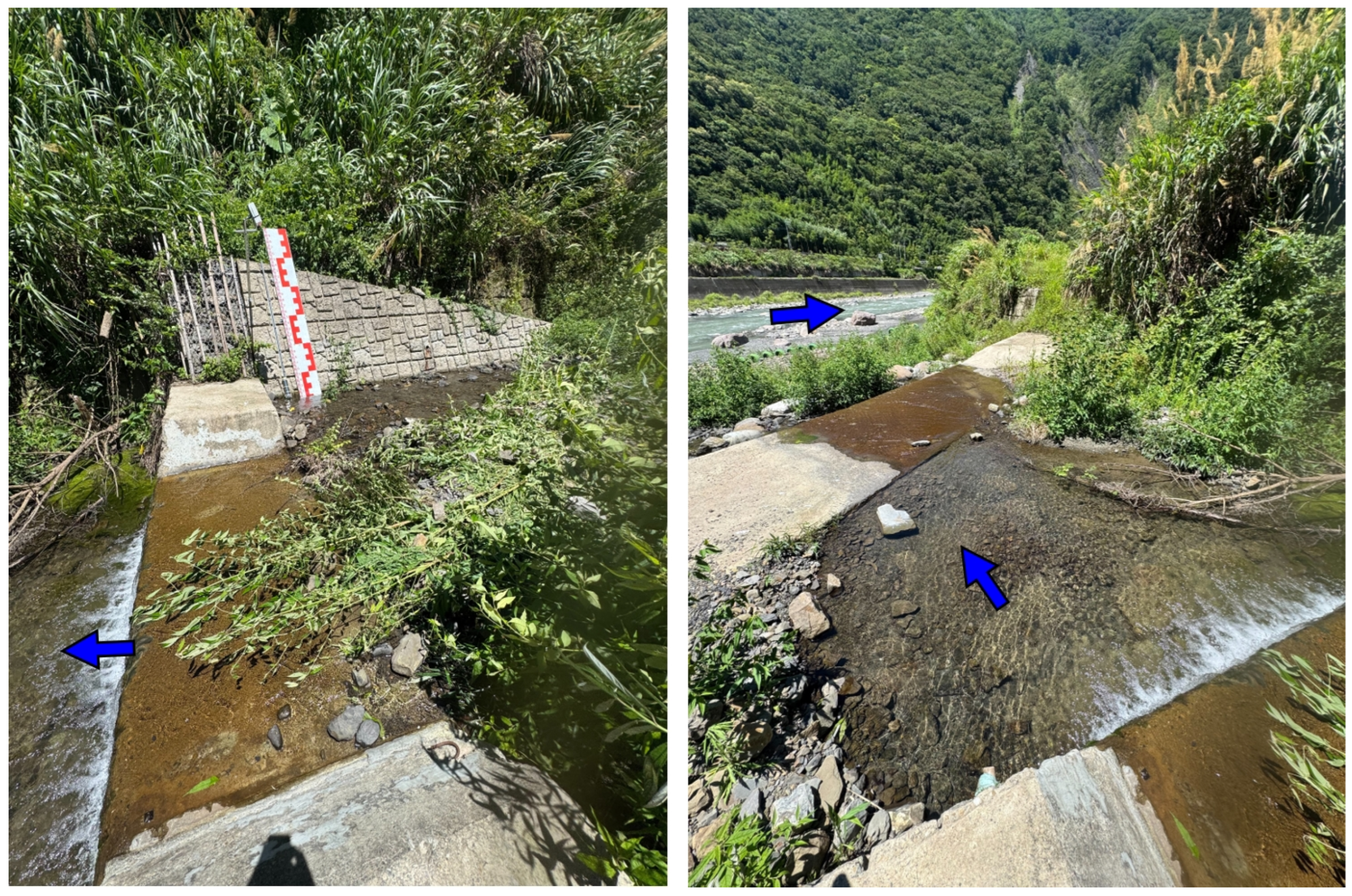
Additional field observations were conducted to document the local channel morphology and hydraulic conditions. Figure 4 shows two photographs taken during the site visit on 23 July 2025. The left image captures the exit of the Yufeng No. 2 stream, while the right image provides a view toward the Yufeng Creek, illustrating the physical connection between the monitored torrent and the main river system.

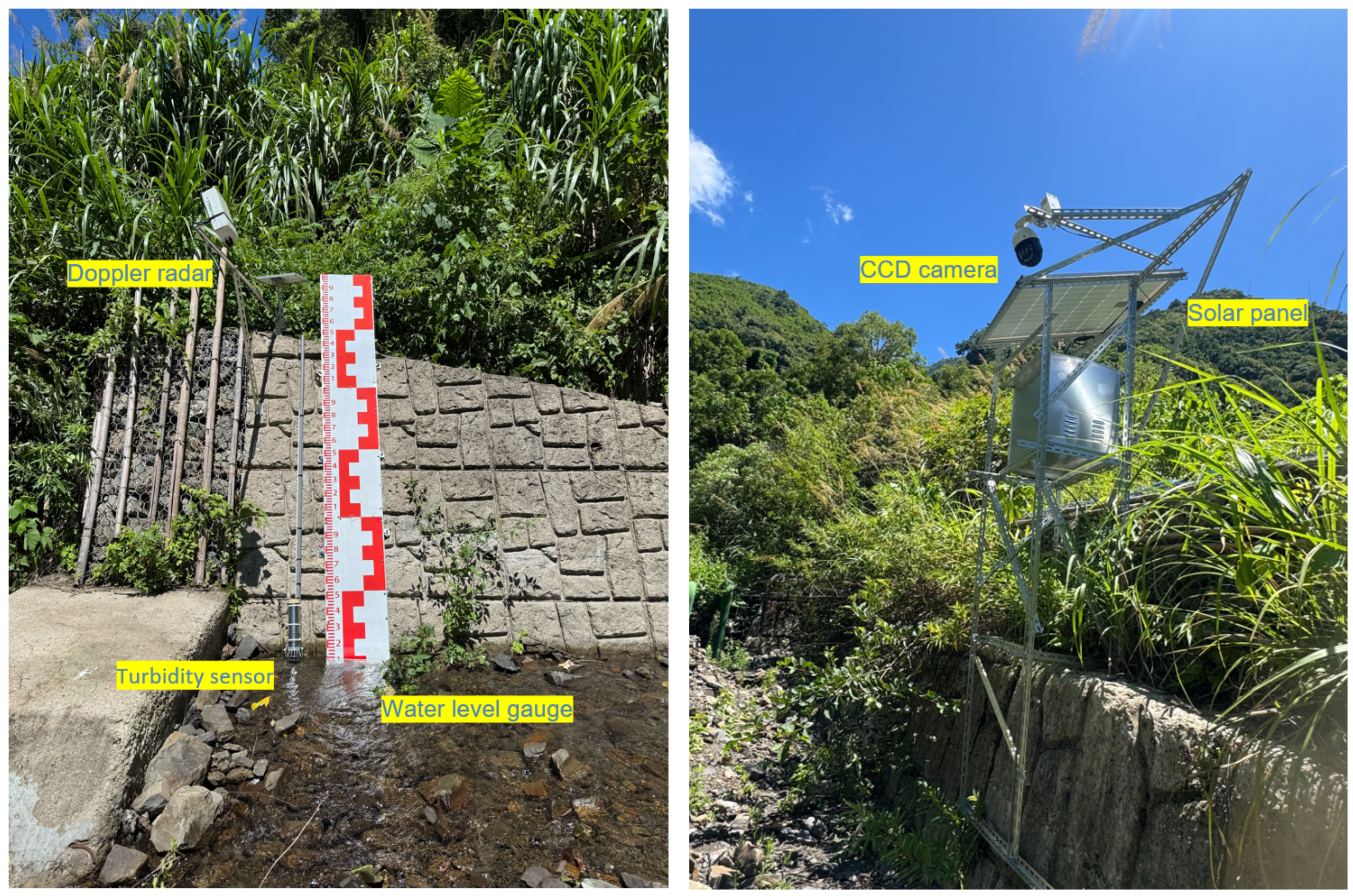
Instrumentation installed at the site included a water level gauge, turbidity sensor, Doppler radar, and a CCD camera powered by a solar panel. Figure 5 illustrates these installations. The left image shows the water level gauge and turbidity measurement device, as well as the position where the Doppler radar was aimed to capture flow velocity. The right image depicts the CCD camera mounted on a steel frame with an integrated solar power system, ensuring continuous operation in remote conditions.

2.2. Data Preprocessing

Preprocessing steps were implemented to ensure the quality and consistency of the dataset. Each 10 min video was sampled to extract a 10 s segment at the beginning, corresponding to 200 consecutive frames at 20 fps. Two different image preparation strategies were applied for model input:

• Full-Scene Downsampling: The central region (as indicated by the orange square in Figure 6) of the original 4 K frame (2160 × 2160 pixels) was extracted and downscaled to 224 × 224 pixels. This approach retained the general scene context while reducing computational cost.
• Focused Cropping: A smaller area of the frame, corresponding to the water surface region (as indicated by the red square in Figure 6), was cropped without downsampling. This method preserved finer spatial details of the flow while excluding background elements such as vegetation and banks that could introduce noise.

Additional preprocessing steps included the following:

• Day/Night Classification: Average brightness thresholds were applied to separate daytime and nighttime videos, as low-light conditions were found to degrade performance.
• Missing Frame Handling: Videos containing missing frames were initially included in the analysis, but their presence was found to degrade model performance. Consequently, in subsequent experiments, such videos were removed, and only continuous sequences of 200 frames were retained.
• Feature Generation: Optical flow was computed using the Farnebäck algorithm [30], producing horizontal and vertical motion components for consecutive frame pairs.

Figure 6 illustrates the two image creation methods used during preprocessing.

2.3. Model Architectures

Two deep learning architectures were developed and evaluated to estimate river flow velocity from video sequences: a CNN+LSTM network and a 3D CNN model. Both architectures were implemented using PyTorch 2.7.1+cu118 and trained to predict a single continuous value representing flow velocity (m/s) from sequences of 200 frames.

• CNN+LSTM: This model combined convolutional neural networks for spatial feature extraction with a recurrent component for temporal modeling. The architecture consisted of the following.
  • Convolutional feature extractor: Each frame was processed by two 2D convolutional layers (Conv2d), with ReLU activations and a 2 × 2 max pooling layer applied after the first convolution. The first layer used 16 filters of size 3 × 3 to extract basic spatial features (e.g., edges and textures), while the second layer increased the depth to 32 feature maps, capturing more complex flow-related structures.
  • Global pooling: An Adaptive Average Pooling layer reduced each feature map to a 1 × 1 representation, resulting in a 32-dimensional feature vector per frame.
  • Sequence modeling: The extracted feature vectors from 200 frames formed an input sequence of size [B, T, 32], where B is batch size and $T=200$. This sequence was processed by a single LSTM layer with 64 hidden units to learn temporal dependencies across frames.
  • Fully connected layer: The final hidden state of the LSTM was passed through a linear layer (64 → 1) to output the predicted flow velocity.

The CNN+LSTM design allowed the network to first focus on extracting per-frame spatial characteristics and then model their evolution over time.

• 3D CNN: In contrast to the sequential approach, the 3D CNN jointly captured spatial and temporal patterns using three-dimensional convolution kernels. The architecture included the following.
  • Spatiotemporal convolutions: Two Conv3d layers with ReLU activations processed the input tensor of size [B, C, T, H, W], where C represents channels (RGB or optical flow components), T is the temporal dimension (200 frames), and H and W are frame height and width. The 3D kernels (e.g., 3 × 3 × 3) extracted local motion and texture features across both space and time.
  • Pooling layers: MaxPool3d operations were used after each convolutional layer to reduce spatial and temporal dimensions while preserving essential patterns.
  • Global average pooling: An AdaptiveAvgPool3d layer compressed the feature maps into a fixed-length 32-dimensional vector summarizing the entire video sequence.
  • Output layer: The pooled feature vector was passed through a fully connected layer to predict a single velocity value.

This architecture leveraged end-to-end learning of spatiotemporal features without requiring explicit sequence modeling, making it computationally efficient for short video segments.

To clarify when each architecture is preferable in this application,

Table 1. Concise comparison of the two deep learning architectures used in this study.

Aspect	CNN+LSTM	3D CNN
Modeling strategy	2D CNN per frame with an LSTM to model the 200-frame temporal sequence.	3D convolutions learn joint space–time features directly from the video volume.
Strengths	Leverages longer temporal context; tolerant of occasional dropped/blurred frames.	Captures motion patterns end to end; simple pipeline (no explicit sequence module).
Limitations	May miss very localized fast motions unless the CNN is deeper.	More sensitive to frame-rate gaps/exposure changes if preprocessing is weak.
Works best when / data considerations	Daytime scenes with moderate texture; when longer context aids disambiguation.	Short, clean clips with stable camera/exposure and strong motion cues.
Compute and runtime (this study)	Efficient on a desktop PC with a recent NVIDIA GPU; completes in minutes for small subsets. Around ∼3000 videos, total time can reach tens of minutes.	Also efficient and typically faster than CNN+LSTM under the same settings; minutes for small subsets; tens of minutes at ∼3000 videos.

contrasts the CNN+LSTM and 3D CNN along their principal advantages and limitations, applicability, data quality requirements, and expected differences in accuracy and computational efficiency under this study’s setting (200-frame clips at 224 × 224 with RGB and/or optical flow channels).

Both models were trained using the Adam optimizer (learning rate = 0.001) with mean squared error (MSE) as the loss function. A batch size of 4 was used, and training was conducted for 10 epochs. The best-performing model based on validation loss was saved for subsequent evaluation.

2.4. Input Configurations

Three input configurations were tested to evaluate the effect of different feature representations on model performance. Each configuration used sequences of 200 consecutive frames extracted from a 10 s segment of video. The input tensors followed the general shape [B, C, T, H, W], where

• B: Batch size;
• C: Number of channels (depends on feature type);
• T: Temporal dimension (number of frames = 200);
• H, W: Frame height and width (224 × 224 pixels after preprocessing).

The three configurations were as follows:

• RGB frames only: Each frame was represented by three color channels (red, green, and blue).

  $$\mathrm{Input}\mathrm{shape}:[B, 3, 200, 224, 224]$$
  This configuration preserved color information, which could provide contextual cues but did not explicitly encode motion.
• Optical flow fields: Motion features were computed using the Farnebäck algorithm [30] for each pair of consecutive frames. Two channels were generated per frame: horizontal displacement (u) and vertical displacement (v). To ensure a consistent sequence length of 200 frames, an additional all-black frame was appended at the end of each sequence.

  $$\mathrm{Input}\mathrm{shape}:[B, 2, 200, 224, 224]$$
  This representation focused entirely on capturing motion dynamics without color information.
• Combined RGB and optical flow (feature-level fusion): RGB frames and optical flow channels were concatenated along the channel dimension, forming a five-channel input (3 RGB channels + 2 optical flow channels).

  $$\mathrm{Input}\mathrm{shape}:[B, 5, 200, 224, 224]$$
  This approach aimed to integrate spatial context and motion information within a single input tensor.

2.5. Training, Validation, and Performance Evaluation

All analyses were implemented in Python (version 3.11.13) within the Anaconda environment. Deep learning models were developed and trained using the PyTorch framework, with NumPy employed for numerical computations, Pandas for data handling, and Matplotlib for visualization. Model evaluation metrics (RMSE, NSE, and d) were implemented directly in Python to ensure reproducibility.

The dataset was randomly divided into 70% for training and 30% for testing to ensure unbiased evaluation of model performance. Training was conducted for multiple epochs with no early stopping based on validation loss to prevent overfitting.

To examine the influence of dataset size on model performance, experiments were performed using progressively larger subsets of the available videos, including 100, 465, and 2979 samples. Additionally, separate experiments were conducted on daytime-only datasets to assess the effect of illumination and image quality, as nighttime videos were found to contain frequent frame losses and reduced clarity.

An overview of the workflow, including the preparation of training and testing subsets, is illustrated in Figure 1.

Model performance was evaluated using three indicators:

• RMSE [26,27]: Quantifies the average magnitude of prediction errors, with lower values indicating better accuracy.
• NSE [28]: Evaluates predictive performance relative to the observed mean. Values close to 1 indicate high predictive skill, while values less than 0 suggest performance worse than the mean model.
• d-statistic [29]: Measures the degree of agreement between observed and predicted values, with values closer to 1 representing higher concordance.

The explicit formulations of these three evaluation metrics are provided below:

$$\mathrm{RMSE}=\sqrt{{\displaystyle \frac{1}{N}}\sum _{i=1}^N{(v_i-{\widehat{v}}_i)}^2}$$

(1)

$$\mathrm{NSE}=1-{\displaystyle \frac{{\sum }_{i=1}^N{(v_i-{\widehat{v}}_i)}^2}{{\sum }_{i=1}^N{(v_i-\overline{v})}^2}}$$

(2)

$$d=1-{\displaystyle \frac{{\sum }_{i=1}^N{(v_i-{\widehat{v}}_i)}^2}{{\sum }_{i=1}^N{\left(\left|{\widehat{v}}_i-\overline{v}\right|+\left|v_i-\overline{v}\right|\right)}^2}}$$

(3)

where

$$\begin{array}{cc}\hfill v_i& =\mathrm{Observed}\mathrm{water}\mathrm{flow}\mathrm{velocity}\mathrm{at}\mathrm{instance}i;\hfill \\ \hfill {\widehat{v}}_i& =\mathrm{Predicted}\mathrm{water}\mathrm{flow}\mathrm{velocity}\mathrm{at}\mathrm{instance}i;\hfill \\ \hfill \overline{v}& =\mathrm{Mean}\mathrm{of}\mathrm{observed}\mathrm{water}\mathrm{flow}\mathrm{velocities};\hfill \\ \hfill N& =\mathrm{Total}\mathrm{number}\mathrm{of}\mathrm{observations}.\hfill \end{array}$$

3. Results

A series of experiments were conducted to evaluate the performance of the proposed framework under different model architectures and input configurations. The main focus was to assess how the choice of features (RGB, optical flow, and RGB+flow) and the network architecture (CNN+LSTM vs. 3D CNN) affected prediction accuracy. Additionally, the impact of training dataset size and video quality on model performance was analyzed.

3.1. Effect of Image Cropping on Model Performance

The first comparison evaluated the impact of different image preprocessing strategies on model performance:

• Full-scene downsampling: The central region of the original 4K frame was downscaled to 224 × 224 pixels.
• Cropped water surface: The water surface area was cropped without downsampling, preserving more detailed flow features.

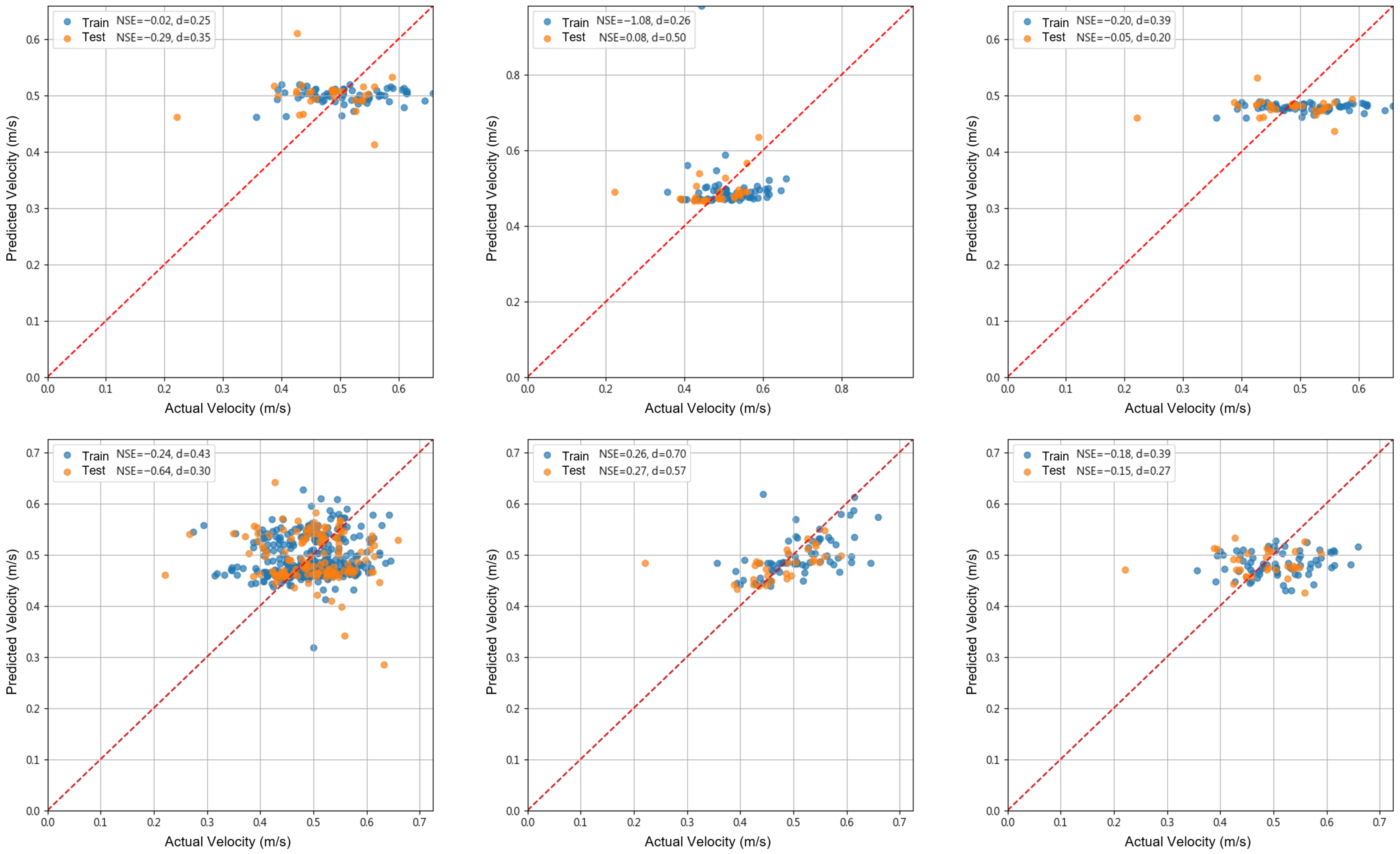
Experiments were conducted using 100 video samples under three input configurations: (i) RGB frames only, (ii) optical flow fields, and (iii) combined RGB and optical flow (feature-level fusion). Figure 7 presents a visual summary of the results for these configurations, organized into a 2 × 3 layout: the first row corresponds to full-scene images and the second row corresponds to cropped water surface images. The columns represent RGB-only, optical flow-only, and combined RGB+flow inputs, respectively. Each plot displays the predicted versus observed flow velocities for the training and testing sets, along with corresponding NSE and d-statistic values.

The results indicate that cropping the water surface region consistently yielded better performance compared to using full-scene downsampled images. This improvement is attributed to the elimination of irrelevant background elements such as vegetation and channel banks, which can introduce noise into feature extraction. Across all experiments, optical flow inputs achieved the highest accuracy, while RGB-only inputs performed the worst. The combined RGB and optical flow configuration produced intermediate results, generally better than RGB alone but not surpassing optical flow by itself. These findings suggest that focused cropping enhances the discriminative capacity of motion-based features and that adding RGB information does not necessarily improve performance when motion cues dominate the prediction task.

3.2. Effect of Training Dataset Size

The impact of increasing the training dataset size on model performance was examined using three different subsets: 100, 465, and 2979 videos. The objective was to determine whether larger datasets could significantly improve prediction accuracy. All experiments in this comparison used cropped water surface images under three input configurations: (i) RGB frames only, (ii) optical flow fields, and (iii) combined RGB and optical flow (feature-level fusion).

Figure 8 illustrates the results for the two largest subsets (465 and 2979 videos) arranged in a 2 × 3 layout. The first row corresponds to the 465-video set and the second row corresponds to the 2979-video set. Columns represent RGB-only, optical flow-only, and combined RGB+flow inputs, respectively. For reference, the case using 100 videos is presented earlier in Figure 7. Each plot shows predicted versus observed flow velocities for both training and testing sets, along with the corresponding NSE and d-statistic values.

The results confirm that increasing the number of training videos from 100 to 465 and then to 2979 yielded minimal performance improvement across all input configurations. NSE values remained largely unchanged, indicating that the model’s predictive capability was not substantially enhanced by additional data. These findings suggest that the primary limitation lies in the quality of input data rather than dataset size. Simply enlarging the dataset without ensuring high-quality inputs does not guarantee better accuracy. Future improvements should therefore prioritize collecting high-resolution videos under consistent lighting conditions and minimizing frame loss, as these factors strongly influence model performance.

3.3. Effect of Video Quality: Daytime vs. Nighttime Analysis

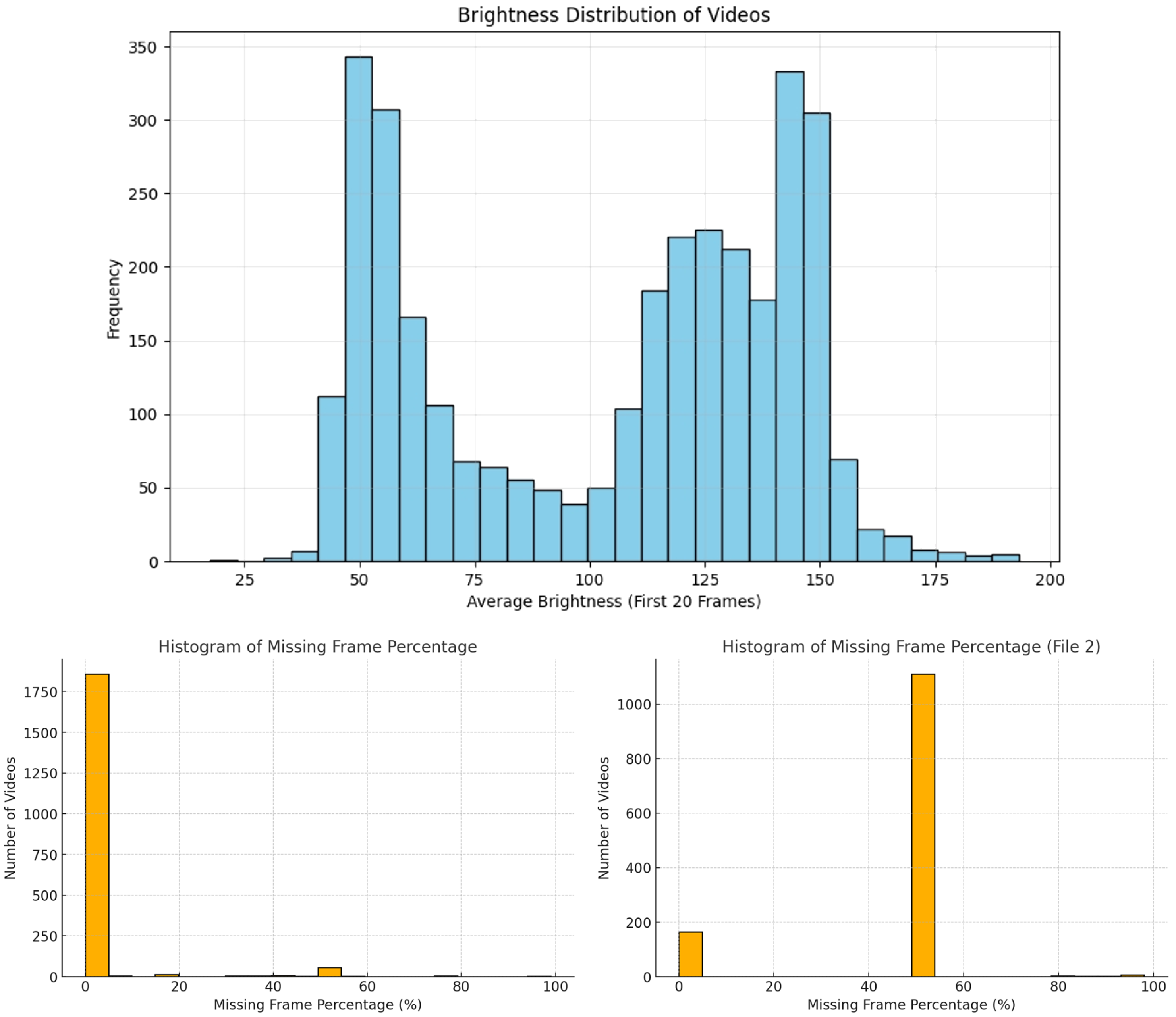
All previous experiments employed a randomly mixed dataset of daytime and nighttime videos, which resulted in unsatisfactory performance, as indicated by low NSE and d values. To identify the underlying causes, video quality was evaluated based on two key factors: brightness distribution and the proportion of missing frames.

Figure 9 presents three plots summarizing these analyses. The first plot shows the brightness distribution of all videos, which exhibits a clear bimodal pattern. Videos with higher brightness values correspond to daytime conditions, whereas those with lower brightness represent nighttime recordings. This distinction was used to classify videos into daytime and nighttime subsets.

The second and third plots illustrate the distribution of missing frame percentages for daytime and nighttime videos, respectively. Daytime videos generally exhibited very low frame loss, with most videos having nearly complete frame sequences. In contrast, nighttime videos suffered severe frame loss, with the majority of videos missing 40–60% of frames. This loss is primarily attributed to low-light conditions, which also degrade the quality of optical flow estimation.

To further validate the effect of video quality, the models were retrained using only daytime videos with no missing frames (a total of 1712 videos). The same model architectures and hyperparameters as in previous experiments were used to ensure a consistent comparison. Figure 10 presents the results for RGB-only, optical flow-only, and combined RGB+flow inputs.

The results demonstrate a critical insight: the poor performance observed in previous experiments was not due to deficiencies in the model architecture but rather to the quality of the input data. When trained with high-quality videos, the optical flow-based model achieved an NSE value above 0.5 (0.53), a threshold often considered acceptable for hydrological predictions. This finding underscores the importance of rigorous data quality control in developing reliable AI-based flow estimation systems. Future work should focus on addressing the challenges of nighttime video quality through image enhancement techniques or improved hardware, rather than solely relying on more complex model designs.

3.4. Influence of Input Configurations

Three input configurations were evaluated across all experiments: (i) RGB frames only, (ii) optical flow fields, and (iii) combined RGB with optical flow (feature-level fusion). The results from Figure 7, Figure 8 and Figure 10 consistently demonstrate clear performance differences among these configurations.

Models trained exclusively on RGB inputs exhibited the weakest predictive capability, often producing outputs close to the mean flow velocity regardless of actual variation. This behavior suggests that color information alone provides insufficient dynamic cues for representing surface flow patterns, leading to poor generalization and low NSE values.

In contrast, optical flow-based inputs consistently outperformed RGB-only inputs across all scenarios, including variations in image preprocessing (full-scene vs. cropped), dataset size (100, 465, and 2979 videos), and video quality (mixed day/night vs. daytime-only). Optical flow directly captures motion information between consecutive frames, which is essential for inferring flow velocity and explains its superiority as a feature representation.

Combining RGB and optical flow channels through feature-level fusion consistently resulted in lower performance compared to using optical flow alone. Across all cases (Figure 7, Figure 8 and Figure 10), fusion degraded accuracy, as reflected by reduced NSE values. This finding underscores a critical insight: incorporating additional feature channels does not necessarily enhance model performance and may instead introduce noise or redundant information that hinders learning. For this application, motion-based features derived from optical flow are the dominant contributors to predictive accuracy, whereas static color features provide limited value.

These findings underscore the importance of carefully selecting informative features rather than assuming that more input data will inherently enhance model performance.

3.5. Comparison of Model Architectures

The CNN+LSTM and 3D CNN architectures exhibited different strategies for modeling spatial and temporal information. CNN+LSTM extracted frame-level features sequentially using convolutional layers and aggregated them through an LSTM layer to capture temporal dependencies. In contrast, the 3D CNN processed the entire video segment as a spatiotemporal block, allowing simultaneous learning of spatial and temporal patterns through 3D convolutional kernels.

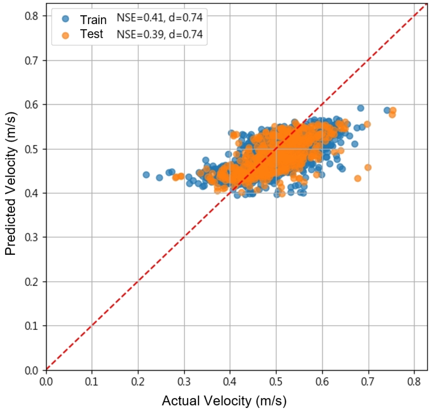
Previous figures (i.e., Figure 10, center panel) demonstrated that the 3D CNN, when combined with optical flow inputs, achieved an NSE exceeding 0.5 (0.53), which meets the threshold commonly regarded as acceptable for hydrological prediction tasks. To compare architectures under the same conditions, Figure 11 presents the results obtained using the CNN+LSTM architecture with optical flow inputs and the same set of 1712 high-quality daytime videos.

The comparison reveals that 3D CNN outperformed CNN+LSTM under identical experimental conditions. While CNN+LSTM achieved moderate agreement between predicted and observed velocities, its NSE value remained below the threshold of 0.5 (0.39), whereas the 3D CNN surpassed this level (Figure 10). This performance gap can be attributed to the inherent differences in design: LSTM layers are primarily suited for time-series forecasting, where predicting the next observation in the sequence is critical. In this application, the task is to estimate an aggregated property (mean flow velocity) for an entire video segment rather than forecast the next frame. Consequently, the 3D CNN’s ability to jointly model spatial and temporal correlations without relying on sequential recurrence provides a more effective representation of flow dynamics.

3.6. Performance Metrics and Trade-Offs

Performance was quantified using RMSE, NSE, and the d statistic. Models using optical flow and 3D CNN achieved NSE values greater than 0.5, meeting the minimum threshold for acceptable predictive performance. In contrast, CNN+LSTM models generally produced lower NSE values. Notably, NSE and d did not always align: certain models achieved higher d scores despite poor NSE. This discrepancy underscores that NSE, which captures variance and extreme values, is a more critical metric for flood risk applications, where underestimating high-flow conditions can lead to significant hazards. Nevertheless, NSE alone is not always sufficient, and in other contexts it may be misleading; thus, it is best interpreted in conjunction with RMSE and other complementary metrics.

3.7. Key Observations

The experimental results support several important findings:

• Optical flow combined with 3D CNN provided the most accurate and robust predictions.
• RGB features and RGB+flow fusion offered no improvement over optical flow alone.
• Increasing training data beyond approximately 100 videos did not enhance accuracy.
• High-quality input data is essential; poor nighttime video quality significantly reduced performance.
• NSE is a more relevant performance indicator than d for operational safety; however, it should be interpreted alongside RMSE and other metrics for a balanced assessment.

3.8. Implications for Practical Deployment

These findings indicate that AI-driven flow monitoring systems can achieve reliable performance using optical flow-based deep learning models, provided that video quality is controlled and model design is optimized. The limited benefit of adding RGB features or enlarging the dataset suggests that future efforts should prioritize collecting high-quality videos, enhancing feature quality (e.g., better optical flow algorithms or adaptive cropping), and expanding the velocity range in training data. Real-time deployment is feasible due to the relatively modest computational requirements of the 3D CNN framework once trained.

3.9. Limitations and Future Directions

Although the proposed framework demonstrates promising results, several limitations should be acknowledged. First, the available dataset is concentrated in May–June and thus reflects mid–low-discharge conditions, with high-flow episodes (e.g., typhoon or flood peaks) underrepresented; accordingly, the range of flow velocities in the dataset is relatively narrow, which may restrict the generalization of the trained models to extreme flow conditions. Augmenting the corpus with videos acquired during typhoons and post-heavy-rainfall periods, so that low-, medium-, and high-flow regimes are all covered, is necessary for improving robustness.

Second, nighttime videos exhibited severe frame loss and poor illumination, significantly reducing the reliability of optical flow estimation. While filtering out these low-quality videos improved performance, this approach limits operational flexibility. Future work should explore techniques for low-light image enhancement or the use of cameras with better night-vision capability to ensure consistent data quality.

Third, the current study focuses on a single site. Subsequent work should extend to settings with different river types and geomorphic conditions and systematically examine differences in camera deployment (e.g., mounting height, view angle, and lens), acquisition parameters (e.g., frame rate and exposure), and resultant model performance. Such experiments will enable a more rigorous assessment of model generalization and practical transferability.

Fourth, while the 3D CNN architecture outperformed CNN+LSTM, this study evaluated only two model types. Exploring more advanced architectures, such as attention-based spatiotemporal networks or transformers, could further improve performance. In addition, the present study did not include explicit interpretability analyses (e.g., attribution of important spatial regions or temporal frames). Although some evidence of spatial focus was obtained through the cropping experiments (Section 3.1, Figure 6), more detailed approaches such as saliency mapping could be explored in future work.

Fifth, the framework was developed as an image-based regression system, with Doppler radar serving as the ground truth rather than as a time-series model of velocity dynamics. Future studies could investigate incorporating temporal dependencies across successive video segments to evaluate the ability of such models to capture variability in flow magnitude over time.

Finally, the current framework was tested in an offline setting. Future efforts should focus on optimizing computational efficiency and deploying the system for real-time monitoring, which is critical for flood early warning systems and disaster management applications.

4. Discussion

The present study demonstrated that integrating dense optical flow with deep learning architectures can provide accurate estimates of river surface velocity from fixed CCD camera videos. By comparing CNN+LSTM and 3D CNN models, we found that the 3D CNN with optical flow-only inputs consistently delivered superior predictive performance. This outcome underscores the importance of motion-based features for hydrological monitoring, as optical flow directly encodes pixel-wise displacement, whereas RGB imagery may introduce redundant appearance information even when limited to the water surface.

The experiments also highlighted that video quality and preprocessing strongly influence model accuracy. The comparison between full-scene downsampling (orange square) and cropped water surface input (red square) (Figure 6) confirmed that focusing solely on the water surface reduces noise and improves predictive skill. Similarly, excluding low-quality nighttime videos enhanced reliability, reinforcing the need for careful data screening or future image enhancement approaches. These results emphasize that video preprocessing decisions are not merely technical adjustments but fundamentally affect model learning.

While the current analysis produced encouraging results, interpretability remains a significant challenge. Deep neural networks are often criticized as “black boxes,” and hydrological applications require trust in their predictions. The red square water surface cropping experiment provided some insight into the model’s spatial focus; however, more advanced interpretability tools, such as saliency maps or gradient-based visualizations, could further reveal how specific spatial patterns or temporal sequences contribute to velocity estimation. Future work should explore these methods to complement the quantitative evaluation.

Another methodological aspect relates to temporal representation. The models in this study were trained as image-based regression systems, predicting velocity from video data without explicitly modeling temporal correlations across successive sequences. While this design aligns with our objective of mapping visual motion to Doppler radar measurements, future research may investigate video-to-video learning frameworks to capture longer-term dynamics in flow variability.

An important practical consideration is the performance of the monitoring system under extreme hydrological events. The dataset analyzed here (3263 recordings) was collected between May and June 2025, a period without typhoons affecting the study area or high-intensity rainfall events. The model is therefore reliable only within the observed velocity ranges. Future collection during typhoons and storm events will be essential for retraining and calibration. In addition, severe events may pose risks to the field equipment. Although the camera system was securely installed, extreme flows with coarse sediments, stones, or woody debris could damage the devices. Addressing such risks will be critical for long-term operational deployment and for linking this framework with flash flood and soil erosion studies.

A comparison with related work further highlights the characteristics of our dataset. Cao et al. [25] employed 52 videos spanning a wide velocity range of approximately 0–6.0 m/s, although most of their observations were concentrated below 1.5 m/s. By contrast, our dataset comprises 3263 recordings—substantially larger in size but with a narrower velocity distribution of about 0.2–0.8 m/s (Figure 10)—reflecting the fact that no typhoon or high-intensity rainfall events affected the study area during the May–June 2025 collection period. Their study reported a surface velocity estimation accuracy of 92.03% and an average relative error of 11.61%. While the reported accuracy appears higher than ours, their relative error is greater. Moreover, given that their analysis was based on only 52 videos, the overall scale of our dataset is much larger, although the minimum data requirement for establishing a baseline evaluation appears comparable to theirs.

Overall, the findings confirm that combining optical flow with deep learning is a promising approach for non-intrusive river velocity monitoring. The results also point to several areas for further research, including the pursuit of interpretability methods, the incorporation of explicit temporal models, and data collection under a wider range of hydrological conditions. These directions will be important for enhancing model robustness and ensuring practical applicability in flood forecasting and water resource management.

The specific methodological and data-related constraints of this study, as well as directions for future work, are further detailed in Section 3.9.

5. Conclusions

This study introduced an AI-based framework for estimating river flow velocity from CCD camera videos, combining dense optical flow features with deep learning architectures. Two model types were examined: CNN+LSTM and 3D CNN. Among the tested configurations, optical flow paired with a 3D CNN consistently achieved the best predictive performance, with NSE values exceeding 0.5 under high-quality video conditions. These results demonstrate the feasibility of using video-based computer vision methods for non-intrusive hydrological monitoring.

Several key insights emerged. First, data quality proved to be a dominant factor: videos without missing frames and with adequate illumination yielded substantially higher accuracy, whereas low-quality nighttime footage degraded performance. Second, adding RGB channels or increasing the dataset size without accounting for data characteristics did not necessarily improve predictive skill. These findings highlight the importance of targeted feature selection and careful preprocessing in the development of vision-based hydrological tools.

The practical implications of this framework are significant. With further refinement, optical flow-based deep learning models could support continuous river monitoring, contribute to flash flood early warning systems, and provide valuable input for soil erosion and sediment transport studies. Future work should focus on extending the dataset to include extreme hydrological events, improving interpretability of model predictions, and assessing transferability across diverse riverine environments. Together, these efforts will move toward operational, real-time applications of AI-driven river flow monitoring.